Research on Transformer Voiceprint Anomaly Detection Based on Data-Driven

Abstract

Condition diagnosis of power transformers using acoustic signals is a nonstop, contactless method of equipment maintenance that can diagnose the transformer’s type of abnormal condition. To heighten the accuracy and efficiency of the abnormal method of diagnosing abnormalities by sound, a method for abnormal diagnosis of power transformers based on the Attention-CNN-LSTM hybrid model is proposed. This collects the sound signals emitted by the real power transformer in the normal state, overload, and the discharge condition. It preprocesses the sound signals to obtain the MFCC characteristics of the sound signals. It is then grouped into a set of sound feature vectors by the first- and second-order differences, and enters the Attention-CNN-LSTM hybrid model for training. The training results show that the Attention-CNN-LSTM hybrid model can be used for the status sound detection of power transformers, and the recognition of the three states can achieve an accuracy rate of more than 99%.

1. Introduction

The power transformer is one of the most important pieces of equipment in the power system. The state in which it operates has a direct impact on the power supply and the safety of the power system. With the increase in user electricity consumption, more and more transformers are invested in the power grid, so transformer monitoring and fault-detection technology play a vital role in the power grid’s fault-prevention ability and safe and steady operation.

The failure of power transformers is mainly based on insulation failures, and some noninsulating primary faults can be converted into insulation faults. A variety of factors cause the factors that lead to insulation deterioration of transformers [1,2]. Currently, the primary methods for transformer abnormality and fault diagnosis are oil chromatography diagnosis, vibration diagnosis, infrared thermal imaging diagnosis, acoustic diagnosis, and spectral diagnosis [3,4,5,6,7,8,9,10,11]. Among these diagnostic methods, acoustic diagnosis has the advantages of easy assembly, fast diagnosis, and no direct contact with equipment compared with other diagnostic methods. Usually, sound methods for abnormalities and fault diagnosis are judged mainly by experienced people through the human ear. However, this method has a large human impact and is only suitable for more obvious failure occurrences.

Deep learning machine learning models based on neural networks have emerged as the prevalent trend as machine learning gains popularity. The use of deep learning to judge faults has also been applied to many fields and has gained excellent results [12,13,14,15]. In the research of transformer voiceprint fault detection, the literature [16] proposes a model based on Mel time spectrum-convolutional neural network transformer core voiceprint recognition, through the vibration signal and sound data of the iron core under different operating states to achieve the identification of three voltage conditions. Although the recognition accuracy of this method for three working conditions has reached 99%, it is necessary to install vibration sensors and sound sensors, which are more complex in practical applications, and the installation position has a more significant impact on experimental results. The literature [17] proposes a backpropagation (BP) neural network diagnostic model based on transformer vibration and noise, by acquiring transformer vibration and noise signals, obtaining eigenvalues after fast Fourier transformation. Entering them into the BP neural network for fault diagnosis, this method is more accurate for obvious mechanical fault identification, but the recognition accuracy for transformer discharge, overload, and other abnormal phenomena is low. The literature [18] proposes a transformer voiceprint recognition model based on improved Mel-frequency cepstral coefficients (MFCC) and vector quantization (VQ) algorithms, first used for computational recognition by principal component analysis and VQ algorithm, and the recognition accuracy rate reaches 93%. Although this method retains most of the MFCC characteristics, the difference between the sounds of different operating conditions of the transformer may exist in the discarded MFCC, so this method is less accurate in identifying abnormalities when the transformer’s sound is not obvious.

As to the above problems, a hybrid transformer abnormal voiceprint recognition model that uses MFCC combined with convolutional neural networks (CNNs) and long short-term memory (LSTM) is proposed. It collects the normal operation of the substation 10-kV oil-immersed transformer and the sound of abnormal (overload and discharge as an example). These three states are samples collected under load on the transformer, and the two abnormal states of discharge and overload are samples recorded by the substation during the previous operation of the transformer; an abnormal discharge state refers to a partial discharge. MFCC is used to feature the collected sound, and after that the extracted sound features are introduced to the CNN-LSTM hybrid model, and the attention mechanism is introduced to identify the three working conditions of the transformer accurately.

2. Acquisition and Analysis of Transformer Sound Signals

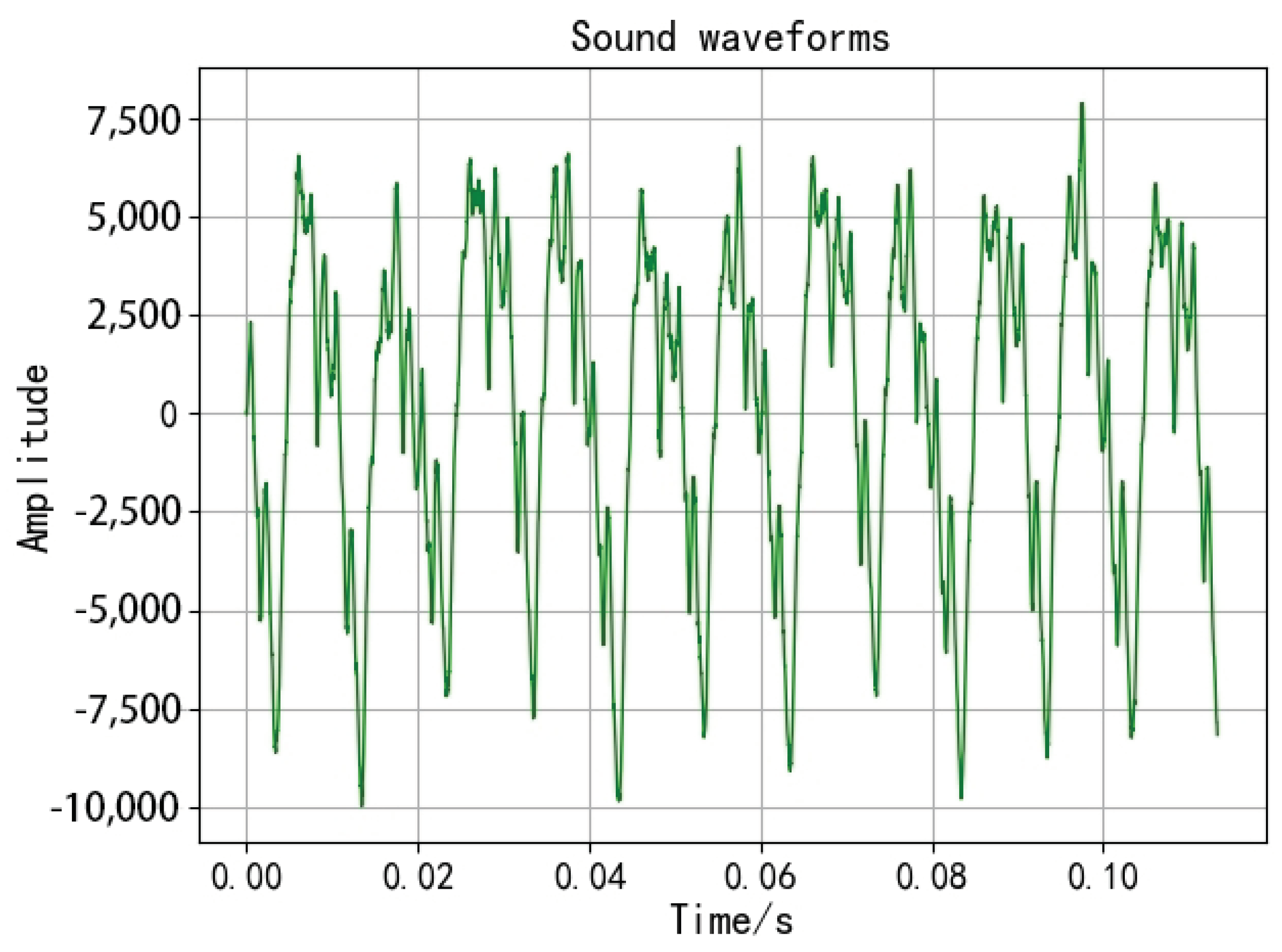
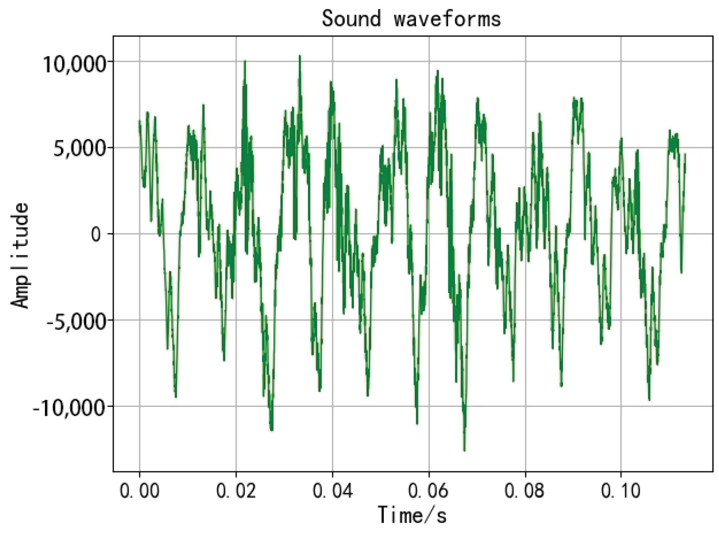
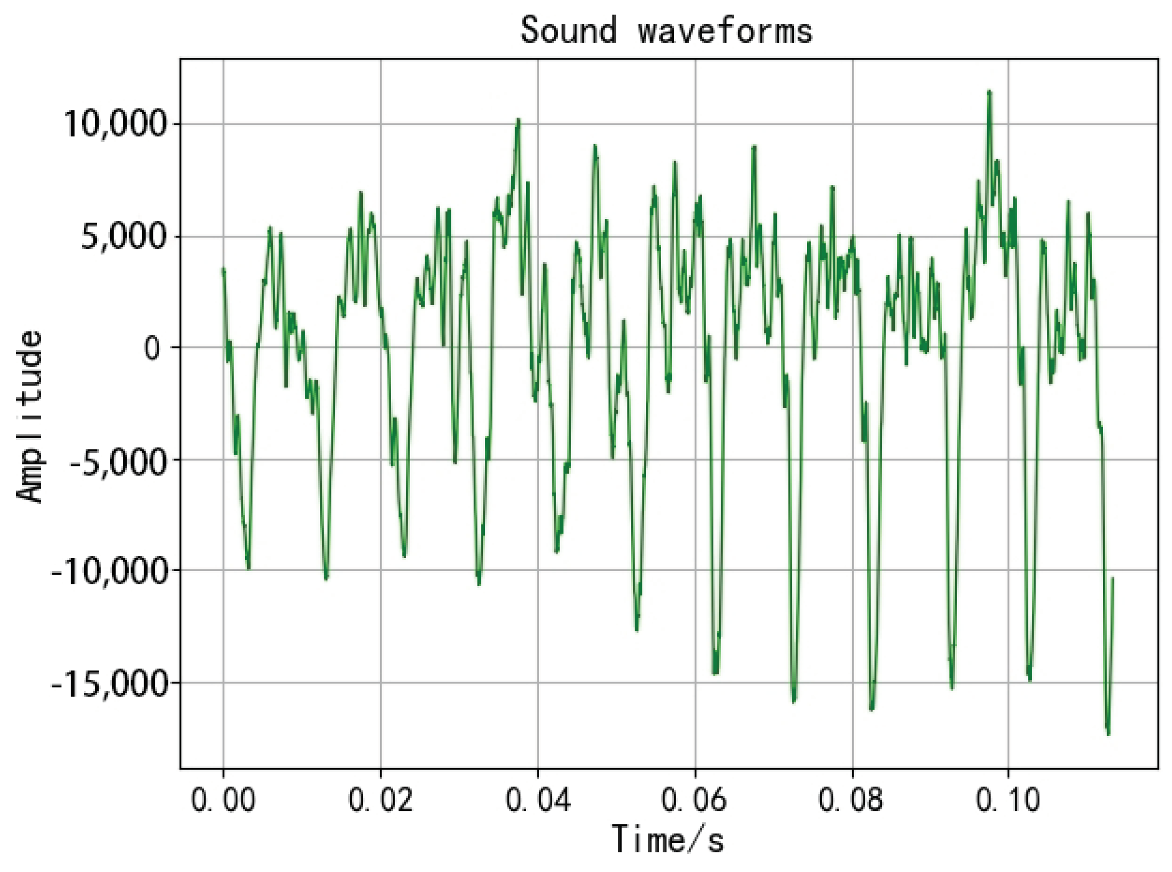
2.1. Time Domain Analysis

Transformer vibrations through the windings, core, insulating oil, and other accessories, move outward in the form of sound through the transformer tank. The sound contains a wealth of equipment status information. In terms of the sound acquisition, a computer is used to connect the DAC sound card and microphone, a microphone is fixed close to the core of the transformer, and the cycle acquisition is set with 10 s as a sample. The sensor for the microphone is an electret condenser with a sensitivity of −30 dB +/−3 dB and a signal-to-noise ratio of 74 dB SPL. The sound card adopts a no-noise reduction card, the acquisition frequency band covers 0–22,000 Hz, the sampling frequency is 44,100 Hz, and the sampling channel is mono. Figure 1, Figure 2 and Figure 3 show the time domain waveform diagram of the transformer under normal, overload, and discharge conditions. The transformer operates in a normal state, and the AC will generate alternating magnetic flux through the winding. This magnetic flux has a periodicity that will cause periodic vibration of the iron core [19]. This sound is regular, as shown in the time domain waveform diagram in Figure 1. If the transformer is discharged, the sound of the engine operation will be mixed with the sound of discharge, and the regularity of the sound is not obvious in the normal state, as shown in Figure 2. In the event of an overload, the engine hums louder than during normal operation [20] as shown in Figure 3.

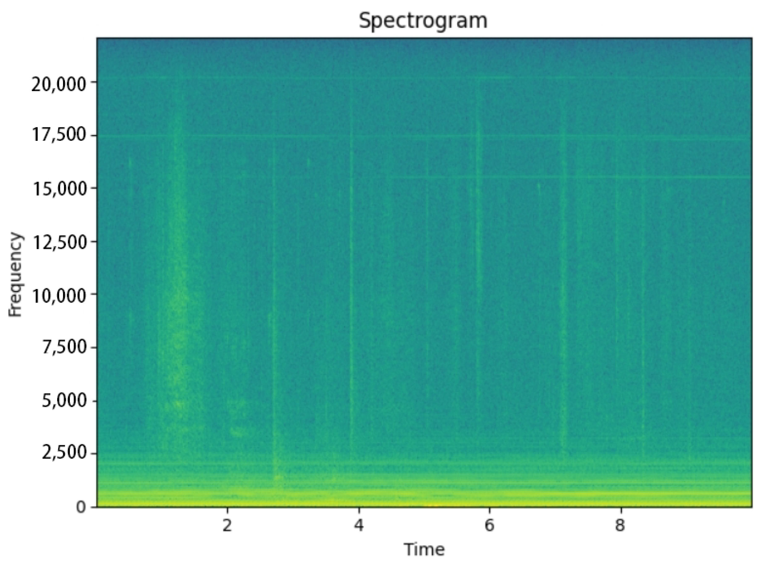
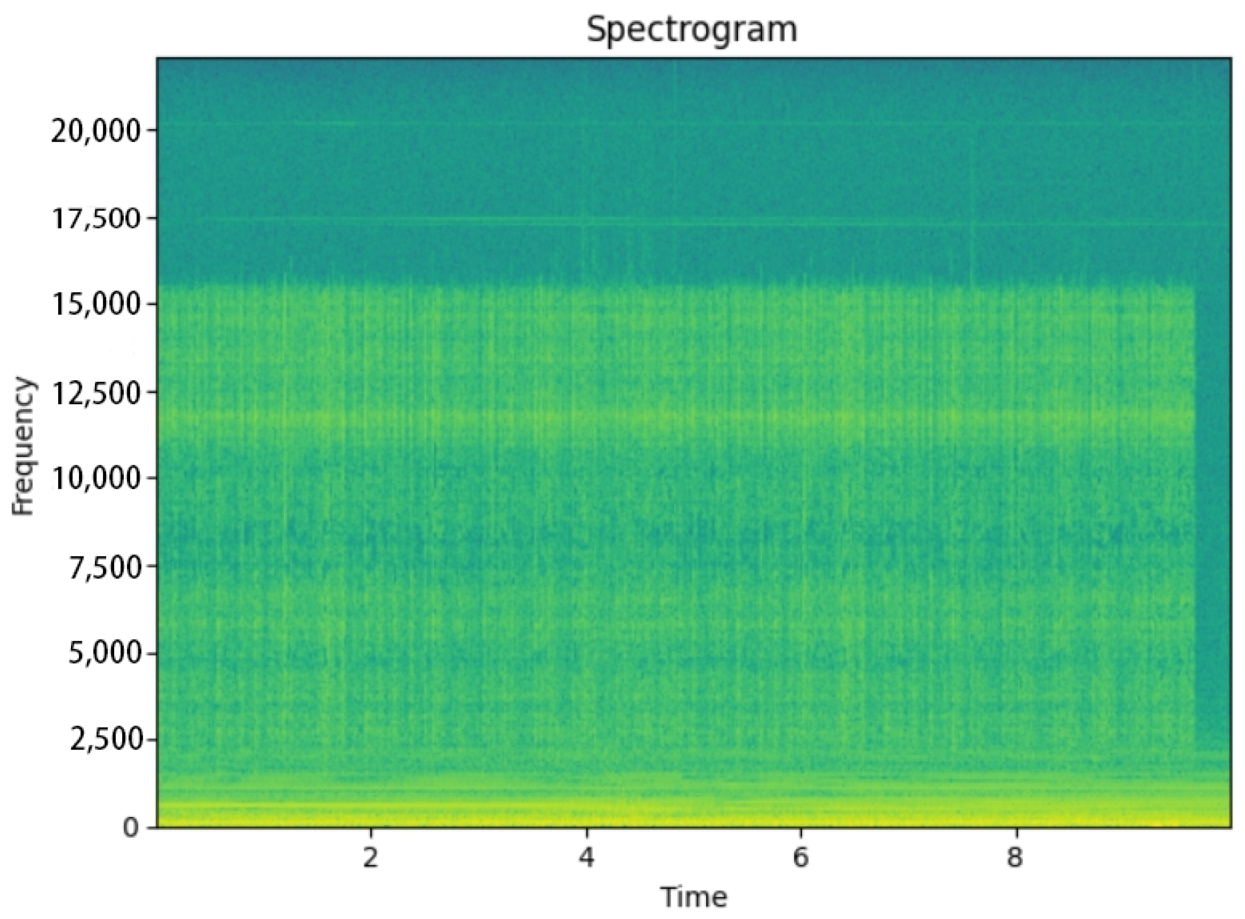
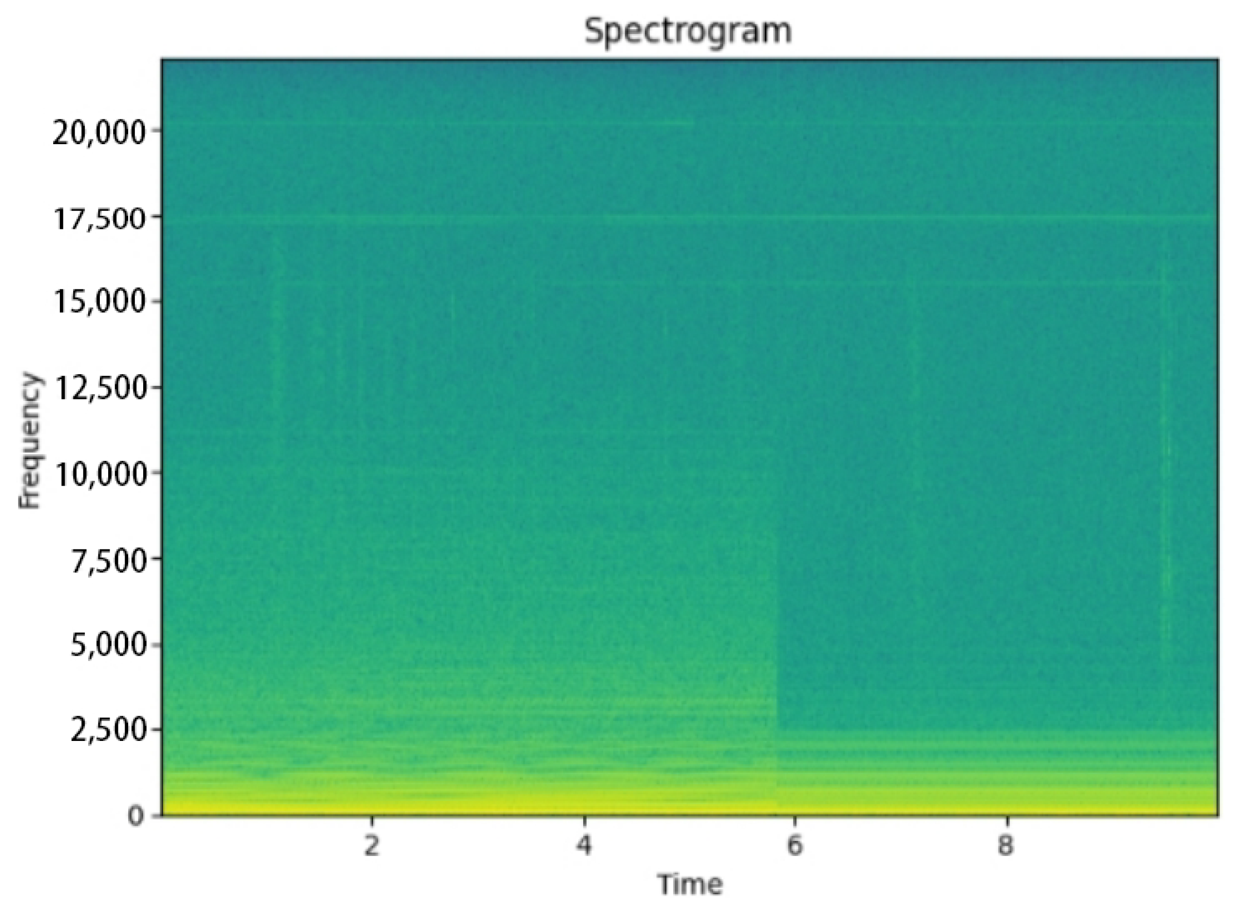
2.2. Grammatic Analysis

Figure 4, Figure 5 and Figure 6 show the spectrogram of the transformer during normal operation, discharge, and overload. In contrast to the waveform graph, which is represented by a single time domain, the spectrogram is a representation of sound in the time-frequency domain that expresses deeper voiceprint characteristics while also fully describing the frequency and speech energy information in the direction of time. This is advantageous for the model’s full learning process [21]. The color represents the intensity of sound at a particular frequency and moment, with yellow representing high intensity and green representing low intensity. The spectrogram’s horizontal and vertical axes represent frequency and time in seconds, respectively. The spectrogram shows the composition of the spectrum from three dimensions, has the characteristics of sound data representation and image form processing, and uses two-dimensional images to express three-dimensional information. Assuming that the speech waveform time-domain signal is $x(l)$, the spectrogram calculation formula is

$$x_n(m)=W(m)x(n+m),1\le m\le P$$

(1)

$$X_n(e^{jw})={\displaystyle \sum _{m=1}^P}{x}_n(m)e^{-jwm}$$

(2)

$$w=2\pi k/P$$

(3)

$$X_n(e^{\frac{2\pi kj}{P}})=X_n(k)={\displaystyle \sum _{m=1}^P}{x}_n(m)e^{\frac{-2\pi jkm}{P}},1\le k\le P$$

(4)

$$T(n,k)=|X_n{(k)|}^2,$$

(5)

where $x_n(m)$ is the nth frame sound signal obtained after framing the window, $W(m)$ is the window function, $X_n(e^{jw})$ is a short-term Fourier change of the framed signal, w is the angular frequency, P is the number of Fourier conversion points, $|X_n(k)|$ is a short-term amplitude spectrum estimate of $x_n(m)$, and $T(n,k)$ is the spectral energy density function at time. $T(n,k)$ is a nonnegative real matrix, with time n as the abscissa and k as the ordinate. A heat map can be drawn, and a color spectrogram can be derived from the transformed matrix fine image and color mapping. The ordinate of the spectrogram represents the frequency in $(HZ)$. The abscissa represents the time in $(S)$.

The figure demonstrates that the frequency range of the sound when the transformer is discharged covers the high-frequency band, whereas the sound during normal operation is primarily concentrated in the low-frequency band. When the transformer is overloaded, it can be seen that in the range of low- and medium-frequency bands, the intensity of the sound is greater than the sound intensity during normal operation. From the time and frequency domain analysis, it is feasible to use sound signals for abnormal transformer diagnosis.

3. Preprocessing and Feature Extraction of Sound Signals

3.1. Preprocessing of Sound Signals

By preprocessing the sound, the effects of aliasing, high-order harmonic distortion, high frequency, and other issues on the energy and frequency of the sound signal can be eliminated [21]. Additionally, high-quality parameters can be input for the subsequent feature extraction step, enhancing the effect of sound signal feature extraction.

Although the same device is used to collect samples, due to various factors, there are also many differences between the individual sound samples collected. In order to narrow the impact of these differences on sound quality, the data must first be normalized as

$$Y_{nom}=\frac{X-X_{min}}{X_{max}-X_{min}},$$

(6)

where $X_{min}$ and $X_{max}$ are the minimum and maximum values of the sound signal.

Any sound signal must be analyzed and processed by using “short-time”, or “short-time analysis”, because the sound signal is thought to be stable for a short time. As a result, the sound signal is framed. In voiceprint detection, the frame length will lead to poor representation of the feature vector, and too long a length will affect the accuracy of the feature vector, so generally take 20–30 ms as a frame [18]. This paper takes 25 ms as a frame and the frame shifts to 10 ms. In order to ensure the continuity between adjacent frames, the overlapping part between the two frames is set up, and the relationship between the overlapping part and the frame signal is

$$M=l-Lb/\left[L\left(1-b\right)\right],$$

(7)

where the number of frames is M, l is the length of the sound signal, L is the frame length, and b is the overlap rate.

In order to facilitate the calculation and make the sound have good continuity, the overlap rate is 30% in this article. After framing the sound, a discrete Fourier transform is required, and directly transforming the sound signal will cause signal distortion. Therefore, a Hamming window must be added to the frame signal to increase continuity at both ends and make the low-pass characteristics smoother and less distorted. The Hamming function is

$$W\left[l\right]=0.54-0.64cos(2\pi l/(Z-1)),0\le l\le Z-1,$$

(8)

where Z is the window length.

3.2. Feature Extraction of Sound Signals

A cepstral parameter derived from the Mel scale frequency domain is the MFCC coefficient. It involves the nonlinear properties of the frequency that the human ear hears [22]. The following equation can approximate the MFCC coefficient’s relationship to frequency,

$$B(h)=2595lg(1+\frac{h}{700}),$$

(9)

where B is the Mel frequency and h is the frequency.

The first-order differences and second-order differences of the MFCC coefficients can reflect the variability of adjacent frames, so this paper uses the MFCC coefficient combined with the difference as the feature vector of the sound signal. Figure 7 depicts the process flow of feature extraction.

In most cases, the signal is transformed into an energy distribution in the frequency domain by using a fast Fourier transform (FFT) for characteristic observation because it is challenging to observe the signal’s characteristics in the time domain. FFT conversion is performed on each preprocessed sound signal, and the calculation formula is:

$$F_a(q)={\displaystyle \sum _{n=0}^{P-1}}S(n)e^{-2\pi iq/P},0\le q\le P,$$

(10)

where $S(n)$ is the input sound signal, and P is the number of Fourier conversion points. Here, take 512. After FFT transformation of the framed signal, and then Mel filtering, Mel filtering is achieved by a filter bank composed of multiple triangle bandpass filters. Set the number of filters to p, and then set the sound signal after Mel filtering to obtain p parameters $m_i(i=1,2,...,p)$, and the calculation formula is

$$m_i=ln({\displaystyle \sum _{q=0}^{P-1}}\left|F_a(q)\right|\times H_i(q)),i=1,2,...,p,$$

(11)

where $H_i(q)$ is the parameter of the filter, which could be summed up as

$$\left\{\begin{array}{cc}0,\hfill & \hfill q\le f(c-1)\\ \frac{2(q-f(c-1))}{(f(c+1)-f(c-1))(f(c)-f(c-1))},\hfill & \hfill f(c-1)\le q\le f(c)\\ \frac{2(f(c+1)-q)}{(f(c+1)-f(c-1))(f(c+1)-f(c))},\hfill & \hfill f(c)\le q\le f(c+1)\\ 0,\hfill & \hfill q\ge f(c+1),\end{array}\right.$$

(12)

where $f(c)$ is the center frequency of the triangulation filter. According to the calculation of $m_i$, take the logarithm to perform a discrete cosine transformation, and the transformation formula is

$$c(i)=\sqrt{\frac{2}{P}}{\displaystyle \sum _{j=1}^p}{m}_{j}cos\left[(j-0.5)\frac{\pi i}{p}\right],1\le i,j\le p$$

(13)

where $c(i)$ is the MFCC feature of the frame signal, and it is combined into a first-order and second-order differential as the feature vector of the frame signal.

4. Construction of CNN-LSTM Hybrid Model Based on Attention Mechanism

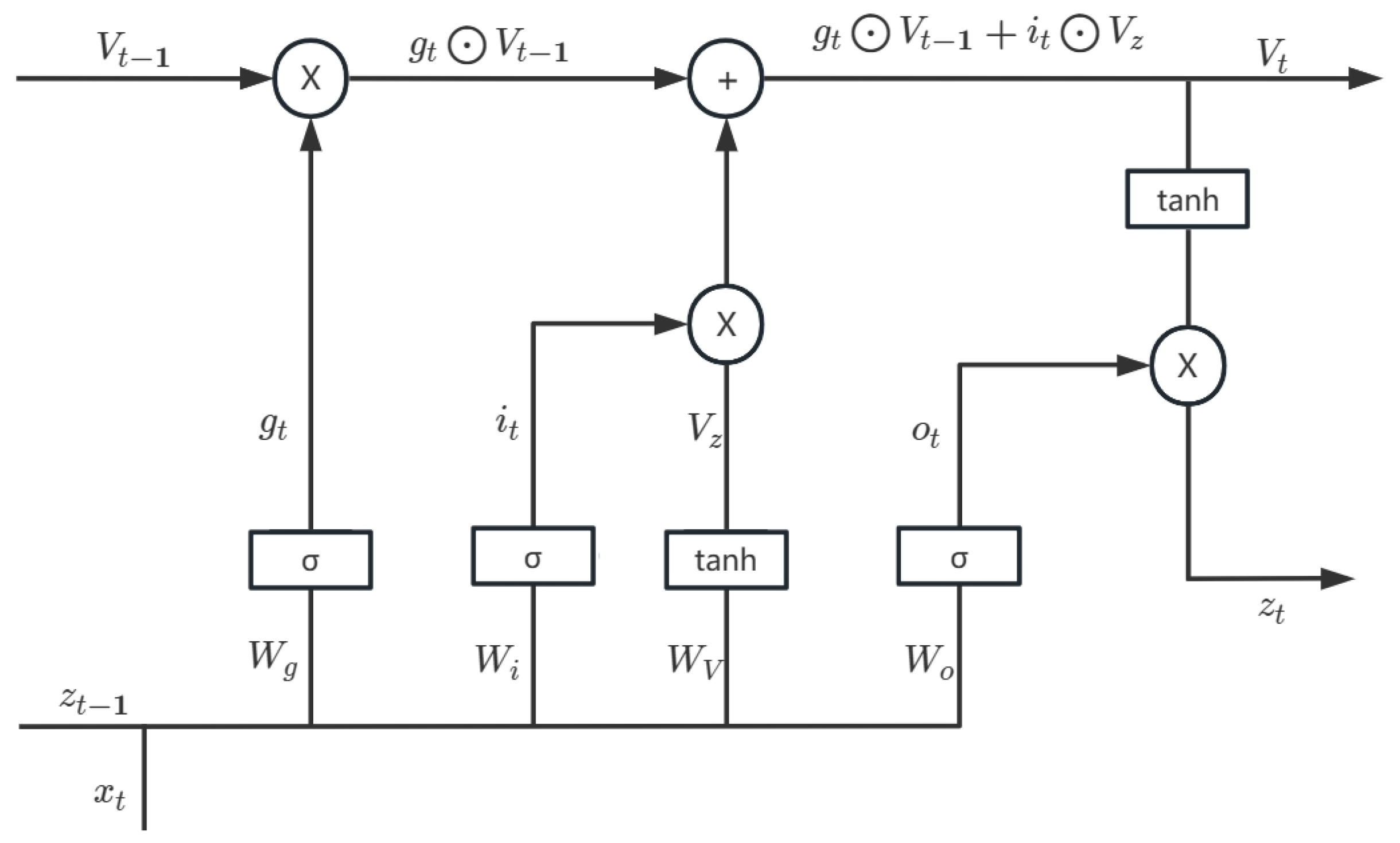
4.1. Long Short-Term Memory

Long short-term memory (LSTM) is a unique RNN type of memory. LSTM adds gating devices, which can remember information through cell state. The forgetting gate can avoid letting too many memories affect the neural network’s processing of the current input, and each time a new input is entered—based on the latest moment’s input and output—the LSTM will first select which previous memories to erase. A memory gate is a control unit that determines whether the data at t (now) is included in the state. It can filter out invalid data from the current input and extract valid data from it. The neural layer that the LSTM unit uses to determine the current value of the output is the output gate. After integrating the current input value with the output value of the moment before it with the sigmoid function, the output layer will first extract the information from the vector, and then use the tanh function compression to map the current unit state to the interval $(-1,1)$. LSTM introduces the sigmoid function through its three gatings and combines it with the tanh function to increase the summation steps, reduce the possibility of gradient vanishing and gradient explosion, and solve both short-term and long-term dependence problems [23,24,25,26]. The structure of the LSTM element is shown in Figure 8, and its calculation formula is show in Equations (14)–(19),

$$g_t=\sigma (W_g·[z_{t-1},x_t]+b_g)$$

(14)

$$i_t=\sigma (W_i·[z_{t-1},x_t]+b_i)$$

(15)

$$V_t=\sigma (g_t·V_{t-1}+i_t·V_z)$$

(16)

$$V_z=tanh(W_V·[z_{t-1},x_t]+b_V)$$

(17)

$$o_t=\sigma (W_o·[z_{t-1},x_t]+b_o)$$

(18)

$$z_t=o_t\ast tanh(V_t)$$

(19)

where $x_t$ is the network input matrix, and $\sigma$ is the activation function. $V_{t-1}$ is the old cell state, updated to the new cell state $V_t$ by Equation (16). $tanh$ is the double tangent activation function, $(W_g,W_i,W_V,W_o)$ is the parameter of the network model, and $(b_g,b_i,b_V,b_o)$ is the offset vector of the network. The model updates the weights and biases by minimizing the objective function.

4.2. Convolutional Neural Networks

CNN is one of the most widely used neural networks for image recognition, pattern recognition, feature extraction, and natural language processing. The convolutional layer, pooling layer, fully connected layer, and softmax layer make up CNN’s network structure, which is a feedforward neural network with deep structure and convolutional operation [24]. The functions of its layer structure are as follows.

The convolutional layer is the heart of the convolutional neural network. It abstracts the implied correlation in the input data by using the convolutional kernel matrix and extracts features. Each layer’s convolution operation is carried out with a rectified linear unit (ReLU) activation function [27] in the following ways:

$$f(x)=max(0,x).$$

(20)

After the completion of the activation function process, the filter generates the following characteristics,

$$y_j^l=f({\displaystyle \sum _{i\in M_j}}{x}_i^{l-1}\ast w_{ij}^l+b_j^l),$$

(21)

where, in the convolutional layer, j, $y_j^l$ is the result of the l filter, f represents the nonlinear function, operator * represents convolution, $w_{ij}^l$ is the lth layer convolution kernel between the i input map and the j output map, and $b_j^l$ is the bias.

With regard to the pooling layer, the convolutional layer extracts a large number of features of the input data, and the calculation efficiency is relatively low when performing feature operations, so it is necessary to solve this problem through the pooling layer. The pooling layer is responsible for screening the features in the sensory domain and extracting the most representative features in the region. This can effectively reduce the output feature’s dimension and the number of required model parameters. Pooling is divided into average pooling and maximum pooling. Average pooling can keep more background information about the object and reduce the excessive variance in the estimated value caused by neighborhood limitations. Maximum pooling, on the other hand, can keep more texture information about the object while reducing the estimated mean shift caused by convolutional layer parameter error. This article uses voiceprint information for transformer condition monitoring, so the method of maximum pooling is used.

The model’s final layer is the fully connected layer, which connects each neuron with the neurons before and after it is used and calculates the weight and deviation of the features to obtain the output of feature information.

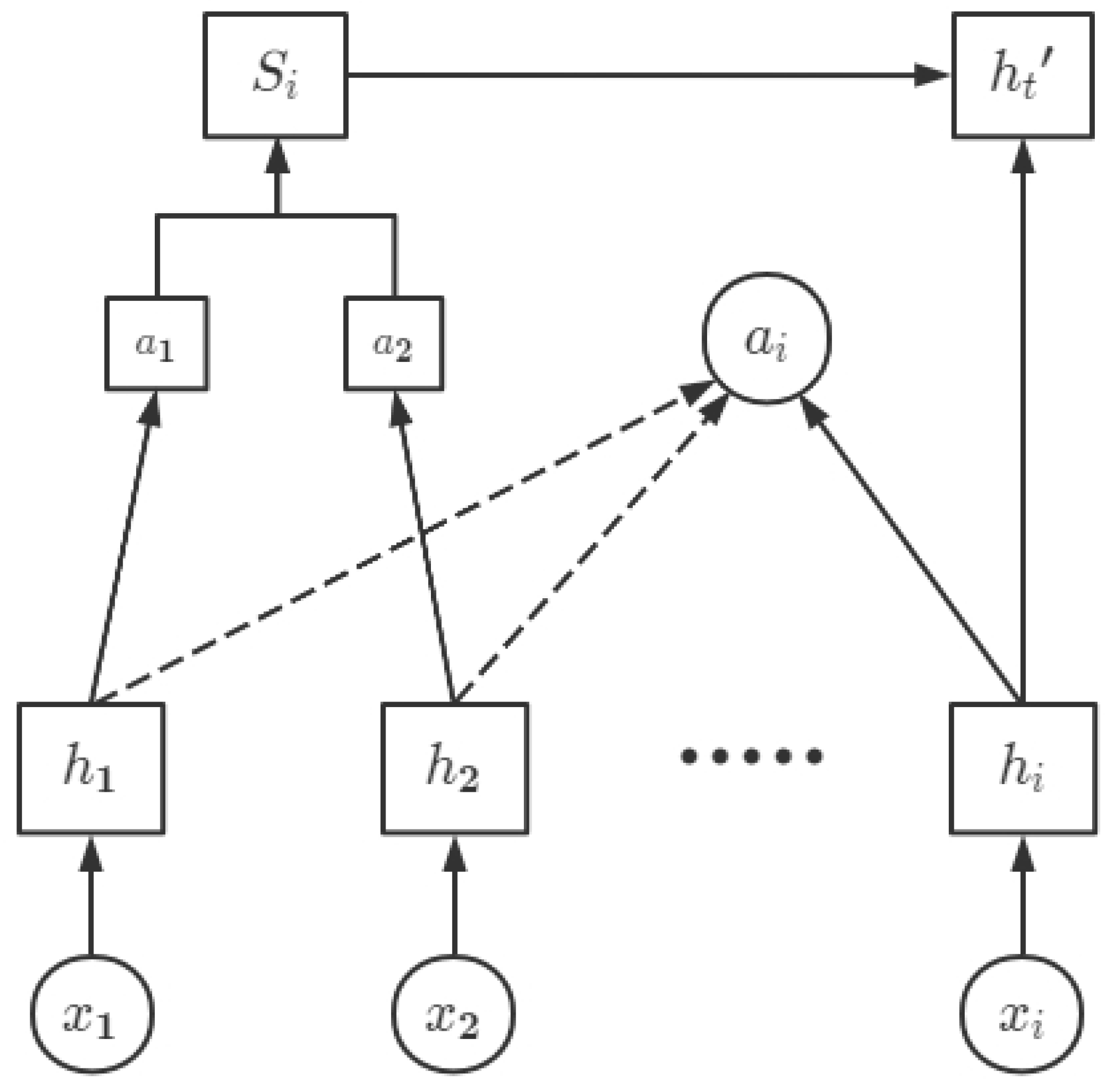
4.3. Attention Mechanism

The ability to selectively select significant information from a large amount of information is at the heart of the attention mechanism, capture important information useful for the current task, highlight important features that affect the impact, reduce the impact of useless features, make the model make the optimal choice, and improve the accuracy of the model. Its pith is to gain proficiency with a weight dissemination of information highlights and afterward apply this weight conveyance to the first elements so the undertaking principally centers around a few key highlights, disregards irrelevant highlights, and further develops task effectiveness [28], the design of the consideration component is displayed in figures [29,30,31]:

In Figure 9, $x_1,x_2,...,x_i$ is the input feature value, $h_1,h_2,...,h_i$ is the input feature-specific hidden layer state value, and $a_t$ is the weight value of the current input that is equivalent to the state of the historical input’s hidden layer. $h_t^{\prime }$ is the value of the hidden layer’s state that the final node outputs. The attention mechanism is calculated as

$$e_i=utanh(w{h}_i+b)$$

(22)

$$a_i=\frac{exp(e_i)}{{\sum }_{t=1}^{n}exp(e_t)}$$

(23)

$$s_i=\sum _{t=1}^n{e}_i{a}_i,$$

(24)

where w and b are the weight parameters and biases, $e_i$ is the attention probability distribution value determined by the input vector $h_i$ at the i moment, and $s_i$ is the feature of the final output.

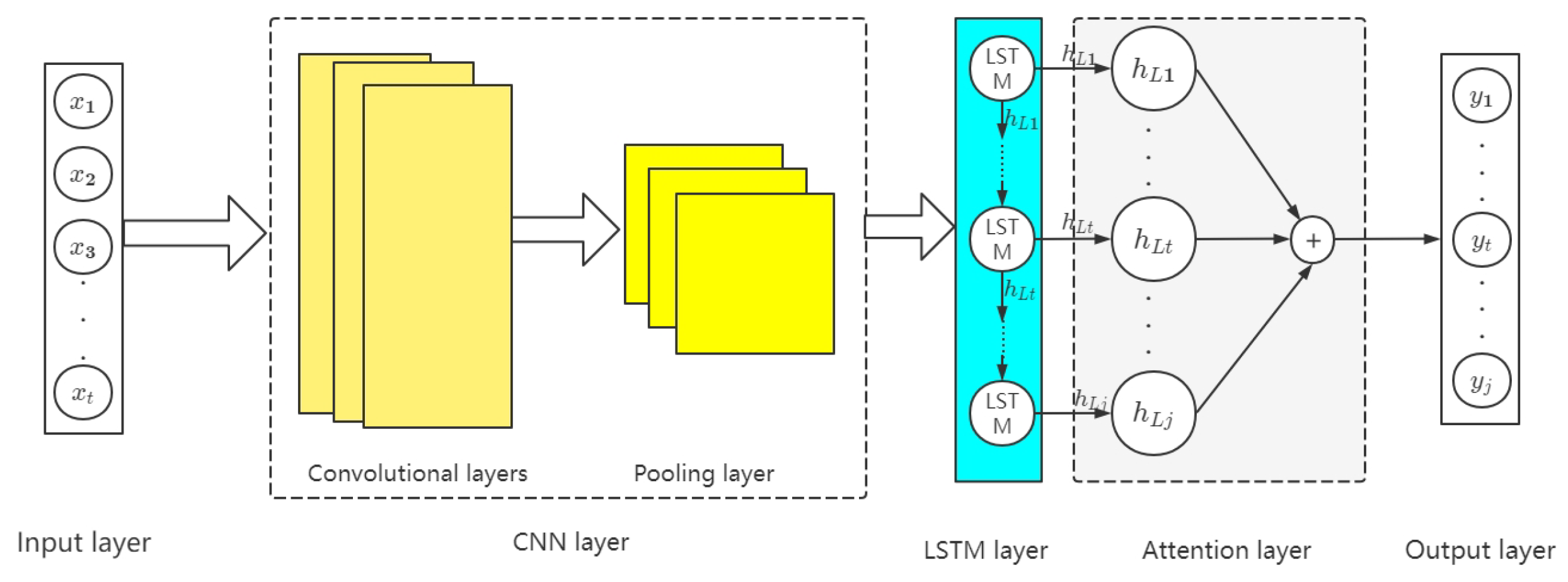
4.4. CNN-LSTM Hybrid Model Based on Attention Mechanism

The feature vector composed of voiceprint signals after feature extraction cannot reflect the potential relationship between features, so the CNN network is used to mine the potential relationship between features, extract the rules between continuous data and discontinuous data, and form vectors, and then pass them into the LSTM layer in chronological order to capture long-term components. However, the CNN-LSTM model may lose data if the time series data is input for an excessive amount of time. Additionally, the CNN-LSTM model only takes into account the selection of input features and does not take into account the impact of any one feature on the results. As a result, the attention mechanism is used in this paper to add various weights to the model’s input features, enhance the features that have a greater impact on the results, and suppress the features that have a small impact on the results.

As can be seen in Figure 10, the input layer, the CNN layer, the LSTM layer, the attention layer, and the output layer make up the majority of the CNN-LSTM hybrid model that is based on the attention mechanism.

The hybrid model structure and flow are as follows:

• Input layer: The MFCC features of the sound samples after feature extraction is passed into the model through the input layer. If the input length is t, $X=[x_1,x_2,...,x_t]$ can be used to represent the input direction.
• CNN layer: The CNN layer mainly includes the convolutional layer and the pooling layer, which is to feature further extraction of the feature vector input of the input layer and extract and screen out the important feature vectors into the LSTM layer. According to the data structure of the voiceprint sample, this paper uses two-dimensional convolution, the convolution kernel is 9, and the activation function is ReLU. In order to retain more features, this paper uses the maximum pooling, and the pool size is 2. After the CNN layer processes the input vector, the incoming fully connected layer is transformed into a new feature vector (26). The output of the CNN layer is $H_C={[h_{C1},h_{C2},...,h_{Ci}]}^T$, and the calculation formula is

  $$C=ReLU(X\otimes W_C+b_C)$$

  (25)

  $$P=max(C)+b_P$$

  (26)

  $$H_C=f(W_H·P+b_H),$$

  (27)

  where C is the convolutional layer’s output, $W_C$ and $b_C$ are the weights and biases of the convolutional layer, respectively, ⊗ is the convolution operator, P is the pooling layer’s output, $max$ is the maximum pooling mode, and $b_P$ is the bias of the pooling layer. The fully connected layer’s activation function is called f. The fully connected layer’s weights and biases are $W_H$ and $b_H$.
• LSTM layer: To understand how the data feature time series are related, the CNN layer passes the extracted feature vectors onto the LSTM layer. In this paper, the LSTM structure of bidirectional transmission is adopted, and the number of hidden units in each layer is 120. The activation function is the RULE function, and the LSTM layer’s output vector is $H_L={[h_{L1},h_{L2},...,h_{Li}]}^T$.
• Attention layer: In accordance with the weight distribution principle, we input the vector output of LSTM into the attention layer and assign distinct parameters to distinct characteristic parameters to create the ideal weight parameter matrix. The output of this layer is $S={[s_1,s_2,...,s_k]}^T$.
• Output layer:The output from the attention layer goes into the output layer, which then sends the status data for the transformer through the full connection layer. The output is Y, and the following formula calculates it as

  $$Y=f(W_Y·S+b_Y),$$

  (28)

  where $W_Y$ and $b_Y$ are the weights and biases of the output layer.

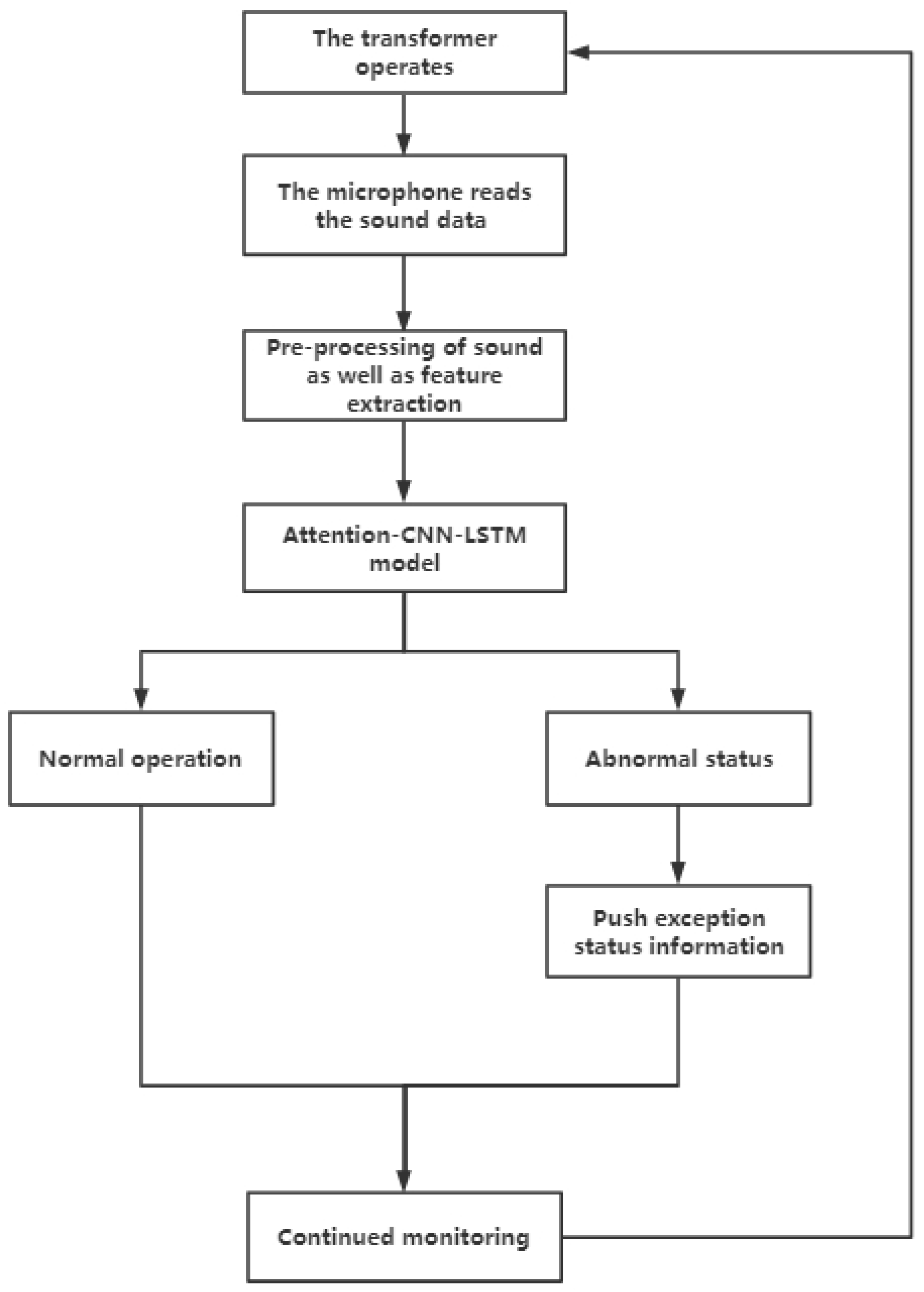
4.5. Real-Time Transformer Condition Monitoring Process

The normal operation is diagnosed by using the Attention-CNN-LSTM hybrid model in this paper, discharge and overload of the transformer running in real time, and the overall diagnostic flow chart is shown in Figure 11.

The specific steps for detection are as follows.

• The sound of the transformer operation is collected in real time through the microphone and converted into data.
• Preprocess the data collected by the microphone and extract MFCC features to form a feature vector.
• Input feature vectors into the trained Attention-CNN-LSTM model for discrimination.
• If the discrimination result is normal, continue monitoring. If the discrimination result is the abnormal state (discharge, overload), push the abnormal information and occurrence time, and continue monitoring.

5. Analysis of Experimental Results

In order to evaluate the Attention-CNN-LSTM model’s superiority and accuracy in comparison to three other prevalent detection and classification models—CNN, LSTM, and CNN-LSTM—we set them up for comparative analysis. The results are further analyzed by using the confusion matrix, which intuitively shows the impact of these four models for normal, discharge, and the detection effect of these three states of overload.

5.1. Model Training Settings

5.1.1. Sample Settings

The sound samples are divided into 2-s units, the samples of the three states in the quiet environment and the three state samples under the loud ambient sound are randomly sorted in order and then put into the model for training in turn, and the training set and the test set are randomly divided into 8:2 ratio, and the number of samples in each environment is shown in

Table 1. Number of sound samples for each condition of 110-kV transformer.

State	Quiet Environment/pcs	Thunderstorm Environment/pcs	Fan Environment/pcs
Normal operation	125	60	75
Overload	75	35	50
Discharge	70	40	45

.

5.1.2. Evaluate the Performance Index Settings

The confusion matrix M, precision ratio (P), recall (R), and F1-score ($F1$) are all utilized in the process of assessing the model’s detection performance, where precision is the expected outcome of the label sample, which is actually the proportion of the label. The recall rate is the proportion of the label that is actually the sample of the label, and the predicted result is the proportion of the label. F1 is defined based on the harmonic average of accuracy and duplicate check rate. The specific evaluation formula is as follows [32,33],

$$M=\left[\begin{array}{cc}{y}_{TP}& y_{FP}\\ y_{FN}& y_{TN}\end{array}\right]$$

(29)

$$P=\frac{y_{TP}}{y_{TP}+y_{FP}}$$

(30)

$$R=\frac{y_{TP}}{y_{TP}+y_{FN}}$$

(31)

$$F1=\frac{2\times P\times R}{P+R},$$

(32)

where $y_{TP}$ is the number of data points whose actual abnormal state data points are detected as abnormal points. The number of data points that are found to be normal in the actual abnormal state is $y_{FN}$. The number of data points identified as abnormal by actual normal operation is $y_{FP}$; $y_{TN}$ is the number of data points that are detected as normal data points in actual normal operation.

P and R can intuitively show the quality of normal points and abnormal points detected by the hybrid model through percentages, P and R are proportional to the performance of the detection model when evaluating the performance of the detection model, and when P and R are high, the F1 value will be high. The value of $F1$ has perfect precision and recall at a value of 1, and its worst value is 0.

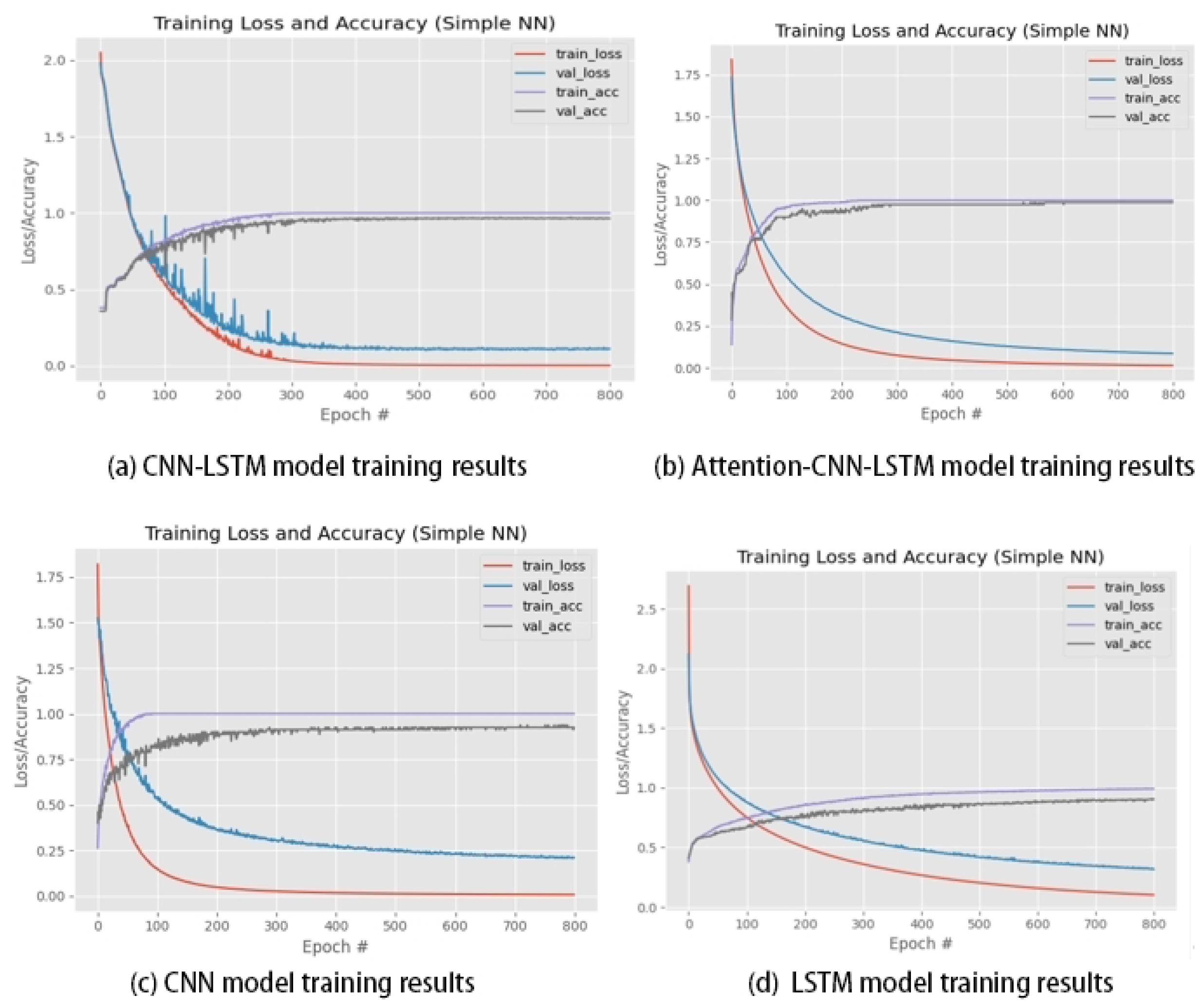
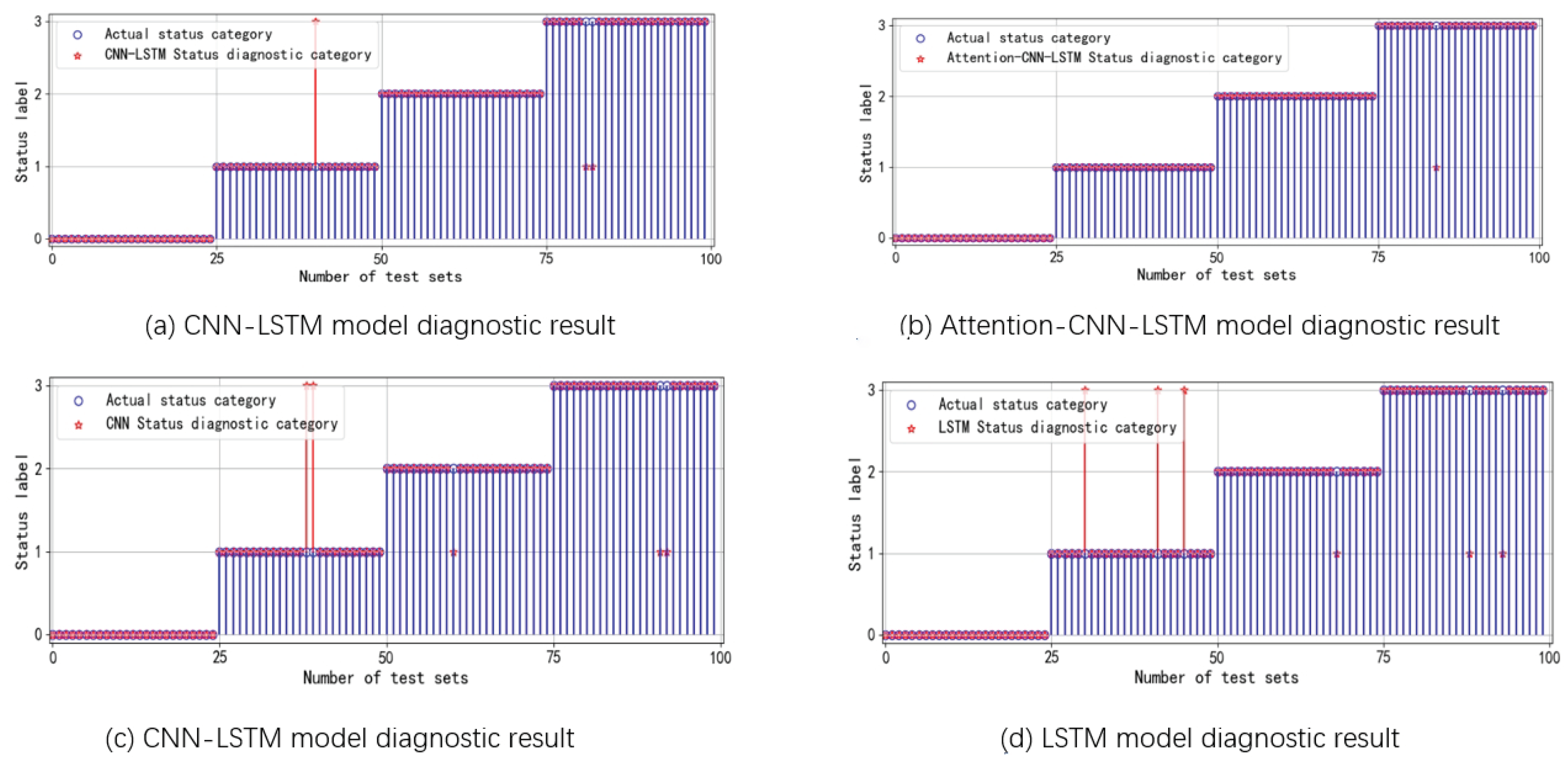
5.2. Detection Performance Analysis

One needs to train the model after setting the samples and the evaluation indicators. One needs to set the number of iterations of the model to 800, the number of batch samples to 64, the loss function to MSE, and the optimizer to Adam. You then need to put the training samples into the model for training and the test samples into the model for testing. The four results of training the model are shown in Figure 12.

From the figure, Figure 12a is the CNN-LSTM model training results, Figure 12b is the Attention-CNN-LSTM model training results, Figure 12c is the CNN model training results, and Figure 12d is the LSTM model training results. It can be seen that the accuracy (train_acc) of the four models on the training set can reach 100%, but the accuracy (val_acc) on the test set is quite different. The Attention-CNN-LSTM hybrid model can reach 99.7% accuracy on the test set, the accuracy of the CNN-LSTM hybrid model reaches 97%, and the accuracy of the CNN model and the LSTM model on the test set is 90% and 92%, respectively.

From the Figure 13, Figure 13a is the CNN-LSTM model status diagnostic results, Figure 13b is the Attention-CNN-LSTM model status diagnostic results, Figure 13c is the CNN model status diagnostic results, and Figure 13d is the LSTM model status diagnostic results. In this experiment, 25 test sets were randomly selected from the samples of the four states, 0 represents the ambient noise state when the transformer is not started, 1 represents the normal operation of the transformer, 2 represents the partial discharge state of the transformer, and 3 represents the overload state of the transformer. From the experimental results, it can be seen that the CNN-LSTM model identifies a sample in normal operation state and overload state as overload state and normal operation state respectively. The Attention-CNN-LSTM model only identifies an overloaded sample as a normal operating state. The CNN model identifies two samples in normal operation as overload, two samples in overload as normal operation and one partial discharge sample as normal operation. The LSTM model identifies three samples of normal operation as overload, one partial discharge as normal operation, and two overload samples as normal operation.

The above experimental results show that Attention-CNN-LSTM has a smaller loss in the test set and the highest accuracy in the random test set, so the training effect and accuracy of the Attention-CNN-LSTM hybrid model are the best among the four models. The evaluation parameters for the detection performance of the four models are shown in

Table 2. Parameters of performance evaluation.

Model	State	Precision	Recall	F1-Score
Attention-CNN-LSTM	Normal operation	99.6%	99.8%	0.997
	discharge	99.8%	99.8%	0.998
	overload	99.2%	99.4%	0.993
CNN-LSTM	Normal operation	96.4%	97.6%	0.97
	discharge	98.2%	98.8%	0.985
	overload	96.2%	97.2%	0.967
CNN	Normal operation	90.5%	91.3%	0.909
	discharge	91.4%	92.2%	0.918
	overload	90.2%	90.3%	0.902
LSTM	Normal operation	92.6%	91.8%	0.922
	discharge	93.4%	93.6%	0.935
	overload	91.3%	91.5%	0.914

.

The table demonstrates that, in terms of detecting the three states of the transformer on precision, recall, and F1, the Attention-CNN-LSTM hybrid model performs best, with an accuracy that can exceed 99%, followed by the CNN-LSTM hybrid model. Among these four models, the CNN model and the LSTM model perform poorly. Due to the continuity of timeline and space of voiceprint features, a single model has limitations in voiceprint detection, resulting in unsatisfactory detection results.

In summary, the Attention-CNN-LSTM hybrid model has the highest detection performance, which can provide auxiliary decision-making for the real-time detection of transformers and provide a reference for reducing the losses caused by transformers and the abnormal detection of electrical equipment.

6. Discussion and Conclusions

The production and life processes will generate a significant amount of data once we enter the era of big data. Neural networks and artificial intelligence have been used in equipment monitoring to ensure work efficiency, effectively reducing the need for human resources and increasing the accuracy of equipment diagnosis [34]. Sound, as one of the most critical characteristics of equipment operation, contains a lot of information about how the equipment is used. This paper, through the collection of transformer sound in the real scene combined with deep learning in the field of the voiceprint, proposed a transformer anomaly diagnosis method based on the Attention-CNN-LSTM hybrid model. We input the feature vector of sound samples, through the Attention-CNN-LSTM hybrid model for feature learning training, and achieved high accuracy. Therefore, combining sound and deep learning to monitor equipment operating status may become a future research direction in the field of voiceprint recognition.

References

1. Li, G.; Yu, C.; Liu, Y.; Fan, H.; Wen, F.; Song, Y. Power transformer fault prediction and health management: Challenges and prospects. Power Syst. Autom. 2017, 41, 156–167. [Google Scholar]
2. Hussain, M.R.; Refaat, S.S.; Abu-Rub, H. Overview and partial discharge analysis of power transformers: A literature review. IEEE Access 2021, 9, 64587–64605. [Google Scholar] [CrossRef]
3. Duval, M. The duval triangle for load tap changers, non-mineral oils and low temperature faults in transformers. IEEE Electr. Insul. Mag. 2008, 24, 22–29. [Google Scholar] [CrossRef]
4. Duval, M. New techniques for dissolved gas-in-oil analysis. IEEE Electr. Insul. Mag. 2003, 19, 6–15. [Google Scholar] [CrossRef]
5. Ghoneim, S.S.; Taha, I.B. A new approach of DGA interpretation technique for transformer fault diagnosis. Int. J. Electr. Power Energy Syst. 2016, 81, 265–274. [Google Scholar] [CrossRef]
6. Amora, M.A.B.; Almeida, O.d.M.; Braga, A.P.d.S.; Barbosa, F.R.; Lisboa, L.; Pontes, R. Improved DGA method based on rules extracted from high-dimension input space. Electron. Lett. 2012, 48, 1048–1049. [Google Scholar] [CrossRef]
7. Kim, S.W.; Kim, S.J.; Seo, H.D.; Jung, J.R.; Yang, H.J.; Duval, M. New methods of DGA diagnosis using IEC TC 10 and related databases Part 1: Application of gas-ratio combinations. IEEE Trans. Dielectr. Electr. Insul. 2013, 20, 685–690. [Google Scholar]
8. Mansour, D.E.A. Development of a new graphical technique for dissolved gas analysis in power transformers based on the five combustible gases. IEEE Trans. Dielectr. Electr. Insul. 2015, 22, 2507–2512. [Google Scholar] [CrossRef]
9. Li, X.; Wu, H.; Wu, D. DGA interpretation scheme derived from case study. IEEE Trans. Power Deliv. 2010, 26, 1292–1293. [Google Scholar] [CrossRef]
10. Soni, R.; Chaudhari, K. An approach to diagnose incipient faults of power transformer using dissolved gas analysis of mineral oil by ratio methods using fuzzy logic. In Proceedings of the 2016 International Conference on Signal Processing, Communication, Power and Embedded System (SCOPES), Odisha, India, 3–5 October 2016; IEEE: Piscataway, NJ, USA, 2016; pp. 1894–1899. [Google Scholar]
11. Seo, J.; Ma, H.; Saha, T.K. A joint vibration and arcing measurement system for online condition monitoring of onload tap changer of the power transformer. IEEE Trans. Power Deliv. 2016, 32, 1031–1038. [Google Scholar] [CrossRef]
12. Min, L.; Huamao, Z.; Annan, Q. Voiceprint Recognition of Transformer Fault Based on Blind Source Separation and Convolutional Neural Network. In Proceedings of the 2021 IEEE Electrical Insulation Conference (EIC), Virtual, 7–28 June 2021; IEEE: Piscataway, NJ, USA, 2021; pp. 618–621. [Google Scholar]
13. Wang, S.; Zhao, B.; Du, J. Research on transformer fault voiceprint recognition based on Mel time-frequency spectrum-convolutional neural network. In Proceedings of the Journal of Physics: Conference Series; IOP Publishing: Bristol, UK, 2022; Volume 2378, p. 012089. [Google Scholar]
14. Dang, X.; Wang, F.; Ma, W. Fault Diagnosis of Power Transformer by Acoustic Signals with Deep Learning. In Proceedings of the 2020 IEEE International Conference on High Voltage Engineering and Application (ICHVE), Beijing, China, 6–10 September 2020; IEEE: Piscataway, NJ, USA, 2020; pp. 1–4. [Google Scholar]
15. Yu, Z.; Li, D.; Chen, L.; Yan, H. The research on transformer fault diagnosis method based on vibration and noise voiceprint imaging technology. In Proceedings of the 2019 14th IEEE Conference on Industrial Electronics and Applications (ICIEA), Xi’an, China, 19–21 June 2019; IEEE: Piscataway, NJ, USA, 2019; pp. 216–221. [Google Scholar]
16. He, P.; Xu, H.; Yin, L.; Wang, L.; Zhu, L. Power Transformer Voiceprint Operation State Monitoring Considering Sample Unbalance. In Proceedings of the Journal of Physics: Conference Series; IOP Publishing: Bristol, UK, 2021; Volume 2137, p. 012007. [Google Scholar]
17. Gu, C.; Qin, Y.; Wang, Y.; Zhang, H.; Pan, Z.; Wang, Y.; Shi, Y. A transformer vibration signal separation method based on BP neural network. In Proceedings of the 2018 IEEE International Power Modulator and High Voltage Conference (IPMHVC), Jackson, WY, USA, 3–7 June 2018; IEEE: Piscataway, NJ, USA, 2018; pp. 312–316. [Google Scholar]
18. Wang, F.; Wang, S.; Chen, S.; Yuan, G.; Zhang, J. Transformer voiceprint recognition model based on improved MFCC and VQ. Proc. Chin. Soc. Electr. Eng. 2017, 37, 1535–1543. [Google Scholar]
19. Tossavainen, T. Sound Based Fault Detection System. Master’s Thesis, Aalto University, Espoo, Finland, 2015. [Google Scholar]
20. Negi, R.; Singh, P.; Shah, G.K. Causes of noise generation & its mitigation in transformer. Int. J. Adv. Res. Electr. Electron. Instrum. Eng. 2013, 2, 1732–1736. [Google Scholar]
21. Ye, F.; Yang, J. A deep neural network model for speaker identification. Appl. Sci. 2021, 11, 3603. [Google Scholar] [CrossRef]
22. Sahidullah, M.; Saha, G. A novel windowing technique for efficient computation of MFCC for speaker recognition. IEEE Signal Process. Lett. 2012, 20, 149–152. [Google Scholar] [CrossRef] [Green Version]
23. Shrestha, A.; Mahmood, A. Review of deep learning algorithms and architectures. IEEE Access 2019, 7, 53040–53065. [Google Scholar] [CrossRef]
24. Moradzadeh, A.; Mohammadi-Ivatloo, B.; Abapour, M.; Anvari-Moghaddam, A.; Gholami Farkoush, S.; Rhee, S.B. A practical solution based on convolutional neural network for non-intrusive load monitoring. J. Ambient Intell. Humaniz. Comput. 2021, 12, 9775–9789. [Google Scholar] [CrossRef]
25. Graves, A. Long short-term memory. In Supervised Sequence Labelling with Recurrent Neural Networks; Springer: Berlin/Heidelberg, Germany, 2012; pp. 37–45. [Google Scholar]
26. Wang, S.; Wang, X.; Wang, S.; Wang, D. Bi-directional long short-term memory method based on attention mechanism and rolling update for short-term load forecasting. Int. J. Electr. Power Energy Syst. 2019, 109, 470–479. [Google Scholar] [CrossRef]
27. LeCun, Y.; Bengio, Y.; Hinton, G. Deep learning. Nature 2015, 521, 436–444. [Google Scholar] [CrossRef]
28. Ju, Y.; Li, J.; Sun, G. Ultra-short-term photovoltaic power prediction based on self-attention mechanism and multi-task learning. IEEE Access 2020, 8, 44821–44829. [Google Scholar] [CrossRef]
29. Tay, N.C.; Tee, C.; Ong, T.S.; Teh, P.S. Abnormal behavior recognition using CNN-LSTM with attention mechanism. In Proceedings of the 2019 1st International Conference on Electrical, Control and Instrumentation Engineering (ICECIE), Kuala Lumpur, Malaysia, 25 November 2019; IEEE: Piscataway, NJ, USA, 2019; pp. 1–5. [Google Scholar]
30. Xiang, L.; Wang, P.; Yang, X.; Hu, A.; Su, H. Fault detection of wind turbine based on SCADA data analysis using CNN and LSTM with attention mechanism. Measurement 2021, 175, 109094. [Google Scholar] [CrossRef]
31. Liu, Y.; Liu, P.; Wang, X.; Zhang, X.; Qin, Z. A study on water quality prediction by a hybrid dual channel CNN-LSTM model with attention mechanism. In Proceedings of the International Conference on Smart Transportation and City Engineering 2021, Chongqing, China, 6–8 August 2021; SPIE: Bellingham, WA, USA, 2021; Volume 12050, pp. 797–804. [Google Scholar]
32. Zhang, W.; Dong, X.; Li, H.; Xu, J.; Wang, D. Unsupervised detection of abnormal electricity consumption behavior based on feature engineering. IEEE Access 2020, 8, 55483–55500. [Google Scholar] [CrossRef]
33. Stehman, S.V. Selecting and interpreting measures of thematic classification accuracy. Remote Sens. Environ. 1997, 62, 77–89. [Google Scholar] [CrossRef]
34. Nandi, S.; Toliyat, H.A.; Li, X. Condition monitoring and fault diagnosis of electrical motors—A review. IEEE Trans. Energy Convers. 2005, 20, 719–729. [Google Scholar] [CrossRef]
Figure 1. Normal state time domain waveform plot.
Energies 16 02151 g001
Figure 2. Discharge state time domain waveform plot.
Energies 16 02151 g002
Figure 3. Overload state time domain waveform plot.
Energies 16 02151 g003
Figure 4. Normal transformer spectrogram.
Energies 16 02151 g004
Figure 5. Discharge transformer spectrogram.
Energies 16 02151 g005
Figure 6. Overload transformer spectrogram.
Energies 16 02151 g006
Figure 7. The process of feature extraction.
Energies 16 02151 g007
Figure 8. LSTM unit structure.
Energies 16 02151 g008
Figure 9. Attention mechanism structure.
Energies 16 02151 g009
Figure 10. Attention CNN-LSTM model structure schematic.
Energies 16 02151 g010
Figure 11. The transformer monitors the overall flow chart in real time.
Energies 16 02151 g011
Figure 12. Four model training results.
Energies 16 02151 g012
Figure 13. Four model status diagnostic results.
Energies 16 02151 g013