Article

Discrete-Time Sliding Mode Current Control for a Seven-Level Cascade H-Bridge Converter

1
Laboratory of Power and Control Systems, Facultad de Ingeniería, Universidad Nacional de Asunción, Luque 2060, Paraguay
2
GRÉPCI Laboratory, École de Technologie Supérieure, Montreal, QC H3C 1K3, Canada
*
Author to whom correspondence should be addressed.
Energies 2023, 16(5), 2481; https://doi.org/10.3390/en16052481
Submission received: 11 December 2022 / Revised: 25 February 2023 / Accepted: 27 February 2023 / Published: 5 March 2023
(This article belongs to the Section F3: Power Electronics)

Abstract

:
This paper deals with the implementation and performance analysis of discrete-time sliding mode (DTSM) current control applied to a seven-level cascade H-bridge converter to track three-phase reference currents for a reactive load. The converter output voltages are synthesized using a modulation scheme based on phase-shifted carrier modulation. Simulation and experimental tests have been added to demonstrate the performance of the proposed controller. At the same time, the effectiveness of the DTSM is verified under transient and steady-state conditions, respectively, by measuring the total harmonic distortion and the mean square error.

1. Introduction

Power electronics is a discipline that is increasingly involved in all stages of electrical energy processing, such as generation, conversion, transmission, distribution, and conditioning in its different stages and forms (CA → CC, CC → CA, etc.). Nevertheless, power electronic converters are restricted in their operational capabilities by switching devices, the limitations of which are imposed by the physical characteristics of semiconductor materials. In this regard, much research is being carried out around developing new semiconductor switching devices with higher voltage withstand capabilities. However, the goal of increasing the operating voltage of converters with existing circuit breakers also finds its way with the introduction of multilevel converters.
Multilevel converters are very attractive for high-power motor drives and uninterruptible power system applications [1,2]. The main reason is that they offer low harmonic content [3], higher efficiency [4], and increased device utilization at low modulation indices [5], among other features. Well-established topologies in the industrial and research area are Neutral-Point-Clamped (NPC) [6,7], Flying Capacitor (FC) [8,9], and cascade H-bridge (CHB) [10]. The NPC converter has a simple design. However, as the number of voltage levels increases, the number of clamping diodes increases, as well as the complexity of voltage balance control [11,12,13]. The FC and NPC converters are quite similar, as long as the clamping diodes in NPC are replaced with floating capacitors. As the number of voltage levels increases, it requires many capacitors and a complicated voltage balance control [12,13,14]. The CHB converter, in particular, has the attractive feature of modularity and power scalability [15,16], voltage-level redundancies (or extra degrees of freedom) [17,18], and is more reliable compared to FC and NPC converters [19].
From the point of view of applied current controllers to CHB converters, some are already presented in the literature. Decoupled control based on PI is widely used in power quality improvement applications, e.g., for a five-level CHB STATCOM [20,21]. In [20], the gains of the PI controllers depend on the parameters of the filters. In [21], the response time reaches almost 40 ms and for a delta-connected seven-level CHB STATCOM, in [22] almost 10 ms. Furthermore, no robustness tests have been performed in any of these papers. The authors of [23,24] also used a PI as a current controller for a seven-level CHB STATCOM, and, in [25], for a 25-level version, and in [26], for a 45-level version. Although they obtained very good experimental results, the inner current controller is not their main contribution.
Lately, a fast dynamic response has been obtained with one of the most popular controllers, i.e., Model Predictive Control (MPC) variants. For a five-level CHB, the authors of [18] achieved a response time of 1 ms and reduced computational cost, and the authors of [27] proposed a long prediction horizon MPC, in which reference current tracking and common-mode voltage (CMV) minimization are achieved in a single optimization problem. In [28], an MPC is proposed as a current controller (inner loop) and a Sliding Mode Control (SMC) as a DC-link voltage regulator (outer loop). Despite all advantages of MPC, when this control is implemented in power converters, the free modulation becomes a disadvantage due to the unfixed switching frequency [29]. An interesting solution is shown in [30], for a seven-level CHB converter.
On the other hand, SMC is a nonlinear controller currently being applied to different systems and is mainly being studied in power electronics due to its simple implementation [31]. Most published articles refer to the application of this control technique (and some variants of it) to DC-DC converters [32,33], such as boost converters [34,35,36,37,38,39], buck converters [40,41,42], buck-boost converters [43], and, recently, to multiphase machines fed by DC-AC converters, such as two two-level voltage source converters [44,45] and matrix converters [46]. However, only a few publications are related to SMC applied to multilevel converters: NPC inverter [47] and modular multilevel converters (MMC) [48,49]. Then, there are no research studies about SMC applied to CHB as current controller, especially the seven-level version.
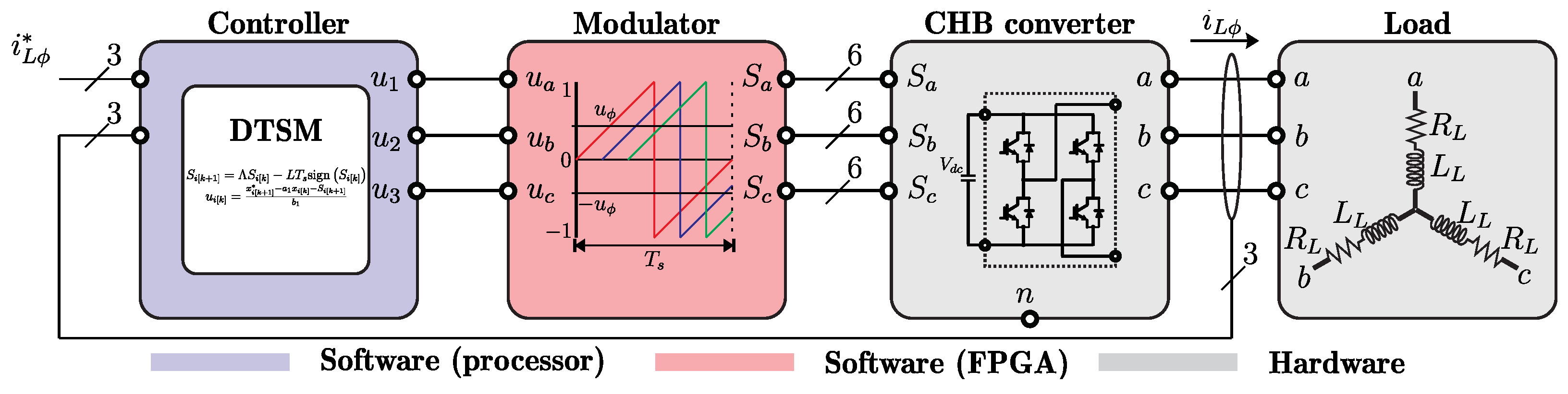
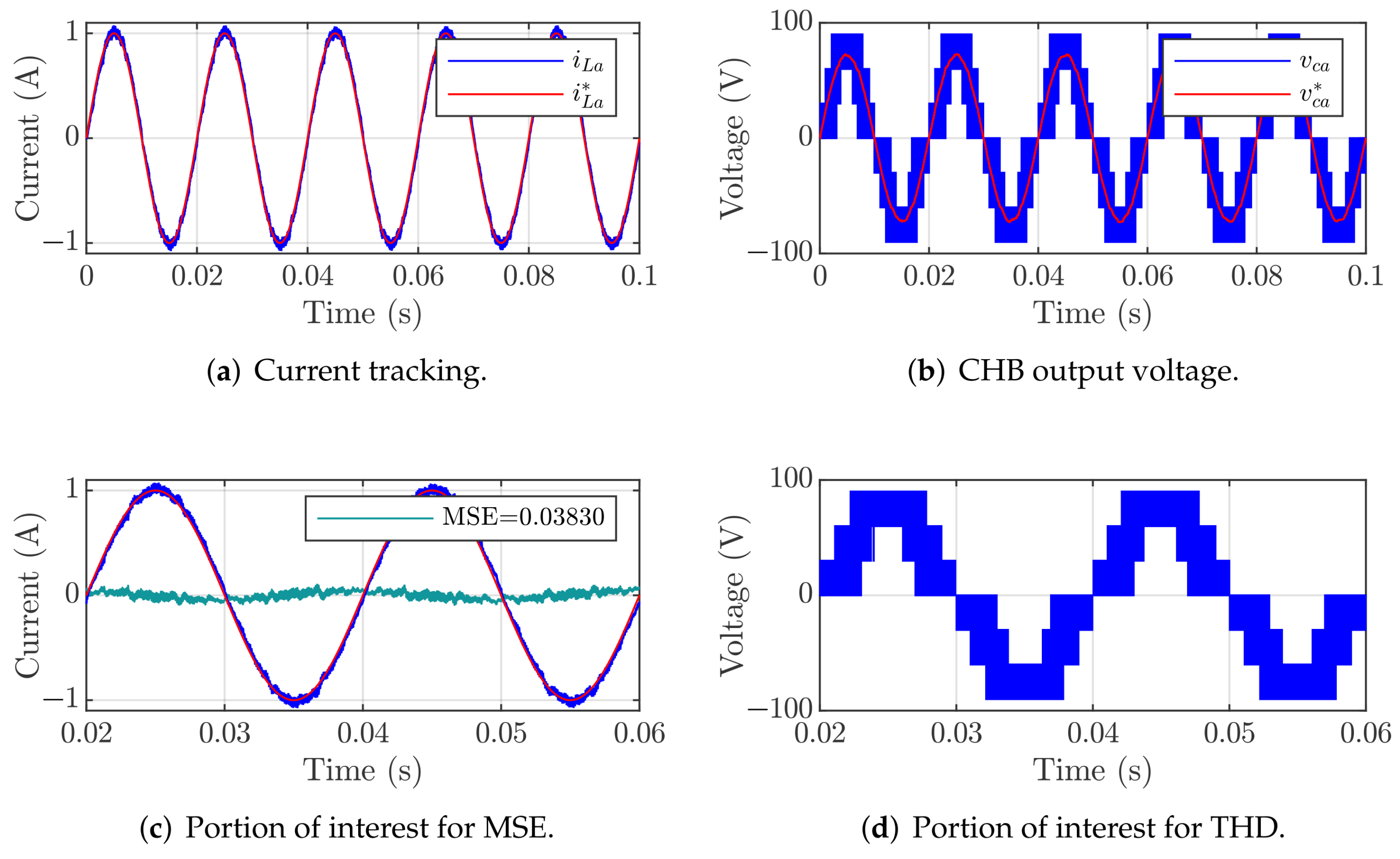
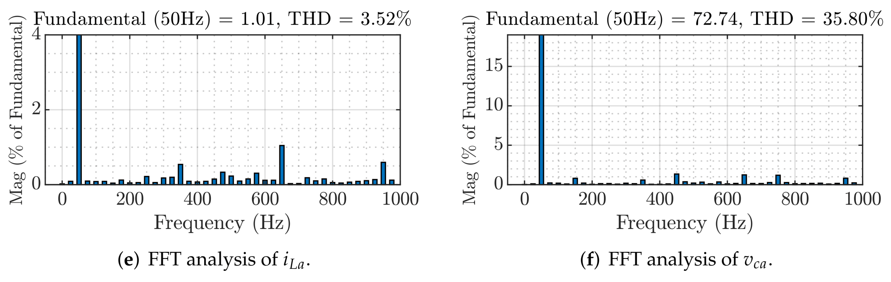
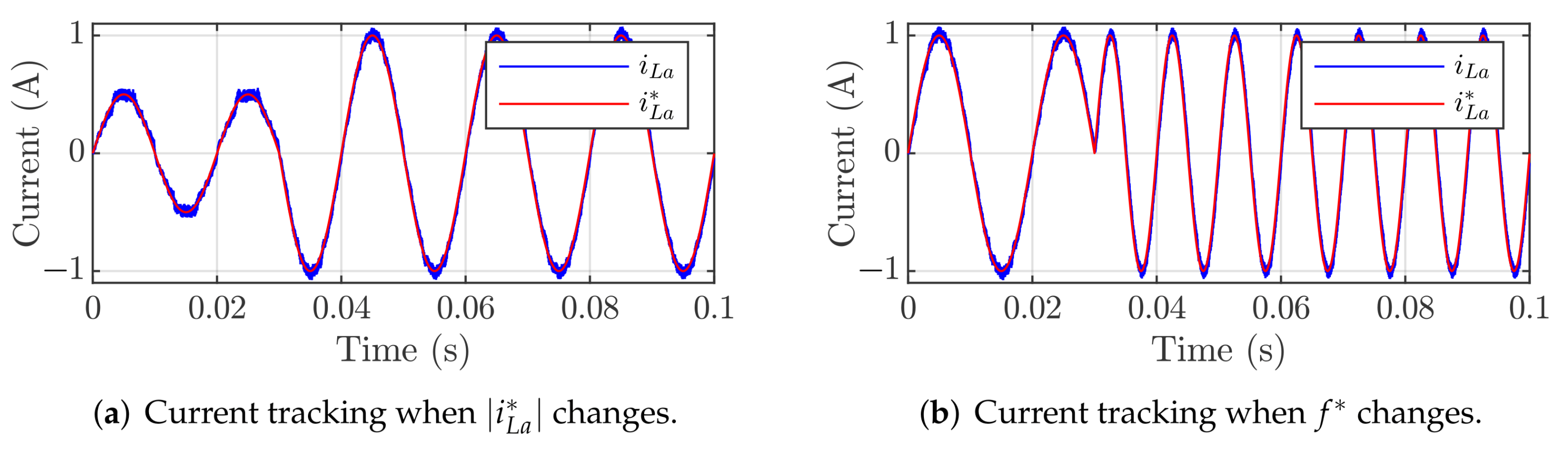
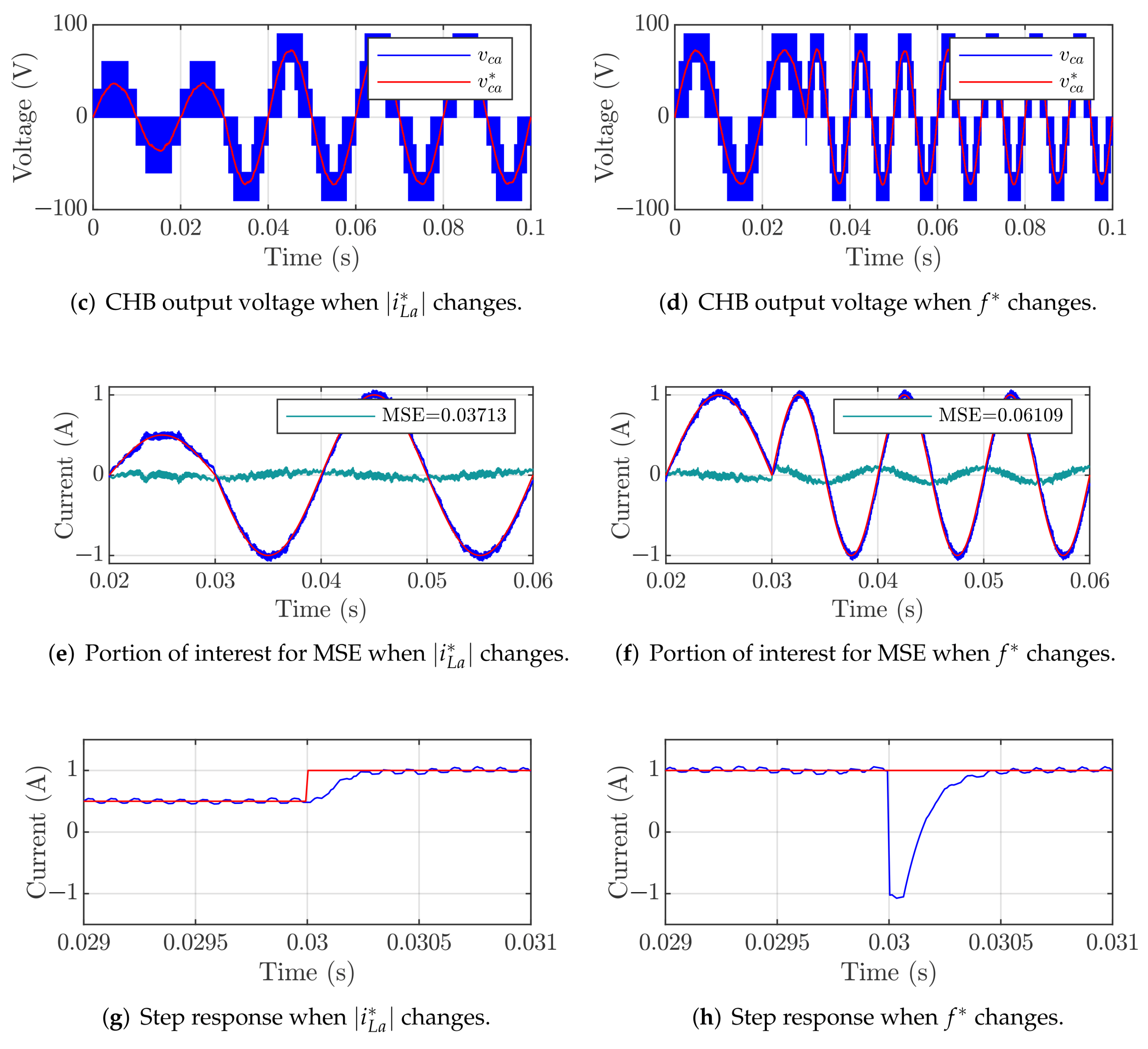
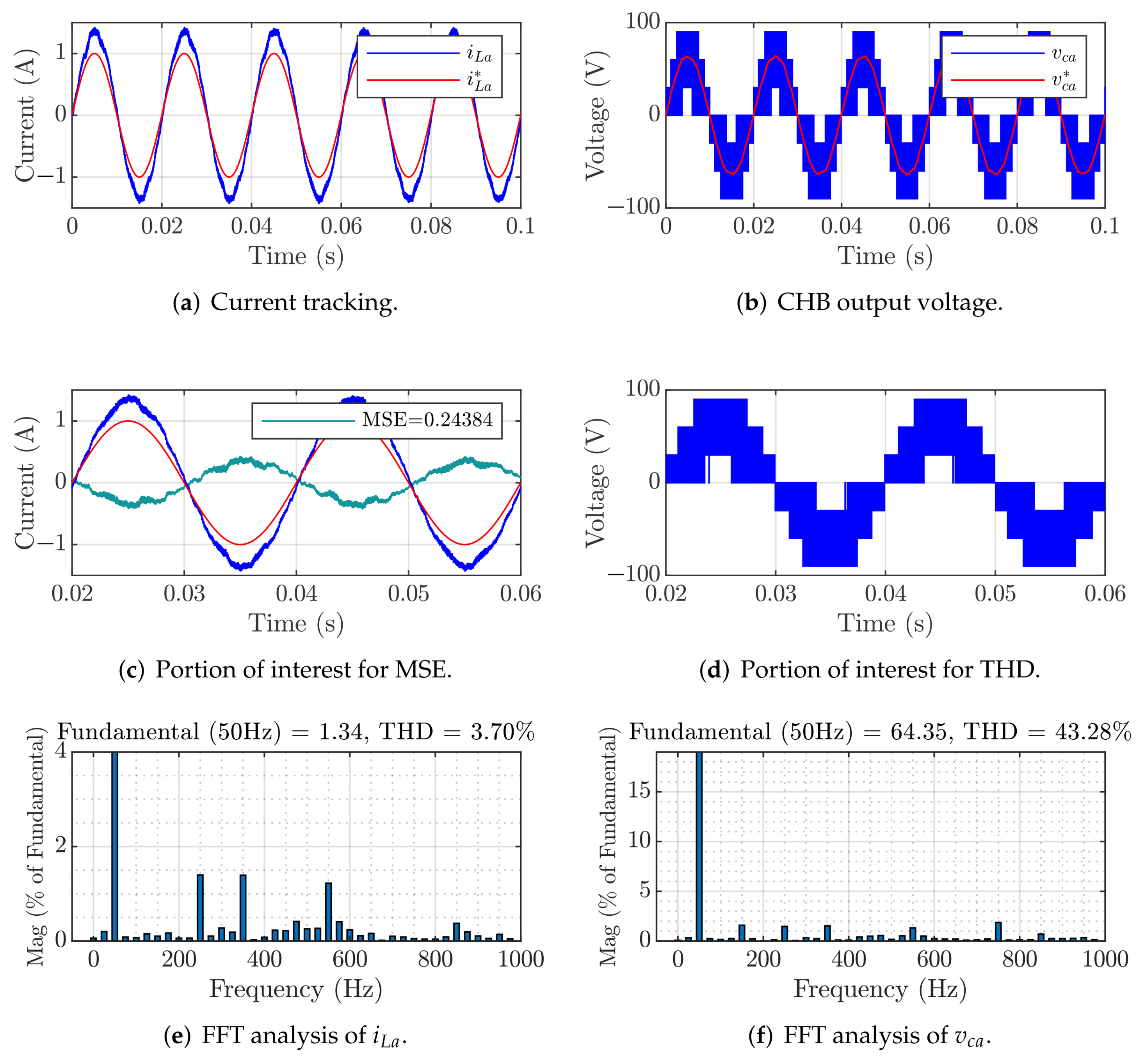
The paper’s primary focus is the implementation of the Discrete-Time Sliding Mode (DTSM) control applied to a seven-level CHB converter, which could present many advantages in comparison to already published current controllers (mainly, its robustness since it offers a tracking error close to zero and a fast dynamic response comparable to that of the MPC). Therefore, simulation and experimental tests have been added to demonstrate the performance of this particular controller. At the same time, the effectiveness of the DTSM is verified under steady-state and transient conditions, respectively, by measuring the mean square error (MSE) and total harmonic distortion (THD).
The manuscript is organized as follows: the topology description and mathematical model of the seven-level CHB are presented in Section 2. In Section 3, the DTSM controller is described. Section 4 shows the simulation and experimental results in steady-state and transient conditions for performance analysis of the DTSM. Section 5 exposes the comparative performance of DTSM with the popular MPC technique. Finally, Section 6 summarizes the conclusion.

2. Topology Description and Mathematical Model

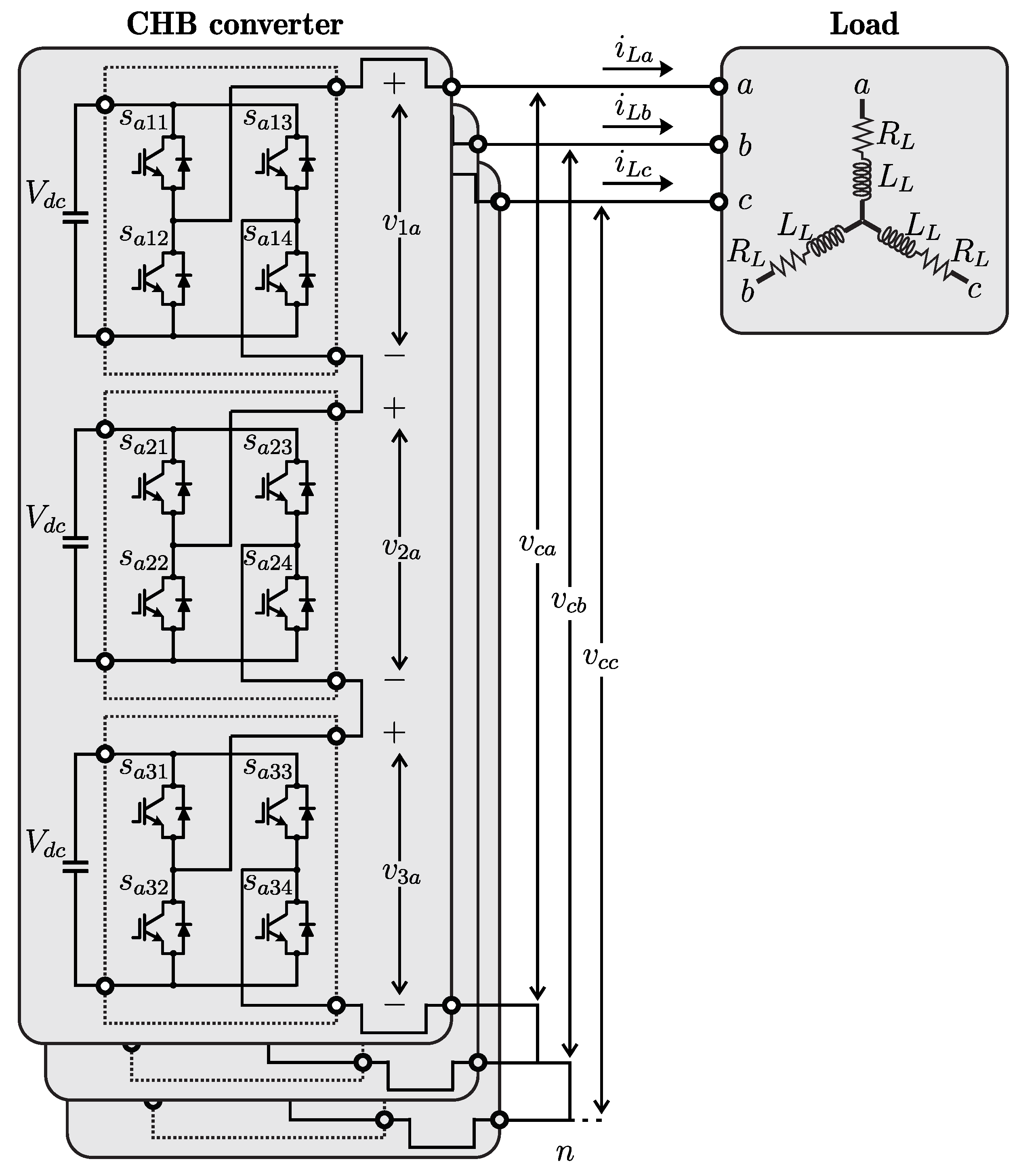
The three-phase seven-level CHB converter is shown in Figure 1. Each leg is composed of 3 identical H-bridge cells, which means that all DC-link voltages have the same values V d c . The output voltage v i ϕ of each cell depends on the states s ϕ i j (0 → open and 1 → closed) of the four switching devices, as described by:
v i ϕ = s ϕ i 1 s ¯ ϕ i 2 s ϕ i 3 s ¯ ϕ i 4 V d c
where i is the corresponding cell 1, 2 or 3, j the corresponding switching device 1, 2, 3 or 4, and ϕ the corresponding phase a, b or c. However, only switches 1 and 3 are used to control one cell since they are always complementary with switches 2 and 4, respectively, to prevent short-circuit on DC-links. In this way, v i ϕ has only three possible values, as shown in Table 1.
The output voltage of the converter v c ϕ can be obtained as the sum of the v i ϕ voltages as follows:
v c ϕ = i = 1 3 v i ϕ
and referring to Table 1, the seven possible values for v c ϕ are: 3 V d c , 2 V d c , V d c , 0, V d c , 2 V d c , and 3 V d c
Considering the R L - L L load fed by the CHB converter as shown in Figure 1, the continuous model (for each phase) of the system is:
v c ϕ = R L i L ϕ + L L d i L ϕ d t
where the load currents are defined by i L ϕ considering that ϕ includes the corresponding phase a, b or c.
From Equation (3), using forward Euler discretization, we obtain:
i L ϕ [ k + 1 ] = 1 R L T s L L i L ϕ [ k ] + T s L L v c ϕ [ k ]
where T s is the sampling time and k identifies the actual discrete-time sample.
If state variables are defined by:
x 1 [ k ] x 2 [ k ] x 3 [ k ] T = i L a [ k ] i L b [ k ] i L c [ k ] T
and the input and output variables by
u 1 [ k ] u 2 [ k ] u 3 [ k ] T = v c a [ k ] v c b [ k ] v c c [ k ] T
y 1 [ k ] y 2 [ k ] y 3 [ k ] T = x 1 [ k ] x 2 [ k ] x 3 [ k ] T
the state-space representation is obtained:
x 1 [ k + 1 ] x 2 [ k + 1 ] x 3 [ k + 1 ] = a 1 0 0 0 a 1 0 0 0 a 1 x 1 [ k ] x 2 [ k ] x 3 [ k ] + b 1 0 0 0 b 1 0 0 0 b 1 u 1 [ k ] u 2 [ k ] u 3 [ k ]
y 1 [ k ] y 2 [ k ] y 3 [ k ] = 1 0 0 0 1 0 0 0 1 x 1 [ k ] x 2 [ k ] x 3 [ k ]
where the coefficients a 1 and b 1 of Equation (8) are defined according to the following equations:
a 1 = 1 R L T s L L
b 1 = T s L L

3. Discrete-Time Sliding Mode Current Control

In this section, the proposed controller, named DTSM, is presented. First, the design procedure is described, and then, a stability analysis is proposed. Last, the convergence time for the system is estimated.

3.1. Design Procedure

The synthesis control procedure consists of the following steps:
  • Define the sliding surface.
  • Satisfy the sliding condition by selecting the reaching law.
For the current tracking problem, the conventional discrete-time sliding surfaces are defined for i = 1 , 2 , 3 as follows:
S i [ k ] = e i [ k ] = x i [ k ] x i [ k ]
where e i [ k ] are the current tracking errors with x i [ k ] as the desired load currents (reference variables are represented through the superscript ).
To satisfy the sliding conditions
S i [ k ] = S i [ k + 1 ] = 0
the reaching law is chosen as:
S i [ k + 1 ] = Λ S i [ k ] L T s sign S i [ k ]
where Λ is chosen between 0 and 1, while L > 0 and the sign is defined by:
sign S i [ k ] = 1 , if S i [ k ] > 0 0 , if S i [ k ] = 0 1 , if S i [ k ] < 0
Then, from Equations (12) and (14), we have:
e i [ k + 1 ] = x i [ k + 1 ] x i [ k + 1 ] = Λ e i [ k ] L T s sign e i [ k ]
Considering Equations (8) and (16) results in:
x i [ k + 1 ] a 1 x i [ k ] b 1 u i [ k ] = Λ e i [ k ] L T s sign e i [ k ]
Then, resolving Equation (17) gives the control law for the load currents as follows:
u i [ k ] = x i [ k + 1 ] a 1 x i [ k ] Λ e i [ k ] + L T s sign e i [ k ] b 1
Figure 2 shows the DTSM control scheme for the CHB converter, where the control actions represented by Equation (18) are normalized between −1 and 1 and sent to a modulator to synthesize the output voltage of the CHB converter. The modulation stage consists of the phase-shift carrier pulse width modulation (PSC-PWM) technique, considering the carrier signal amplitude equal to 1 and the carrier frequency ( f c r ) equal to the sampling frequency.

3.2. Stability Analysis

The existence of a quasi-sliding mode should be discussed to prove the stability of the closed-loop system. In other words, the system is stable if the following conditions hold for i = 1 , 2 , 3 :
e i [ k ] > ε ε e i [ k + 1 ] < e i [ k ] e i [ k ] < ε e i [ k ] < e i ( k + 1 ) ε | e i [ k ] | ε | e i [ k + 1 ] | ε
where ε > 0 depicts the bandwidth of the quasi-sliding mode. In this paper, we choose ε = L T s . A simplified version of Equation (16) gives for i = 1 , 2 , 3 :
e i [ k + 1 ] = Λ e i [ k ] L T s sign ( e i [ k ] )
1.
Assuming that e i [ k ] > L T s means that e i [ k ] > 0 , sign ( e i [ k ] ) = 1 and:
e i [ k + 1 ] = Λ e i [ k ] L T s e i [ k + 1 ] ) e i [ k ] = ( Λ 1 ) e i [ k ] L T s
since ( Λ 1 ) < 0 , then e i [ k + 1 ] e i [ k ] < 0 e i [ k + 1 ] < e i [ k ] .
Furthermore, L T s e i [ k + 1 ] can be written as:
Λ e i [ k ] L T s L T s
Hence,
e i [ k ] 0
which is true with the assumption made.
2.
Now, assuming e i [ k ] < L T s means that e i [ k ] < 0 and sign ( e i [ k ] ) = 1 . Then, e i [ k ] < e i [ k + 1 ] is similar to:
e i [ k ] < Λ e i [ k ] + L T s ( 1 Λ ) e i [ k ] < L T s
which is always true for any positive value of L. In addition, we can rewrite e i [ k + 1 ] < L T s as:
Λ e i [ k ] + L T s < L T s
which is true since e i [ k ] < 0 . Finally, the second condition of Equation (19) holds.
3.
Now, let us assume that | e i [ k ] | L T s , then:
a.
If e i [ k ] > 0 , then | e i ( k ) | L T s becomes:
0 < e i [ k ] < L T s
Multiplying Equation (26) by Λ and adding L T s to all the parts leads to:
L T s < e i [ k + 1 ] < ( Λ 1 ) L T s < L T s | e i [ k + 1 ] | L T s
b.
If e i [ k ] < 0 , then | e i [ k ] | L T s becomes:
L T s < e i [ k ] < 0
Again, by multiplying Equation (28) with Λ and adding L T s to all the parts gives:
L T s < ( 1 Λ ) L T s < e i [ k + 1 ] < L T s | e i [ k + 1 ] | < ε
Hence,
| e i [ k + 1 ] | < ε = L T s
This implies that the third condition of Equation (19) is always true.
As a result, the conditions in Equation (19) are met, which proves the occurrence of a convergent quasi-sliding mode. Thus, the proposed DTSM is stable.

3.3. Convergence Time

Let us suppose that e i [ 0 ] 0 and sign ( e i [ 0 ] ) = sign ( e i [ 1 ] ) = = sign ( e i [ k i + 1 ] ) .
1.
Firstly, assuming that e i [ 0 ] > 0 and e i [ m ] > 0 for all m ( k i + 1 ) leads to:
e i [ 1 ] = Λ e i [ 0 ] L T s e i [ 0 ] L T s e i [ 2 ] e i [ 1 ] L T s e i [ 0 ] 2 L T s e i [ m ] e i [ m 1 ] L T s e i [ 0 ] m L T s | e i [ 0 ] | m L T s
Hence, it is obvious that there exists a step k i = | e i [ 0 ] | L T s that ensures
| e i [ 0 ] | k i L T s = 0
It follows that
e i [ k i + 1 ] | e i [ 0 ] | ( k i + 1 ) L T s < | e i [ 0 ] | k i L T s = 0
which is contradictory to the fact that e i [ m ] > 0 , m ( k i + 1 ) .
2.
Firstly, assuming that e i [ 0 ] < 0 and e i [ m ] < 0 for all m ( k i + 1 ) leads to:
e i [ 1 ] = Λ e i [ 0 ] + L T s e i [ 0 ] + L T s e i [ 2 ] e i [ 1 ] + L T s e i [ 0 ] + 2 L T s e i [ m ] e i [ m 1 ] + L T s e i [ 0 ] + m L T s | e i [ 0 ] | + m L T s
Thus, it is obvious that k i = | e i [ 0 ] | L T s verifies
| e i [ 0 ] | + k i L T s = 0
It follows that
e i [ k i + 1 ] | e i [ 0 ] | + ( k i + 1 ) L T s > | e i [ 0 ] | + k i L T s = 0
which is contradictory to the fact that e i [ m ] < 0 , m ( k i + 1 ) .
This concludes that each current will reach its desired reference within at most k i + 1 steps, where for i = 1 , 2 , 3 :
k i = | e i [ 0 ] | L T s

4. Simulation and Experimental Results

The performance of the DTSM controller is analyzed in steady-state and transient conditions. For steady-state conditions, the DTSM technique behavior is studied using a reference amplitude i L ϕ = 1 A and a reference frequency f = 50 Hz. For transient conditions, the analysis is performed as follows. On the one hand, after a change in the reference amplitude from 0.5 A to 1 A (with a constant reference frequency equal to 50 Hz). In addition, on the other hand, after a change in the reference frequency, from 50 Hz to 100 Hz (with constant reference amplitude and equal to 1 A). Simulation and experimental results are analyzed in terms of MSE obtained between reference and measured load currents and THD of the CHB output voltages and load currents. MSE is measured in amperes (A) and obtained as follows:
MSE i L ϕ = 1 N j = 1 N i L ϕ i L ϕ 2
where N is the number of samples. While THD is obtained as follows:
THD Ψ ϕ = 1 Ψ ϕ 1 2 i = 2 N Ψ ϕ i 2
where Ψ ϕ 1 corresponds to the fundamental variable (voltage or current) whereas Ψ ϕ i is the harmonic variable (multiple of the fundamental variable).

4.1. Simulation Results

Numerical integration based on first-order Euler’s algorithm has been computed to the progress of the proposed controller. MATLAB/Simulink R2018b simulations have been performed in order to verify the feasibility of the DTSM control law given by Equation (18), considering the simulation parameters listed in Table 2.
Figure 3 shows simulation results for phase a in steady-state condition. Figure 3a shows the time-evolution of the load current i L a and current reference i L a . Figure 3b presents the control action u 1 = v c a and CHB output voltage v c a . Figure 3c,d denotes a portion of samples (two cycles) used for the computation of the MSE and THD parameters. Hence, N = 5860 in Equations (38) and (39). Figure 3c also illustrates the dynamic behavior of the current tracking error with an MSE value of 0.03829 A. Figure 3e presents the fast Fourier transform analysis of the load current i L a with a THD value of 3.52%. At the same time, Figure 3f presents the fast Fourier transform analysis of the CHB output voltage v c a with a THD value of 35.80%. Similar simulation results in steady-state condition were obtained for phases b and c, and Table 3 summarizes the values obtained for THD and MSE parameters.
Figure 4 shows simulation results for phase a in transient conditions. Figure 4a shows the transient response of the load current i L a when a sudden change in the amplitude reference from 0.5 A to 1 A at t = 0.03 s is applied. Figure 4c demonstrates the control action u 1 = v c a value and CHB output voltage v c a variation when the reference amplitude current changes. Figure 4b also presents the transient response of the load current i L a , for the case of a sudden change in the reference frequency from 50 Hz to 100 Hz at t = 0.03 s. Figure 4d demonstrates the control action u 1 = v c a value and the CHB output voltage v c a variation when the reference frequency changes. Figure 4e,f denotes a portion of samples (two cycles) used for the computation of the MSE parameter. Hence, N = 5860 in Equation (38). The current tracking error behavior for both cases is illustrated in Figure 4e (MSE value of 0.03713 A) and Figure 4f (MSE value of 0.06109 A). Similar simulation results in transient conditions were obtained for phases b and c. To quantify the dynamic response, the results in a b c frame are converted into the d q 0 frame using Park’s transformation (invariant amplitude). Figure 4g illustrates the case for current i L d when i L d = i L a changes and Figure 4h when f changes; they present a rise time of 0.3 and 0.4 ms, respectively. In both cases, an overshoot of less than 1% is observed.
Figure 5 shows the simulation results for phase a in the presence of parametric uncertainties, varying the value of the load ( R L equal to 48.13 Ω ) and keeping the reference amplitude at 1 A and the reference frequency at 50 Hz. The value of R L has also been maintained equal to 72.2 Ω in Equation (18). Figure 5a shows the time-evolution of the load current i L a and current reference i L a . Figure 5b presents the control action u 1 = v c a and CHB output voltage v c a . Figure 5c,d denotes a portion of samples (two cycles) used for the computation of the MSE and THD parameters. Hence, N = 5860 in Equations (38) and (39). Figure 3c also illustrates the dynamic behavior of the current tracking error with an MSE value of 0.24383 A. Figure 5e presents the fast Fourier transform analysis of the load current i L a with a THD value of 3.70%. At the same time, Figure 5f presents the fast Fourier transform analysis of the CHB output voltage v c a with a THD value of 43.28%. Similar simulation results in steady-state condition were obtained for phases b and c, and Table 4 summarizes the values obtained for THD and MSE parameters.

4.2. Experimental Results

For the experimental tests of the DTSM control described in Section 3, the test equipment, shown in Figure 6, is examined to validate its effectiveness, employing an AC variable load bank as R L (it can vary from 1 kW to 20 kW). The other electrical and control parameters are the same as described in Table 2. The seven-level CHB converter is based on CAS120M12BM2 series SiC-MOSFET half-bridge modules, and nine independent voltage DC sources. A dSPACE MicroLabBox DS1201 control unit and Simulink version 9.5 have been used to implement the DTSM control technique. RTI FPGA programming block-set version 3.9.3 and Vivado 2019.2 have been used to implement the digital modulator on the dSPACE FPGA platform. Normalization is done between −128 and +127, because the carrier signals (sawtooth) are formed from signed 8-bit digital counters. On the other hand, the SiC-MOSFET half-bridge modules have a turn-on delay time of t o n = 38 ns and a turn-off delay time of t o f f = 70 ns; therefore, as established in [50], a dead time period of 1 μ s is taken. Furthermore, considering a maximum switching frequency of semiconductor devices of 100 kHz, the changes in the states of s ϕ i j (from 0 to 1, or from 1 to 0) must occur in at least 11 μ s.
The choice of an n-bits counter and a sampling period of T s   μ s establishes a step of T s / 2 n   μ s for each counter, i.e., the carrier signal must fit exactly in one sampling period of the controller. Another requirement is that T s / 2 n   μ s must be a multiple of the FPGA clock (10 ns). With the choice of T s = 102.4 μ s, a step of 0.4 μ s results for each counter. Current sensors of the CS60-100L series have been used for the experimental measurements. Finally, the acquired results through the Tektronix TDS3034C series digital oscilloscope are analyzed through MATLAB/Simulink R2018b code.
Figure 7 and Figure 8 show the experimental results for phase a in steady-state condition and a load of 2 kW as R L . Figure 7a shows the screenshot of the oscilloscope with the voltage and current in phase a and Figure 7b the three-phase currents. Figure 8a,b denotes a portion of samples (two cycles) used for the computation of the MSE and THD parameters. Hence, N = 6000 in Equations (38) and (39). Figure 8a also illustrates the dynamic behavior of the current tracking error with an MSE value of 0.17022 A. Figure 8c presents the fast Fourier transform analysis of the load current i L a with a THD value of 24.34%. At the same time, Figure 8d presents the fast Fourier transform analysis of the CHB output voltage v c a with a THD value of 77.14%. Similar simulation results in steady-state conditions were obtained for phases b and c, and Table 5 summarizes the values obtained for THD and MSE parameters.
Figure 9 and Figure 10 show the experimental results for phase a in transient state conditions. Figure 9a shows the transient response of the load current i L a and the CHB output voltage v c a when a sudden change in the amplitude reference from 0.5 A to 1 A is applied. Figure 9b also presents the transient response of the load current i L a and the CHB output voltage v c a , for the case of a sudden change in the reference frequency, from 50 Hz to 100 Hz. Figure 10a,b denotes a portion of samples (two cycles) used for the computation of the MSE parameter. Hence, N = 6000 in Equation (38). The current tracking error behavior for both cases is illustrated in Figure 10a (MSE value of 0.19473 A) and Figure 10b (MSE value of 0.18343 A). Similar experimental results in transient conditions were obtained for phases b and c, showing a fast dynamic response during the transient.
Figure 11 and Figure 12 show the experimental results for phase a in the presence of parametric uncertainties. Experimental tests were carried out by varying the load value (3 kW as R L ) and keeping the reference amplitude at 1 A and the reference frequency at 50 Hz. Figure 11a shows the screenshot of the oscilloscope with the voltage and current in phase a and Figure 11b the three-phase currents. Figure 12a,b denotes a portion of samples (two cycles) used for the computation of the MSE and THD parameters. Hence, N = 6000 in Equations (38) and (39). Figure 12a also illustrates the dynamic behavior of the current tracking error with an MSE value of 0.19080 A. Figure 12c presents the fast Fourier transform analysis of the load current i L a with a THD value of 29.44%. At the same time, Figure 12d presents the fast Fourier transform analysis of the CHB output voltage v c a with a THD value of 103.63%. Similar simulation results in steady-state conditions were obtained for phases b and c, and Table 6 summarizes the values obtained for THD and MSE parameters.

5. Comparison between DTSM and FCS-MPC

For comparative purposes, simulation and experimental tests have also been added for the finite-control-set model predictive control (FCS-MPC) in combination with a modulation scheme based on PSC-PWM. This paper does not describe the design procedure for this technique, because the authors have a plan to make a detailed comparative analysis in another paper, meanwhile, interested readers may refer to [51]. First, simulation tests have been added for proportional-integral (PI) control and FCS-MPC, both with PSC-PWM. The PI control law for the load currents are:
u i [ k ] = K p e i [ k ] + T s K i j = 0 k e i [ k ]
with K p = 21 and K i = 100,000, which have been obtained heuristically based on the trial and error method. The tests are carried out using the same scheme of Figure 2, replacing the DTSM controller with PI or FCS-MPC and considering the simulation parameters listed in Table 2. Table 7 and Table 8 summarize the values obtained from the simulations for the THD and MSE parameters for PI control, and Table 9 and Table 10 summarize the values obtained from the simulations for the THD and MSE parameters for FCS-MPC. These results show a better performance in the current tracking of the FCS-MPC compared with PI, from the point of view of the MSE parameter. Table 11 and Table 12 summarize the values obtained from the experimental tests for FCS-MPC.

6. Conclusions

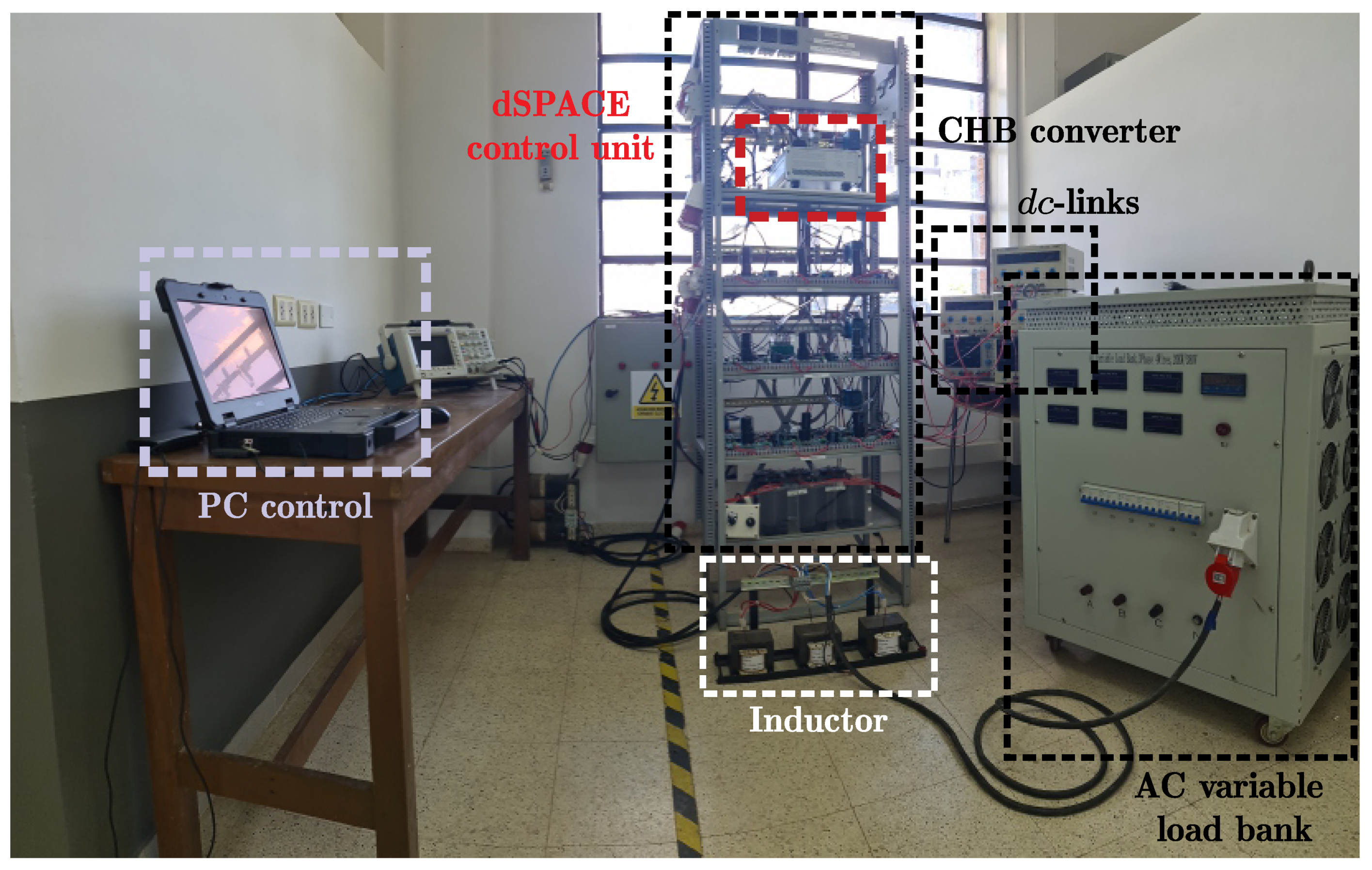
A real-time implementation of a discrete-time sliding mode control in combination with a modulation scheme based on phase-shifted carrier modulation was applied to a seven-level CHB converter based on SiC-MOSFET half-bridge modules.
Steady-state simulation results show that DTSM control has a 39% reduction in MSE of current tracking (0.03837 A vs. 0.06293 A on average) and a 51% reduction in THD of the load current (3.54% vs. 7.34% on average), compared to FCS-MPC. Transient-state simulation results show that DTSM control has a 9% reduction in MSE of current tracking (0.09702 A vs. 0.10645 A on average) and a similar rise-time (between 0.3 and 0.4 ms), compared to FCS-MPC.
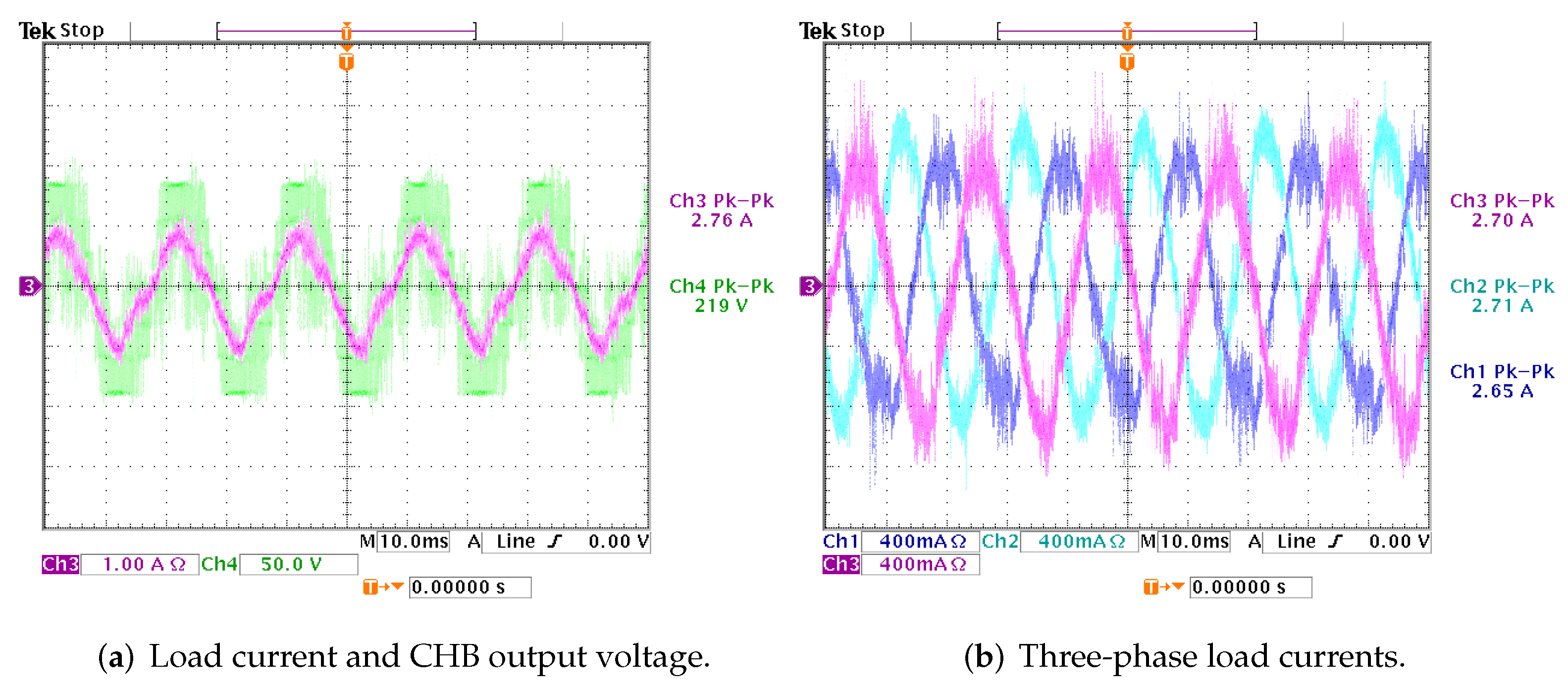
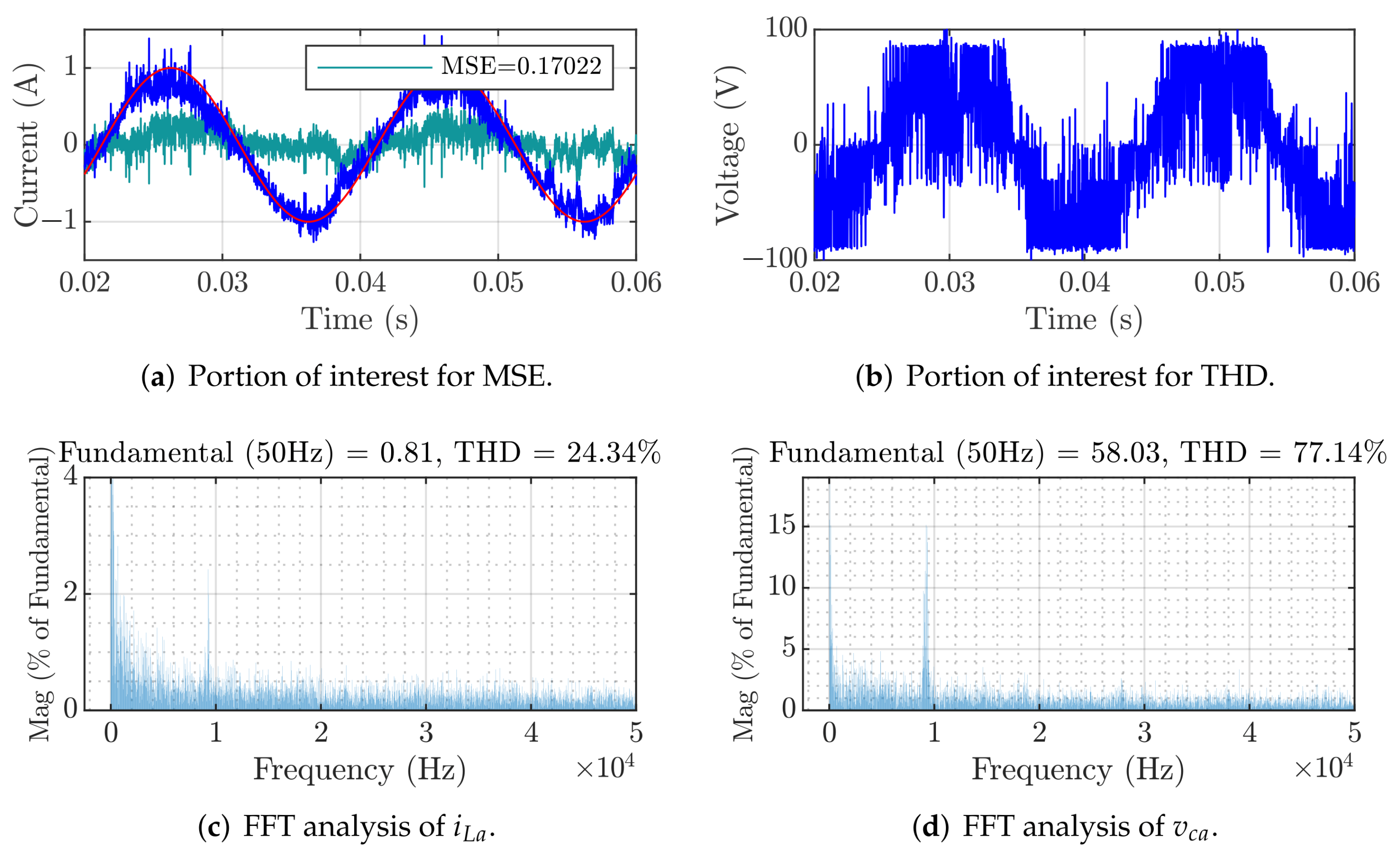
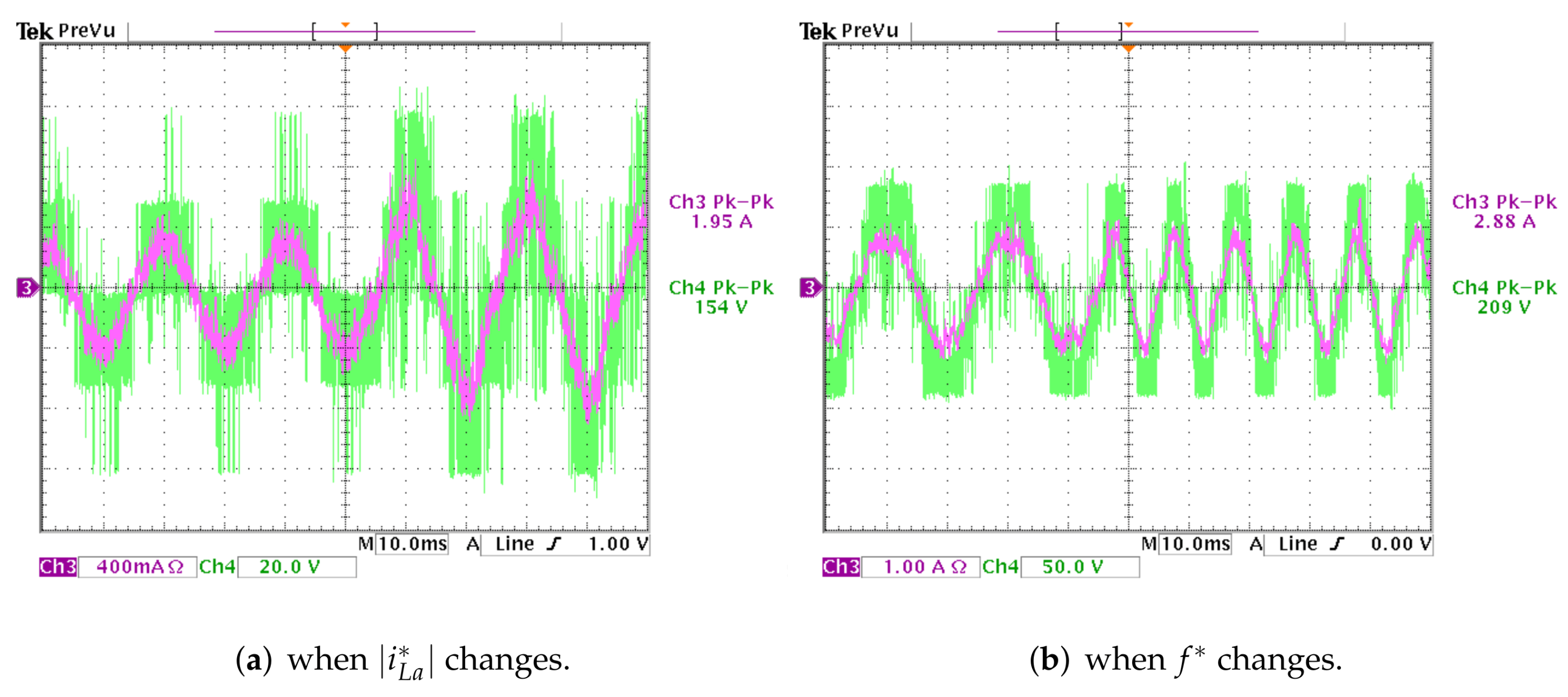
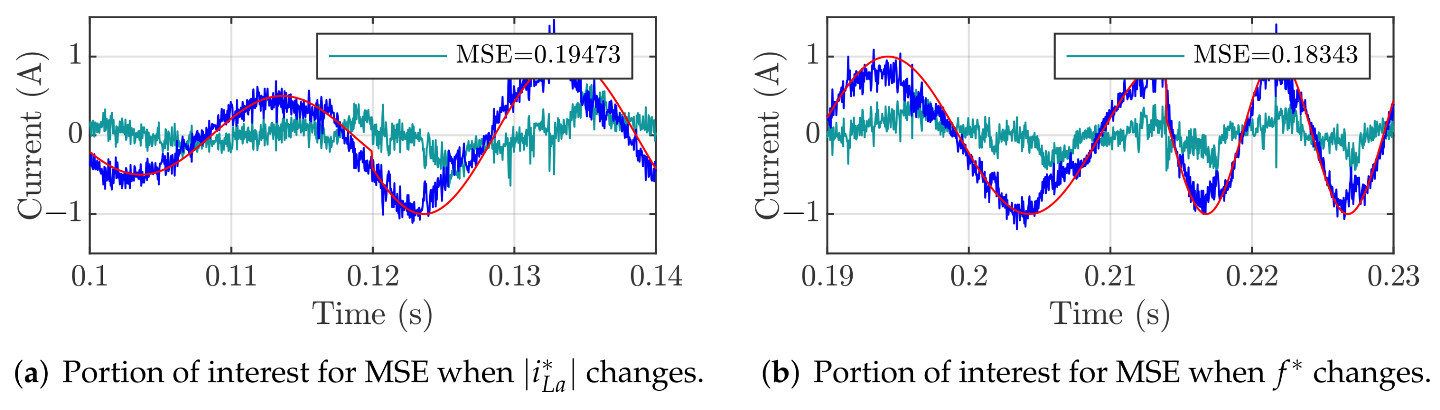
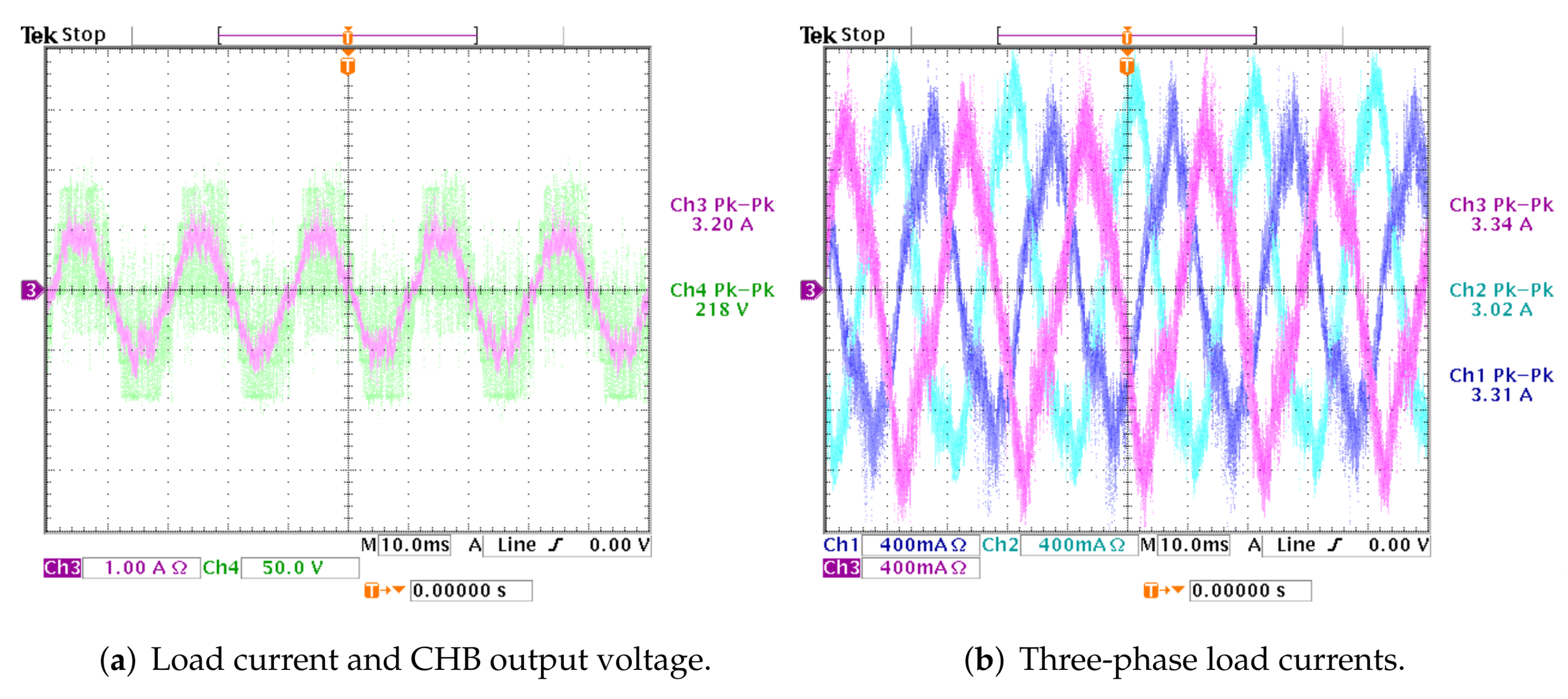
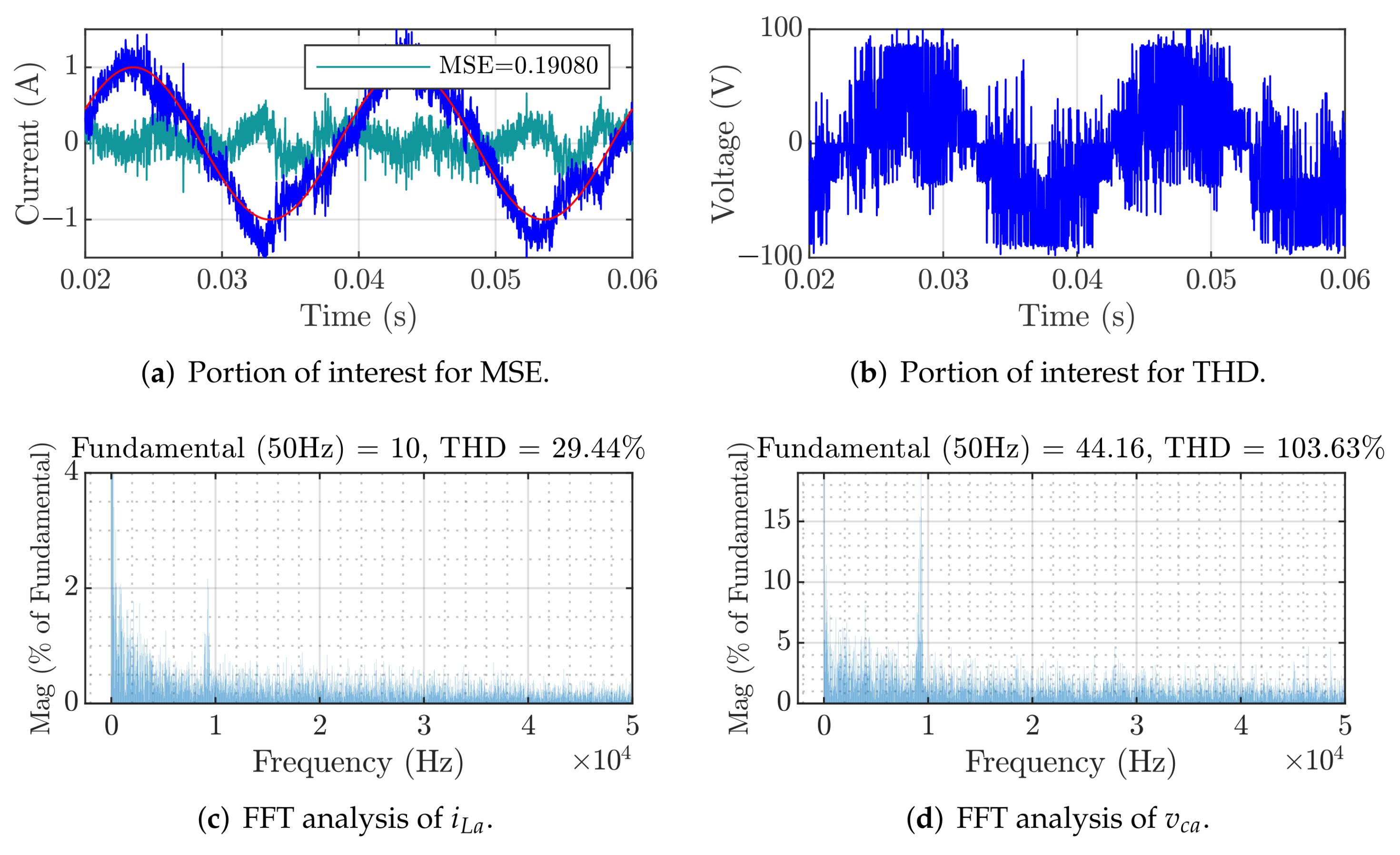
Steady-state experimental results show that DTSM control has a 22% reduction in MSE of current tracking (0.17053 A vs. 0.22066 A on average) and a slight 1% reduction in THD of the load current (24.62% vs. 24.87% on average), compared to FCS-MPC. Transient-state experimental results show that DTSM control has a 12% reduction in MSE of current tracking (0.19761 A vs. 0.22461 A on average) and a similar rise-time (between 0.4 and 0.5 ms), compared to FCS-MPC.
From the point of view of robustness, simulation and experimental results show that DTSM control is insensitive to load parameter variations in terms of THD of the load current, compared to steady-state results (simulation: 3.71% vs. 3.54%, experimental: 24.62% vs. 20.49% on average). In addition, in terms of MSE of current tracking, experimental results confirm that the proposed controller is robust against load parameter variations (experimental: 0.14655 A vs. 0.17053 A on average). In the robustness test, a slight increase in the THD of the output voltage is observed due to the need to synthesize a low voltage to maintain the same reference current amplitude.
The differences between simulations and experimental results are mainly due to the non-modeling of the circuits that involve the signal conditioners (digital and analog), snubbers, the switching devices, as well as the electrical noises (internal and external), and the delays associated with the digital implementation.

Author Contributions

Conceptualization, L.C., Y.K., J.P., A.R., J.R. and R.G.; methodology, L.C. and J.P. software, L.C. and J.P.; validation, L.C., J.P. and A.R.; formal analysis, L.C., Y.K., J.P., A.R., J.R. and R.G.; investigation, L.C., J.P., A.R.,Y.K., M.A., J.R. and R.G.; resources, L.C., J.P., A.R., M.A., J.R. and R.G.; data curation, L.C., J.P., A.R., J.R. and R.G.; writing, original draft preparation, L.C. and M.A.; writing, review and editing, L.C., M.A. and J.R.; visualization, L.C. and J.P.; project administration, R.G., and J.R.; funding acquisition, R.G. and J.R. All authors have read and agreed to the published version of the manuscript.

Funding

This research has been funded through the Consejo Nacional de Ciencia y Tecnología (CONACYT)-Paraguay, Grant Number POSG16-05.

Conflicts of Interest

The authors declare no conflict of interest.

Abbreviations

The abbreviations used in this document are listed below:
CHBCascade H-bridge
DTSMDiscrete-time sliding mode
FCFlying capacitor
FCS-MPCFinite-control-set MPC
MPCModel predictive control
MSEMean square error
NPCNeutral-point clamped
PSC-PWMPhase-shift carrier pulse width modulation
SMCSliding mode control
THDTotal harmonic distortion

References

  1. Bhagwat, P.M.; Stefanovic, V.R. Generalized Structure of a Multilevel PWM Inverter. IEEE Trans. Ind. Appl. 1983, IA-19, 1057–1069. [Google Scholar] [CrossRef]
  2. Mhiesan, H.; Umuhoza, J.; Mordi, K.; Farnell, C.; Mantooth, H.A. Evaluation of 1.2 kV SiC MOSFETs in multilevel cascaded H-bridge three-phase inverter for medium-voltage grid applications. Chin. J. Electr. Eng. 2019, 5, 1–13. [Google Scholar] [CrossRef]
  3. Carrara, G.; Gardella, S.; Marchesoni, M.; Salutari, R.; Sciutto, G. A new multilevel PWM method: A theoretical analysis. IEEE Trans. Power Electron. 1992, 7, 497–505. [Google Scholar] [CrossRef]
  4. Tolbert, L.M.; Peng, F.Z.; Habetler, T.G. Multilevel converters for large electric drives. IEEE Trans. Ind. Appl. 1999, 35, 36–44. [Google Scholar] [CrossRef] [Green Version]
  5. Tolbert, L.M.; Peng, F.Z.; Habetler, T.G. Multilevel PWM methods at low modulation indices. IEEE Trans. Power Electron. 2000, 15, 719–725. [Google Scholar] [CrossRef]
  6. Nabae, A.; Takahashi, I.; Akagi, H. A New Neutral-Point-Clamped PWM Inverter. IEEE Trans. Ind. Appl. 1981, IA-17, 518–523. [Google Scholar] [CrossRef]
  7. Jayakumar, V.; Chokkalingam, B.; Munda, J.L. A Comprehensive Review on Space Vector Modulation Techniques for Neutral Point Clamped Multi-Level Inverters. IEEE Access 2021, 9, 112104–112144. [Google Scholar] [CrossRef]
  8. Huang, J.; Corzine, K.A. Extended operation of flying capacitor multilevel inverters. IEEE Trans. Power Electron. 2006, 21, 140–147. [Google Scholar] [CrossRef]
  9. Kampitsis, G.; Batzelis, E.I.; Mitcheson, P.D.; Pal, B.C. A Clamping-Circuit-Based Voltage Measurement System for High-Frequency Flying Capacitor Multilevel Inverters. IEEE Trans. Power Electron. 2022, 37, 12301–12315. [Google Scholar] [CrossRef]
  10. Rodriguez, J.; Bernet, S.; Wu, B.; Pontt, J.O.; Kouro, S. Multilevel Voltage-Source-Converter Topologies for Industrial Medium-Voltage Drives. IEEE Trans. Ind. Electron. 2007, 54, 2930–2945. [Google Scholar] [CrossRef]
  11. Celanovic, N.; Boroyevich, D. A comprehensive study of neutral-point voltage balancing problem in three-level neutral-point-clamped voltage source PWM inverters. IEEE Trans. Power Electron. 2000, 15, 242–249. [Google Scholar] [CrossRef]
  12. Hussan, M.R.; Sarwar, A.; Siddique, M.D.; Mekhilef, S.; Ahmad, S.; Sharaf, M.; Zaindin, M.; Firdausi, M. A Novel Switched-Capacitor Multilevel Inverter Topology for Energy Storage and Smart Grid Applications. Electronics 2020, 9, 1703. [Google Scholar] [CrossRef]
  13. Kumari, M.; Siddique, M.D.; Sarwar, A.; Tariq, M.; Mekhilef, S.; Iqbal, A. Recent trends and review on switched-capacitor-based single-stage boost multilevel inverter. Int. Trans. Electr. Energy Syst. 2021, 31, e12730. [Google Scholar] [CrossRef]
  14. Lai, J.S.; Peng, F.Z. Multilevel converters-a new breed of power converters. IEEE Trans. Ind. Appl. 1996, 32, 509–517. [Google Scholar] [CrossRef]
  15. Teodorescu, R.; Blaabjerg, F.; Pedersen, J.K.; Cengelci, E.; Enjeti, P.N. Multilevel inverter by cascading industrial VSI. IEEE Trans. Ind. Electron. 2002, 49, 832–838. [Google Scholar] [CrossRef]
  16. Galván, L.; Gómez, P.J.; Galván, E.; Carrasco, J.M. Optimization-Based Capacitor Balancing Method with Selective DC Current Ripple Reduction for CHB Converters. Energies 2022, 15, 243. [Google Scholar] [CrossRef]
  17. Rodriguez, J.; Franquelo, L.G.; Kouro, S.; Leon, J.I.; Portillo, R.C.; Prats, M.Á.M.; Perez, M.A. Multilevel Converters: An Enabling Technology for High-Power Applications. Proc. IEEE 2009, 97, 1786–1817. [Google Scholar] [CrossRef] [Green Version]
  18. Chan, R.; Kwak, S. Improved Finite-Control-Set Model Predictive Control for Cascaded H-Bridge Inverters. Energies 2018, 11, 355. [Google Scholar] [CrossRef] [Green Version]
  19. Hasan, N.S.; Rosmin, N.; Osman, D.A.A.; Musta’amal@Jamal, A.H. Reviews on multilevel converter and modulation techniques. Renew. Sustain. Energy Rev. 2017, 80, 163–174. [Google Scholar] [CrossRef]
  20. Haw, L.K.; Dahidah, M.S.A.; Almurib, H.A.F. A New Reactive Current Reference Algorithm for the STATCOM System Based on Cascaded Multilevel Inverters. IEEE Trans. Power Electron. 2015, 30, 3577–3588. [Google Scholar] [CrossRef]
  21. Sajadi, R.; Iman-Eini, H.; Bakhshizadeh, M.K.; Neyshabouri, Y.; Farhangi, S. Selective Harmonic Elimination Technique With Control of Capacitive DC-Link Voltages in an Asymmetric Cascaded H-Bridge Inverter for STATCOM Application. IEEE Trans. Ind. Electron. 2018, 65, 8788–8796. [Google Scholar] [CrossRef] [Green Version]
  22. Chang, W.N.; Liao, C.H. Design and Implementation of a STATCOM Based on a Multilevel FHB Converter with Delta-Connected Configuration for Unbalanced Load Compensation. Energies 2017, 10, 921. [Google Scholar] [CrossRef] [Green Version]
  23. Farivar, G.; Hredzak, B.; Agelidis, V.G. Decoupled Control System for Cascaded H-Bridge Multilevel Converter Based STATCOM. IEEE Trans. Ind. Electron. 2016, 63, 322–331. [Google Scholar] [CrossRef]
  24. Xu, C.; Chen, J.; Dai, K. Carrier-Phase-Shifted Rotation Pulse-Width-Modulation Scheme for Dynamic Active Power Balance of Modules in Cascaded H-Bridge STATCOMs. Energies 2020, 13, 1052. [Google Scholar] [CrossRef] [Green Version]
  25. Jung, J.; Lee, J.; Sul, S.; Son, G.T.; Chung, Y. DC Capacitor Voltage Balancing Control for Delta-Connected Cascaded H-Bridge STATCOM Considering Unbalanced Grid and Load Conditions. IEEE Trans. Power Electron. 2018, 33, 4726–4735. [Google Scholar] [CrossRef]
  26. Orcajo, G.A.A.; Diez, J.R.; Cano, J.M.; Norniella, J.G.; González, J.F.P.; Rojas, C.H.; Ardura, P.; Cifrián, D. Enhancement of Power Quality in an Actual Hot Rolling Mill Plant Through a STATCOM. IEEE Trans. Ind. Appl. 2020, 56, 3238–3249. [Google Scholar] [CrossRef]
  27. Baidya, R.; Aguilera, R.P.; Acuña, P.; Vazquez, S.; Mouton, H.d.T. Multistep Model Predictive Control for Cascaded H-Bridge Inverters: Formulation and Analysis. IEEE Trans. Power Electron. 2018, 33, 876–886. [Google Scholar] [CrossRef] [Green Version]
  28. He, T.; Wu, M.; Lu, D.D.C.; Song, K.; Zhu, J. Model Predictive Sliding Control for Cascaded H-Bridge Multilevel Converters With Dynamic Current Reference Tracking. IEEE J. Emerg. Sel. Top. Power Electron. 2022, 10, 1409–1421. [Google Scholar] [CrossRef]
  29. Kouro, S.; Perez, M.A.; Rodriguez, J.; Llor, A.M.; Young, H.A. Model Predictive Control: MPC’s Role in the Evolution of Power Electronics. IEEE Ind. Electron. Mag. 2015, 9, 8–21. [Google Scholar] [CrossRef]
  30. Gregor, R.; Pacher, J.; Renault, A.; Comparatore, L.; Rodas, J. Model Predictive Control of a Modular 7-Level Converter Based on SiC-MOSFET Devices—An Experimental Assessment. Energies 2022, 15, 5242. [Google Scholar] [CrossRef]
  31. Utkin, V.I. Sliding mode control design principles and applications to electric drives. IEEE Trans. Ind. Electron. 1993, 40, 23–36. [Google Scholar] [CrossRef] [Green Version]
  32. Tan, S.C.; Lai, Y.M.; Tse, C.K. A unified approach to the design of PWM-based sliding-mode voltage controllers for basic DC-DC converters in continuous conduction mode. IEEE Trans. Circuits Syst. I Regul. Pap. 2006, 53, 1816–1827. [Google Scholar] [CrossRef] [Green Version]
  33. Gonzalez Montoya, D.; Ortiz, P.; Ramos-Paja, C. Fixed-frequency implementation of sliding-mode controllers for photovoltaic systems. Int. J. Energy Environ. Eng. 2019, 10, 287–305. [Google Scholar] [CrossRef] [Green Version]
  34. Flores-Bahamonde, F.; Valderrama-Blavi, H.; Bosque-Moncusi, J.M.; García, G.; Martínez-Salamero, L. Using the sliding-mode control approach for analysis and design of the boost inverter. IET Power Electron. 2016, 9, 1625–1634. [Google Scholar] [CrossRef]
  35. Abeywardana, D.B.W.; Hredzak, B.; Agelidis, V.G. A Fixed-Frequency Sliding Mode Controller for a Boost-Inverter-Based Battery-Supercapacitor Hybrid Energy Storage System. IEEE Trans. Power Electron. 2017, 32, 668–680. [Google Scholar] [CrossRef]
  36. Luo, W.; Zhao, T.; Li, X.; Wang, Z.; Wu, L. Adaptive super-twisting sliding mode control of three-phase power rectifiers in active front end applications. IET Control Theory Appl. 2019, 13, 1483–1490. [Google Scholar] [CrossRef]
  37. Guo, B.; Su, M.; Sun, Y.; Wang, H.; Dan, H.; Tang, Z.; Cheng, B. A Robust Second-Order Sliding Mode Control for Single-Phase Photovoltaic Grid-Connected Voltage Source Inverter. IEEE Access 2019, 7, 53202–53212. [Google Scholar] [CrossRef]
  38. Martinez-Treviño, B.A.; El Aroudi, A.; Vidal-Idiarte, E.; Cid-Pastor, A.; Martinez-Salamero, L. Sliding-mode control of a boost converter under constant power loading conditions. IET Power Electron. 2019, 12, 521–529. [Google Scholar] [CrossRef]
  39. Sabzehgar, R.; Roshan, Y.M.; Fajri, P. Modelling and sliding-mode control of a single-phase single-stage converter with application to plug-in electric vehicles. IET Power Electron. 2019, 12, 620–626. [Google Scholar] [CrossRef]
  40. Tan, S.C.; Lai, Y.M.; Tse, C.K.; Cheung, M.K.H. A fixed-frequency pulsewidth modulation based quasi-sliding-mode controller for buck converters. IEEE Trans. Power Electron. 2005, 20, 1379–1392. [Google Scholar] [CrossRef] [Green Version]
  41. Meng, Z.; Shao, W.; Tang, J.; Zhou, H. Sliding-mode control based on index control law for MPPT in photovoltaic systems. CES Trans. Electr. Mach. Syst. 2018, 2, 303–311. [Google Scholar] [CrossRef]
  42. Das, S.; Salim Qureshi, M.; Swarnkar, P. Design of integral sliding mode control for DC-DC converters. Mater. Today Proc. 2018, 5, 4290–4298. [Google Scholar] [CrossRef]
  43. Shtessel, Y.; Zinober, A.; Shkolnikov, I. Sliding mode control of boost and buck-boost power converters using the dynamic sliding manifold. Int. J. Robust Nonlinear Control 2003, 13, 1285–1298. [Google Scholar] [CrossRef]
  44. Rodas, J.; Gonzalez-Prieto, I.; Kali, Y.; Saad, M.; Doval-Gandoy, J. Recent Advances in Model Predictive and Sliding Mode Current Control Techniques of Multiphase Induction Machines. Front. Energy Res. 2021, 9, 729034. [Google Scholar] [CrossRef]
  45. Kali, Y.; Rodas, J.; Doval-Gandoy, J.; Ayala, M.; Gonzalez, O. Enhanced Reaching-Law-Based Discrete-Time Terminal Sliding Mode Current Control of a Six-Phase Induction Motor. Machines 2023, 11, 107. [Google Scholar] [CrossRef]
  46. Maidana, P.; Medina, C.; Rodas, J.; Maqueda, E.; Gregor, R.; Wheeler, P. Sliding-Mode Current Control with Exponential Reaching Law for a Three-Phase Induction Machine Fed by a Direct Matrix Converter. Energies 2022, 15, 8379. [Google Scholar] [CrossRef]
  47. Sebaaly, F.; Vahedi, H.; Kanaan, H.Y.; Moubayed, N.; Al-Haddad, K. Design and Implementation of Space Vector Modulation-Based Sliding Mode Control for Grid-Connected 3L-NPC Inverter. IEEE Trans. Ind. Electron. 2016, 63, 7854–7863. [Google Scholar] [CrossRef]
  48. da Silva, G.S.; Vieira, R.P.; Rech, C. Discrete-Time Sliding-Mode Observer for Capacitor Voltage Control in Modular Multilevel Converters. IEEE Trans. Ind. Electron. 2018, 65, 876–886. [Google Scholar] [CrossRef]
  49. Yang, Q.; Saeedifard, M.; Perez, M.A. Sliding Mode Control of the Modular Multilevel Converter. IEEE Trans. Ind. Electron. 2019, 66, 887–897. [Google Scholar] [CrossRef]
  50. Pacher Vega, J.C.; Rodas Benitez, J.E.; Gregor Recalde, R.I.; Rivera, M.; Renault Lopez, A.; Comparatore Franco, L.D. Efficiency analysis of a modular H-bridge based on SiC MOSFET. Int. J. Electron. Lett. 2019, 7, 59–67. [Google Scholar] [CrossRef]
  51. Comparatore, L.; Renault, A.; Pacher, J.; Rodas, J.; Gregor, R. Finite Control Set Model Predictive Control Strategies for a Three-Phase Seven-level Cascade H-Bridge DSTATCOM. In Proceedings of the 2018 7th International Conference on Renewable Energy Research and Applications (ICRERA), Paris, France, 14–17 October 2018; pp. 779–784. [Google Scholar] [CrossRef]
Figure 1. Three-phase reactive load ( R L - L L ) fed by a three-phase seven-level CHB.
Energies 16 02481 g001
Figure 2. Block diagram of the DTSM current control method.
Energies 16 02481 g002
Figure 3. Simulation results for phase a in steady-state condition.
Energies 16 02481 g003aEnergies 16 02481 g003b
Figure 4. Simulation results for phase a (af) and i L d (g,h), in transient conditions.
Energies 16 02481 g004aEnergies 16 02481 g004b
Figure 5. Simulation results for phase a in the presence of parametric uncertainties.
Energies 16 02481 g005
Figure 6. Experimental test equipment.
Energies 16 02481 g006
Figure 7. Load currents and CHB output voltage in steady-state conditions.
Energies 16 02481 g007
Figure 8. Experimental results for phase a in steady-state conditions.
Energies 16 02481 g008
Figure 9. Load current and CHB output voltage in transient conditions.
Energies 16 02481 g009
Figure 10. Experimental results for phase a in transient conditions.
Energies 16 02481 g010
Figure 11. Load currents and CHB output voltage in the presence of parametric uncertainties.
Energies 16 02481 g011
Figure 12. Experimental results for phase a in the presence of parametric uncertainties.
Energies 16 02481 g012
Table 1. Possible voltages values for v i ϕ .
s ϕ i 1 s ϕ i 3 s ϕ i 2 (= s ¯ ϕ i 1 ) s ϕ i 4 (= s ¯ ϕ i 3 ) v i ϕ
00110
0110 V d c
1001 + V d c
11000
Table 2. Simulation parameter description.
ParameterSymbolValueUnit
DC-link voltage V d c 30V
Load resistance R L 72.2 Ω
Load inductance L L 10mH
Sampling frequency f s 9.76kHz
Simulation step10.24 μ s
Gain λ 0.001
GainL10
Table 3. Simulation results in steady-state condition.
ParameterPhase aPhase bPhase c
MSE ( i L ϕ )0.03829 A0.03864 A0.03819 A
THD ( i L ϕ )3.52%3.52%3.57%
THD ( v c ϕ )35.80%35.77%36.02%
Table 4. Simulation results in the presence of parametric uncertainties.
ParameterPhase aPhase bPhase c
MSE ( i L ϕ )0.24383 A0.24364 A0.24438 A
THD ( i L ϕ )3.70%3.66%3.77%
THD ( v c ϕ )43.28%43.32%43.28%
Table 5. Experimental results in steady-state conditions.
ParameterPhase aPhase bPhase c
MSE ( i L ϕ )0.17022 A0.17697 A0.17940 A
THD ( i L ϕ )24.34%24.77%25.94%
THD ( v c ϕ )77.14%76.43%75.27%
Table 6. Experimental results in the presence of parametric uncertainties.
ParameterPhase aPhase bPhase c
MSE ( i L ϕ )0.14629 A0.14954 A0.14383 A
THD ( i L ϕ )20.37%20.77%21.12%
THD ( v c ϕ )103.63%104.94%105.47%
Table 7. Simulation results for PI in steady-state conditions.
ParameterPhase aPhase bPhase c
MSE ( i L ϕ )0.16210 A0.16285 A0.16291 A
THD ( i L ϕ )4.40%4.38%4.40%
THD ( v c ϕ )44.42%44.35%44.45%
Table 8. Simulation results for PI in the presence of parametric uncertainties.
ParameterPhase aPhase bPhase c
MSE ( i L ϕ )0.17449 A0.17542 A0.17515 A
THD ( i L ϕ )5.12%5.03%5.06%
THD ( v c ϕ )66.97%67.07%67.30%
Table 9. Simulation results for FCS-MPC in steady-state conditions.
ParameterPhase aPhase bPhase c
MSE ( i L ϕ )0.06324 A0.06241 A0.06316 A
THD ( i L ϕ )7.43%7.33%7.28%
THD ( v c ϕ )40.05%40.11%40.19%
Table 10. Simulation results for FCS-MPC in the presence of parametric uncertainties.
ParameterPhase aPhase bPhase c
MSE ( i L ϕ )0.25156 A0.25151 A0.25238 A
THD ( i L ϕ )9.33%9.24%9.18%
THD ( v c ϕ )42.51%42.53%42.47%
Table 11. Experimental for FCS-MPC results in steady-state conditions.
ParameterPhase aPhase bPhase c
MSE ( i L ϕ )0.21820 A0.21908 A0.22471 A
THD ( i L ϕ )24.90%24.77%24.94%
THD ( v c ϕ )74.43%74.51%74.36%
Table 12. Experimental results for FCS-MPC in the presence of parametric uncertainties.
ParameterPhase aPhase bPhase c
MSE ( i L ϕ )0.17106 A0.16418 A0.17281 A
THD ( i L ϕ )27.02%26.96%27.24%
THD ( v c ϕ )96.92%95.99%97.14%
Disclaimer/Publisher’s Note: The statements, opinions and data contained in all publications are solely those of the individual author(s) and contributor(s) and not of MDPI and/or the editor(s). MDPI and/or the editor(s) disclaim responsibility for any injury to people or property resulting from any ideas, methods, instructions or products referred to in the content.

