Article

Robustly Cooperative Control of Transient Stability for Power System Considering Wind Power and Load Uncertainty by Distribution Preserving Graph Representation Learning (DPG)

1
School of Electric Power and Architecture, Shanxi University, Taiyuan 030006, China
2
School of Electrical and Electronics and Computer Engineering, University of Western Australia, Perth, WA 6009, Australia
*
Author to whom correspondence should be addressed.
Energies 2023, 16(5), 2413; https://doi.org/10.3390/en16052413
Submission received: 28 January 2023 / Revised: 22 February 2023 / Accepted: 1 March 2023 / Published: 2 March 2023

Abstract

:
Aiming at the influence of wind power and load uncertainty on the transient stability of a power system under low carbon mode, this paper first proposes a collaborative preventive and emergency control model of transient stability by distribution preserving graph representation learning (DPG). Second, the uncertainty set of wind power output and load demand is studied, and the mathematical form of the two-stage robust transient stability collaborative control model is proposed. Then, the latest artificial intelligence technology is embedded into the global optimization algorithm of the model so as to further improve the solving efficiency of the algorithm. Finally, based on the developed improved two-stage robust optimization framework, an effective collaborative control method for transient stability is developed. The transient stability prediction and control system developed in this project is not only conducive to large-scale wind power grid connection but also expected to make academic contributions to development of power system transient stability and practical simulation verification.

1. Introduction

Power systems are undergoing a major “de-carbonization” transition from fossil fuels to alternative energy sources, and this dramatic change will drive the whole socio-economic development system into low-carbon mode [1]. The transition to a low-carbon power system requires a significant increase in renewable energy. However, because of the intermittent and uncertain nature of alternative energy, new energy generation will more easily lead to great pressure on stability and reliability of modern power systems [2]. The randomness and dynamic complexity of wind power output have a great effect on the transient stability of a power system. For example, in the power failure in South Australia in 2016, a wind turbine tripped due to continuous voltage interference, which caused power failure of the whole system [3].
Transient stability represents the ability of generators to maintain synchronization in a power system after contingencies, which is the most popular stability rule [
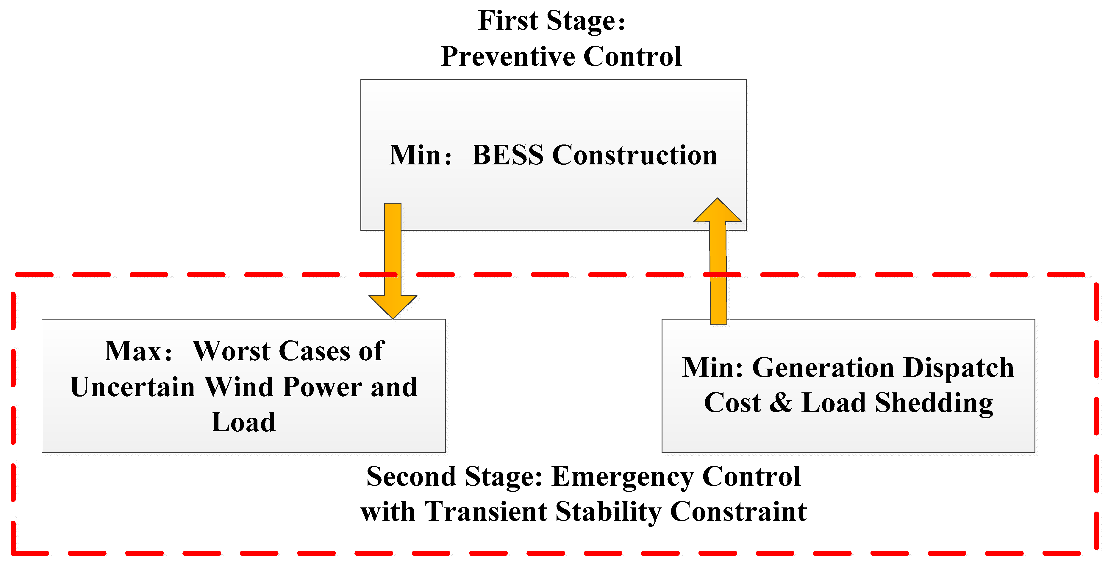
4]. In practice, in order to enhance transient stability, control strategies can be divided into preventive control (PC) and emergency control (EC) according to the different implementation time. Preventive control, such as optimal scheduling of generator sets, aims to prepare the system before unexpected events occur. Emergency control, such as load shedding, is to try to avoid loss of synchronization of a power system after contingencies [5].
The existing classical transient stability research is mainly focused on simulation models. Furthermore, the time domain simulation (TDS) method based on engineering experience has been widely applied in industries [6,7,8]. This method has the disadvantage of a large amount of computation. Another method is to terminate time-domain simulation in advance and determine the criteria for premature termination according to the characteristics of transient stability [9]. However, these rules are only enhanced on the basis of direct methods for transient stability analysis [10,11] including instantaneous energy function (TEF) method [12,13], extended equal area criterion (EEAC) method [14], and trajectory concave-convex method (TCC) [15].
Artificial-intelligence-based algorithms have also been used for transient stability forecasting. In [16], the authors developed an improved decision tree (DE) for dynamic test by synchronous phasors. In the literature [17], lasso regression (LR) was applied to forecast stability interval. In [18], voltage, speed, and power angle of generator were used by support vector machine (SVM) to forecast transient stability index (TSI). In [19], first-order regression was used to investigate system uncertainty variables. Extreme gradient boosting (XGBoost) and factorization machine (FM) were applied for transient stability assessment of power systems [20]. Improved SVM was used for online system assessment [21]. Further, [22] proposed a novel l deep-machine-learning-based model for power system forecasting.
In addition, artificial neural networks (ANNs) have been applied for power systems [23,24]. However, the conventional artificial intelligence algorithms are very bounded in their ability to deal with modern power systems. To overcome these problems, deep learning models have been developed and applied to many fields. For example, in the literature [25,26,27,28], stack denoising autoencoder (SDA), convolutional neural network (CNN), and reinforcement learning (RL) have been applied to transient stability prediction. However, when it comes to transient stability analysis, the performance of these conventional algorithms will be weakened because the specific topological structure of the system data and information transfer between bus nodes are ignored.
The best operation dispatch of the system before an accident can be achieved is by optimal power flow calculation considering the transient stability constraint. Therefore, optimal scheduling of the generator set in preventive control is very suitable for stability enhancement of the power system [29,30,31,32,33,34]. The probability of an accident in a power system is low in long-term operation, so the cost of preventive controls will be high. Short-term emergency controls may also be costly, but the probability of implementation is very low. Therefore, cost-effectiveness of emergency controls is also a factor to be considered. In [35], an optimized load shedding scheme is proposed to improve the transient stability and frequency/voltage stability of a power system. In [36], in order to improve the transient stability of a system, a risk-based coordination model is adopted to model generation rescheduling and emergency load reduction. However, these studies based on preventive control and emergency control cannot consider uncertainties of alternative energies, such as wind and PV. At the same time, the transient stability control model mentioned above cannot guarantee complete robustness.
From the above literature review, it is clear that the research on transient stability coordinated preventive and emergency control based on the latest artificial intelligence algorithm is still in the initial stage, and there are many theoretical and technical difficulties that have not been solved. For example, the algorithms used in the above research cannot consider the specific data of electric power system topology, node, and information transmission. In addition, some algorithms can lead to a huge amount of calculation, and transient stability forecasting by traditional machine learning methods does not address how to use the prediction results for future control. Even fewer studies have considered cooperative control to improve transient stability.
Considering that the more diversified and generalized alternative energies in a modern system will easily affect the system stability, the existing transient stability research models and optimization algorithms in the literature would not meet future requirements. How to consider both preventive and emergency control has not been well dealt with in the existing models. Some theoretical difficulties, such as global convergence of the optimization scheduling algorithm and stability and robustness of the control algorithm, are still lacking thorough study. Based on the above considerations, this paper will systematically study coordinated preventive and emergency control based on the latest artificial intelligence algorithm.
The proposed paper contributions are as follows:
(1)
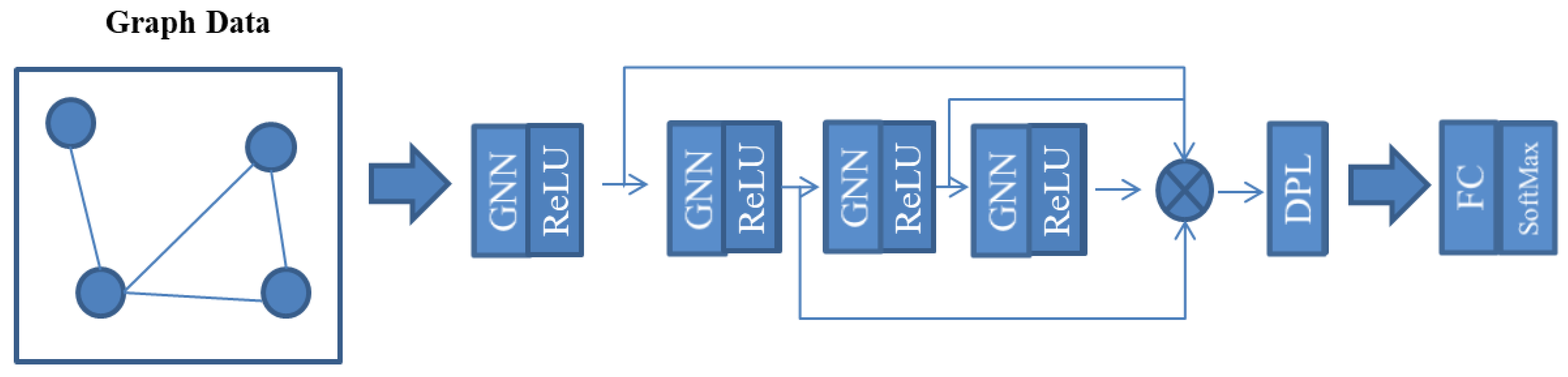
The main theoretical innovation of this paper is that it clearly points out the significant influence of cooperative preventive control and emergency control on system stability and proposes a two-stage robust cooperative control model based on distributed preserving graph representation learning (DPG). According to the worst scenario of the model, transient stability index (TSI) and robust global optimization results can be accurately derived. This idea is obviously different from the existing studies, which only control transient stability and do not pay attention to the special results of the system.
(2)
The main algorithm innovation is that this paper proposes a modified column and constraint generation (C&CG) [37] method, which is the traditional C&CG framework combined with deep-learning-based transient stability constraints. This method is our original algorithm and has high theoretical value.
The rest of this paper is organized as follows. The proposed coordinated system control strategy is introduced in Section 2. The proposed mathematical framework is presented in Section 3. The solution method is presented in Section 4. The case studies are developed in Section 5, and Section 6 provides the conclusion.

2. Cooperative Transient Stability Control Strategy

2.1. Two-Stage Robust Optimization Model

Two-stage robust optimization algorithm has been proven to be a valid method to handle uncertainty and robustness. This method has been widely used in economic dispatch considering uncertainty and economic dispatch with fault constraints [38,39,40]. At the same time, when uncertainty is considered, the two-stage robust optimization algorithm also shows good robustness in operation of microgrids [41,42,43].
Therefore, as shown in Figure 1, aiming at transient instability of the system considering uncertain wind output and demand load, this paper proposes a collaborative control optimization method. The strategy is modeled as an adjustable robust optimization framework with distributed preserving graph representation learning (DPG)-based transient stability constraint. In the first stage, BESS construction is optimized before the contingences. In the second stage, the decisions are generation scheduling and load shedding after the contingences in the worst cases of wind generation and load changes. In order to solve this proposed model, a novel solution method that constructs the stability constraint in the columns and constraint generation algorithm framework is researched.

2.2. Uncertainty Set Modelling

It is considered that the fluctuation range of wind generation and load power can be described as the uncertainty sets:
U = { u = [ u W ( t ) ,     u L ( t ) ] T ,     t = 1 , 2 , , N T u W ( t ) [ u W ( t ) Δ u W max ( t ) ,     u W ( t ) + Δ u W max ( t ) u L ( t ) [ u L ( t ) Δ u L max ( t ) ,     u L ( t ) + Δ u L max ( t ) }
Here, u W ( t ) and u L ( t ) are the uncertain variables of wind generation and load. u W max ( t ) and Δ u L max are the maximum fluctuation range of wind power output and load.

2.3. Transient Stability Index (TSI) Prediction Algorithm Based on Distribution Preserving Graph Representation Learning (DPG)

In distribution network analysis, distribution network is usually abstracted as a graph model for the convenience of subsequent analysis. The power grid contains a variety of power equipment, such as bus bars, lines, transformers, generators, loads, switches, etc. In the process of power grid modeling, the objects are all kinds of physical equipment of the power system, such as lines, transformers, generators, etc. The system modeling can be described in Figure 2. In the task scenario of this paper, an undirected graph model can be constructed by selecting the configuration variable as the node in the graph and the lines connected between each configuration variable as the edge in the graph.
In Figure 2, each node represents a bus with transient stability index (TSI) information and the node attribute is TSI sequence data. Each bus is connected by a line. The graph model can be used as an abstraction of the real power grid, which can facilitate subsequent tasks.
Considering the special system topology and distribution information of bus nodes, a graph neural network (GNN) model embedded with distribution preserving learning (DPL), which is distribution preserving graph representation learning (DPG), is developed. The pooling operation of DPG can accurately learn and describe the representation of the entire node distribution (determination of the system state). The final representation will be helpful to obtain a more accurate prediction and significantly improve the computational efficiency while maintaining high accuracy. By means of DPG, we can determine the relationship between TSI and power system operation characteristics so as to ensure the transient stability of the model under coordinated control.
TSI based for generator rotor angle is selected to describe system stability or fault severity, and TSI is defined as follows [44,45,46]:
TSI = ( 360 | Δ δ max | ) × 100 360 + | Δ δ max |
where Δ δ max represents the maximum angle difference of the power system. When TSI > 0, the system is treated as transient stable, including critical stable; otherwise, the system becomes unstable.

3. Mathematical Formulation

Coordinated control model is developed in our paper. A transient stability constrained optimization model of cooperative preventive control and emergency control is an adaptive robust problem where the BESS investment plan is chosen in the prevention stage before the contingence. In the lower stage, the contingence is considered. If a construction plan of BESS can meet the fluctuation deviation of wind power output and load under the contingence, the system can measure against all other scenarios.
min x ( i I c i B E S S x i                                           max u U             min y Ω ( x , u )           (   g i G t T c g i p p g i t + i I t T c i d p d i t     ) )  
Subject to:
i I c i B E S S x i B E S S
( x i ) { 0 , 1 }
  g i G i p g i t j B i , j ( θ i t θ j t ) + w i p w i t =   d i t + r c h , i t / η c h r d c h , i t η d c h + p d i t ,                                                                                                                                               i I ,     g i G , w i G w , t T
F i , j min B i , j ( θ i t θ j t ) F i , j max ,   ( i , j ) L , t T
p g i min p g i t p g i max , g i G i , t T
D R p g i t p g i t 1 U R ,     g i G i , t T
p d i min p d i t p d i max , i I , t T
θ i min θ i t θ i max , i I , t T        
S O C i t = S O C i t 1 + r c h , i t η c h r d c h , i t / η d i s ,     i I , t T \ { 1 }
S O C i 1 = S 0 + r c h , i 1 η c h r d c h , i 1 / η d i s
S O C T = S f = S 0
[ x i ] S O C i min S O C i t [ x i ] S O C i max ,     i I , t T
r c h , i t r c h , i max ,       i I , t T
r d c h , i t r d c h , i max ,     i I , t T
i I p d i t p d ,     i I ,     t T
w i p w i t = u w ( t ) , t T
i I d i t = u L ( t ) , t T
L ( Λ t ) > T S I B , t T
Equation (3) tries to minimize the construction cost of BESS in the preventive control stage and the system operation and load shedding cost under the worst-case scenario of wind energy and load in the emergency control stage. Constraint (4) represents the budget constraints for the BESS investments. The 0/1 variables in Constraint (5) are used to show whether a BESS construction is undertaken in a node (e.g., 1 means a construction is chosen). Constraint (6) is the node power balance equation that represents DC power flow at the preventive control state. Constraint (7) is the branch power flow limit equation. Constraint (8) presents the power output limits. Unit climbing constraint equation is described in Constraint (9). Constraint (10) denotes the emergency load shedding limits at the emergency control state. Constraint (11) limits phase angles of transmission lines. Constraint (12) describes the charge and discharge stage of the BESS except for the initial time. Constraint (13) presents the BESS state of charge in the first time step. Constraint (14) means that the final BESS state of charge is equal to the initial BESS state of charge. Constraint (15) provides the BESS minimum and maximum capacity. Constraint (16) and (17) describe the BESS charge and discharge rate limits, respectively. Constraint (18) limits the load shedding budget. Constraint (19) and (20) mean that the wind energy and load are equal to the values of uncertain variables corresponding to each time period. Equation (21) is the developed transient stability constraint.

4. Solution Methodology

4.1. Compact Matrix Form

Normally, an adaptive robust optimization model can be solved by C&CG method. However, this paper proposed a novel coordinated preventive and emergency control framework with transient stability constraint. As a result, the traditional C&CG method cannot be directly used. This paper investigated an improved C&CG algorithm that can solve the modified two-stage proposed model.
The compact form of the coordinated transient stability control model can be represented as below:
min x ( c 1 T x + max u U min y Ω ( x , u ) c 2 T y )
where x and y are the requirement variables and the detailed form can be denoted as follows:
{ x = [ x i ] T y = [ p g i t , p d i t , p w i t , d i t , θ i t , S O C i t , r c h , i t , r d c h , i t ] T ,             t = ( 1 , 2 N T )
where the requirement variable of the first stage is x and the requirement variables of the second stage are u and y. The minimum problem of the inner layer is equivalent to objective Equation (3), which represents the minimum system operation budget. The expressions of x and y are shown in Equation (23). Ω(x, u) is the feasible zone of requirement variable y, and the detailed expression can be described as follows:
s . t .     Ω ( x , u ) = { A x e ,     x { 0 , 1 }             λ 1
D y d           λ 2
K y = k           λ 3
F x + G y h           λ 4
H y = u           λ 5 }
Here, variables c1 and c2 are the parameter vectors of Equation (3). A, D, K, F, G, and H are the parameter matrixes of the variables for the corresponding constraints, and e, d, k, h, and u are the constant columns vectors. Equation (24) corresponds to Equations (4) and (5). Equation (25) represents inequality constraints in the developed adjustable robust model, including Equations (7)–(11) and (16)–(18). Equation (26) represents equality constraints in the proposed model, including Equations (6), (12)–(14), (19), and (20). Equation (27) corresponds to Equation (15). Equation (28) shows that, in the proposed model, the values of wind energy and load are the corresponding uncertain values in each time period. Λ1, λ2, λ3, λ4, and λ5 are the dual variables corresponding to each constraint in the lower stage.

4.2. Model Framework Reformulation

In terms of the developed adaptive optimization model, column constraint generation algorithm (C&CG) is used to solve the proposed problem. After decomposition of Equation (22), the main problem can be written as:
min x c 1 T x + η
s . t .       η c 2 T y l
A x e ,     x { 0 , 1 }
D y l d
K y l = k
F x + G y l h
H y l = u l *
l j
where j is the current iteration; yl is the solution of the subproblem after the lth loop. u l * is the value of variable u in the worst contingence achieved after the lth loop.
The subproblem can be expressed as follows:
max u U min y Ω ( x , u ) c 2 T y
The Equation (22) can be converted into the following dual problem:
max u U , λ 1 λ 5 e T λ 1 + d T λ 2 + k T λ 3 + ( h F x ) T λ 4 + u T λ 5
s . t .       A λ 1 + D λ 2 + K λ 3 + G λ 4 + H λ 5 c 2
λ 1 λ 5 0
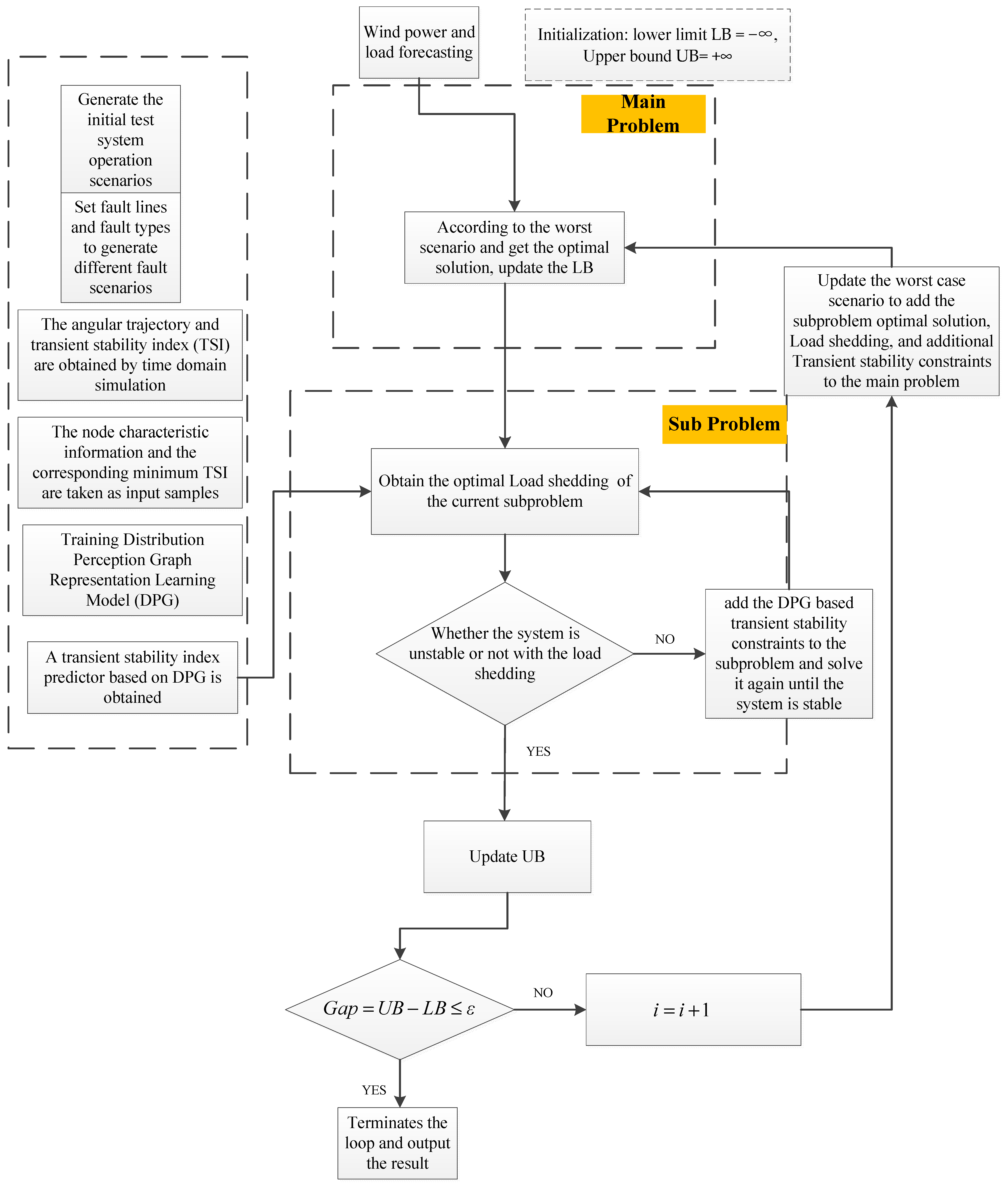
The developed model is finally decoupled into the main problem corresponding to Formulas (29)–(36) and sub-problem corresponding to Formulas (38)–(40) with mixed integer linear form. However, the researched coordinated control model includes transient stability constraint. As a result, the model cannot be directly solved by traditional C&CG method. Therefore, we proposed a novel solution that combines the original C&CG method with transient stability assessment to solve the developed model. The process of the improved solution algorithm is as follows:
(1)
Given the values of a group of uncertain variables as the initial worst contingence, set the operational cost lower limit LB = −∞, the upper bound UB = +∞, corresponding to the final dispatch scheme, and the iteration number k = 1;
(2)
Solve the main problem formulas (29)–(36) according to the worst contingence u 1 * , and obtain the solution ( x k * , η k * ), where the objective equation value of the main problem is taken as the new lower limit LB = c 1 T x + η ;
(3)
Substitute the obtained main problem solution x k * into Equations (38)–(40), solve the subproblem, obtain the value of the objective equation f k * ( x k * ) of the subproblem, the value of the corresponding uncertainty variable u in the worst contingency, which is u k + 1 * , and the second stage variable value of load shedding, which is y k * ;
(4)
If the system is unstable with the load shedding amount, add the DPG-based transient stability constraint to the subproblem and solve it again until the system is stable;
(5)
Update the upper limit UB = min {UB, f k * ( x k * ) }, The convergence threshold is ε, If UB − LB ≤ ε, then stop the loop and return solutions x k * and y k * ; otherwise, add variable y k + 1 and the following constraints to the master problem:
{ η c 2 T y k + 1 D y k + 1 d K y k + 1 = k F x + G y k + 1 h H y k + 1 = u k + 1 *
(6)
Set k = k + 1; go to step 2 until the method meets the condition of the convergence.
The flowchart of the developed novel solution algorithm including the original C&CG method with transient stability constraints is shown in Figure 3.

5. Case Studies

The proposed coordinated transient stability control model is illustrated on the modified IEEE 30 and 39 bus system [47]. To build the data-driven model proposed in this paper, data under various transient scenarios are needed for training. However, the probability of fault scenarios in actual operation is very low, and it is difficult to collect data under various transient fault scenarios. Therefore, MATPOWER [48] and Power System Analysis Toolbox (PSAT) [49] are used for simulation. The improved IEEE 30 and 39 bus system are adopted. On the basis of the original IEEE 30 bus system, a wind power plant model based on PSAT software package and equivalent to multiple doubly fed wind turbines is added at bus node 17, and the same wind power model is added at bus 32 of IEEE 39 bus system.

5.1. Construction of the Training Dataset

The developed two-stage robust optimization framework is implemented on the improved IEEE 30 system. The test system includes 6 generators, 41 transmission lines, and 21 system loads. Select 10 lines from all lines of the benchmark system as the predicted fault lines; set the single-phase short circuit fault to form the predicted fault set. The predicted fault sets are shown in Table 1 and Table 2.
The power generation is set to fluctuate within 90–110%. A thousand kinds of generator active power outputs are generated by Latin Hypercube sampling, and the system load active power and reactive power fluctuate with the change in the total active power output of the generator. The 1000 kinds of generator active power outputs and 10 expected fault lines in the expected fault set are combined to form 10,000 kinds of expected fault data. PSAT is used for time domain simulation calculation of the expected fault data, and the fault removal time is set as 0.1 s and the total simulation time as 20 s. The corresponding TSI is solved. The output of each generator corresponds to 10 TSIs, and the smallest TSI among the 10 TSIs is selected. Together with the output of this generator, 1000 sample data are formed for training the deep-learning-based transient stability predictor.

5.2. Transient Stability Predictor

The 1200-sample dataset was divided into a 960-sample training dataset and a 240-sample test dataset. The transient stability predictor was trained using the training set, and the accuracy of the model was verified by the test set.
As illustrated in Figure 4, considering the bus nodes as the vertices and the lines as the edges, we can transform the power node system into a graph neural network structure. Then, we use the GNN (graph neural networks) and ReLU (rectified linear unit) to obtain the information for the bus nodes. According to the learned node characteristics, such as active power, reactive power, voltage, and phase angle, we apply the proposed DPG model to describe the information distribution among bus nodes so as to learn the information graphic representation used to describe the state of the power system. Finally, the obtained representations can be used as inputs to common prediction models to realize transient stability analysis.
In order to verify the effectiveness of the proposed DPG method [50], we conducted a comparative simulation test with six different popular machine learning algorithms. In addition, different precision indexes, such as accuracy, F1 score, and true negative rate (TNR), were used to measure performance.
From Table 3, we can see that the developed distribution preserving graph representation learning (DPG) algorithm performs best for all the forecasting precision indexes. The main reason is that the proposed DPG method considers the topology of power system data structures as the main consideration, which can significantly improve the computation effectiveness.

5.3. Analysis of Coordinated Transient Stability Control Results

5.3.1. Generators Active Power Outputs Analysis

The DPG-based transient stability predictor is embedded into the two-stage robust optimization to control the outputs of transient unstable generators. In terms of IEEE 30 and 39 bus system, generators’ outputs before and after collaborative control are shown in Table 4 and Table 5, respectively.
From Table 4 and Table 5, the average generators power outputs decreased after the coordinated transient stability control. It is also worth mentioning that the total operation cost also dropped because of the decreased power outputs.

5.3.2. Transient Stability Index (TSI) Analysis

Finally, PSAT was used to verify the collaborative control strategy, and the time-domain simulation method was used to calculate the TSI before and after the collaborative control under each expected fault. The TSI pairs before and after the collaborative control of the IEEE 30 and 39 test systems were shown in Table 5 and Table 6, respectively.
As can be seen from Table 6 and Table 7, the faults that are transient unstable before collaborative control become transient stable after collaborative control, while the faults that are transient stable before collaborative control remain transient stable. It also can be seen that TSIs are slightly improved, which can indicate that the coordinated control strategy also appropriately increases the system transient stability margin for the full fault set.

5.3.3. Rotor Angles and Voltage Curves Analysis

Table 8 shows two contingency scenarios for different fault lines of IEEE 39 bus system. We perform scenario 1 and scenario 2 for the simulation, and the generator rotor angles and voltages are shown in the following figures.
Figure 5 and Figure 6 show the power angle curves before and after collaborative control of the IEEE 39 system under single-phase short circuit fault of the lines (bus 25 to bus 26; bus 26 to bus 29); it is clear that the benchmark test system is unstable since the collaborative transient stability control is not performed. However, the system changed to stable after the collaborative control.
Figure 7 and Figure 8 show the voltage curves before and after collaborative control of the IEEE 39 bus system under single-phase short circuit fault of the line (bus 25 to bus 26; bus 26 to bus 29); the test system is unstable since the collaborative transient stability control is not carried out. However, the system changed to stable after the collaborative control. The voltage curves further validate the effectiveness of the proposed collaborative transient stability control.

6. Conclusions

In this paper, distribution preserving graph representation learning (DPG) and two-stage robust optimization framework were introduced into a transient stability cooperative control model and a deep-learning-driven improved algorithm for transient stability coordinated control of power systems was proposed. The proposed improved algorithm includes a set of transient stability predictors based on DPG and accurately fits the mapping relationship between generator outputs and transient stability index (TSI) by the training method of “unsupervised pre-training-parameter optimization”. Different from conventional artificial intelligence algorithms, this paper embedded the trained transient stability predictor as a “black-box constraint” into the iterative optimization process of two-stage robust optimization. A data-driven optimization technique for the cooperative control strategy of generation rescheduling and load shedding with the goal of controlling cost minimization was proposed in this paper.
This research work developed a novel approach for transient stability collaborative control. It also provides reference for embedding similar power system stability rules into corresponding control models.

Author Contributions

F.Y. proposed the methodological framework and mathematical model and performed the simulations; X.Z. modified and improved the mathematical model; T.K.C. examined the mathematical model, analyzed the results, reviewed the manuscript, and provided suggestions; H.H.-c.I. examined the mathematical model, reviewed the manuscript, and provided suggestions. All authors have read and agreed to the published version of the manuscript.

Funding

This work is supported by Research Project Supported by Shanxi Scholarship Council of China (Project Number: 2022-005).

Data Availability Statement

Data available on request from the authors.

Conflicts of Interest

The authors declare no conflict of interest.

Nomenclature

A. Set
ISet of all buses.
G Set of generators.
T Set of time horizon.
B. Parameters
B E S S Construction budget for BESS.
p d Upper limit of load shedding.
B i , j Susceptance of branch (i, j).
c i B E S S Construction cost for BESS at bus i.
c g i p Generation cost of generator g at bus i.
c i d Cost of load shedding at bus i.
F i , j min Lower bound of branch power flow capacity.
F i , j max Upper bound of branch power flow capacity.
p g i max Upper generation limit of generator g at bus i.
p g i min Lower generation limit of generator g at bus i.
p d i max Upper load shedding limit at bus i.
p d i min Lower load shedding limit at bus i.
θ i max Maximum rotor angle at bus i.
θ i min Minimum rotor angle at bus i.
S O C i max Maximum state of charge at bus i.
S O C i min Minimum state of charge at bus i.
r c h , i max Maximum charge amount at bus i.
r d c h , i max Maximum discharge amount at bus i.
η c h Charge factor of BESS.
η d c h Discharge factor of BESS.
C.Decision Variables
x i On–off variable for BESS construction.
θ i t Phase angle at bus i in time step t .
S O C i t State of charge at bus i in time step t .
p d i t Load shedding at bus i in time step t .
p g i t Power output of unit g at bus i in time step t .
r c h , i t The charge power of BESS at bus i in time step t .
r d c h , i t The discharge power of BESS at bus i in time step t .

References

  1. Strbac, G.; Pudjianto, D.; Aunedi, M.; Papadaskalopoulos, D.; Djapic, P.; Ye, Y.; Moreira, R.; Karimi, H.; Fan, Y. Cost-Effective Decarbonization in a Decentralized Market: The Benefits of Using Flexible Technologies and Resources. IEEE Power Energy Mag. 2019, 17, 25–36. [Google Scholar] [CrossRef]
  2. Sayed, A.R.; Wang, C.; Bi, T. Resilient operational strategies for power systems considering the interactions with natural gas systems. Appl. Energy 2019, 241, 548–566. [Google Scholar] [CrossRef]
  3. Australian Energy Market Operator. Black System South Australia 28 September 2016. 2017. Available online: https://www.aemo.com.au/-/media/Files/Electricity/NEM/Market_Notices_and_Events/Power_System_Incident_Reports/2017/Integrated-Final-Report-SA-Black-System-28-September-2016.pdf (accessed on 6 January 2023).
  4. Kundur, P.; Paserba, J.; Ajjarapu, V.; Andersson, G.; Bose, A.; Canizares, C.; Hatziargyriou, N.; Hill, D.; Stankovic, A.; Taylor, C.; et al. Definition and Classification of Power System Stability IEEE/CIGRE Joint Task Force on Stability Terms and Definitions. IEEE Trans. Power Syst. 2004, 19, 1387–1401. [Google Scholar] [CrossRef]
  5. Yuan, H.; Xu, Y. Preventive-Corrective Coordinated Transient Stability Dispatch of Power Systems with Uncertain Wind Power. IEEE Trans. Power Syst. 2020, 35, 3616–3626. [Google Scholar] [CrossRef]
  6. Adibi, M.; Hirsch, P.; Jordan, J. Solution methods for transient and dynamic stability. Proc. IEEE 1974, 62, 951–958. [Google Scholar] [CrossRef]
  7. Gan, D.; Thomas, R.J.; Zimmerman, R.D. Stability-constrained optimal power flow. IEEE Trans. Power Syst. 2000, 15, 535–540. [Google Scholar] [CrossRef] [Green Version]
  8. Diao, R.; Jin, S.; Howell, F.; Huang, Z.; Wang, L.; Wu, D.; Chen, Y. On Parallelizing Single Dynamic Simulation Using HPC Techniques and APIs of Commercial Software. IEEE Trans. Power Syst. 2017, 32, 2225–2233. [Google Scholar] [CrossRef]
  9. Kamwa, I.; Grondin, R.; Loud, L. Time-varying contingency screening for dynamic security assessment using intelli-gent-systems techniques. IEEE Trans. Power Syst. 2001, 16, 526–536. [Google Scholar] [CrossRef]
  10. Chang, H.D.; Chu, C.C.; Cauley, G. Direct stability analysis of electric power systems using energy functions: Theory, applications, and perspective. Proc. IEEE 1995, 83, 1497–1529. [Google Scholar] [CrossRef]
  11. Bhui, P.; Senroy, N. Real Time Prediction and Control of Transient Stability Using Transient Energy Function. IEEE Trans. Power Syst. 2017, 32, 923–934. [Google Scholar] [CrossRef]
  12. Xue, Y. Fast analysis of stability using EEAC and simulation technologies. In Proceedings of the POWERCON’98. 1998 International Conference on Power System Technology, proceedings (Cat. No.98EX151), Beijing, China, 18-21 August 1998. [Google Scholar] [CrossRef]
  13. Su, F.; Yang, S.; Wang, H.; Zhang, B. Study on fast termination algorithm of time-domain simulation for power system transient stability. Proc. CSEE 2017, 15, 4372–4378. [Google Scholar]
  14. Vu, T.L.; Al Araifi, S.M.; El Moursi, M.S.; Turitsyn, K. Toward simulation-free estimation of critical clearing time. IEEE Trans. Power Syst. 2016, 31, 4722–4731. [Google Scholar] [CrossRef] [Green Version]
  15. Geeganage, J.; Annakkage, U.D.; Weekes, T.; Archer, B.A. Archer Application of energy-based power system features for dynamic security assessment. IEEE Trans. Power Syst. 2015, 30, 1957–1965. [Google Scholar] [CrossRef] [Green Version]
  16. Sun, K.; Likhate, S.; Vittal, V.; Kolluri, V.S.; Mandal, S. An online dynamic security assessment scheme using phasor measurements and decision trees. IEEE Trans. Power Syst. 2007, 22, 1935–1943. [Google Scholar] [CrossRef]
  17. Lv, J.; Pawlak, M.; Annakkage, U.D. Prediction of the Transient Stability Boundary Using the Lasso. IEEE Trans. Power Syst. 2013, 28, 281–288. [Google Scholar] [CrossRef]
  18. Gomez, F.R.; Rajapakse, A.D.; Annakkage, U.D.; Fernando, I.T. Support vector machine-based algorithm for post-fault transient stability status prediction using synchronized measurements. IEEE Trans. Power Syst. 2011, 26, 1474–1483. [Google Scholar] [CrossRef]
  19. Daniels, C.C.; Garafolo, N.G. Effect of system variables on the uncertainty of the mass point leak rate methodology using first-order regression. Nondestruct. Test. Eval. 2014, 29, 14–28. [Google Scholar] [CrossRef]
  20. Li, N.; Li, B.; Gao, L. Transient Stability Assessment of Power System Based on XGBoost and Factorization Machine. IEEE Access 2020, 8, 28403–28414. [Google Scholar] [CrossRef]
  21. Hu, W.; Lu, Z.; Wu, S.; Zhang, W.; Dong, Y.; Yu, R.; Liu, B. Real-time transient stability assessment in power system based on improved SVM. J. Mod. Power Syst. Clean Energy 2019, 7, 26–37. [Google Scholar] [CrossRef] [Green Version]
  22. Zhu, L.; Hill, D.J.; Lu, C. Hierarchical Deep Learning Machine for Power System Online Transient Stability Prediction. IEEE Trans. Power Syst. 2020, 35, 2399–2411. [Google Scholar] [CrossRef]
  23. Siddiqui, S.A.; Verma, K.; Niazi, K.R.; Fozdar, M. Real-Time Monitoring of Post-Fault Scenario for Determining Generator Coherency and Transient Stability Through ANN. IEEE Trans. Ind. Appl. 2018, 54, 685–692. [Google Scholar] [CrossRef]
  24. Lajimi, R.A.; Amraee, T. A two stage model for rotor angle transient stability constrained optimal power flow. Int. J. Electr. Power Energy Syst. 2016, 76, 82–89. [Google Scholar] [CrossRef]
  25. Zhu, Q.; Chen, J.; Zhu, L.; Shi, D.; Bai, X.; Duan, X.; Liu, Y. A Deep End-to-End Model for Transient Stability Assessment with PMU Data. IEEE Access 2018, 6, 65474–65487. [Google Scholar] [CrossRef]
  26. Yan, R.; Geng, G.; Jiang, Q.; Li, Y. Fast transient stability batch assessment using cascaded convolutional neural networks. IEEE Trans. Power Syst. 2019, 34, 2802–2813. [Google Scholar] [CrossRef]
  27. Yoon, D.; Hong, S.; Lee, B.J.; Kim, K.E. Winning the l2rpn challenge: Power grid management via semi-markov afterstate actorcritic. In Proceedings of the International Conference on Learning Representations, Virtual Conference, 26 April–1 May 2020. [Google Scholar]
  28. Li, X.; Li, H.; Li, S.; Jiang, Z.; Ma, X. Review on Reactive Power and Voltage Optimization of Active DistributionNetwork with Renewable Distributed Generation and Time-Varying Loads. Math. Probl. Eng. 2021, 2021, 1–18. [Google Scholar]
  29. Nguyen, T.; Pai, M. Dynamic security-constrained rescheduling of power systems using trajectory sensitivities. IEEE Trans. Power Syst. 2003, 18, 848–854. [Google Scholar] [CrossRef] [Green Version]
  30. Pizano-Martinez, A.; Fuerte-Esquivel, C.R.; Ruiz-Vega, D. A New Practical Approach to Transient Stability-Constrained Optimal Power Flow. IEEE Trans. Power Syst. 2011, 26, 1686–1696. [Google Scholar] [CrossRef]
  31. Zarate-Minano, R.; Van Cutsem, T.; Milano, F.; Conejo, A.J. Securing Transient Stability Using Time-Domain Simulations within an Optimal Power Flow. IEEE Trans. Power Syst. 2010, 25, 243–253. [Google Scholar] [CrossRef] [Green Version]
  32. Xu, Y.; Dong, Z.Y.; Zhao, J.; Xue, Y.; Hill, D.J. Trajectory sensitivity analysis on the equivalent one-machine-infinite-bus of multi-machine systems for preventive transient stability control. IET Gener. Transmiss. Distrib. 2015, 9, 276–286. [Google Scholar] [CrossRef]
  33. Xu, Y.; Dong, Z.Y.; Meng, K.; Zhao, J.H.; Wong, K.P. A Hybrid Method for Transient Stability-Constrained Optimal Power Flow Computation. IEEE Trans. Power Syst. 2012, 27, 1769–1777. [Google Scholar] [CrossRef]
  34. Xu, Y.; Dong, Z.Y.; Xu, Z.; Zhang, R.; Wong, K.P. Power system transient stability-constrained optimal power flow: A comprehensive review. In Proceedings of the 2012 IEEE Power and Energy Society General Meeting, San Diego, CA, USA, 22–26 July 2012; pp. 1–7. [Google Scholar] [CrossRef]
  35. Xu, X.; Zhang, H.; Li, C.; Liu, Y.; Li, W.; Terzija, V. Optimization of the Event-Driven Emergency Load-Shedding Considering Transient Security and Stability Constraints. IEEE Trans. Power Syst. 2017, 32, 2581–2592. [Google Scholar] [CrossRef]
  36. Wang, Z.; Song, X.; Xin, H.; Gan, D.; Wong, K.P. Risk-Based Coordination of Generation Rescheduling and Load Shedding for Transient Stability Enhancement. IEEE Trans. Power Syst. 2013, 28, 4674–4682. [Google Scholar] [CrossRef]
  37. Zeng, B.; Zhao, L. Solving two-stage robust optimization problems using a column-and-constraint generation method. Oper. Res. Lett. 2013, 41, 457–461. [Google Scholar] [CrossRef]
  38. Chen, Y.; Zhang, Z.; Chen, H.; Zheng, H. Robust UC model based on multi-band uncertainty set considering the temporal correlation of wind/load prediction errors. IET Gener. Transm. Distrib. 2020, 14, 180–190. [Google Scholar] [CrossRef]
  39. Chen, Y.; Zhang, Z.; Liu, Z.; Zhang, P.; Ding, Q.; Liu, X.; Wang, W. Robust Nk CCUC model considering the fault outage probability of units and transmission lines. IET Gener. Transm. Distrib. 2019, 13, 3782–3791. [Google Scholar] [CrossRef]
  40. Bertsimas, D.; Litvinov, E.; Sun, X.A.; Zhao, J.; Zheng, T. Adaptive Robust Optimization for the Security Constrained Unit Commitment Problem. IEEE Trans. Power Syst. 2013, 28, 52–63. [Google Scholar] [CrossRef]
  41. Zhang, C.; Xu, Y.; Dong, Z.Y.; Ma, J. Robust Operation of Microgrids via Two-Stage Coordinated Energy Storage and Direct Load Control. IEEE Trans. Power Syst. 2017, 32, 2858–2868. [Google Scholar] [CrossRef]
  42. Zhang, C.; Xu, Y.; Dong, Z.Y. Robustly Coordinated Operation of a Multi-Energy Micro-Grid in Grid-Connected and Islanded Modes Under Uncertainties. IEEE Trans. Sustain. Energy 2020, 11, 640–651. [Google Scholar] [CrossRef]
  43. Zhang, C.; Xu, Y.; Dong, Z.Y.; Wong, K.P. Robust Coordination of Distributed Generation and Price-Based Demand Response in Microgrids. IEEE Trans. Smart Grid 2018, 9, 4236–4247. [Google Scholar] [CrossRef]
  44. Zhang, R.; Xu, Y.; Dong, Z.Y.; Wong, K.P. Post-disturbance transient stability assessment of power systems by a self-adaptive intelligent system. IET Gener. Transm. Distrib. 2015, 9, 296–305. [Google Scholar] [CrossRef]
  45. Genc, I.; Diao, R.; Vittal, V.; Kolluri, S.; Mandal, S. Decision Tree-Based Preventive and Corrective. Control Applications for Dynamic Security Enhancement in Power Systems. IEEE Trans. Power Syst. 2010, 25, 1611–1619. [Google Scholar] [CrossRef]
  46. Su, T.; Liu, Y.; Zhao, J.; Liu, J. Deep Belief Network Enabled Surrogate Modeling for Fast Preventive Control of Power System Transient Stability. IEEE Trans. Ind. Inform. 2022, 18, 315–326. [Google Scholar] [CrossRef]
  47. Venkatesh, P.; Lee, K.Y. Multi-Objective Evolutionary Programming for Economic Emission Dispatch problem. In Proceedings of the 2008 IEEE Power and Energy Society General Meeting-Conversion and Delivery of Electrical Energy in the 21st Century, Pittsburgh, PA, USA, 20–24 July 2008. [Google Scholar] [CrossRef]
  48. Ray, D.Z.; Carlos, E.M. Matpower: A MATLAB Power System Simulation Package, Mar. 2018. [Online]. Available online: http://www.pserc.cornell.edu/matpower/ (accessed on 5 January 2023).
  49. Milano, F. Power System Analysis Toolbox (PSAT), March 2018. Available online: http://faraday1.ucd.ie/index.html (accessed on 6 January 2023).
  50. Mian, T.; Choudhary, A.; Fatima, S. Vibration and infrared thermography based multiple fault diagnosis of bearing using deep learning. Nondestruct. Test. Eval. 2022, 8, 1–22. [Google Scholar] [CrossRef]
Figure 1. The two-stage/tri-level model developed for cooperative transient stability control.
Energies 16 02413 g001
Figure 2. Constructing power system structure into graph structure.
Energies 16 02413 g002
Figure 3. The flowchart of the developed novel solution algorithm.
Energies 16 02413 g003
Figure 4. The illustration of the proposed distribution preserving graph representation learning (DPG).
Energies 16 02413 g004
Figure 5. Comparison of rotor angle curve before and after collaborative transient stability control on fault lines 25−26 of IEEE 39 bus system.
Energies 16 02413 g005
Figure 6. Comparison of rotor angle curve before and after collaborative transient stability control on fault lines 26−29 of IEEE 39 bus system.
Energies 16 02413 g006
Figure 7. Comparison of voltage curve before and after collaborative transient stability control on fault lines 25–26 of IEEE 39 bus system.
Energies 16 02413 g007
Figure 8. Comparison of voltage curve before and after collaborative transient stability control on fault lines 26–29 of IEEE 39 bus system.
Energies 16 02413 g008
Table 1. Contingency set of IEEE 30 bus system.
Fault Transmission Line NumberFault Lines
11–2
22–4
34–6
45–7
56–9
69–11
712–13
816–17
918–19
1025–27
Table 2. Contingency set of IEEE 39 bus system.
Fault Transmission Line NumberFault Lines
11–2
22–4
34–6
45–7
56–9
69–11
712–13
816–17
918–19
1025–26
Table 3. Comparison of prediction results of different machine learning methods on IEEE 30 bus system.
AlgorithmsAccuracyF1True Negative Rate
Logistic Regression93.995.285.1
support vector machine85.891.085.9
random forest98.998.697.1
XGBoost98.699.197.5
artificial neural network98.498.897.5
DPG99.399.498.5
Table 4. Comparison of generators’ active power outputs before and after collaborative transient stability control of IEEE 30 bus system.
GeneratorPower Outputs before Collaborative Control/MWPower Outputs after Collaborative Control/MWPower Outputs Adjustment/MWTotal Power Outputs Changed/MW
1245.6232.4−13.2−22.6
2389.2422.533.3
3532.6552.920.3
4563.1524.5−38.6
5528.4553.425
6631.3589.7−41.6
7653.8624.6−29.2
8846.6868.021.4
Table 5. Comparison of generators’ active power outputs before and after collaborative transient stability control of IEEE 39 bus system.
GeneratorPower Outputs before Collaborative Control/MWPower Outputs after Collaborative Control/MWPower Outputs Adjustment/MWTotal Power Outputs Changed/MW
1258.6272.113.5−15.7
2599.0610.811.7
3629.7672.042.4
4675.6648.1−27.5
5519.5471.9−47.6
6642.8630.8−11.9
7610.3588.1−22.1
8496.7556.259.5
9852.5836.4−16.1
10955.6938.0−17.6
Table 6. Comparison of TSI before and after collaborative transient stability control of IEEE 30 bus system.
Fault NumberBefore Collaborative ControlAfter Collaborative ControlTSI Adjustment
165.766.50.8
265.966.60.7
365.366.91.6
466.567.20.7
565.866.40.6
667.067.50.5
7−98.769.6168.3
867.668.71.1
968.369.00.7
10−97.368.9166.2
Table 7. Comparison of TSI before and after collaborative transient stability control of IEEE 39 bus system.
Fault NumberBefore Collaborative ControlAfter Collaborative ControlTSI Adjustment
168.769.50.8
268.969.40.5
368.969.30.4
469.570.20.7
568.869.40.6
669.069.50.5
7−99.769.9169.6
868.669.61.0
969.370.00.7
10−98.369.5167.8
Table 8. Contingency scenarios of IEEE 39 bus system.
Scenario No.Fault LineFault TimeFault Clear Time
125–260.1 s0.311 s
226–290.1 s0.3 s
Disclaimer/Publisher’s Note: The statements, opinions and data contained in all publications are solely those of the individual author(s) and contributor(s) and not of MDPI and/or the editor(s). MDPI and/or the editor(s) disclaim responsibility for any injury to people or property resulting from any ideas, methods, instructions or products referred to in the content.

