
Economic Dispatch Model of High Proportional New Energy Grid-Connected Consumption Considering Source Load Uncertainty


Abstract
:1. Introduction
2. Source Load Uncertainty Model
2.1. Uncertainty Expression of the Output of the Day Ahead
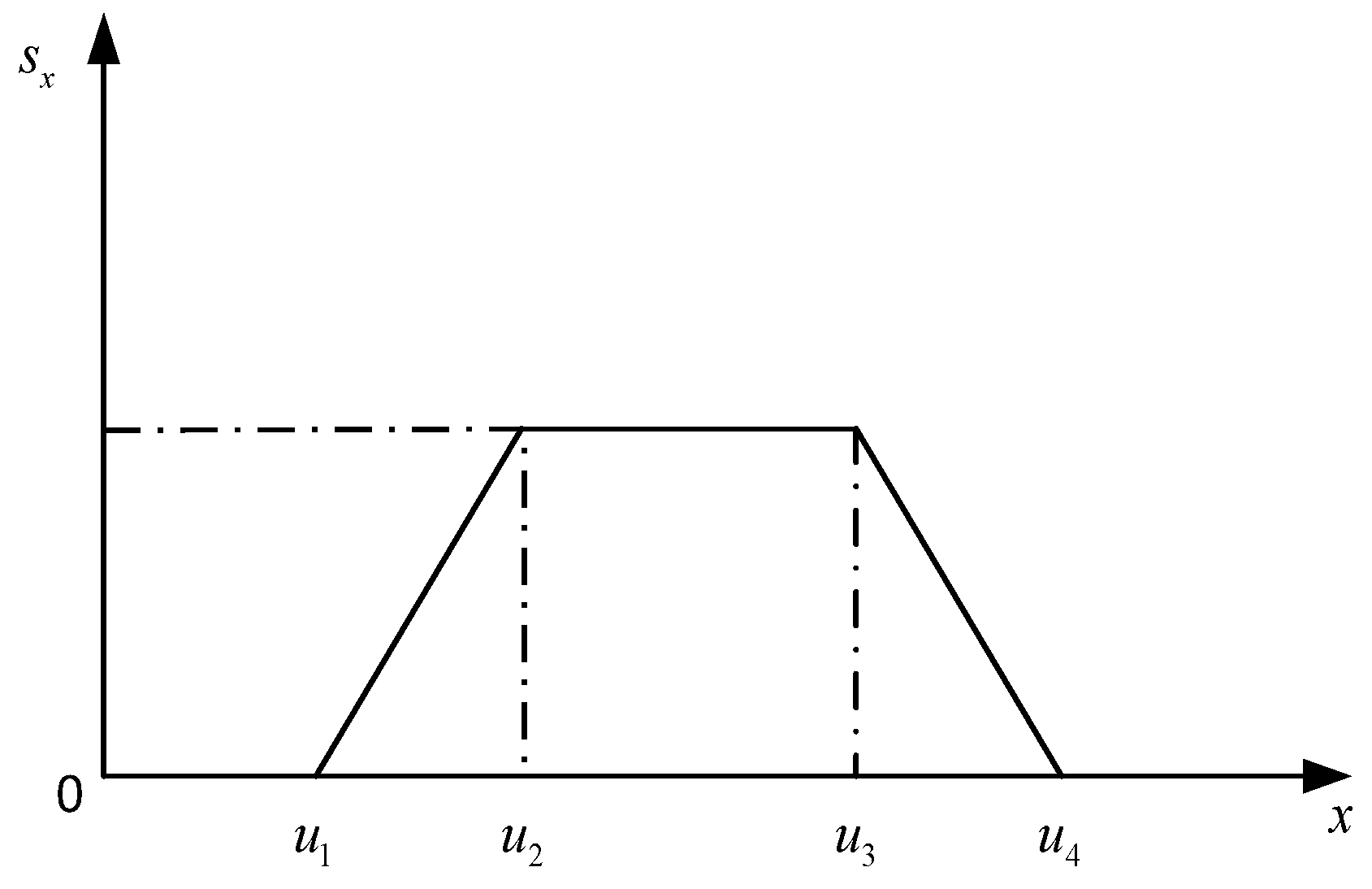
2.2. Intraday Trapezoidal Fuzzy Number Equivalence Model
2.2.1. Trapezoidal Fuzzy Number Expression
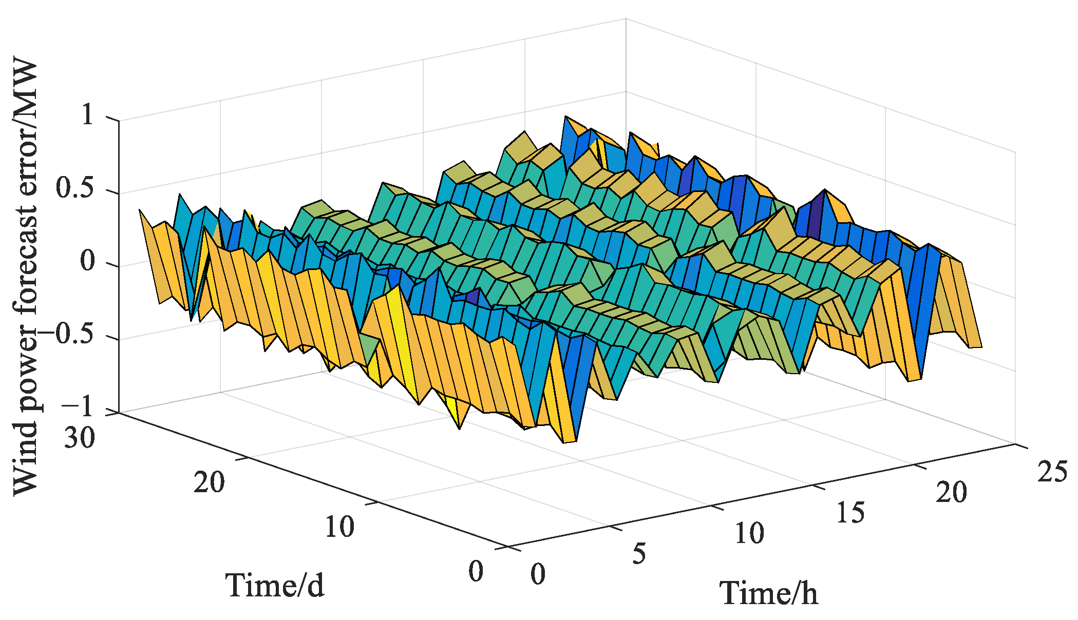
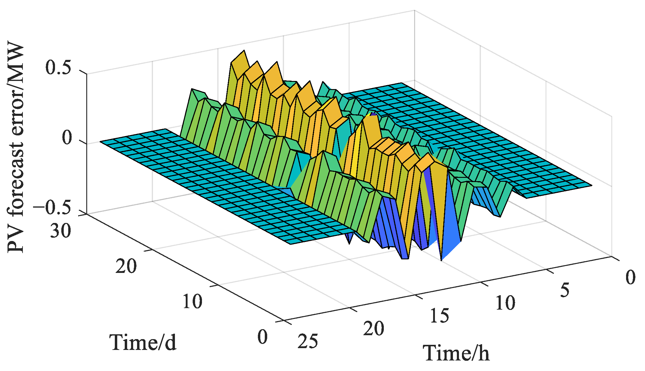
2.2.2. Uncertainty Expression of Wind, PV and Load
3. Scheduling Model of Each Time Scale
3.1. Day-Ahead Scheduling Plan Model
- (1)
- Objective function
- (2)
- Constraints
- Power balance constraints:where is the output of the CSP power station in scenario at time .
- Unit output constraintswhere , are the upper and lower limits of the output of the CSP power station; is the operation state of CSP plant at time , indicates unit operation, indicates unit shutdown; , are the upper and lower limits of the output of the thermal power unit, respectively; , are the upper and lower limits of the output of the wind and solar power plant.
- Unit rotating reserve constraints:where , , and are the positive and negative rotating reserve capacities of the thermal power units and CSP plant, respectively; is the prediction error of the system load; and , is the error rate of load forecasting.
- Ramp rate constraints:where and are the maximum up and down ramp rates of thermal power unit , respectively, and and are the maximum up and down ramp rates of the CSP power plant, respectively.
- Thermal storage system constraints:where is the heat storage capacity of the thermal storage system at time , MW·h; and are the minimum and maximum heat storage capacity of the thermal storage system of the CSP plant; and are the minimum heat charging and discharging power of the thermal storage system at time , respectively; and are the maximum heat charging and discharging power of the thermal storage system at time , respectively; τ is the heat loss coefficient of the thermal storage system.
3.2. Intraday Scheduling Plan Model
- (1)
- Objective function
- (2)
- Constraints
- Power balance constraints:where is the confidence level.
- Units spinning reserve constraints:
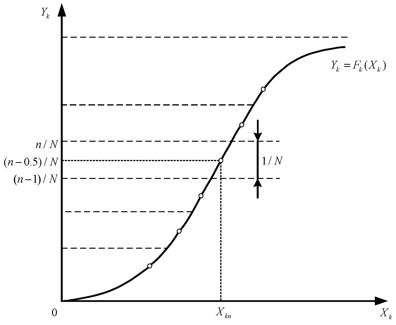
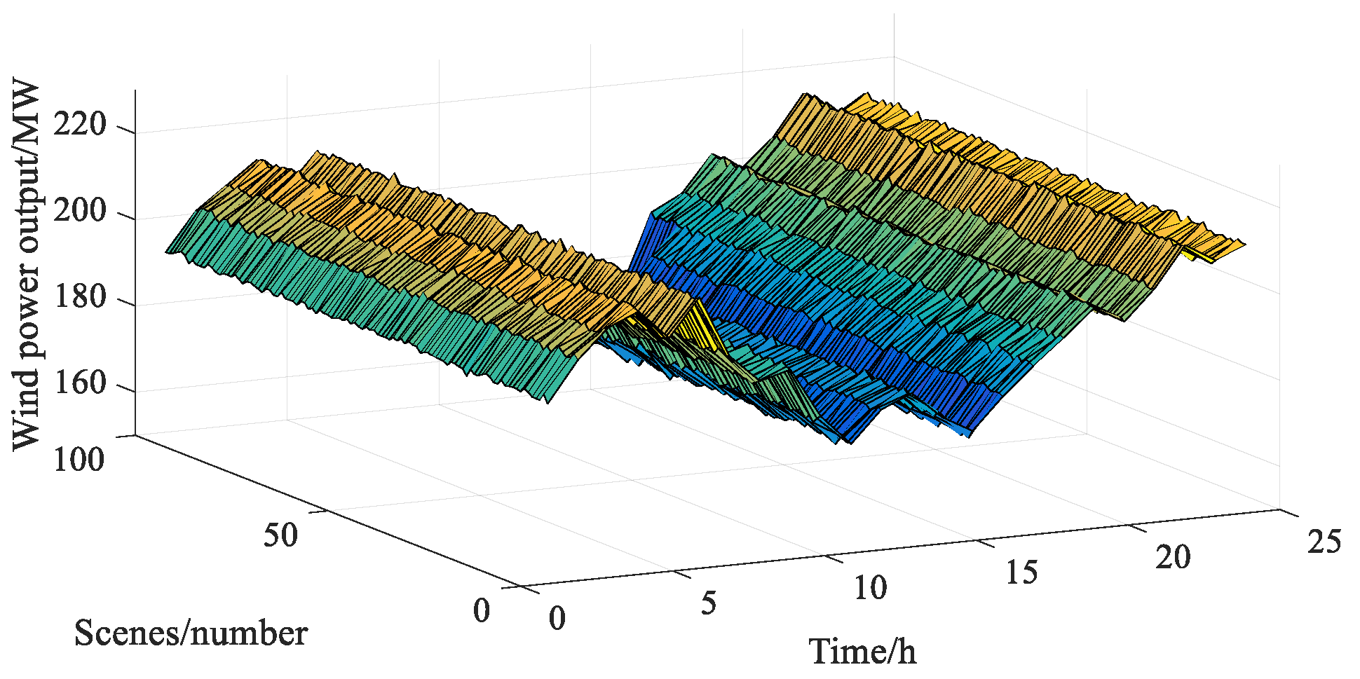
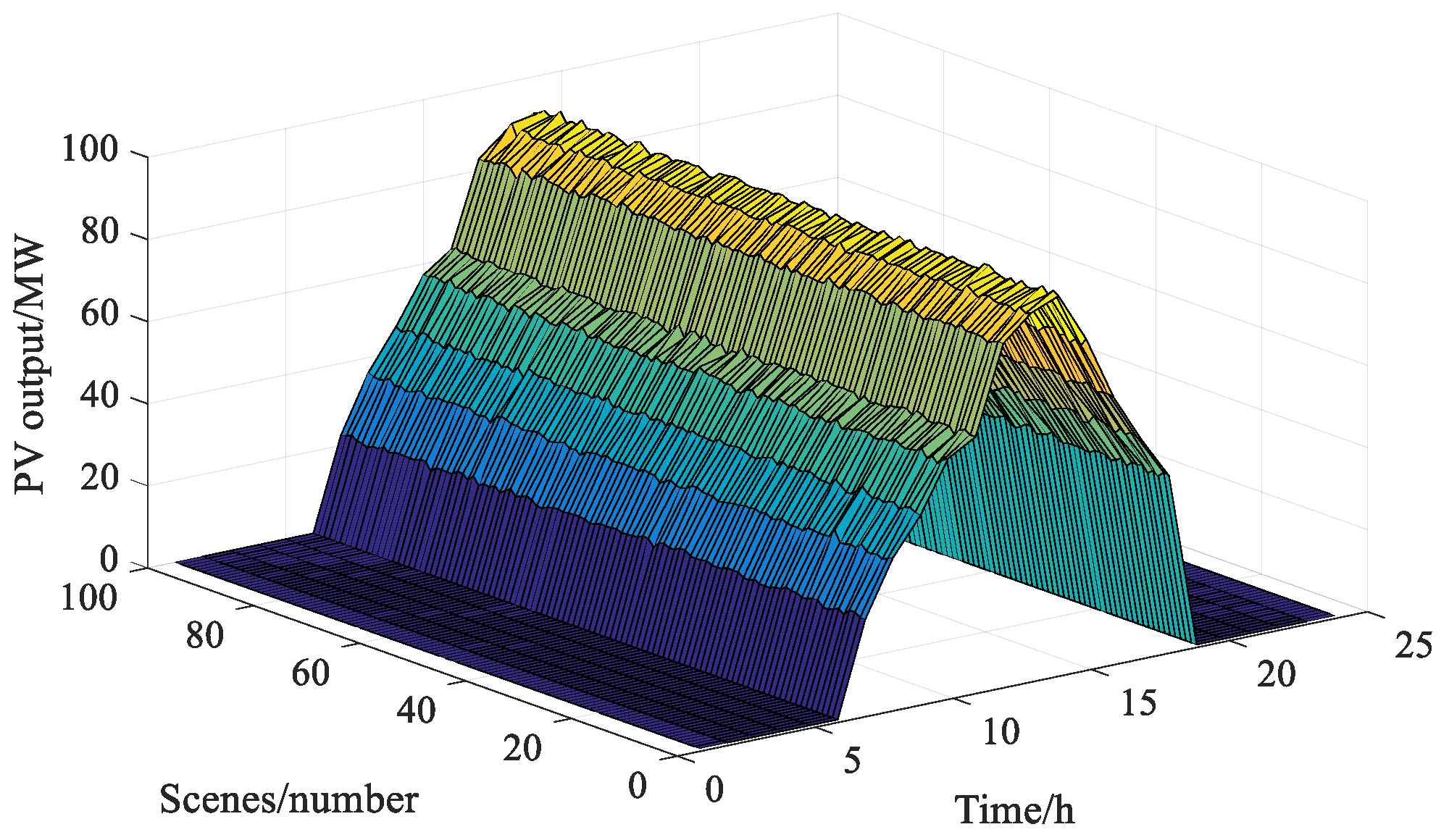
3.3. Scenario Generation and Reduction
3.4. Day-Ahead Multiscene Stochastic Programming Model
- (1)
- Scenario generation
- (2)
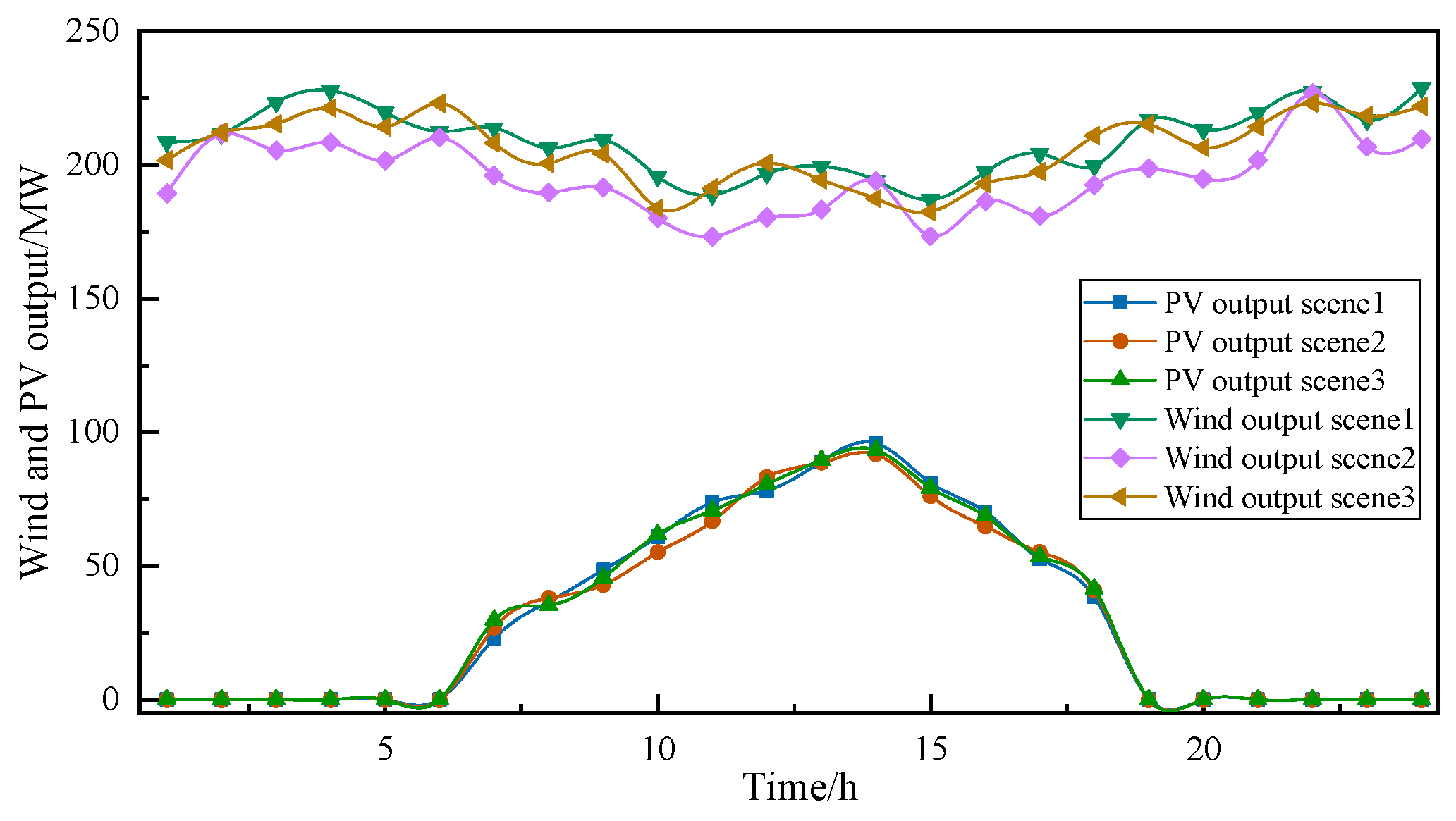
- Scenario reduction
- (3)
- Scenario combination
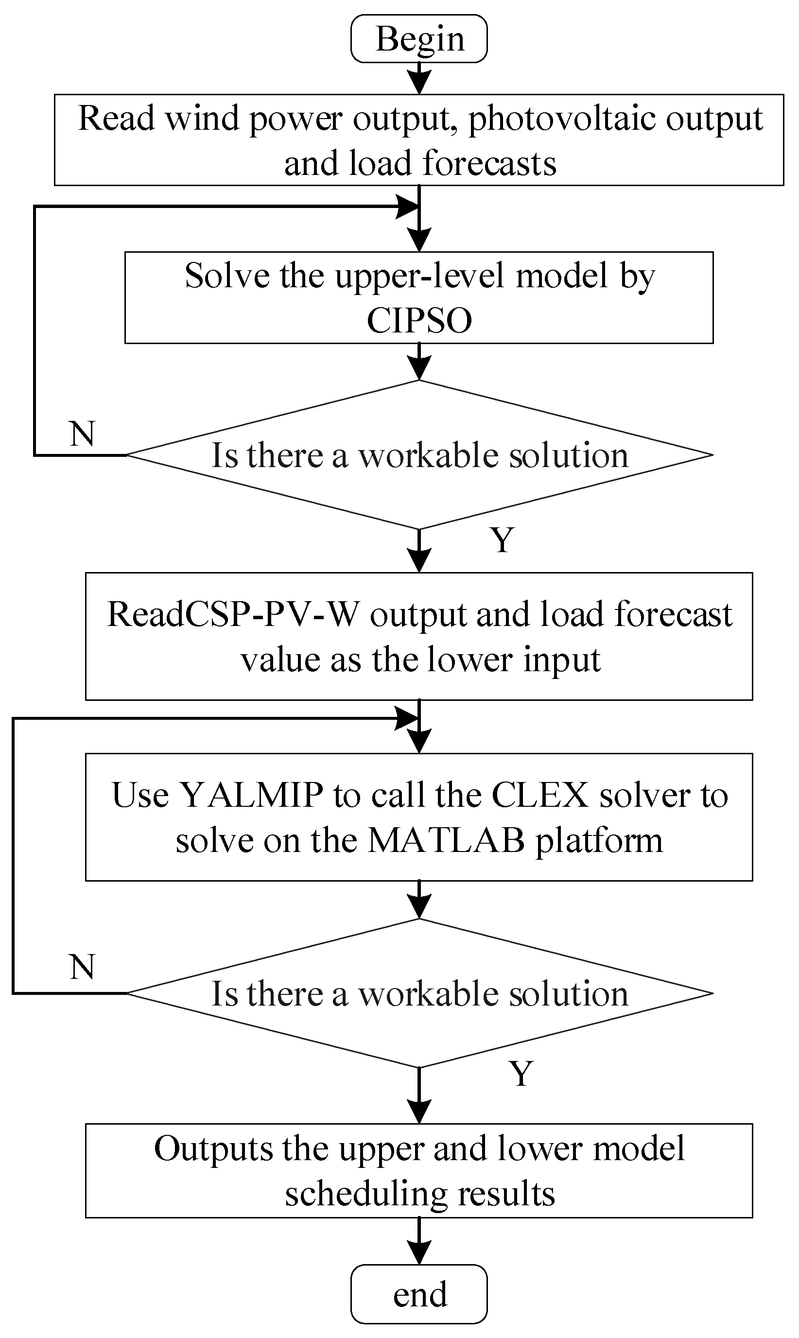
3.5. Model Solving
4. Example Analysis
4.1. Model Solving
4.2. Analysis of Example Results
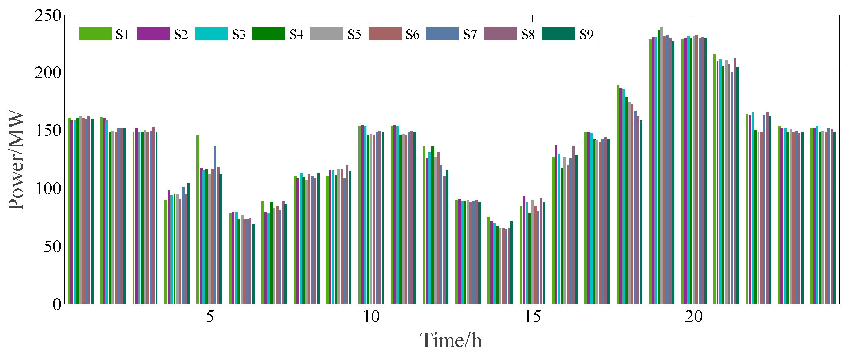
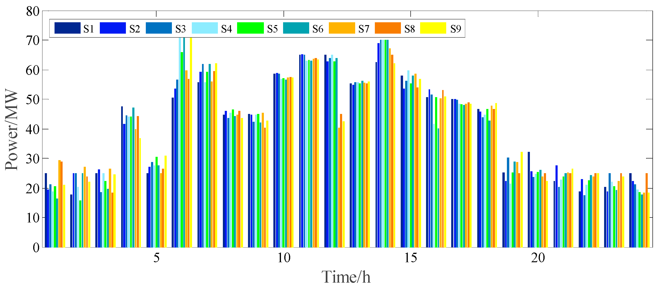
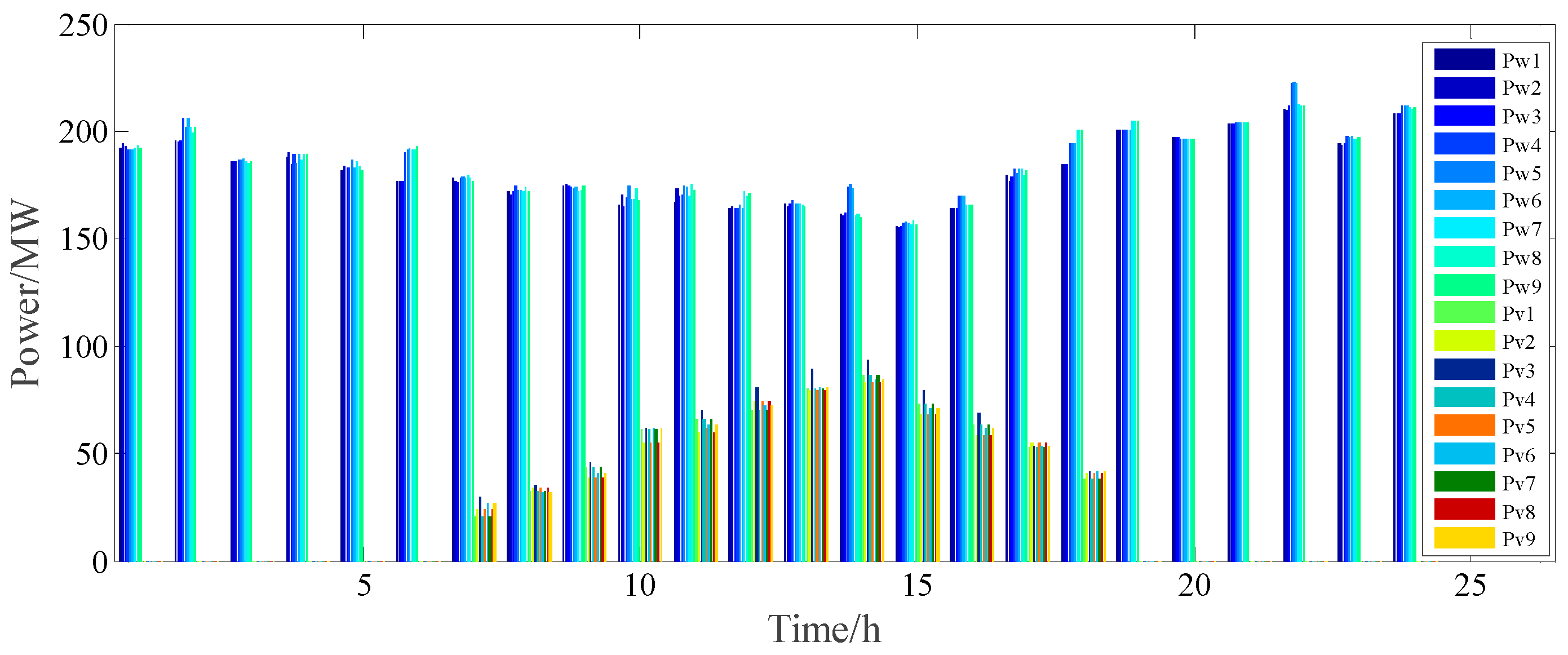
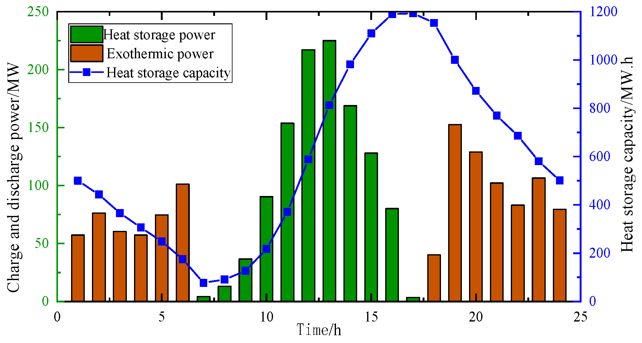
4.2.1. Analysis of Day-Ahead Results
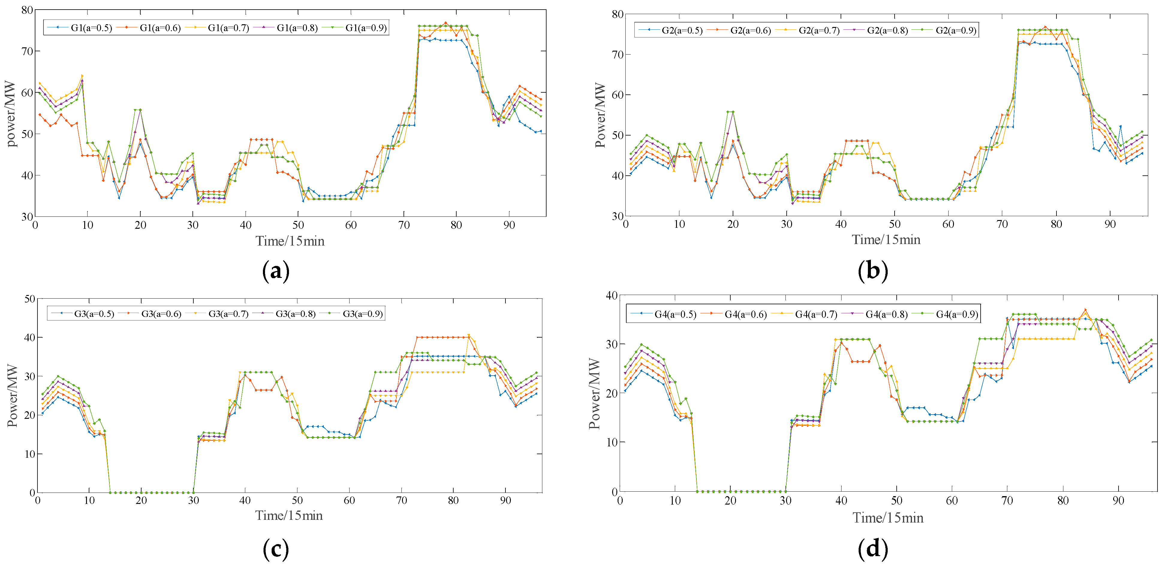
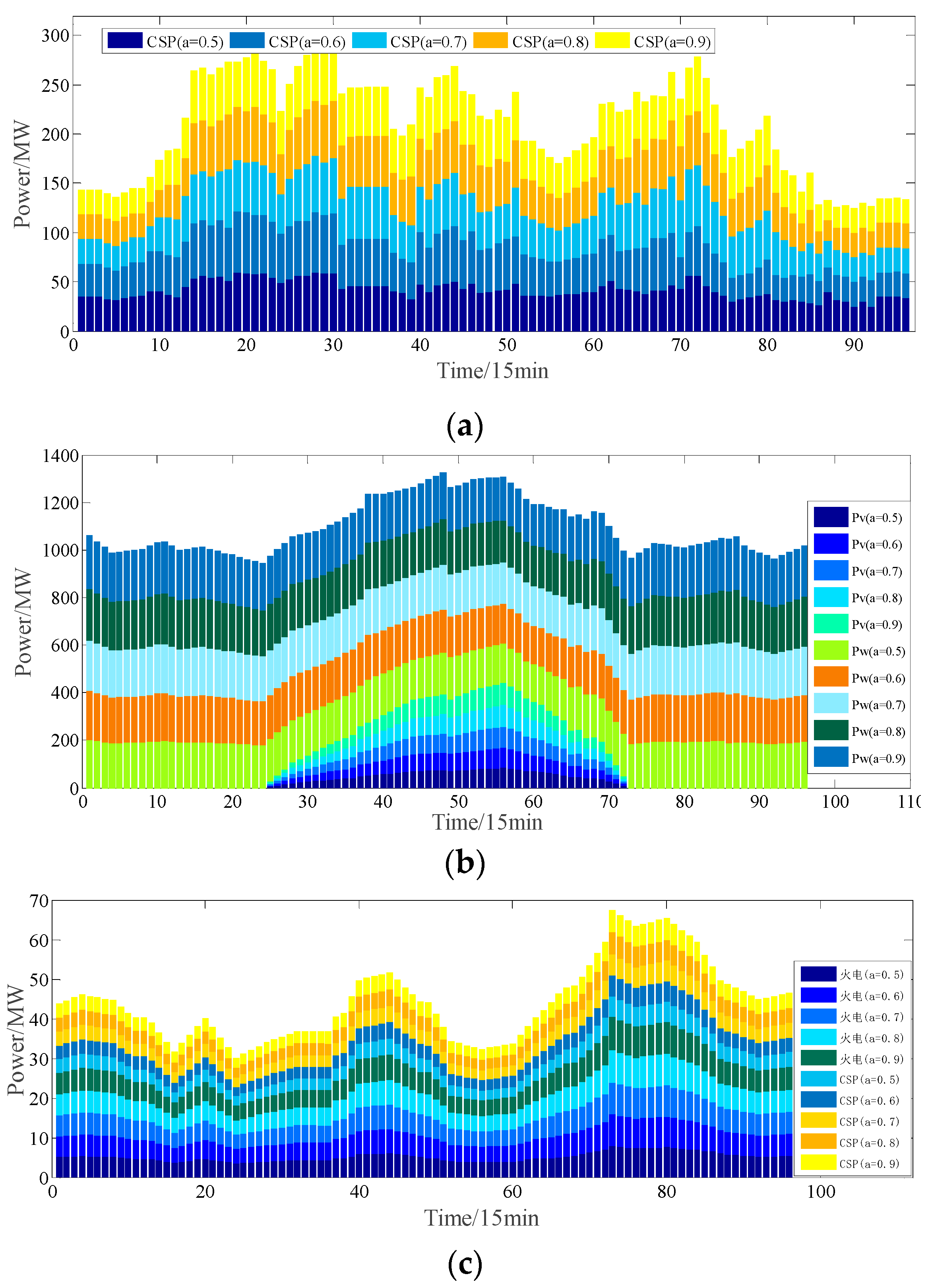
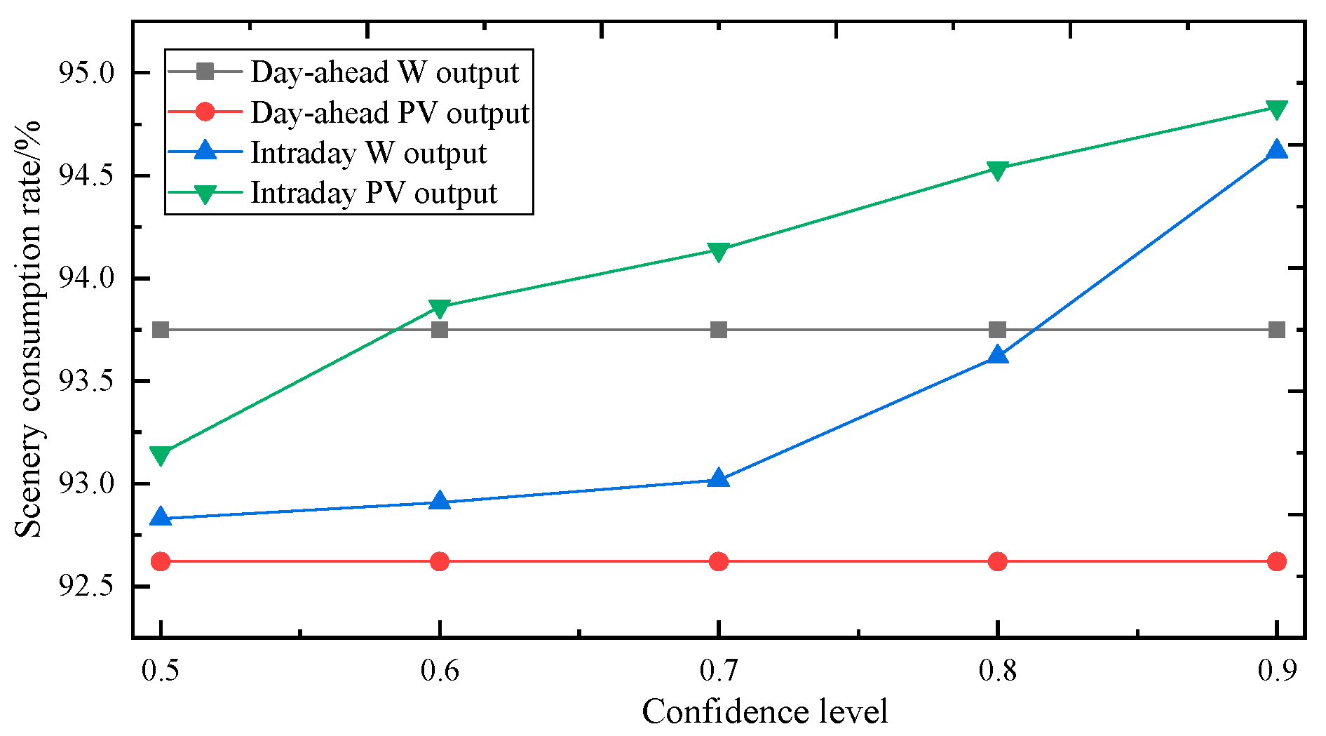
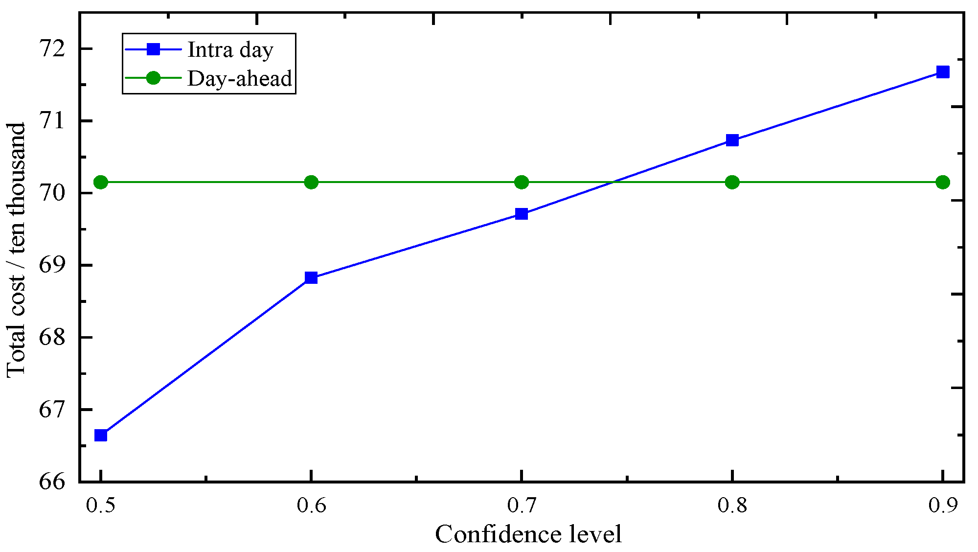
4.2.2. Analysis of Intraday Results
5. Conclusions
- (1)
- A multi-scenario analysis method is used to convert the uncertainty of the day-ahead forecast output of wind and solar energy into a deterministic scenario, and then the fuzzy theory is introduced. The trapezoidal fuzzy number equivalent model is used to characterize the uncertainty of the day-ahead wind and solar energy and load. The example shows that the model can effectively alleviate the problem of a high proportion of new energy-efficient consumption caused by prediction error and wind and solar output fluctuation.
- (2)
- Multiperiod coordinated scheduling can combine more accurate intraday prediction information and make full use of the fast adjustment ability and power shift characteristics of the CSP plants, which can effectively reduce the fluctuation of load after the wind–solar grid connection, thereby reducing the comprehensive operation cost of the system.
Author Contributions
Funding
Data Availability Statement
Conflicts of Interest
Appendix A

| Unit | Upper Limit of Output (MW) | Lower Limit of Output (MW) | Ramp Rate (MW/h) | Fuel Cost | Start-Up and Shut-Down Costs | ||
|---|---|---|---|---|---|---|---|
| a | b | c | H | ||||
| Yuan/MW | Yuan/MW | Yuan/MW | Yuan/MW | ||||
| 1 | 80 | 40 | 40 | 0.02 | 179 | 295 | 1456 |
| 2 | 80 | 40 | 40 | 0.031 | 175 | 350 | 1729 |
| 3 | 50 | 20 | 20 | 0.023 | 100 | 125 | 1982 |
| 4 | 50 | 20 | 20 | 0.015 | 125 | 167 | 2464 |
| Operation Parameters of CSP Plant | Value |
|---|---|
| Rated output power of CSP plant/MW | 100 |
| Minimum output power during operation of CSP plant/MW | 10 |
| Maximum ramp rate of CSP plant/MW/h | 40 |
| Heat loss rate of heat storage system/% | 3 |
| Thermoelectric conversion efficiency of CSP plant/% | 45 |
| Photothermal conversion efficiency of CSP plant/% | 57 |
| Cost coefficient of heating and power generation for collectors/(yuan/MW·h) | 20 |
| Cost coefficient of power generation for heat storage devices/(yuan/MW·h) | 40 |
| Maximum daily heat storage capacity of heat storage system/MW·h | 1000 |
| Initial value of heat storage capacity of heat storage system/MW·h | 600 |
| The lower limit of heat storage system/MW·h | 100 |
| Mirror field area/m | 1.33 × 10⁶ |
| Dissipation coefficient of heat storage system/% | 3.1 |
| Heat storage efficiency of heat storage system/% | 98.5 |
| Heat release efficiency of heat storage system/% | 98.5 |
References
- Zhang, X.; Zhao, C.; Liang, J.; Li, K.; Zhong, J. Robust fuzzy scheduling of power systems considering bilateral uncertainties of generation and demand side. Autom. Electr. Power Syst. 2018, 42, 67–75. [Google Scholar] [CrossRef]
- Wang, H.; Qin, H.; Zhou, C.; Jia, F.; Xu, X.; Pan, X. Cross-regional day-ahead to intra-day scheduling model considering forecasting uncertainty of renewable energy. Autom. Electr. Power Syst. 2019, 43, 60–67. [Google Scholar]
- Jin, H.; Sun, H.; Niu, T.; Guo, Q. Robust unit commitment considering uncertainties of wind and energy intensive load dispatching. Autom. Electr. Power Syst. 2019, 43, 13–20. [Google Scholar] [CrossRef]
- Zhang, J.; Cheng, C.; Shen, J.; Li, G.; Li, X. Short-term Joint Optimal Operation Method for High Proportion Renewable Energy Grid Considering Wind-solar Uncertainty. Proc. Chin. Soc. Elec. Eng. 2020, 40, 5921–5932. [Google Scholar] [CrossRef]
- Yuan, Q.; Wu, Y.; Li, B.; Sun, Y.; Lai, X.; Zhong, H. Multi-timescale coordinated dispatch model and approach considering generation and load uncertainty. Power Syst. Prot. Control 2019, 47, 8–16. [Google Scholar]
- Wang, Q.; Wang, J.; Guan, Y. Stochastic unit commitment with uncertain demand response. IEEE Trans. Power Syst. 2013, 28, 562–563. [Google Scholar] [CrossRef]
- Zhao, C.; Wang, J.; Watson, J.P.; Guan, Y. Multi-stage robust unit commitment considering wind and demand response uncertainties. IEEE Trans. Power Syst. 2012, 28, 2708–2717. [Google Scholar] [CrossRef]
- Yang, S.; Zeng, D.; Ding, H.; Yao, J.; Wang, K. Multi-objective demand response model considering the probabilistic characteristic of price elastic load. Energies 2016, 9, 80. [Google Scholar] [CrossRef]
- Jin, G.; Pan, D.; Chen, Q.; Shi, C.; Li, G. Fuzzy random day-ahead optimal dispatch of dc distribution network considering the uncertainty of source-load. Trans. Chin. Electrotechn. Soc. 2021, 36, 4517–4528. [Google Scholar] [CrossRef]
- Ma, R.; Kang, R.; Jiang, F.; Xiong, L.; Li, L.; Xu, H. Multi-objective dispatch planning of power system considering the stochastic and fuzzy wind power. Power Syst. Prot. Control 2013, 41, 150–156. [Google Scholar]
- Cui, Y.; Li, C.; Zhao, Y.; Zhong, W.; Wang, M. Source-grid-load multi-time interval optimization scheduling method considering wind-photovoltaic-photothermal combined DC transmission. Proc. Chin. Soc. Elec. Eng. 2022, 42, 559–573. [Google Scholar] [CrossRef]
- Xiong, H.; Xiang, T.; Chen, H.; Lin, F.; Su, J. Research of fuzzy chance constrained unit commitment containing large-scale intermittent power. Proc. Chin. Soc. for Elec. Eng. 2013, 33, 36–44. [Google Scholar] [CrossRef]
- Zhao, D.; Yin, J. Fuzzy random chance constrained preemptive goal programming scheduling model considering source-side and load-side uncertainty. Trans. Chin. Electrotech. Soc. 2018, 33, 1076–1185. [Google Scholar] [CrossRef]
- Li, W.; Zhou, J.; Xie, K.; Xiong, X. Power system risk assessment using a hybrid method of fuzzy set and Monte Carlo simulation. IEEE Trans. Power Syst. 2008, 23, 336–343. [Google Scholar] [CrossRef]
- Li, G.; Li, X.; Bian, J.; Li, Z. Two level scheduling strategy for inter-provincial dc power grid considering the uncertainty of PV-load prediction. Proc. Chin. Soc. Elec. Eng. 2021, 41, 4763–4776. [Google Scholar] [CrossRef]
- Zhong, W.; Huang, S.; Cui, Y.; Xu, J.; Zhao, Y. W-S-C Capture coordination in virtual power plant considering source-load uncertainty. Power Syst. Technol. 2020, 44, 3424–3432. [Google Scholar] [CrossRef]
- Jiang, Z.; Li, s.; Ma, X.; Li, X.; Kang, Y.; Li, H.; Dong, H. State estimation of regional power systems with source-load two-terminal uncertainties. Comp. Model. Eng. 2022, 132, 295–317. [Google Scholar] [CrossRef]
- Li, Z.; Zhang, Z. Day-ahead and intra-day optimal scheduling of integrated energy system considering uncertainty of source & load power forecasting. Energies 2021, 14, 2539. [Google Scholar] [CrossRef]
- Chen, R.; Sun, H.; Li, Z.; Liu, Y. Grid dispatch model and interconnection benefit analysis of concentrating solar power plants with thermal storage. Autom. Electr. Power Syst. 2014, 38, 1–7. [Google Scholar] [CrossRef]
- Cui, Y.; Yang, Z.; Zhang, J.; Wang, M.; Yan, G. Scheduling strategy of wind power-photovoltaic power-concentrating solar power considering comprehensive costs. High Vol. Eng. 2019, 45, 269–275. [Google Scholar]


| Scenarios | Combined Scene Probability % | Wind Power Consumption Rate % | PV Power Consumption Rate % |
|---|---|---|---|
| S1 | 11.25 | 94.0 | 91.2 |
| S2 | 7.5 | 94.6 | 97.6 |
| S3 | 6.25 | 93.8 | 94.3 |
| S4 | 15.75 | 94.1 | 92.3 |
| S5 | 10.5 | 93.9 | 92.8 |
| S6 | 8.75 | 94.5 | 93.1 |
| S7 | 18 | 92.6 | 92.3 |
| S8 | 12 | 95.3 | 91.8 |
| S9 | 10 | 93.9 | 90.9 |
| Scenarios | Comprehensive Cost/Million Yuan | Combined Scene Probability % | Comprehensive Cost after Multiplying Probability Million Yuan |
|---|---|---|---|
| S1 | 70.561 | 11.25 | 7.938 |
| S2 | 70.916 | 7.5 | 5.318 |
| S3 | 71.618 | 6.25 | 4.476 |
| S4 | 69.402 | 15.75 | 10.93 |
| S5 | 69.807 | 10.5 | 7.329 |
| S6 | 69.618 | 8.75 | 6.091 |
| S7 | 69.887 | 18 | 12.579 |
| S8 | 69.572 | 12 | 8.348 |
| S9 | 69.971 | 10 | 6.997 |
| Confidence Level | Comprehensive Operation Cost Million Yuan | Wind Power Consumption Rate % | PV Power Consumption Rate % |
|---|---|---|---|
| a = 0.5 | 66.646 | 92.83 | 93.14 |
| a = 0.6 | 68.825 | 92.92 | 93.86 |
| a = 0.7 | 69.711 | 93.01 | 94.14 |
| a = 0.8 | 70.732 | 93.61 | 94.53 |
| a = 0.9 | 71.676 | 94.66 | 94.86 |
Disclaimer/Publisher’s Note: The statements, opinions and data contained in all publications are solely those of the individual author(s) and contributor(s) and not of MDPI and/or the editor(s). MDPI and/or the editor(s) disclaim responsibility for any injury to people or property resulting from any ideas, methods, instructions or products referred to in the content. |
© 2023 by the authors. Licensee MDPI, Basel, Switzerland. This article is an open access article distributed under the terms and conditions of the Creative Commons Attribution (CC BY) license (https://creativecommons.org/licenses/by/4.0/).
Share and Cite
Xu, M.; Li, W.; Feng, Z.; Bai, W.; Jia, L.; Wei, Z. Economic Dispatch Model of High Proportional New Energy Grid-Connected Consumption Considering Source Load Uncertainty. Energies 2023, 16, 1696. https://doi.org/10.3390/en16041696
Xu M, Li W, Feng Z, Bai W, Jia L, Wei Z. Economic Dispatch Model of High Proportional New Energy Grid-Connected Consumption Considering Source Load Uncertainty. Energies. 2023; 16(4):1696. https://doi.org/10.3390/en16041696
Chicago/Turabian StyleXu, Min, Wanwei Li, Zhihui Feng, Wangwang Bai, Lingling Jia, and Zhanhong Wei. 2023. "Economic Dispatch Model of High Proportional New Energy Grid-Connected Consumption Considering Source Load Uncertainty" Energies 16, no. 4: 1696. https://doi.org/10.3390/en16041696