
Modular and Transferable Machine Learning for Heat Management and Reuse in Edge Data Centers

Abstract
:1. Introduction
Related Work
2. Materials
2.1. Fan Control Board
2.2. Data Collection
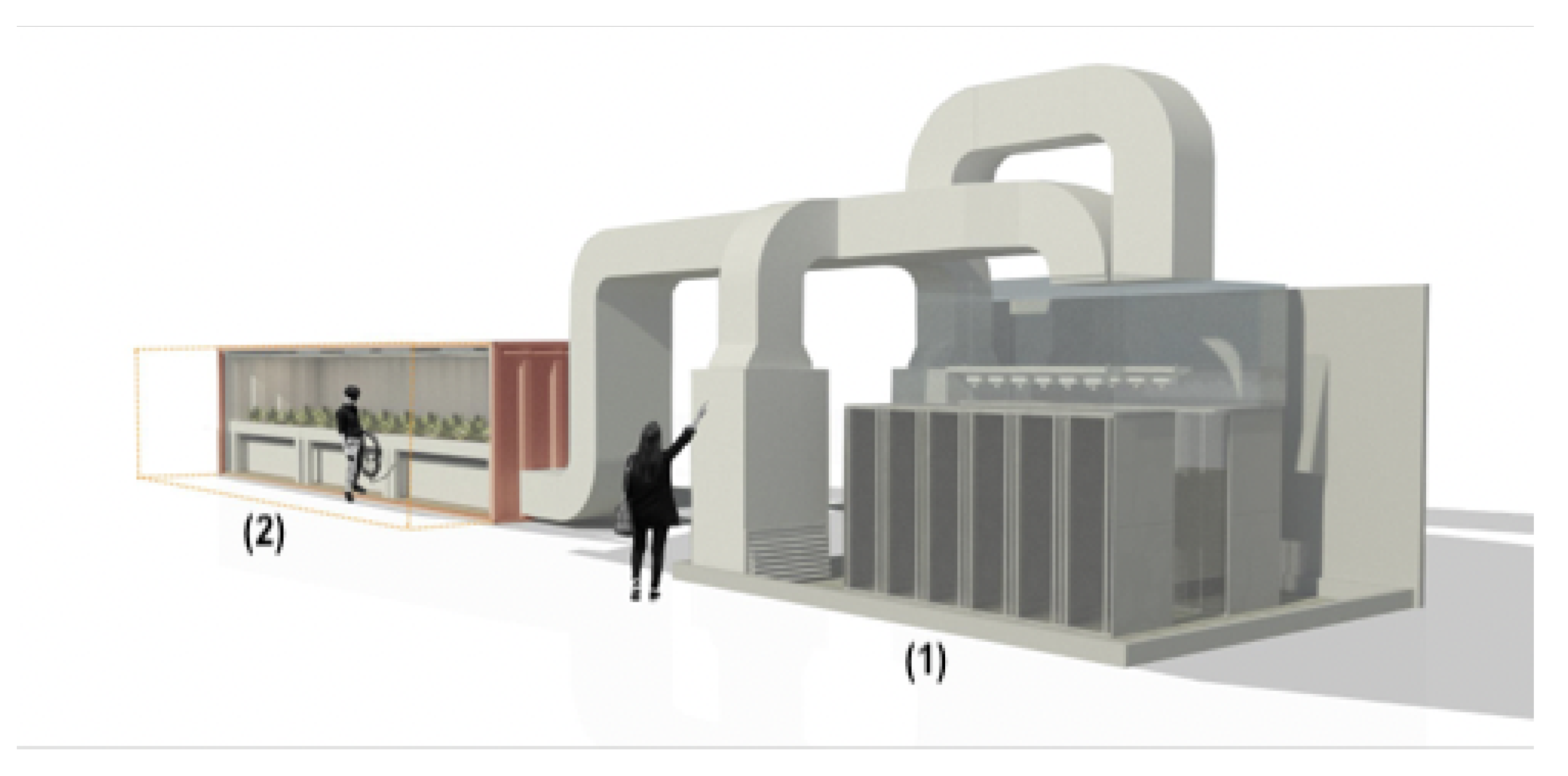
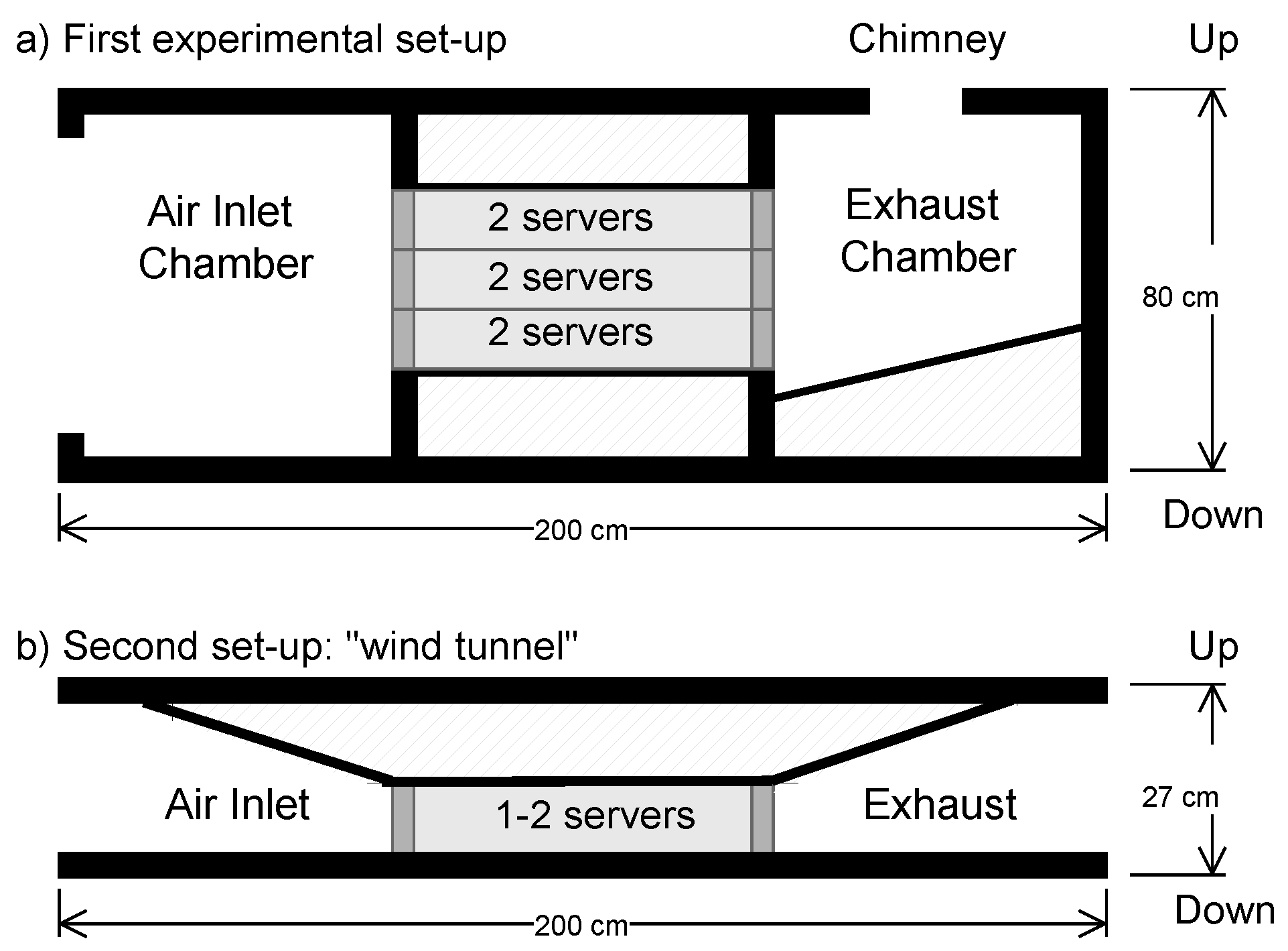
2.3. Experiment Design
3. Method
3.1. Notation
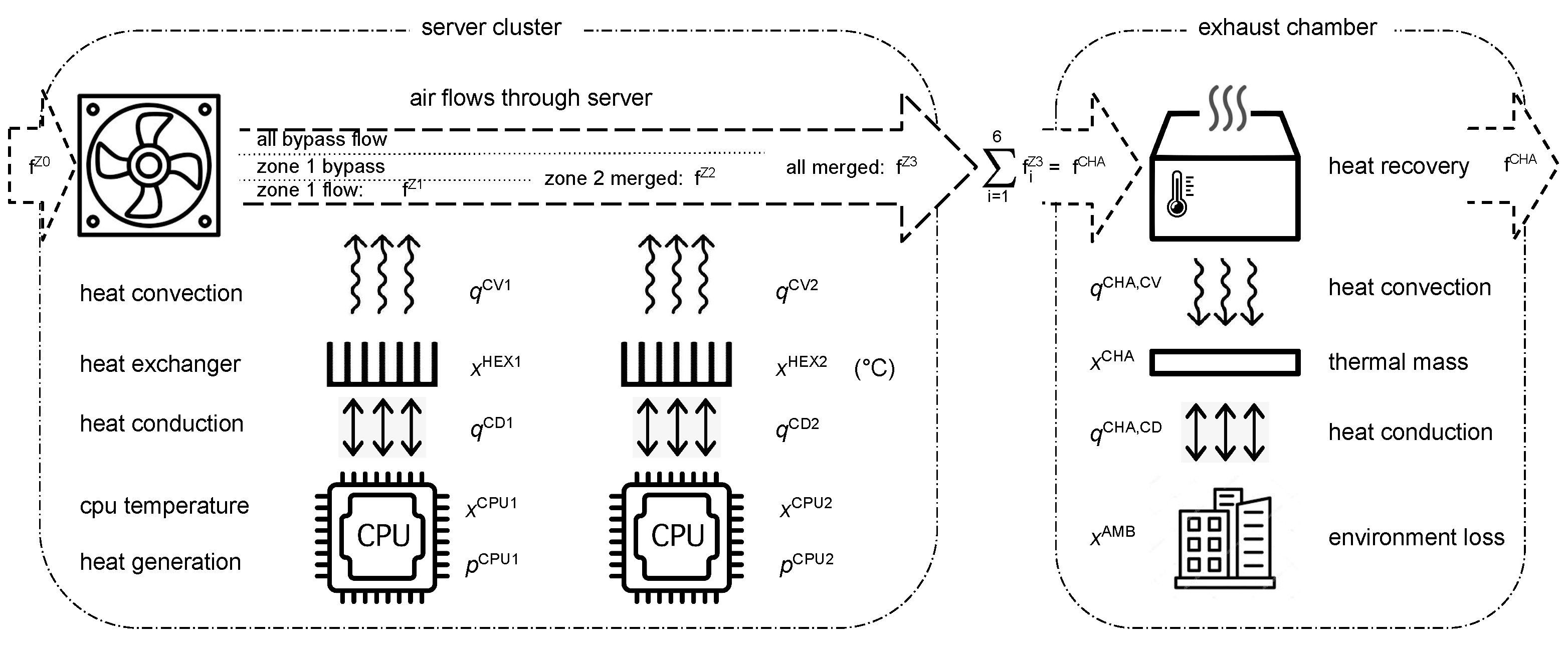
3.2. Thermal Model
- Conductive heat transfer only occurs between a CPU and its heat sink;
- Only heat sinks are affected by convection of the cooling air-flow .
3.3. Physics-Informed Data-Driven RNN
3.4. Alternative Models
3.5. n-Step PEM
3.6. Regularization
4. Results
4.1. Model Training
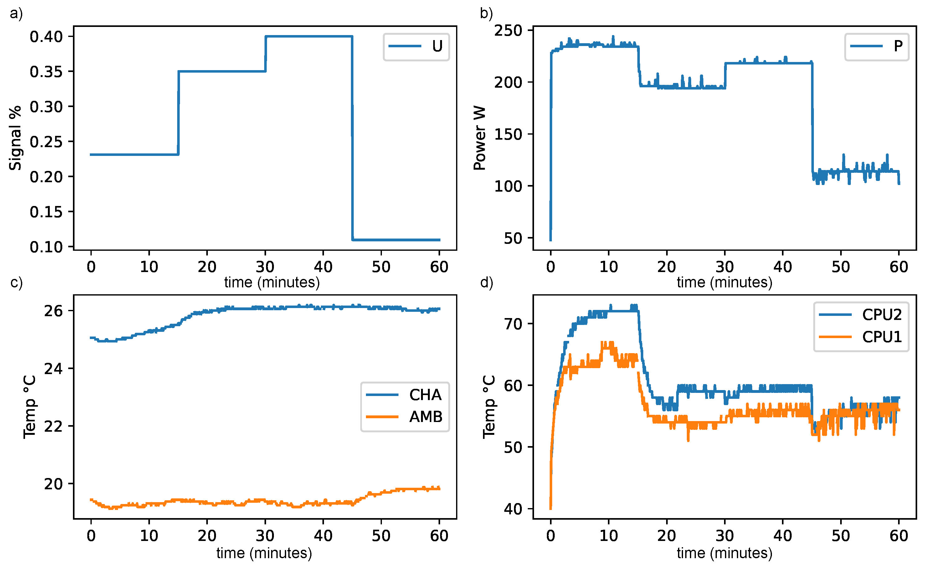
4.2. Fan Control
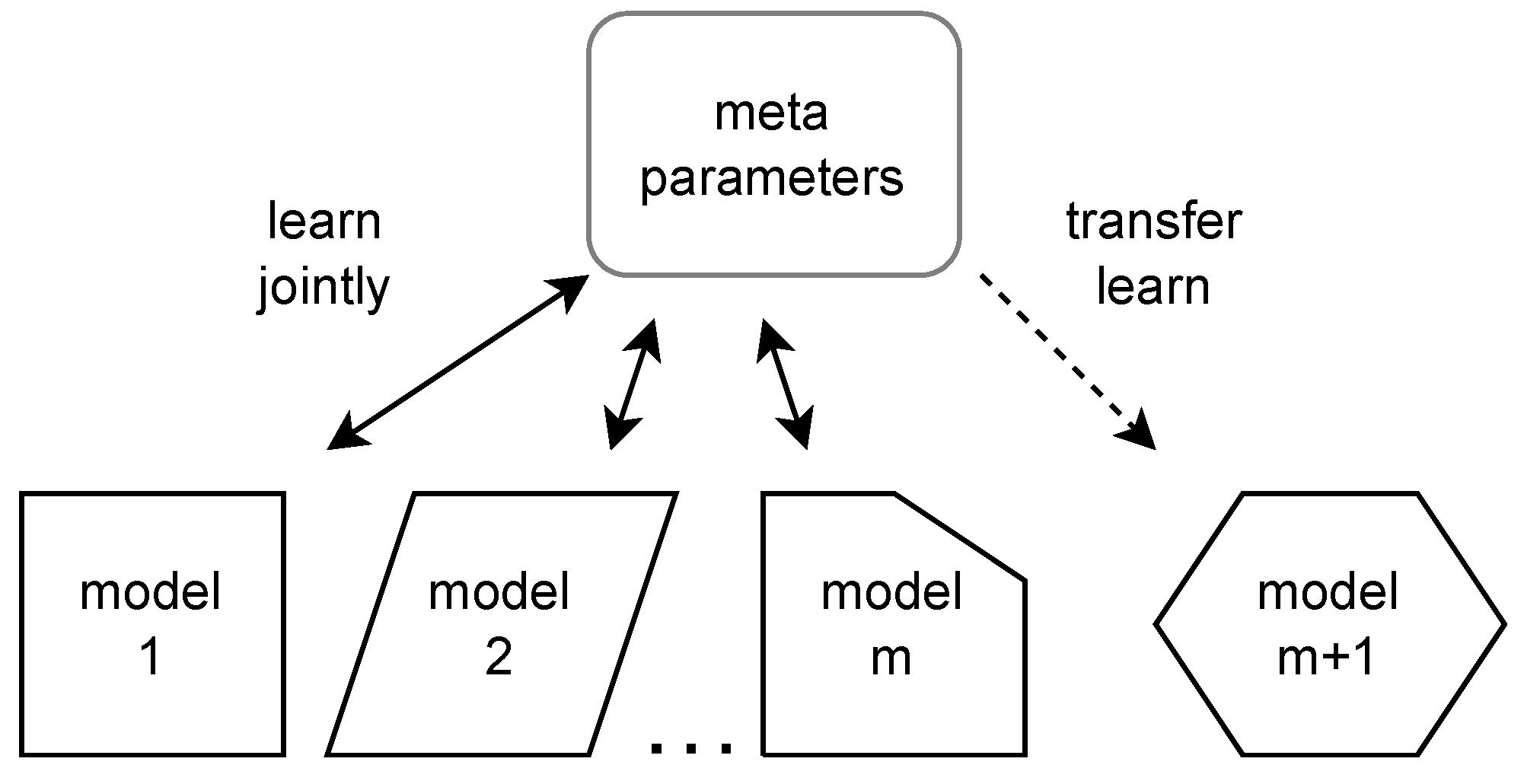
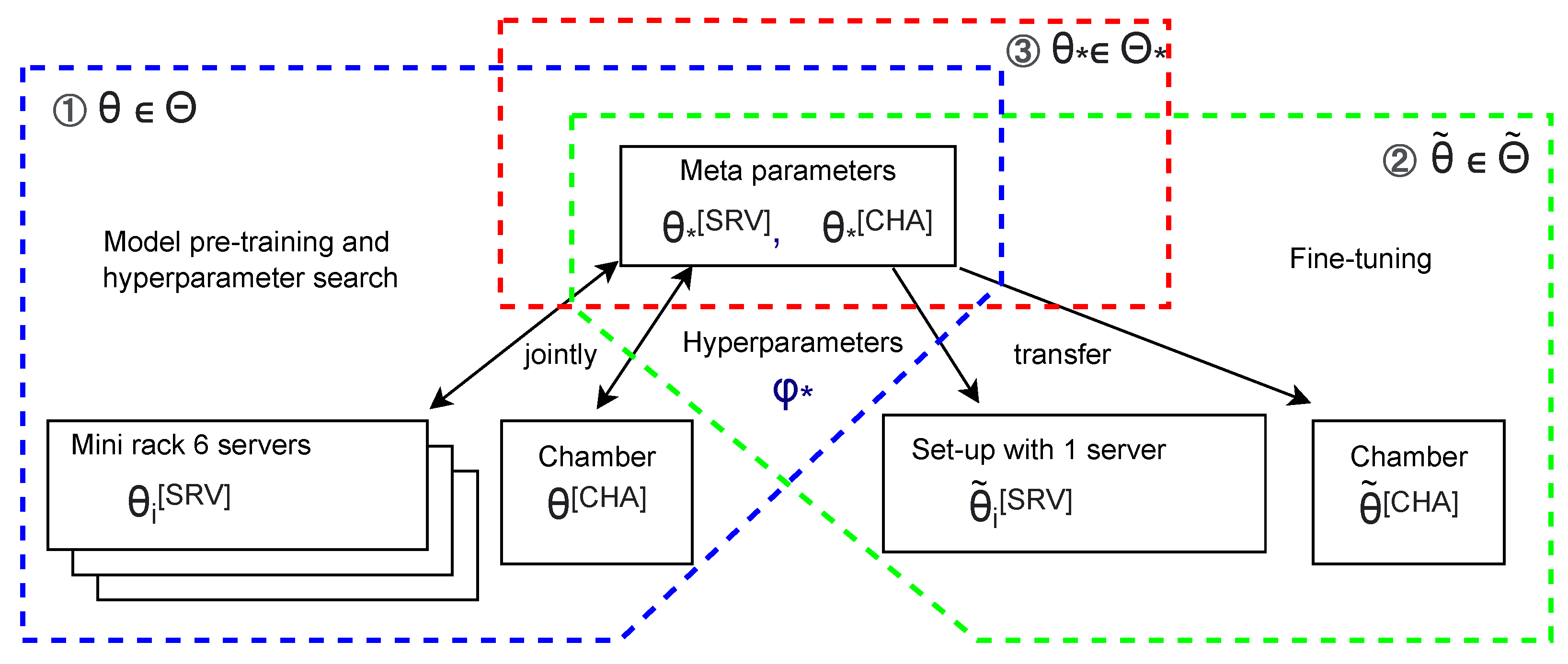
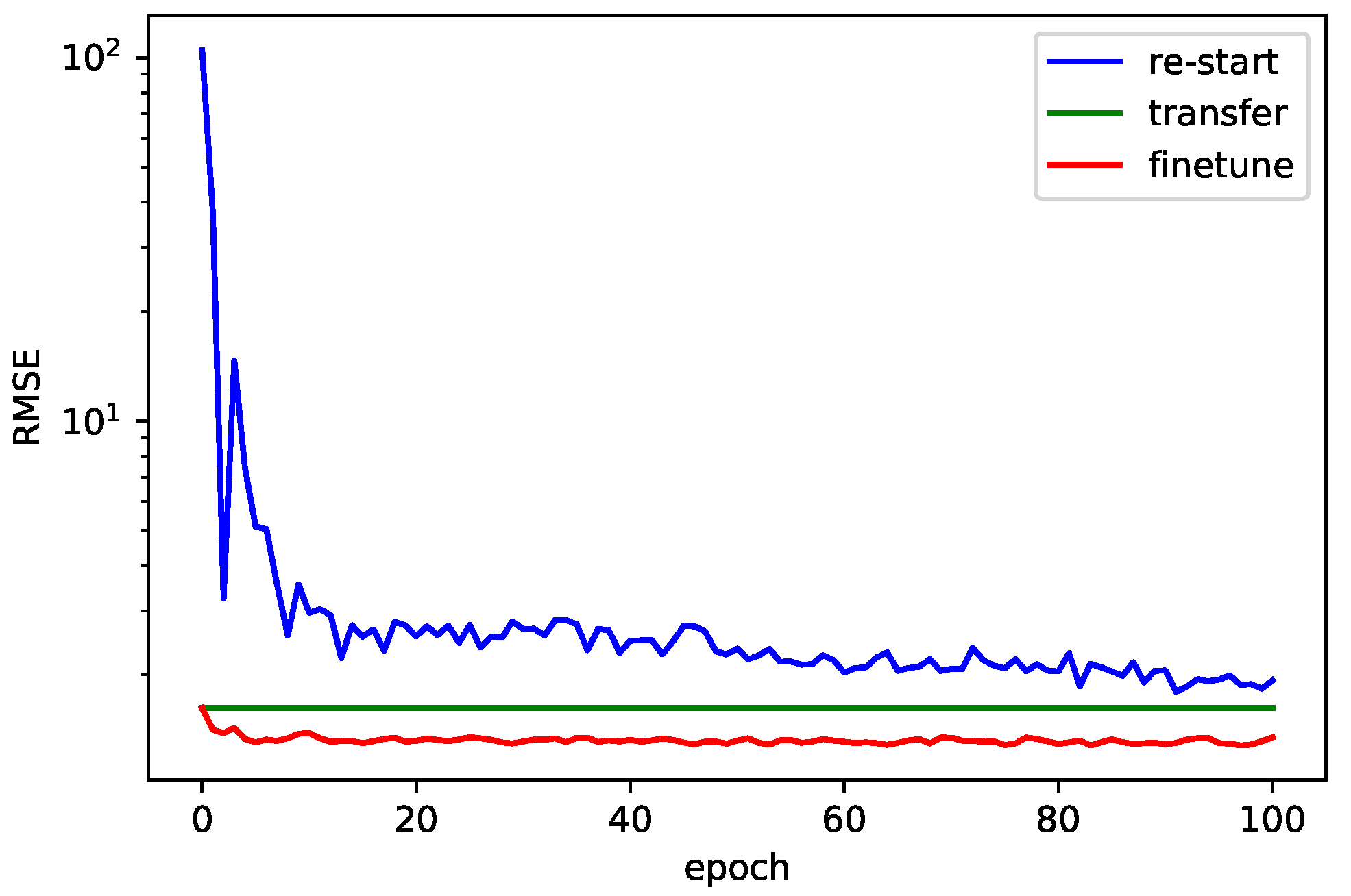
4.3. Transfer Learning
5. Discussion
6. Conclusions
Author Contributions
Funding
Institutional Review Board Statement
Informed Consent Statement
Conflicts of Interest
Abbreviations and Notation
| CFD | Computational Fluid Dynamics |
| DC | Data Center |
| MPC | Model Predictive Control |
| MSE | Mean Square Error |
| MAE | Mean Average Error |
| OCP | Open Compute Project |
| PEM | Prediction Error Minimization |
| PWM | Pulse Width Modulation |
| PID | Proportional-Integral-Derivative |
| PIDD | Physical Informed Data Driven |
| RHC | Receding Horizon Control |
| RMSE | Root Mean Square Error |
| RNN | Recurrent Neural Network |
| SSM | State Space Model |
| ReLU | Rectified Linear Unit (activation function) |
| Hub | Huber (loss function) |
| AMB | ambient (in experiments) |
| CHA | chamber (in experiments) |
| CPU1 | 1st CPU (in experiments) |
| CPU2 | 2nd CPU (in experiments) |
| HEX1 | heat exchanger 1 (in experiments) |
| HEX2 | heat exchanger 2 (in experiments) |
| SRV | server (in experiments) |
| Ambient temperature at time t | |
| Temperature of CPU 1 for server i at time t | |
| Power input through CPU 1 for server i at time t | |
| Temperature of heat exchanger of CPU 1 for server i at time t | |
| Conductive heat transfer in zone 1 server i at time t | |
| Convective heat transfer in zone 1 server i at time t | |
| Temperature of air that enter zone 1 of server i at time t | |
| Temperature of air that exit zone 1 of server i at time t | |
| Mass (air) flow in zone 1 server i at time t | |
| Convective thermal resistance in zone 1 of server i at time t | |
| Temperature of air entering exhaust chamber at time t | |
| Temperature of lump mass of exhaust chamber at time t | |
| Conductive heat transfer in chamber at time t | |
| Convective heat transfer in chamber at time t | |
| Trainable parameter for lump thermal capacitance (CPU 1) | |
| Trainable parameter for conductive thermal resistance (zone 1) | |
| Trainable regression intercept parameter for fan airflow for server i | |
| Trainable regression slope parameter for fan airflow for server i | |
| Trainable regression intercept parameter for zone 1 airflow for server i | |
| Trainable regression slope parameter for zone 1 airflow for server i | |
| Trainable parameter for lump thermal capacitance of chamber | |
| Steady state input power for CPU 1 | |
| Steady state flow heat for zone 1 of server i | |
| Steady state temperature of CPU 1 of server i | |
| Steady state temperature for heat exchanger 1 of server i | |
| Parameter that control the relative weight of chamber set-point | |
| Parameter for the length of the model predictive control horizon | |
| Penalty parameter for signal strength | |
| Penalty parameter for signal smoothness | |
| Penalty parameter for signal heterogeneity | |
| Hyper-parameter for strength of hierarchical regularization | |
| Hyper-parameter for strength of noise smoothing | |
| n | Hyper-parameter for length of prediction window |
| r | Hyper-parameter for learning rate |
| K | Hyper-parameter for number of training epochs |
Appendix A. Model Details
Appendix A.1. Server Model
Appendix A.2. Chamber Model
References
- Khalaj, A.; Halgamuge, S.K. A Review on efficient thermal management of air- and liquid-cooled data centers: From chip to the cooling system. Appl. Energy 2017, 205, 1165–1188. [Google Scholar] [CrossRef]
- Athavale, J.; Yoda, M.; Joshi, Y. Comparison of data driven modeling approaches for temperature prediction in data centers. Int. J. Heat Mass Transf. 2019, 135, 1039–1052. [Google Scholar] [CrossRef]
- Manaserh, Y.M.; Tradat, M.I.; Bani-Hani, D.; Alfallah, A.; Sammakia, B.G.; Nemati, K.; Seymour, M.J. Machine learning assisted development of IT equipment compact models for data centers energy planning. Appl. Energy 2022, 305, 117846. [Google Scholar] [CrossRef]
- Wang, Z.; Bash, C.; Tolia, N.; Marwah, M.; Zhu, X.; Ranganathan, P. Optimal fan speed control for thermal management of servers. In Proceedings of the ASME InterPack Conference 2009, IPACK2009, San Francisco, CA, USA, 19–23 July 2009; Volume 2, pp. 709–719. [Google Scholar]
- Han, X.; Joshi, Y. Energy reduction in server cooling via real time thermal control. In Proceedings of the Annual IEEE Semiconductor Thermal Measurement and Management Symposium, San Jose, CA, USA, 18–22 March 2012; pp. 74–81. [Google Scholar]
- Wang, X.; Liu, Y.; Tian, T.; Li, J. Directly air-cooled compact looped heat pipe module for high power servers with extremely low power usage effectiveness. Appl. Energy 2022, 319, 119279. [Google Scholar] [CrossRef]
- Li, J.; Zhou, G.; Tian, T.; Li, X. A new cooling strategy for edge computing servers using compact looped heat pipe. Appl. Therm. Eng. 2021, 187, 116599. [Google Scholar] [CrossRef]
- Iyengar, M.; Hamann, H.; Schmidt, R.R.; Vangilder, J. Comparison between numerical and experimental temperature distributions in a small data center test cell. In Proceedings of the 2007 ASME InterPack Conference, IPACK 2007, Vancouver, BC, Canada, 8–12 July 2007; Volume 1, pp. 819–826.
- Wibron, E.; Ljung, A.L.; Lundström, T. Computational Fluid Dynamics Modeling and Validating Experiments of Airflow in a Data Center. Energies 2018, 11, 644. [Google Scholar] [CrossRef] [Green Version]
- Pardey, Z.; Demetriou, D.; Erden, H.; VanGilder, J.; Khalifa, H.; Schmidt, R. Proposal for standard compact server model for transient data center simulations. Ashrae Trans. 2015, 121, 413–421. [Google Scholar]
- VanGilder, J.; Healey, C.; Pardey, Z.; Zhang, X. A compact server model for transient data center simulations. Ashrae Trans. 2013, 119, 358–370. [Google Scholar]
- Erden, H.; Ezzat Khalifa, H.; Schmidt, R. Transient thermal response of servers through air temperature measurements. In Proceedings of the International Electronic Packaging Technical Conference and Exhibition, Burlingame, CA, USA, 16–18 July 2013; Volume 2. [Google Scholar] [CrossRef]
- Lucchese, R.; Olsson, J.; Ljung, A.L.; Garcia-Gabin, W.; Varagnolo, D. Energy savings in data centers: A framework for modelling and control of servers’ cooling. IFAC-PapersOnLine 2017, 50, 9050–9057. [Google Scholar] [CrossRef]
- Eriksson, M.; Lucchese, R.; Gustafsson, J.; Ljung, A.L.; Mousavi, A.; Varagnolo, D. Monitoring and modelling open compute servers. In Proceedings of the IECON 2017—43rd Annual Conference of the IEEE Industrial Electronics Society, Beijing, China, 29 October–1 November 2017; pp. 7177–7184. [Google Scholar]
- Open Compute Project. 2019. Available online: https://www.opencompute.org/about (accessed on 25 February 2023).
- VanGilder, J.W.; Healey, C.M.; Condor, M.; Tian, W.; Menusier, Q. A Compact Cooling-System Model for Transient Data Center Simulations. In Proceedings of the 2018 17th IEEE Intersociety Conference on Thermal and Thermomechanical Phenomena in Electronic Systems (ITherm), San Diego, CA, USA, 29 May–1 June 2018. [Google Scholar] [CrossRef]
- Healey, C.; VanGilder, J.; Condor, M.; Tian, W. Transient Data Center Temperatures after a Primary Power Outage. In Proceedings of the 2018 17th IEEE Intersociety Conference on Thermal and Thermomechanical Phenomena in Electronic Systems (ITherm), San Diego, CA, USA, 29 May–1 June 2018; pp. 865–870. [Google Scholar] [CrossRef]
- Lucchese, R.; Johansson, A. On energy efficient flow provisioning in air-cooled data servers. Control. Eng. Pract. 2019, 89, 103–112. [Google Scholar] [CrossRef]
- Lucchese, R.; Johansson, A. On server cooling policies for heat recovery: Exhaust air properties of an Open Compute Windmill V2 platform. In Proceedings of the 2019 IEEE Conference on Control Technology and Applications (CCTA), Hong Kong, China, 19–21 August 2019; pp. 1049–1055. [Google Scholar] [CrossRef]
- Brannvall, R.; Sarkinen, J.; Svartholm, J.; Gustafsson, J.; Summers, J. Digital Twin for Tuning of Server Fan Controllers. In Proceedings of the 2019 IEEE 17th International Conference on Industrial Informatics (INDIN), Helsinki, Finland, 22–25 July 2019. [Google Scholar] [CrossRef]
- Brännvall, R.; Mattson, L.; Lundmark, E.; Vesterlund, M. Data Center Excess Heat Recovery: A Case Study of Apple Drying. In Proceedings of the ECOS 2020: Proceedings of the 33rd International Conference on Efficiency, Cost, Optimization, Simulation and Enviromental Impact of Energy Systems, ECOS 2020 Local Organizing Committee, Osaka, Japan, 29 June–3 July 2020; pp. 2165–2174. [Google Scholar]
- Xia, L.; Chen, G.; Wu, T.; Gao, Y.; Mohammadzadeh, A.; Ghaderpour, E. Optimal Intelligent Control for Doubly Fed Induction Generators. Mathematics 2023, 11, 20. [Google Scholar] [CrossRef]
- Geyer, P.; Singaravel, S. Component-based machine learning for performance prediction in building design. Appl. Energy 2018, 228, 1439–1453. [Google Scholar] [CrossRef]
- Gokhale, G.; Claessens, B.; Develder, C. Physics informed neural networks for control oriented thermal modeling of buildings. Appl. Energy 2022, 314, 118852. [Google Scholar] [CrossRef]
- Berezovskaya, Y.; Yang, C.W.; Mousavi, A.; Vyatkin, V.; Minde, T.B. Modular Model of a Data Centre as a Tool for Improving Its Energy Efficiency. IEEE Access 2020, 8, 46559–46573. [Google Scholar] [CrossRef]
- Zhuang, F.; Qi, Z.; Duan, K.; Xi, D.; Zhu, Y.; Zhu, H.; Xiong, H.; He, Q. A Comprehensive Survey on Transfer Learning. Proc. IEEE 2021, 109, 43–76. [Google Scholar] [CrossRef]
- Finn, C.; Abbeel, P.; Levine, S. Model-Agnostic Meta-Learning for Fast Adaptation of Deep Networks. In Proceedings of the 34th International Conference on Machine Learning, Sydney, Australia, 6–11 August 2017; Volume 70, pp. 1126–1135. [Google Scholar]
- Gelman, A.; Hill, J. Multilevel regression. In Data Analysis Using Regression and Multilevel/Hierarchical Models; Cambridge University Press: Cambridge, UK, 2007; pp. 235–236. [Google Scholar] [CrossRef]
- Rawlings, J.; Mayne, D.; Diehl, M. Model Predictive Control: Theory, Computation, and Design; Nob Hill Publishing: San Francisco, CA, USA, 2017. [Google Scholar]
- Åström, K.J.; Hägglund, T. The future of PID control. Control. Eng. Pract. 2001, 9, 1163–1175. [Google Scholar] [CrossRef]
- Ko, J.S.; Huh, J.H.; Kim, J.C. Improvement of Energy Efficiency and Control Performance of Cooling System Fan Applied to Industry 4.0 Data Center. Electronics 2019, 8, 582. [Google Scholar] [CrossRef] [Green Version]
- Gustafsson, J.; Fredriksson, S.; Nilsson-Mäki, M.; Olsson, D.; Sarkinen, J.; Niska, H.; Seyvet, N.; Minde, T.B.; Summers, J. A demonstration of monitoring and measuring data centers for energy efficiency using opensource tools. In Proceedings of the e-Energy 2018—Proceedings of the 9th ACM International Conference on Future Energy Systems, Karlsruhe Germany, 12–15 June 2018; pp. 506–512. [Google Scholar]
- McKay, M.D.; Beckman, R.J.; Conover, W.J. A Comparison of Three Methods for Selecting Values of Input Variables in the Analysis of Output from a Computer Code. Technometrics 1979, 21, 239. [Google Scholar] [CrossRef]
- Rai, R.; Sahu, C.K. Driven by Data or Derived Through Physics? A Review of Hybrid Physics Guided Machine Learning Techniques With Cyber-Physical System (CPS) Focus. IEEE Access 2020, 8, 71050–71073. [Google Scholar] [CrossRef]
- Li, Y.; Wang, J.; Huang, Z.; Gao, R.X. Physics-informed meta learning for machining tool wear prediction. J. Manuf. Syst. 2022, 62, 17–27. [Google Scholar] [CrossRef]
- Huber, P.J. Robust Estimation of a Location Parameter. Ann. Math. Stat. 1964, 35, 73–101. [Google Scholar] [CrossRef]
- Kingma, D.P.; Ba, J. Adam: A Method for Stochastic Optimization. In Proceedings of the International Conference on Learning Representations (ICLR), Banff, AB, Canada, 14–16 April 2014. [Google Scholar]
- Sarkinen, J.; Brännvall, R.; Gustafsson, J.; Summers, J. Experimental Analysis of Server Fan Control Strategies for Improved Data Center Air-based Thermal Management. In Proceedings of the Intersociety Conference on Thermal and Thermomechanical Phenomena in Electronic Systems (ITherm 2020), Orlando, FL, USA, 21–23 July 2020. [Google Scholar]
- Duong, L.; Cohn, T.; Bird, S.; Cook, P. Low Resource Dependency Parsing: Cross-lingual Parameter Sharing in a Neural Network Parser. In Proceedings of the 53rd Annual Meeting of the Association for Computational Linguistics and the 7th International Joint Conference on Natural Language Processing (Volume 2: Short Papers), Beijing, China, 26–31 July 2015. [Google Scholar] [CrossRef] [Green Version]
- Moffat, R.J. Modeling Air-Cooled Heat Sinks as Heat Exchangers. In Proceedings of the Twenty-Third Annual IEEE Semiconductor Thermal Measurement and Management Symposium, San Jose, CA, USA, 18–22 March 2007; pp. 200–207. [Google Scholar]


| Model | CPU1 | CPU2 | CHA | TOT |
|---|---|---|---|---|
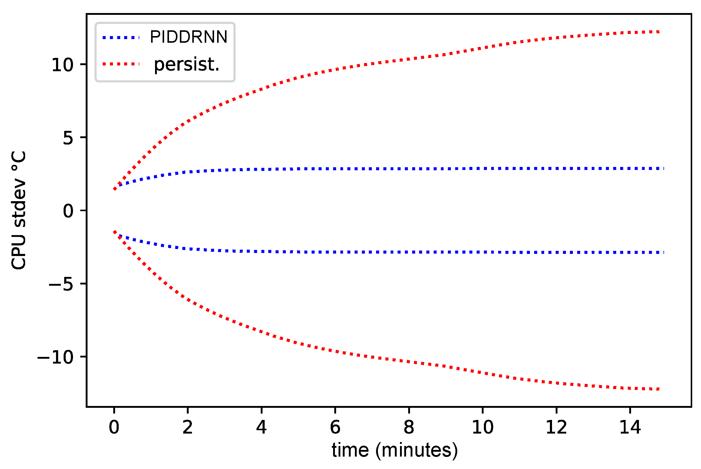
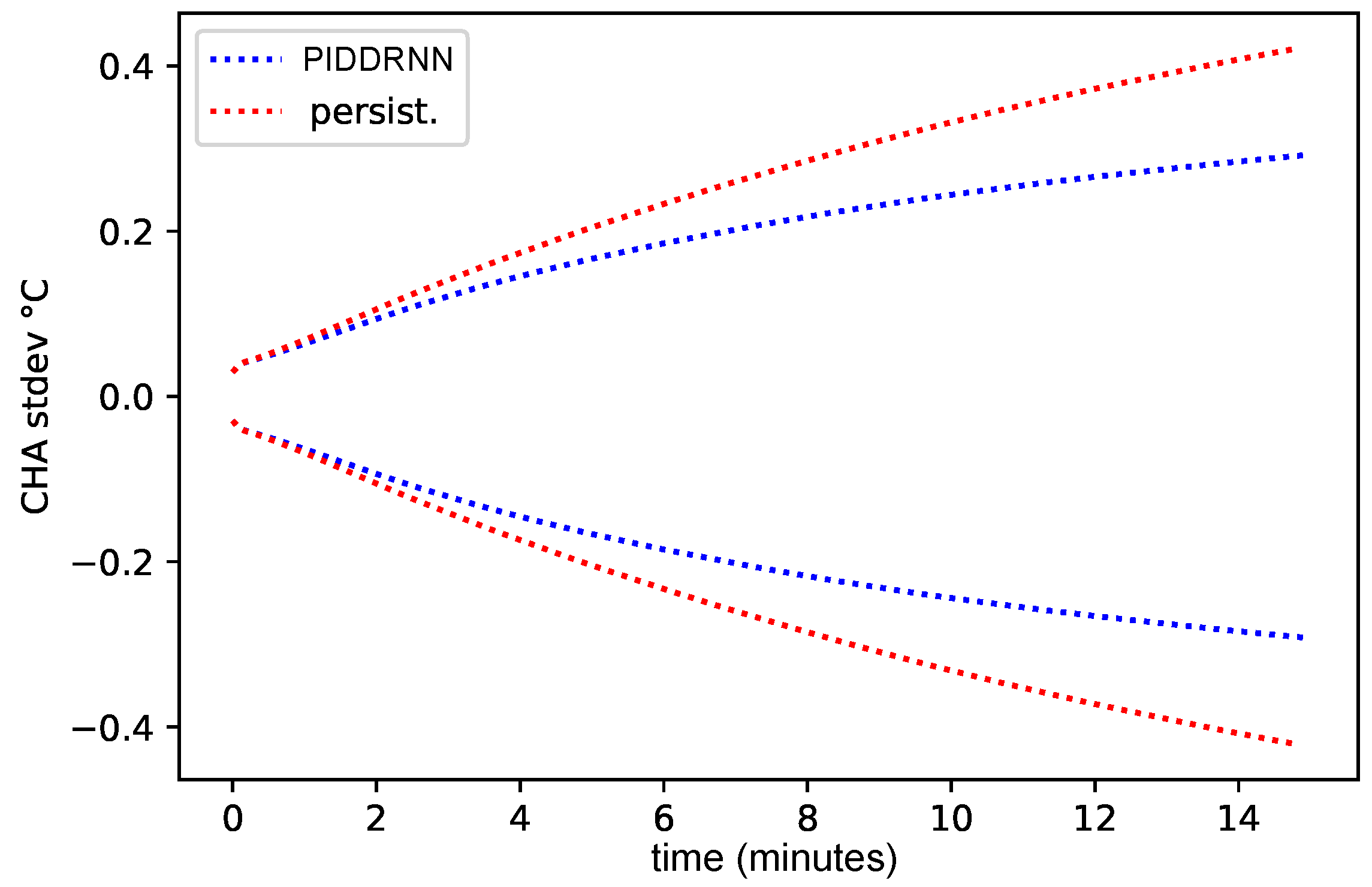
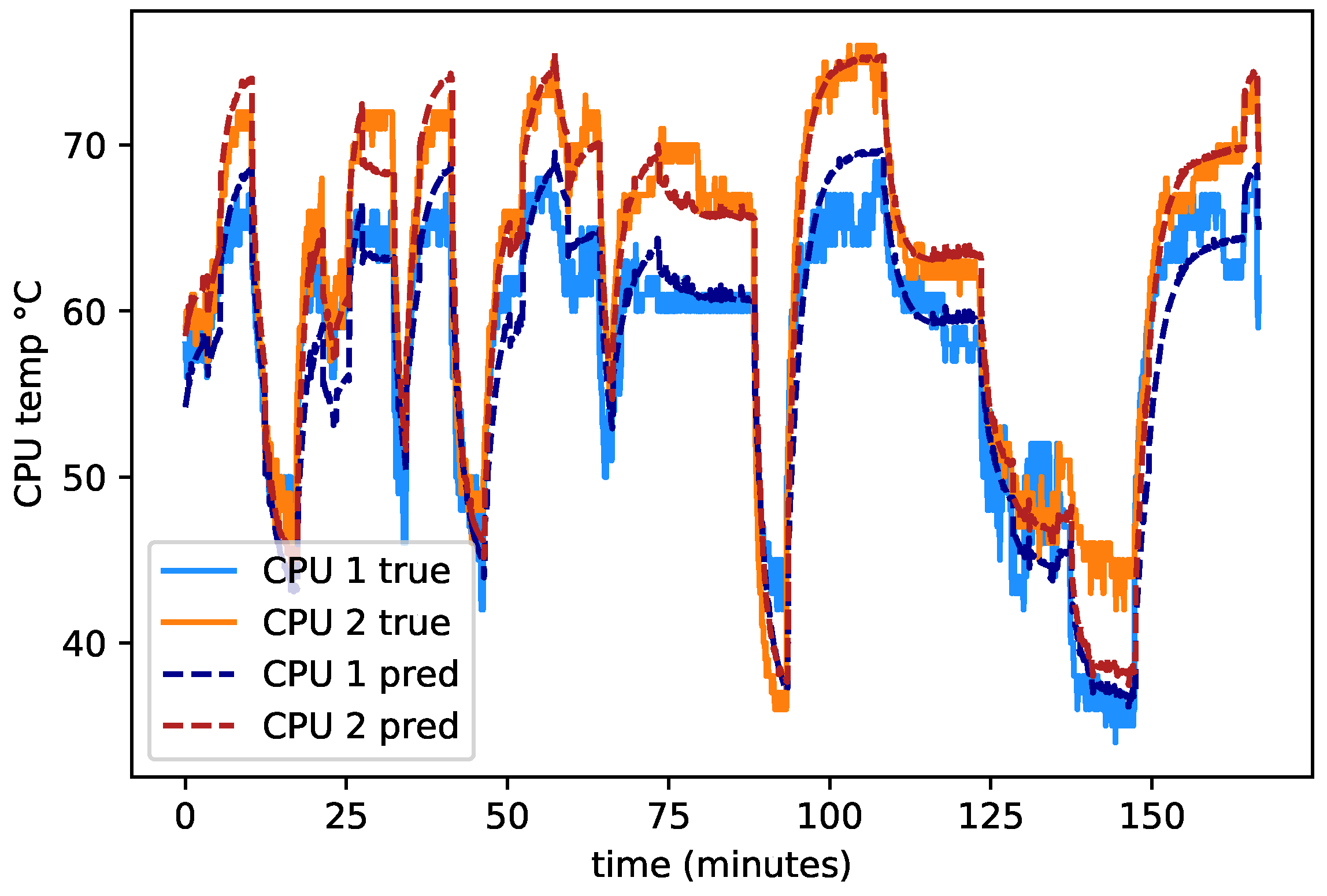
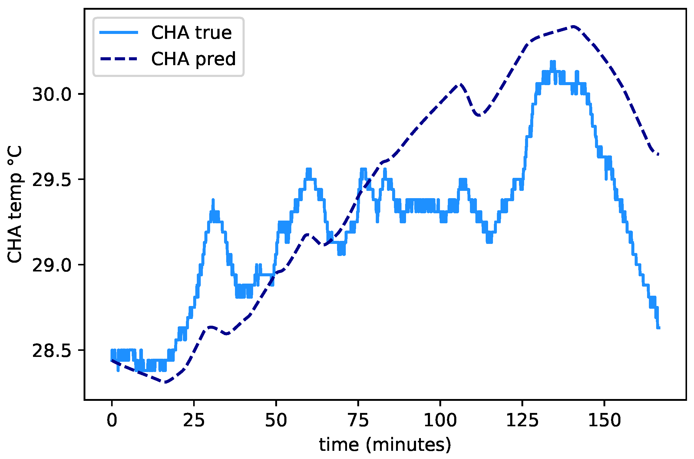
| PIDD RNN | 2.41 | 2.32 | 0.34 | 1.69 |
| Persistence | 6.93 | 7.54 | 0.38 | 4.95 |
| Standard RNN | 3.6 | 4.11 | 1.72 | 3.18 |
| Standard SSM | 3.04 | 2.98 | 1.97 | 2.66 |
| Mode | Epoch | CPU1 | CPU2 | Chamber |
|---|---|---|---|---|
| transfer | 0 | 2 | 2.02 | 0.85 |
| finetune | 1 | 1.84 | 1.67 | 0.72 |
| finetune | 10 | 1.88 | 1.53 | 0.74 |
| finetune | 100 | 1.9 | 1.47 | 0.66 |
| re-start | 100 | 2.2 | 1.96 | 1.63 |
Disclaimer/Publisher’s Note: The statements, opinions and data contained in all publications are solely those of the individual author(s) and contributor(s) and not of MDPI and/or the editor(s). MDPI and/or the editor(s) disclaim responsibility for any injury to people or property resulting from any ideas, methods, instructions or products referred to in the content. |
© 2023 by the authors. Licensee MDPI, Basel, Switzerland. This article is an open access article distributed under the terms and conditions of the Creative Commons Attribution (CC BY) license (https://creativecommons.org/licenses/by/4.0/).
Share and Cite
Brännvall, R.; Gustafsson, J.; Sandin, F. Modular and Transferable Machine Learning for Heat Management and Reuse in Edge Data Centers. Energies 2023, 16, 2255. https://doi.org/10.3390/en16052255
Brännvall R, Gustafsson J, Sandin F. Modular and Transferable Machine Learning for Heat Management and Reuse in Edge Data Centers. Energies. 2023; 16(5):2255. https://doi.org/10.3390/en16052255
Chicago/Turabian StyleBrännvall, Rickard, Jonas Gustafsson, and Fredrik Sandin. 2023. "Modular and Transferable Machine Learning for Heat Management and Reuse in Edge Data Centers" Energies 16, no. 5: 2255. https://doi.org/10.3390/en16052255