Article

Statistical Image Analysis on Liquid-Liquid Mixing Uniformity of Micro-Scale Pipeline with Chaotic Structure

1
State Key Laboratory of Complex Nonferrous Metal Resources Clean Utilization, Kunming University of Science and Technology, Kunming 650093, China
2
Faculty of Metallurgical and Energy Engineering, Kunming University of Science and Technology, Kunming 650093, China
*
Authors to whom correspondence should be addressed.
Energies 2023, 16(4), 2045; https://doi.org/10.3390/en16042045
Submission received: 7 November 2022 / Revised: 25 January 2023 / Accepted: 16 February 2023 / Published: 19 February 2023
(This article belongs to the Special Issue Advanced Analysis of Heat Transfer and Energy Conversion)

Abstract

:
The aim of this work is to introduce a novel statistical technique for quantifying the concentration field uniformity of the liquid-liquid mixing process within a micro-scale chaotic pipeline. For illustration, the microscale liquid-liquid mixer in which the inlet direction is parallel to the mixing unit is designed by using the chaotic pipeline with Baker map. Meanwhile, the non-uniformity coefficient method is adopted quantificationally instead of qualitatively estimating the concentration field uniformity of the chaotic micromixer based on uniform design theory and image analysis. Results show that the concentration distribution of the chaotic mixing process of liquid-liquid under various working conditions is obtained by solving the steady-state Navier–Stokes and diffusion convection equations. The average contribution ratio of the three basic mixing units of the chaotic Baker pipeline to the concentration field uniformity is approximately 6:3:1, which is calculated aligned with the fluid flow direction successively. The optimal mixing uniformity can be obtained as the initial velocity is 0.05 m/s and the diffusion coefficient is 5 × 10⁻⁹ m2/s, respectively. The reliability of the new method for estimating the concentration field uniformity parameters is explained from three dimensions. The statistical image analysis technique is illustrated to be reliable and effective in yielding accurate concentration field information of the simulated chaotic mixer. Furthermore, it can be adapted to examine a variety of concentration distribution issues in which concentrations are evaluated under distinct scales.

1. Introduction

Mixing processes aimed at achieving a homogeneous distribution of multi-component mixtures have a decisive influence on the overall performance of the specific reaction process. For instance, liquid-liquid mixing is crucial for a variety of engineering applications in the metallurgical, energy, mining, materials and chemical industries, as the quality of the final industrial products would be influenced by the mixing properties of the liquid-liquid strongly [1]. In the modern mineral industry, typically, hydrometallurgical processes have been widely used to extract metals from ores. In general, a large volume of ore slurry in stirred tanks is treated for leaching, digestion, precipitation, and other chemical processing to obtain pure metals or concentrated ores in mineral processing plants. Mixing intensification has been used to achieve mineral process intensification for the process industry [2]. In addition, the mixing of chemical substances is a necessary condition for chemical reactions in chemical or biological engineering and therefore has special significance. Then, the aim of mixing intensification is to increase production yield by improving fluid dynamics in the stirred tanks. Depending on the various processes or rectors involved, therefore, a variety of mixing intensification methods can be undertaken and have been widely used in recent years in order to intensify the mixing performance of fluids. It is worth noting that for process intensification, micro-fluidic techniques are effective and powerful techniques [3]. In fact, mixing at the molecular scale (i.e., micromixing) strongly influences the selectivity, yield, and quality of the final products in many biological or chemical processes. A great deal of investigations on micromixing processes from stirred tanks to static mixers of fluids has been done at different scales in order to better control biological or chemical processes [4]. The importance, urgency, and necessity of microscale devices in biological or chemical engineering have also increased significantly over the past two decades.
The fast development of microreactors has attracted the attention of many countries all over the world [5]. Micromixers can provide a much larger interfacial area that increases the rate of transport processes and, in turn, results in lower residence time [6]. Diffusive transport in micro-devices is faster than in conventional mixers in relation to the time scale of chemical kinetics. It has already been proved that reacting performance can be enhanced by using micro reaction technology significantly due to the nice mass and heat transport performances of the microreactors [7,8]. Therefore, two-phase flow in microsystems finds a great wide application in the chemical and biochemical industries, e.g., for extraction, aromatic nitration, emulsification, and separation [9]. Mixing fluids in passive micromixers is a very challenging task because advection is usually the dominant force in the pipelines of the micromixer. Strictly laminar fluid flow that is usually Reynolds number less than 100 and very low molecular diffusion coefficients (e.g., typically in the range from 10−9 m2/s to × 10−11 m2/s) fundamentally create tough mixing conditions [10]. These difficulties are usually achieved through special micromixer designs to generate chaotic fluid motion, usually at Reynolds numbers from 10 to 20. As a result, the contact surface between the fluids increases, which in turn accelerates diffusion mixing. Typical design and fluid mixing examples may be seen in Refs. [11,12,13]. It is generally accepted that it is necessary to develop multiple types of microreactors since micromixing performance is a critical feature in the development of microreactors.
Chaos theory has provided powerful and advanced theoretical guidance in the field of mixing process intensification. In fact, chaos has been widely used in various fields, such as time series (i.e., measurement signals) [14,15], combustion diagnosis [16], and flow field analysis [17,18,19], with special advantages in these fields [20]. For instance, a new concept named chaotic advection was introduced by Aref in 1984 in his paper published in the Journal of Fluid Mechanics. From the previous literature, the passive fluid particles are advected by a periodic laminar velocity field and exhibit chaotic trajectories. In fact, chaotic advection as a novel approach has been proposed to enhance the stretching and folding of species interfaces. It is a consensus that this deformation of the fluid-fluid boundaries increases the interfacial areas across which diffusion occurs and enhances the mixing efficiency [21]. For instance, Lee et al. (2011) summarized all kinds of chaotic mixers for micro-pipelines [22]. Liang et al. (2014) studied the mixing characteristics of the contraction-expansion helical mixer in the laminar regime, and it has been found to be superior in comparison to the regular helical mixer at a higher Reynolds number [23]. Adam et al. (2016) designed and fabricated a micromixer with short turning angles for self-generated turbulent structures. The mixing efficiency of 98% was obtained at a Reynolds number less than two [24].
The other issue is how to measure and evaluate the mixing state quality accurately and quantitatively under the guidance of chaotic mixing has always been an urgent issue to be solved. Besides, there is an increased desire to compare mixing performance for various working conditions. One of the biggest drawbacks of the classical methods for estimating concentration field distribution is the subjectivity of the measurement interpretation in most investigations on fluid mixing. Indeed, the distribution of the concentration field is typically determined with the sensory experience or the naked eye of several researchers. Different judgments may be produced or obtained when the same concentration field appears in front of different individuals or observed by the same operator many times. It is considered to have a quantitative measure of distribution uniformity by computers without human intervention. Fortunately, image processing technology has been used as a simple, practical, and effective approach to estimating concentration distribution. For instance, Yang et al. (2018) proposed a systematic image processing method for hydrodynamic characteristics of rectangular spouting beds with 30.2 mm and 101.6 mm and verified the feasibility and effectiveness of the image processing method in evaluating solid behavior in spouting beds [25]. Rivera et al. (2019) used image processing technology which is based on mathematical morphology, to measure flow pipelines and analyze the flow pipeline distribution of a parallel plate flow [26]. Li et al. (2019) proposed an approximate image processing method to study bubble characteristics in an active gas-solid fluidized bed, by which bubbles can be located, measured, and tracked from the results obtained by computational fluid dynamics and discrete element method [27]. Bai et al. (2021) used image processing technology to obtain a preliminary understanding and knowledge of bubble behavior during the carbon nanotube preparation process [28]. Soleimanian et al. (2021) used image processing technology and numerical simulation to determine the concentration of pollutants and verified the results of finite element simulation by experimental results [29]. Yang et al. (2022) used statistical image analysis to the processing of the two-phase flow mixing process in the top-blown gas-stirred tank [30]. Han et al. (2022) identified bubbles in a two-dimensional gas-solid fluidized bed with an image processing method to characterize bubble dynamics in a binary fluidization system and proposed a new empirical relation to estimating the change of bubble diameter along with the bed height [31]. Thus, it can be found that several studies of fluid mechanics have been carried out using image processing technology. In addition, there are also several existing statistical image analysis tools, including discrepancy measures, point-to-point measures, and volumetric measures to define the sample points’ equidistribution. To the best of our knowledge, however, no effective and powerful tool based on local discrepancy function and image analysis has been found to measure accurately and evaluate the state quality of the mixing process with chaotic structure quantitatively.
On the other hand, one of the classical methods for studying fluid mixing is numerical simulation. The basic idea is to mesh the geometry structure and internal fluid of the micromixer, calculate discreetly and iteratively, replace the results of the real flow field with the data of the grid, and finally get the flow field, concentration field, pressure field, and other contents needed by the micromixer [32]. A great deal of work has focused on fluid mixing with numerical simulation. For instance, Sui et al. (2012) investigated the increase in Reynolds number from steady-state laminar to transitional flows by numerical simulation [33]. Zhang et al. (2013) used the Giesekus constitutive model to conduct a direct numerical simulation of elastic turbulence of viscoelastic fluid at low Reynolds number in three-dimensional straight pipeline flow, obtained detailed information, investigated the statistical and structural characteristics of elastic turbulence, and verified the effect of elastic turbulence on enhancing fluid mixing [34]. By direct numerical simulation, Cai et al. (2018) discussed the flow patterns and the role of polymers playing in viscoelastic fluid flow to respectively figure out the underlying mechanism of efficient mixing and the occurrence of unstable flow motions [35]. Jost et al. (2020) quantified the mixing performance of a supercritical fluid-assisted crystallization reactor by using direct numerical simulation [36]. Thus, image processing and numerical simulation are promising methods for obtaining and analyzing the mixing uniformity and bubble behavior of single-phase, two-phase, and multiphase flows. Inspired and motivated by Xiao et al. (2017) [37], Ju et al. (2022) [38] and Yang et al. (2023) [39], in the present work, statistical image analysis technique based on statistical theory and image analysis is introduced to measure liquid-liquid mixing uniformity of micro-scale pipeline with chaotic structure.
The remainder of this article is organized as follows. In the next section (Section 2), the computational details of this work are listed. The methods used in this work are also described in detail in this section. The results of the simulations are presented and discussed in the third section (Section 3). The conclusions of this work are given in the fourth section (Section 4).

2. Experiments and Methods

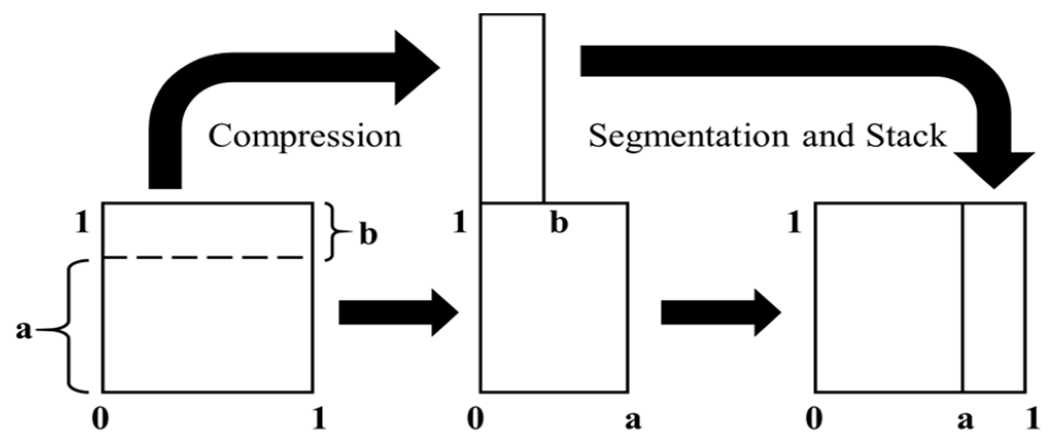
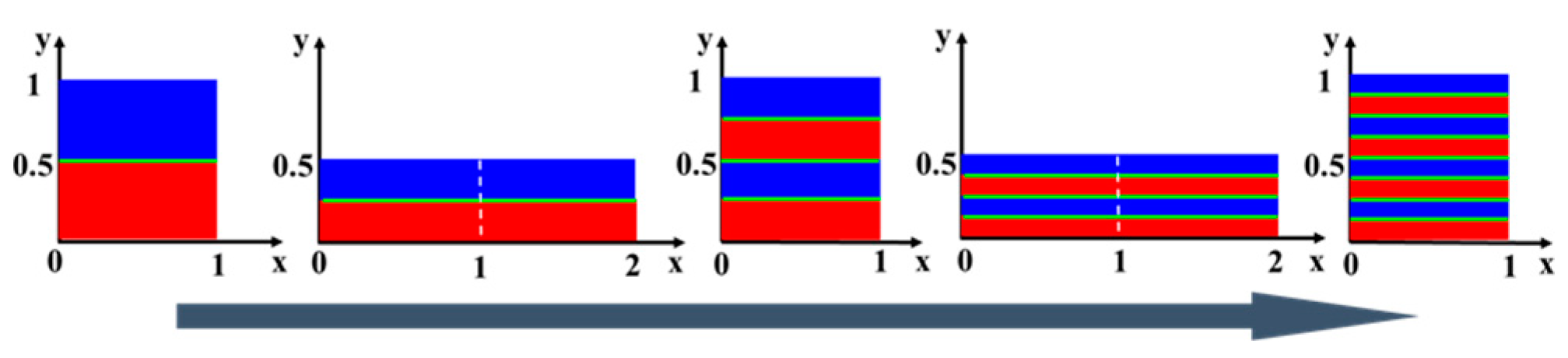
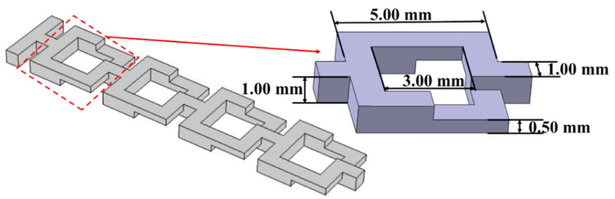
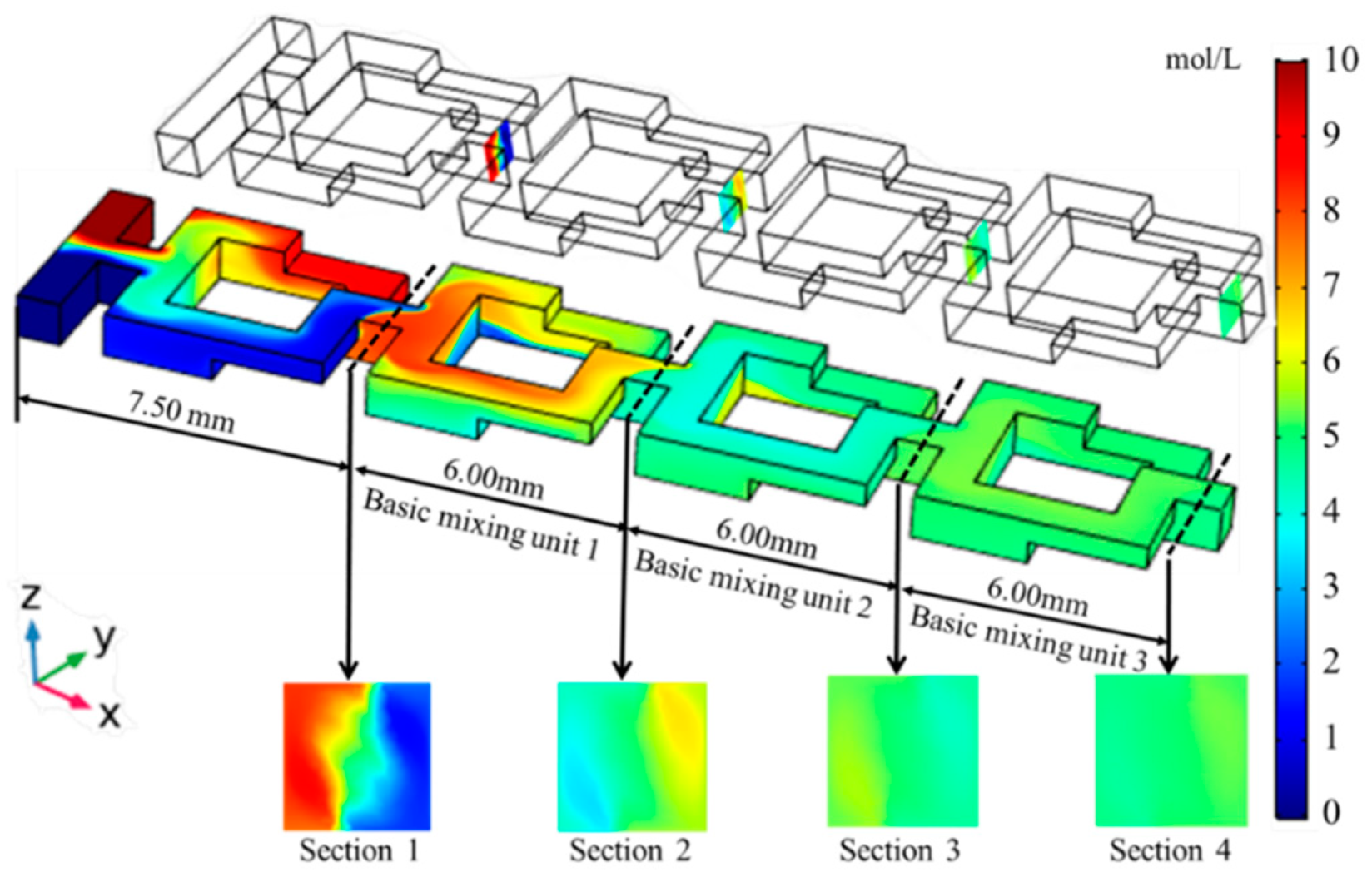
2.1. Fundamentals of Micromixer

Investigations on the flow behavior and mixing process in a wide variety of microchannels play a crucial role in the new or popular design for the passive micromixer of liquid-liquid. From open literature, Wang et al. (2007) have reported that the mixing efficiency in the diffusion channel of the passive micromixer of liquid-liquid with barriers is much greater than that without the barriers [38]. In this paper, a chaotic flow pipeline is constructed using the Baker constant-area chaotic map principle since the fluids mainly rely on molecular diffusion to mix in the laminar flow state, and the mixed fluids are generally incompressible, as shown in Figure 1. By selecting a = b = 0.5 in this figure, the chaotic Baker map shown in Figure 2 can be obtained. Blue and red represent different fluid cross-sections, while green represents the contact line between the two fluids, which reaches more layers as the fluid is compressed, stretched, cut, and stacked (the length of the green line increases gradually). The increase in the length of contact lines between different fluids means that it is easier and easier to mix depending on molecular diffusion. Based on the chaotic mixing theory, Baker-mixer was constructed according to Baker’s transformation to deeply understand the mechanism of chaotic mixing (see Figure 2). Baker-mixer has two samplings, and detection intakes with inlet and outlet sizes of 1.00 mm × 1.00 mm, and pipeline sizes are the same as in Ref. [40] for comparison. A mixing unit is defined as a basic mixing unit that periodically splits and merges. The Baker mixer has a single shunt combined structure with a mixer length of 7.00 mm. It should be noted that the pipeline of the mixing unit of the Baker mixer is reduced to half (0.50 mm) of the original pipeline (1.00 mm) in some places, and it is composed of four basic units, as shown in Figure 3.
The chaotic pipeline is a stratified and split combination that segments, stretches, and merges the fluid by changing the geometrical structure of the flow pipeline. This can increase the indirect contact area of different fluids and promote the mixing process between different fluids. The fluid flowing through the split pipeline may be rotated or squeezed and then gathered and layered. The number of layers after being superimposed can be multiplied by growth or exponential growth and ultimately greatly increase the contact area between fluids. At the same time, the branch pipelines of the layered split-combination micro-pipeline generally have a curved structure. When the fluid passes through this curved pipe, chaotic convection will occur in the three-dimensional space.

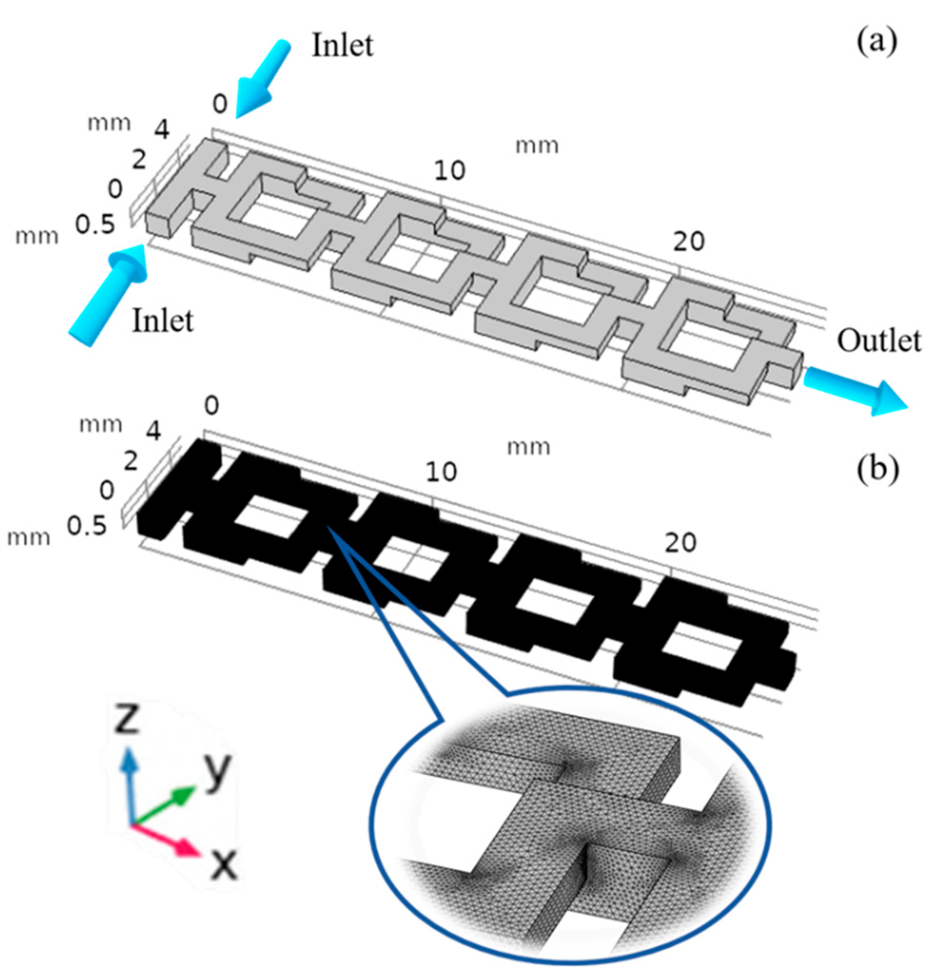
2.2. Numerical Simulations

All simulations discussed in this article are based on the finite element method using the calculation software. Here, the concentration transfer of liquid-liquid flow in a single micro-pipeline is simulated. The coupling of laminar flow and reactive flow transfer of dilute species is selected from the software for simulation. The control equations in this pre-set module include Navier–Stokes, continuity, and level set equations. In the model, the oil-water two-phase fluid in the micro-pipeline is an incompressible fluid, and the Navier–Stokes equation is given by
ρ u t · [ p I + η ( u + ( u ) T ) ] + ρ u · u = F
where ρ refers to the fluid density, u = ( u x ,   v y ,   w z ) refers to the velocity field, p refers to the fluid pressure, I refers to the unit diagonal matrix, η refers to the dynamic viscosity of the fluid, F = ( f x ,   f y ,   f z ) refers to the volume force that affects the fluid, and · u = 0 . Here, F = 0 because there are no volume forces. The following convection-diffusion equation describing the concentration of the dissolved substances in the fluid is given by
c t D 2 c = R u · c
where c refers to the concentration, D refers to the diffusion coefficient, and R refers to the reaction rate. In all the models, R = 0 because the concentration is not affected by any reactions. The Reynolds number, which represents the ratio between momentum and viscous friction, is given by
R e = ρ U L μ
where U is the flow rate, L is the characteristic length, and μ is the dynamic viscosity of the fluid. One of the significant things to note is that the characteristic size of an unmixed fluid block or lump is not simply calculated based on the diffusion coefficient and fluid residence time in the mixer. In other words, the flow of fluid is not only related to the change in the spatial position of fluid. In fact, the corresponding fluid structure changes while fluid flows in a chaotic micromixer, resulting in changes in fluid pressure and velocity. In addition, the contact surface between different fluids changes, and the degree of diffusion between fluids also changes. The final steady state of the fluid is dependent on the above Equations (1)–(3).
All simulations in this paper were performed using the dilute matter transfer module and the laminar flow module of computational software. The above combination coupled fluid flow with mass transfer, where the laminar flow Navier–Stokes equations are used to calculate the flow velocity field in the microtubes. For the simulation of the static mixers, the stability and reliability of the computational results in describing the laminar flow of incompressible fluids can also be verified by fractal evolution [41]. The velocity field is used in the convective diffusion equation to determine the turbidity map of the concentration distribution through the mixing operation. Both algorithms are based on Gaussian inversion methods. We set the normal velocity at the inlet and zero pressure value at the outlet with no slip along the wall. Generally, in laminar flow conditions, numerical simulations of mixing usually lead to high cell Peclet numbers. For high cell Peclet numbers, the numerical diffusion constant, i.e., the diffusion due to numerical errors, is comparable to or even larger than the actual diffusion to be studied in the simulation. In order to achieve sufficient numerical accuracy, numerical diffusion must be reduced by using adequate grid resolution and high-order difference schemes. In addition, we actually compared structured and unstructured meshes to structured and unstructured meshes. The main reason why an unstructured grid is used is that an unstructured grid has grid adaption, which can well characterize the laminar flow state of the boundary layer fluid. There is a better local encryption function, and there are many corner structures in the chaotic Baker channel, so numerical simulation with an unstructured grid can speed up the progress.
From Figure 4a, the angle between the two inlets of the chaotic Baker mixing channel is 180 degrees, and the outlet is perpendicular to the inlet direction. In Figure 4b, the mesh number of the mixer is composed of 1,618,302 cells, and these meshes have 370,633 mesh vertices. In terms of all the simulations in this work, the fluid considered for mixing is water at room temperature, and the scalar labeled particles based on the particle tracking method have no effect on the fluid flow in the chaotic Baker pipeline theoretically. In fact, the whole present model was initially filled with the fluid, whereas the fluid (water) entering through the pipeline inlet of the micromixer was marked with tracer particles to visualize the flow pattern of the fluid. All working condition parameters of numerical simulation are given in Table 1. In this work, each parameter of the initial velocity and diffusion coefficient were simulated, respectively, with a total of thirty-six working conditions. It should be emphasized that the hydrodynamic viscosity under all working conditions is 0.001 Pa·s. The outlet pressure was 0 Pa in all simulations, and the two inlet concentrations were defined as 1 mol/L and 10 mol/L, respectively. It is remarkable that the aim of this work is to quantify the concentration field of the passive chaotic mixer. Hence, the effect of solution rheology at the specific concentration was crucial for heat and mass transfer but not here. In addition, the boundary conditions of the steady state simulation set the velocity at the inlet to be uniform. In the case of constant input fluid parameters, the fluid flow state of the small-scale mixer changes after stabilization hardly. Meanwhile, a steady-state solver is here used for numerical simulation to reduce the occupation of computer resources and time cost. In order to better visualize the flow mixing mechanism inside a chaotic microstructure reactor with Baker pipeline, numerical simulations were envisaged to investigate the mixing effects caused by combining chaotic mixing and fluid stratification. The following assumptions were provided to build this required model: (1) changing in concentration did not change the viscosity and density of the fluid (i.e., dilute solution and no free convection); (2) it was assumed that the pipeline wall was smooth; and (3) the wall tension was ignored, and it was assumed that the medium was continuous.

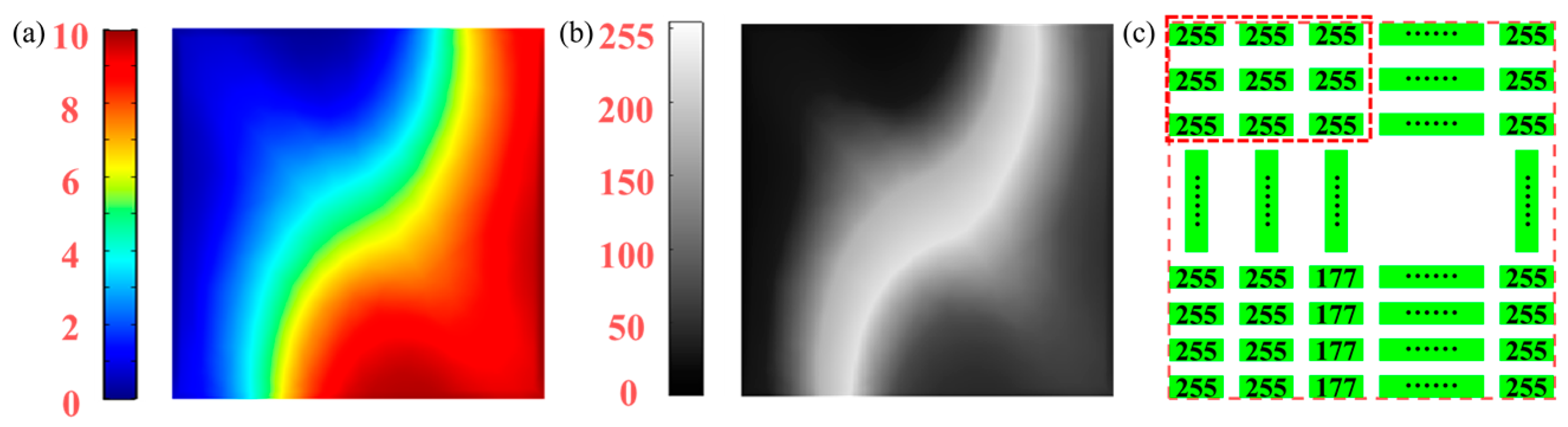
2.3. Proposed Method

According to the basic theory of applied mathematics, the flowing image obtained based on experiment or simulation can generally be considered a digital matrix. In fact, the value of each element in the digital matrix can correspond to the pixel value on the flowing image. In addition, the color-flowing image can be represented by three grayscale flowing images, and the grayscale flowing image is regarded as a matrix of which intensity is expressed as an integer value from the integer 0 to the positive integer 255. Let F u ( χ ) = x 1 x 2 x s be the uniform distribution function on the domain [ 0 ,   x ] = [ 0 , x 1 ] × [ 0 , x 2 ] × × [ 0 , x s ] where χ = { χ 1 , χ 2 , , χ N } for the N points and s = 2 in this paper. For [ 0 ,   x ] = [ 0 , x 1 ] × [ 0 , x 2 ] here, the empirical distribution function F x ( χ ) of the points set χ = { χ 1 , χ 2 , , χ N } is given by
F x ( χ ) = 1 N i = 1 N 1 [ 0 , x ] ( χ i )
where 1 [ 0 , x ] ( χ i ) is the indicator function and χ i = ( χ i 1 ,   χ i 2 ) [ 0 , x ] = [ 0 , x 1 ] × [ 0 , x 2 ] . Then, the L2-discrepancy is defined by
D 2 * ( x ) = [ C 2 | F x ( χ ) F u ( χ ) | 2 d χ ] 1 2
where D 2 * ( x ) can be defined as the L2-norm of the difference between theoretical distribution function F u ( χ ) and empirical distribution function F x ( χ ) . For the special rectangle region [ 0 , 1 ] = [ 0 ,   1 ] × [ 0 ,   1 ] , the quantity N of the encapsulated points can be counted. For [ 0 , x ] = [ 0 , x 1 ] × [ 0 , x 2 ] [ 0 , 1 ] = [ 0 ,   1 ] × [ 0 ,   1 ] , therefore, the local discrepancy function d x * ( χ ) for chaotic micromixer is given by
d x * ( χ ) = F x ( χ ) F u ( χ ) = 1 N c a r d ( χ [ 0 ,   x ] ) x 1 x 2
where c a r d ( χ [ 0 , x ] ) denotes the number of points in the intersection between χ and [ 0 , x ] . The following technique is based on image analysis. First, color (RGB) images that record the distribution of concentration fields can be converted to grayscale images by utilizing free mathematical software. The grayscale image is then converted into a digital matrix of which the numerical size of the elements represents the pixel value of the grayscale image) using the internal functions of the free mathematical software. In this work, using the mathematical analogy of the local discrepancy function, the concentration local discrepancy function (CLDF) of the local rectangular region θ = [ 0 ,   θ 1 ] × [ 0 , θ 2 ] in a real concentration field is given by
d P Q * ( θ ) = j = 1 θ 2 i = 1 θ 1 T i j j = 1 Q i = 1 P T i j θ 1 θ 2 P Q
where Tij denotes the concentration value at the position of the chaotic micromixer. Here, the CLDF is deemed superior over the local discrepancy function since CLDF is adopted to evaluate concentration field uniformity of the whole object surface by imaging video camera, whereas the local discrepancy function is restricted to a point set, namely concentration measurements at a specific point, by probe. This is the main merit of the proposed method for chaotic micromixers. Nevertheless, it is also immediately clear from above that d P Q * ( θ ) is dependent on the orientation of the first location for calculation. In order to address this shortcoming, four CLDFs from top-left, bottom-left, bottom-right and top-right orientations correspond to q = 1 , 2 , 3 , 4 , respectively, are calculated in this work.
In fact, the concept of separation intensity was first proposed by Danckwerts and has become a frequent means used by researchers to characterize mixing effects. The mathematical meaning is the ratio of the variance of the actual measured concentration of the mixed fluid to the variance of the completely separated system (i.e., unmixed). Thus, in the case of complete separation, the separation strength value is one. When mixed evenly, the separation strength is zero. Therefore, the smaller the separation strength value, the better the mixing effect of the fluid. Obviously, this criterion is consistent with that of the proposed statistical image analysis method of the chaotic mixer in this paper. However, this method has the measurement advantage with a plane or surface instead of a point, reducing information loss and increasing the accuracy of evaluation results. Figure 5 presents a brief illustration of the geometric sense of CLDF with the above four different start positions. Figure 5a shows the RGB concentration field, and Figure 5b shows the grayscale concentration field that both are demonstrated by two digital images with 100 × 100 = 104 values. Grayscale images are later converted from the former color file, which can consist of real concentration measurements or RGB concentration images. From Figure 5c, the two dashed lines (i.e., red and pink) represent the local and global rectangle regions, respectively. The CLDF is obtained easily using the gray intensity level matrix converted from a real concentration field. For q = 1 , 2 , 3 , 4 , the single non-uniformity coefficient NUCq of concentration field distribution of chaotic micromixer is given by
N U C q = sup θ 1 [ 1 , P ] , θ 2 [ 1 , Q ] | d P Q * ( θ , q ) |
where | d P Q * ( θ , q ) | denotes the absolute value of d P Q * ( θ , q ) . In detail, NUC1, NUC2, NUC3 and NUC4 denote the inhomogeneous degree of concentration distribution for chaotic micromixer in the whole rectangle surface of the object, corresponding to top-left, bottom-left, bottom-right and top-right orientations, respectively. The new index, non-uniformity coefficient (NUC), employed for uniformity evaluation of concentration field distribution of chaotic micromixer is given by
N U C = max { N U C 1 , N U C 2 , N U C 3 , N U C 4 }
where max { · } denotes the largest value in the set { · } . In general, if the concentration field is reasonably equidistributed for chaotic micromixers, it is expected that the proportion of the sum of concentration measurements within the smaller region is proportionately smaller. Simply, a smaller NUC denotes a uniformly distributed concentration field of chaotic micromixer while a large NUC indicates a poorly distributed temperature field of chaotic micromixer.

3. Results and Discussion

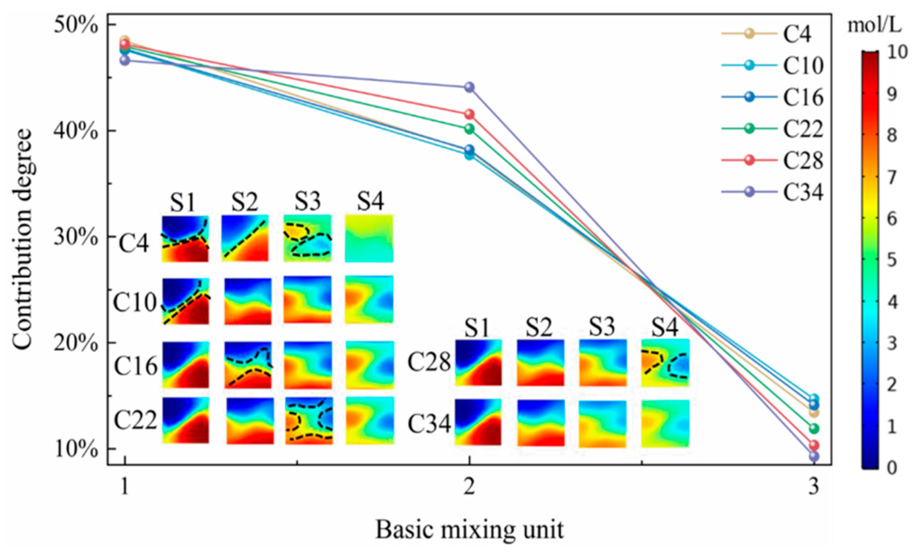
3.1. Mixing Performance of Basic Mixing Unit

Since NUC represents a non-uniformity coefficient, a larger NUC value indicates a greater degree of non-uniformity, and a smaller NUC value means more uniformity. By observing the concentration distribution nephogram of each section and the size relationship of the corresponding NUC value, and considering that there is no obvious different fluid boundary in the concentration distribution nephogram of each section, it is considered that the fluid has been mixed well, and the NUC value is not greater than 0.0075 is determined as complete mixing. With the help of the above numerical simulation of the thirty-six working conditions, the quantitative results of the mixing effect of the chaotic Baker pipeline under various working conditions are obtained by the uniformity analysis of the concentration distribution nephogram section under these working conditions by NUC method, as shown in Table 2. According to this table, in addition, as the diffusion coefficient increases, the characteristic length, which is directly proportional to the diffusion coefficient, increases gradually, but the corresponding NUC values do not change in the same trend. It is indicated that the numerical diffusion is eliminated while performing the calculation of the non-uniformity coefficient.
It is divided into five sections in this paper in order to explore the contribution of each basic mixing unit to the mixing process of the chaotic Baker mixing pipeline. The cut-off position is shown in Figure 6. Between every two adjacent sections is the basic mixing unit of chaotic Baker pipeline, and its structure is shown above. The six broken lines in each area in Figure 7 have the same diffusion coefficient, which are 10−13 m2/s (a), 10−11 m2/s (b), 10−10 m2/s (c), 5 × 10⁻¹⁰ m2/s (d), 10−9 m2/s (e), and 5 × 10⁻⁹ m2/s (f), respectively. From top to bottom in the legend of the same area, the initial velocity is 0.0001 m/s for C1, C7, C13, C19, C25 and C31, 0.0005 m/s for C2, C8, C14, C20, C26 and C32, 0.001 m/s for C3, C9, C15, C21, C27 and C33, 0.005 m/s for C4, C10, C16, C22, C28 and C34, 0.01 m/s for C5, C11, C17, C23, C29 and C35, and 0.05 m/s for C6, C12, C18, C24, C30 and C36. By observing the broken line diagram under various working conditions in this figure, it is easy to conclude that with the increase of mixing path, the NUC value decreases and the uniformity of fluid mixing increases. With the increase of the mixing path, the decrease of NUC value becomes smaller and smaller.
In order to explore the contribution of the basic mixing unit to the mixing process, the NUC values of each section under all working conditions are extracted and calculated in this paper. In fact, the concentration degree or concentration ratio is given by
C i , j = N U C i , k N U C i , k 1 N U C i , 4 N U C i , 1
where i = 1 ,   2 , ,   36 indicates the number of working conditions, j = 1 ,   2 ,   3 indicates the ordinal number of the hybrid unit, k = 2 ,   3 ,   4 indicates the number of sections, Ci,j indicates the contribution of the jth mixing unit in the ith case, and NUCi,k denotes the NUC value of the kth section of the ith working condition. By the statistical calculation of the NUC values of all sections of the thirty-six working conditions, it can be concluded that the proportion of the contribution of the basic mixing unit is roughly 6:3:1 (basic mixing units 1, 2, and 3). In Figure 8, the abscissa S1–S2 represents the basic mixing unit 1, S2–S3 represents the basic mixing unit 2, and S3–S4 represents the basic mixing unit 3. At the same time, when the initial velocity is the same (U0 = 0.005 m/s), the NUC value of the broken purple line (working conditions C4, C10, C16, C22, C28 and C34) decreases the fastest with the increase of the unit mixing path. By calculation, it can be obtained that for every 1.00 mm increase of the mixing path, the NUC decreases by 0.004035, 0.004376, 0.004099, 0.004082, 0.004053 and 0.004098 corresponding to working conditions C4, C10, C16, C22, C28 and C34, respectively. Under the corresponding working conditions, the average mixing efficiency of the mixing unit for basic mixing units 1, 2 and 3 is 47.740%, 39.962% and 12.295%, respectively.
It can also be observed from Figure 8 that in the above working conditions, the contribution ratio of each mixing unit is highly coincident, and the shape of the corresponding concentration distribution nephogram is roughly the same, which shows that the quantitative uniformity description of NUC value is consistent with the actual situation of the concentration distribution nephogram of numerical simulation. Combined with Figure 7 and Figure 8, although working conditions C4, C10, C16, C22, C28 and C34 have faster mixing behavior (rapid reduction of NUC value), the final actual mixing effect is not better than other working conditions. From the sectional concentration nephogram diagram of most of the above working conditions in Figure 8, there is an obvious boundary between the two fluids. The black dotted line in the figure has roughly depicted the shape and size of the boundary between the two fluids. The concentration distribution nephogram corresponding to the same position under these working conditions is generally similar, which proves that the observation results of concentration nephogram under C4, C10, C16, C22, C28 and C34 working conditions are in good agreement with the corresponding NUC value, which can describe the contribution trend of basic mixing unit to the whole mixing process. This shows that the NUC value obtained by image processing has good reliability and better quantitative description ability.

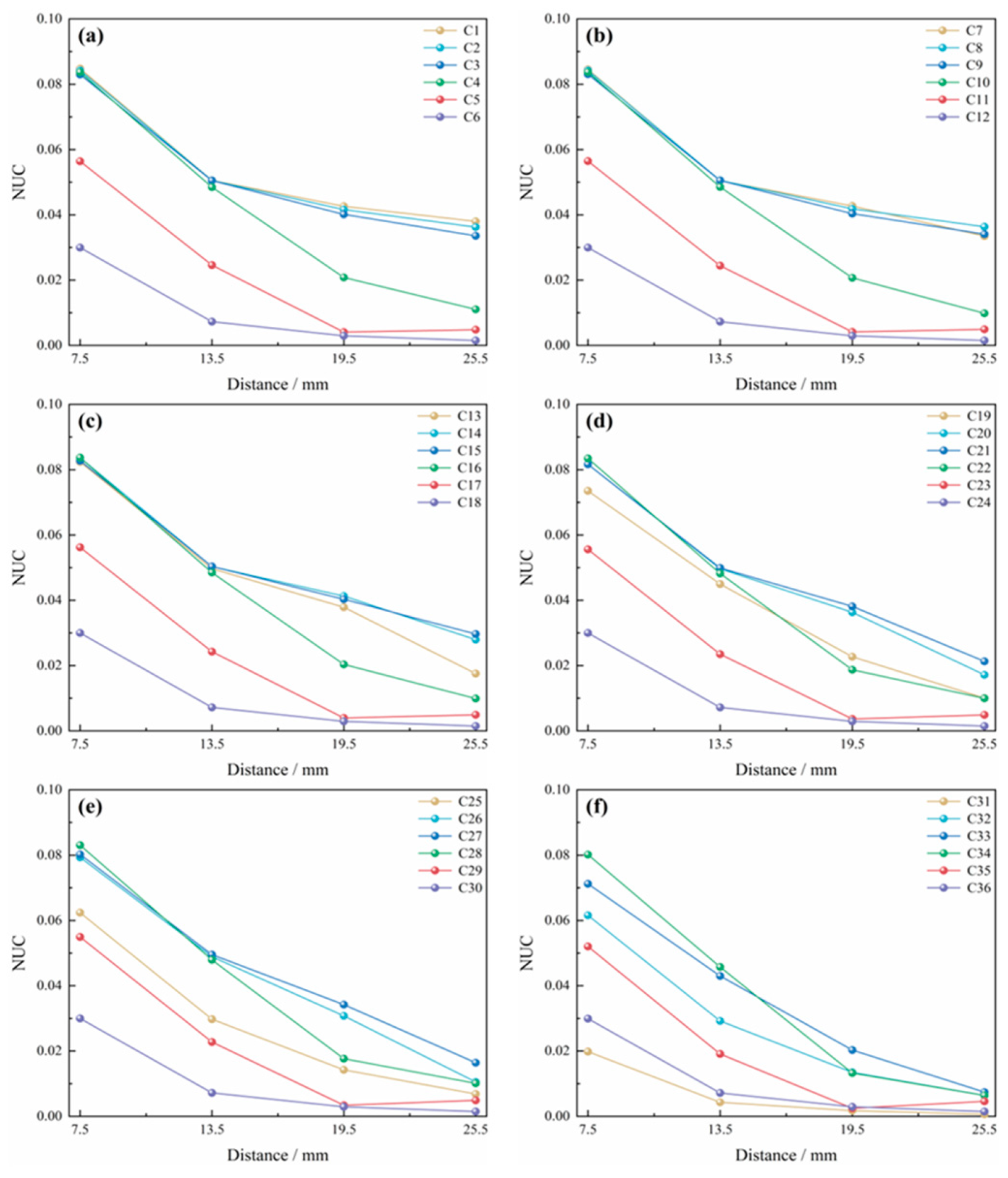
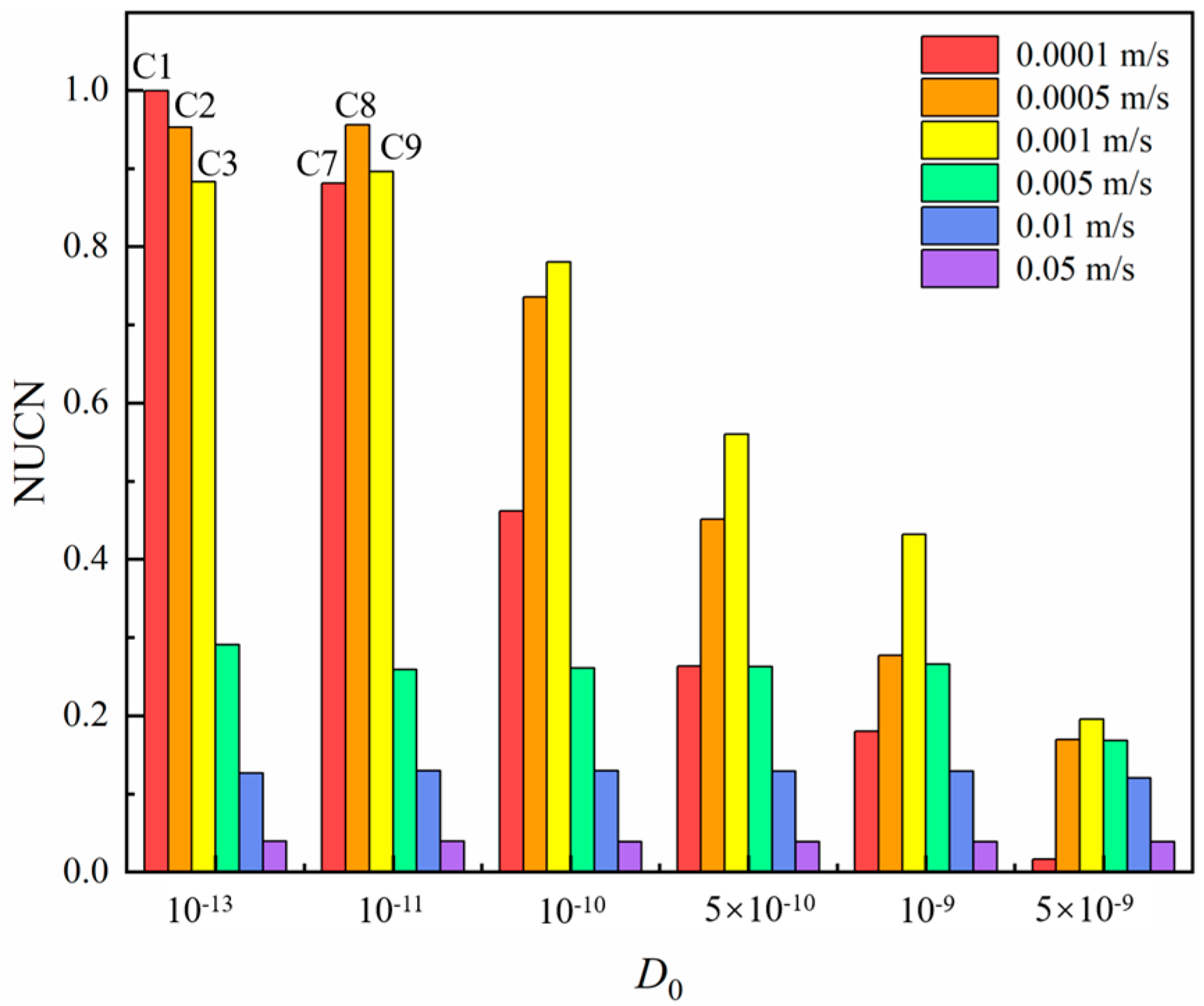
3.2. Effect of Diffusion Coefficient on Uniformity Coefficient

In order to facilitate the display of data, this paper normalizes the NUC data in Table 2. For instance, let the sampling interface of the first mixing unit be S0, and then the NUC values corresponding to working conditions C4, C10, C16, C22, C28 and C34 are 0.044456, 0.044457, 0.044465, 0.044497, 0.044532 and 0.044749, respectively, and the variance of the above six numbers is 1.06647 × 10⁻⁸. It is too small, indicating that there is no significant difference between the above values. It is, therefore, acceptable to normalize and compare S1 (in Figure 8) to the dashed line under this condition. The processing method is to divide all NUC values by 0.038 to get Table 3, and the data in Table 3 is called NUCN (i.e., non-uniformity coefficient normalization). It can be observed from Figure 9 that at the same inlet speed, the greater the diffusion coefficient, the smaller the corresponding NUCN value, which means the better the mixing effect. This is because when the diffusion coefficient is large, driven by the concentration gradient, the diffusion between different substance molecules is very intense, the mass of substance transported to another substance will be large, and finally show a very good mixing situation, and the corresponding NUCN value is also very small.
When the diffusion coefficient is small to a certain extent, the mixing degree will remain unchanged within a certain initial velocity range. It can also be seen from the red dotted box in Figure 10b for working conditions C1, C2, C3, C7, C8 and C9 that there is no obvious difference in the corresponding concentration distribution nephogram. Similarly, the maximum height difference of the histogram under the corresponding working conditions C1, C2, C3, C7, C8 and C9 in Figure 9 shall not exceed 11.83%. It can also be seen from the histogram in Figure 9 that the larger the diffusion coefficient, the better the mixing situation. With the decrease of the diffusion coefficient, the mixing degree gap between different diffusion coefficients is gradually narrowing, and the gap is narrowing from the initial 0.960031 to 0.17888, which is 81.37%. This is because when the diffusion coefficient is small, even under the same concentration nephogram, the mass of one substance diffusing to another substance will be very small, resulting in the decline of the mixing effect. The same conclusion can be drawn from the physical meaning of diffusion coefficient, which further confirms the correctness of NUC analysis of the uniformity of typical concentration distribution nephogram.

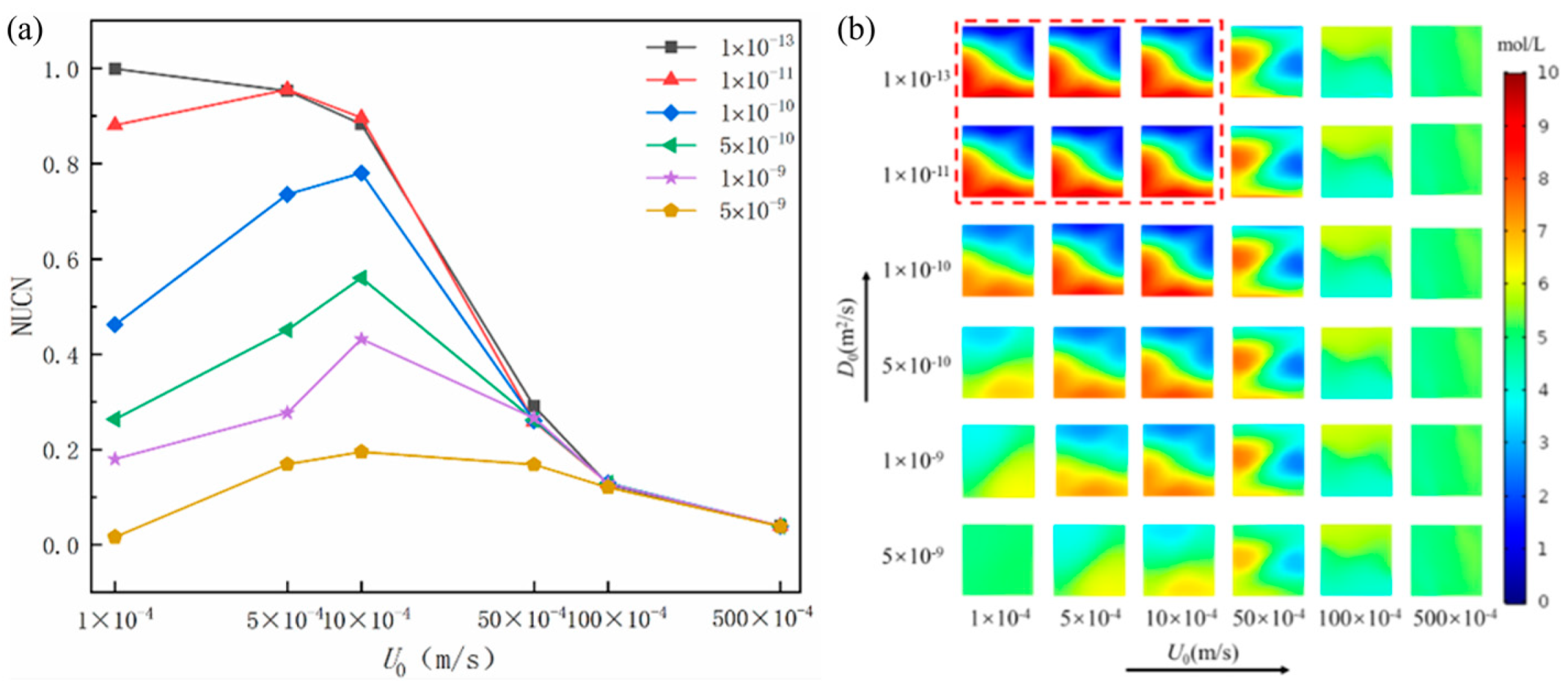
3.3. Effect of Initial Velocity on Uniformity Coefficient

It is worth mentioning that the diffusion coefficient is not correlated with the initial velocity. In fact, the diffusion coefficient of a molecule has been used to measure the diffusion ability between molecules of different substances and is one of the physical properties of a substance. It is well known from Fick’s law that the physical meaning of the diffusion coefficient is the amount of the mass of the substance diffused through the unit area per unit of time: the larger the diffusion coefficient, the more mass of the substance diffused through the unit area per unit time, and vice versa, the less. In this paper, Fick’s first law is observed in the simulation, and the diffusion coefficient is a constant that is related to the temperature, the viscosity of the fluid and the size of the molecules. Therefore, the diffusion coefficient and the initial velocity can exist as two independent variables to a certain extent. In order to compare the effect of initial velocity on the mixing efficiency of the chaotic Baker pipeline, numerical simulation was carried out for working conditions from C1 to C34 at different initial velocities, as shown in Table 1. As can be seen in Figure 10a, the broken line corresponds to the diffusion coefficient D0 = 5 × 10⁻⁹ m2/s, and the value of NUCN at a lower level throughout with the increase of initial velocity (<0.39800). It can be seen from Figure 10a that the mixing effect of the chaotic Baker pipeline increases with the increase of initial velocity according to the broken line corresponding to the diffusion coefficient D0 = 1 × 10⁻¹³ m2/s. The reason for this phenomenon is that when the diffusion coefficient is too small, convective mixing always dominates in the process of fluid mixing. With the increase of initial velocity, convective mixing intensifies, which further promotes the mixing effect of convective mixing on different liquids.
Under the condition of other diffusion coefficients, the mixing effect of the chaotic Baker pipeline first decreases and then increases. The reason for this trend is that when the diffusion coefficient is large, and the initial velocity is small, diffusion mixing plays a dominant role in the process of fluid mixing. However, with the increase of initial velocity, the proportion of convective mixing gradually increases and finally occupies a dominant position. This transition from diffusion mixing to convection mixing also leads to the corresponding change trend that the area of the green area first increases and then decreases in the concentration distribution nephogram of the outlet section under various working conditions in Figure 10b. By simply observing the nephogram of concentration distribution at the outlet section of D0 = 1 × 10⁻¹¹ m2/s in Figure 10b with the naked eye, in particular, it cannot be concluded that the mixing effect tends to decline first and then rise, which seems to be inconsistent with the broken line trend corresponding to D0 = 1 × 10⁻¹¹ m2/s in Figure 10a. On the contrary, this inconsistency shows that NUC has an amplification effect, which can amplify and accurately measure the differences that researchers cannot detect with the naked eye.
In response to the introduction of the new mixing uniformity metric, furthermore, it is more descriptive of the state in which mixing occurs during the mixing process but not completely mixed. The value obtained from the fully biased CLDF is closer to one compared to the other cases, while the value obtained from the fully blended CLDF is closer to zero up to 10−7. Clearly, the CLDF is better suited to describe the more homogeneous cases. This is due to the fact that CLDF describes the degree of difference between a pixel point and the surrounding pixel points. In addition, the image information is transformed from RGB values to grayscale values during the actual computational processing, and the data information is dimensionally reduced, which is beneficial to the speed of data processing but eventually leads to a certain amount of error. However, it still cannot be denied that this method is practical and stable. The question about the size of the local bias size does not affect CLDF, because we perform image processing starting from a single pixel point, which is already the smallest scale of the processable image information.

4. Conclusions

In this study, an evaluation model for the uniformity of concentration field in the mixing process of liquid-liquid flow in a chaotic micromixer is developed, and the concentration field in the fluid mixing process in a chaotic Baker pipeline is illustrated to evaluate the mixing performance of the new mixer. The contribution of this paper is to propose a parameter (i.e., non-uniformity coefficient) to effectively characterize the mixing performance of liquid-liquid flow in a chaotic micromixer and thereafter effectively quantify the complexity of the change of fluid concentration field in the mixing process of Baker micromixer. The effects of inlet velocity and fluid diffusion coefficient on fluid uniformity in the mixing process are investigated thoroughly, and the main conclusions are summarized as follows:
(1)
The contribution of the basic mixing unit of the chaotic Baker pipeline to the whole fluid mixing process is studied by using the non-uniformity coefficient (NUC) method under various conditions (thirty-six cases in this study). The experimental results show that the optimal contribution ratio of the basic mixing unit is about 6:3:1 (calculated in turn along the fluid flow direction), which can provide theoretical guidance for the structural design of the millimeter mixer.
(2)
The effects of two parameters (initial velocity and diffusion coefficient) on the quality of the mixing state in the mixing process of liquid-liquid flow are investigated thoroughly, and the uniformity of the fluid concentration field under different experimental conditions is calculated. It is found that the highest mixing uniformity can be achieved when the initial velocity U0 = 0.05 m/s, and the diffusion coefficient D0 = 5 × 10⁻⁹ m2/s.
(3)
Based on image processing technology, under thirty-six different working conditions, it is analyzed from three dimensions: the contribution of the basic mixing unit of the chaotic Baker pipeline, the diffusion coefficient, and the influence of initial velocity on fluid mixing in the chaotic Baker pipeline. The experimental results show that the non-uniformity coefficient method can evaluate the characteristics of the macro mixing process and provide a method for directly measuring the uniformity of the macro mixing process. The statistical image analysis technique based on uniform design theory is illustrated to be reliable and effective in yielding accurate concentration field information of the simulated chaotic mixer. Meanwhile, it is also found that the quantification of the non-uniformity coefficient method can also amplify the difference.

Author Contributions

Conceptualization, J.W. and Q.X.; methodology, Q.X.; software, H.W. (Haotian Wang); validation, H.W. (Hua Wang); formal analysis, K.Y.; investigation, K.Y.; resources, H.W. (Haotian Wang); data curation, K.Y.; writing—original draft preparation, H.W. (Haotian Wang); writing—review and editing, Q.X.; visualization, H.W. (Haotian Wang); supervision, Q.X.; project administration, Q.X.; funding acquisition, Q.X. All authors have read and agreed to the published version of the manuscript.

Funding

This research was funded by the Yunnan Fundamental Research Project, China (No. 202201BE070001-026), Natural Science Foundation of Yunnan Province, China (No. 202101AU070031), Interdisciplinary Research Project of Kunming University of Science and Technology (No. KUST-xk2022001), Young Talent Training Program for Science and Technology Think Tank by China Association for Science and Technology, China (No. 20220615ZZ07110003), and Young Elite Scientist Sponsorship Program by China Association for Science and Technology, China (No. YESS20210106).

Data Availability Statement

Not applicable.

Acknowledgments

The authors wish to especially thank the referees for the numerous detailed questions and comments that greatly improved the presentation.

Conflicts of Interest

The authors declare no conflict of interest.

References

  1. Valdés, J.P.; Kahouadji, L.; Matar, O.K. Current advances in liquid-liquid mixing in static mixers: A review. Chem. Eng. Res. Des. 2022, 177, 694–731. [Google Scholar] [CrossRef]
  2. Chen, X.; Li, T. A novel passive micromixer designed by applying an optimization algorithm to the zigzag microchannel. Chem. Eng. J. 2017, 313, 1406–1414. [Google Scholar] [CrossRef]
  3. Li, X.; Jiang, F.; Ravindra, A.V.; Zhou, J.; Zhou, A.; Le, T.; Peng, J.; Ju, S. Mixing processes in a 3D printed large-flow microstructured reactor: Finite element simulations and experimental study. Chem. Eng. J. 2019, 370, 295–304. [Google Scholar] [CrossRef]
  4. Le The, H.; Le Thanh, H.; Dong, T.; Ta, B.Q.; Tran-Minh, N.; Karlsen, F. An effective passive micromixer with shifted trapezoidal blades using wide Reynolds number range. Chem. Eng. Res. Des. 2015, 93, 1–11. [Google Scholar] [CrossRef]
  5. Ruijin, W.; Beiqi, L.; Dongdong, S.; Zefei, Z. Investigation on the splitting-merging passive micromixer based on Baker’s transformation. Sens. Actuators B 2017, 249, 395–404. [Google Scholar] [CrossRef]
  6. Glatzel, T.; Litterst, C.; Cupelli, C.; Lindemann, T.; Moosmann, C.; Niekrawietz, R.; Streule, W.; Zengerle, R.; Koltay, P. Computational fluid dynamics (CFD) software tools for microfluidic applications—A case study. Comput. Fluids 2008, 37, 218–235. [Google Scholar] [CrossRef]
  7. Kim, D.S.; Lee, S.W.; Kwon, T.H.; Lee, S.S. A barrier embedded chaotic micromixer. J. Micromech. Microeng. 2004, 14, 798–805. [Google Scholar] [CrossRef]
  8. Han, Q.; Liu, Z.; Li, W. Enhanced thermal performance by spatial chaotic mixing in a saw-like microchannel. Int. J. Therm. Sci. 2023, 186, 108148. [Google Scholar] [CrossRef]
  9. Verma, R.K.; Ghosh, S. Two-phase flow in miniature geometries: Comparison of gas-liquid and liquid-liquid flows. ChemBioEng Rev. 2019, 6, 5–16. [Google Scholar] [CrossRef] [Green Version]
  10. Luo, X.; Cheng, Y.; Zhang, W.; Li, K.; Wang, P.; Zhao, W. Mixing performance analysis of the novel passive micromixer designed by applying fuzzy grey relational analysis. Int. J. Heat Mass Transfer 2021, 178, 121638. [Google Scholar] [CrossRef]
  11. Okuducu, M.B.; Aral, M.M. Novel 3-D T-shaped passive micromixer design with helicoidal flows. Processes 2019, 7, 637. [Google Scholar] [CrossRef] [Green Version]
  12. Hossain, S.; Ansari, M.A.; Kim, K.Y. Evaluation of the mixing performance of three passive micromixers. Chem. Eng. J. 2009, 150, 492–501. [Google Scholar] [CrossRef]
  13. Mondal, B.; Mehta, K.S.; Patowari, K.P.; Pati, S. Numerical study of mixing in wavy micromixers: Comparison between raccoon and serpentine mixer. Chem. Eng. Process. 2019, 136, 44–61. [Google Scholar] [CrossRef]
  14. Zhang, J.; Dong, X.; Ma, H.; Li, X.; Feng, Y. Chaotic analysis of the concentration field in a submerged impinging stream mixer. Chem. Eng. Technol. 2015, 38, 1530–1536. [Google Scholar] [CrossRef]
  15. Yang, K.; Liu, J.; Wang, M.; Wang, H.; Xiao, Q. Identifying flow patterns in a narrow channel via feature extraction of conductivity measurements with a support vector machine. Sensors 2023, 23, 1907. [Google Scholar] [CrossRef]
  16. Ding, S.L.; Song, E.Z.; Yang, L.P.; Litak, G.; Wang, Y.Y.; Yao, C.; Ma, X.Z. Analysis of chaos in the combustion process of premixed natural gas engine. Appl. Therm. Eng. 2017, 121, 768–778. [Google Scholar] [CrossRef]
  17. Zhang, L.; Yang, K.; Li, M.; Xiao, Q.; Wang, H. Enhancement of solid-liquid mixing state quality in a stirred tank by cascade chaotic rotating speed of main shaft. Powder Technol. 2022, 397, 117020. [Google Scholar] [CrossRef]
  18. Zhang, L.; Yang, K.; Li, M.; Xiao, Q.; Wang, H. Experimental investigation on the uniformity optimization and chaos characterization of gas-liquid two-phase mixing process using statistical image analysis. Adv. Powder Technol. 2021, 32, 1627–1640. [Google Scholar] [CrossRef]
  19. Zhang, L.; Yang, K.; Li, M.; Xiao, Q.; Wang, H. Chaotic characterization of macromixing effect in a gas-liquid stirring system using modified 0-1 test. Can. J. Chem. Eng. 2022, 100, 261–275. [Google Scholar] [CrossRef]
  20. Yuan, S.; Zhou, M.; Peng, T.; Peng, T.; Li, Q.; Jiang, F. An investigation of chaotic mixing behavior in a planar microfluidic mixer. Phys. Fluids 2022, 34, 032007. [Google Scholar] [CrossRef]
  21. Zhang, K.; Guo, S.; Zhao, L.; Zhao, X.; Chan, H.L.; Wang, Y. Realization of planar mixing by chaotic velocity in microfluidics. Microelectron. Eng. 2011, 88, 959–963. [Google Scholar] [CrossRef]
  22. Lee, C.Y.; Chang, C.L.; Wang, Y.N.; Fu, L.M. Microfluidic mixing: A review. Int. J. Mol. Sci. 2011, 12, 3263–3287. [Google Scholar] [CrossRef] [PubMed] [Green Version]
  23. Liang, D.; Zhang, S. A contraction-expansion helical mixer in the laminar regime. Chin. J. Chem. Eng. 2014, 22, 261–266. [Google Scholar] [CrossRef]
  24. Adam, T.; Hashim, U. Design and fabrication of micro-mixer with short turns angles for self-generated turbulent structures. Microsyst. Technol. 2016, 22, 433–440. [Google Scholar] [CrossRef]
  25. Yang, J.; Breault, R.W.; Rowan, S.L. Applying image processing methods to study hydrodynamic characteristics in a rectangular spouted bed. Chem. Eng. Sci. 2018, 188, 238–251. [Google Scholar] [CrossRef]
  26. Rivera, F.F.; Hidalgo, P.E.; Castañeda-Záldivar, F.; Terol-Villalobos, I.R.; Orozco, G. Phenomenological behavior coupling hydrodynamics and electrode kinetics in a flow electrochemical reactor. Numerical analysis and experimental validation. Chem. Eng. J. 2019, 355, 457–469. [Google Scholar] [CrossRef]
  27. Li, J.; Agarwal, R.K.; Zhou, L.; Yang, B. Investigation of a bubbling fluidized bed methanation reactor by using CFD-DEM and approximate image processing method. Chem. Eng. Sci. 2019, 207, 1107–1120. [Google Scholar] [CrossRef]
  28. Bai, W.; Chu, D.; He, Y. Bubble characteristic of carbon nanotubes growth process in a tapered fluidized bed reactor without a distributor. Chem. Eng. J. 2021, 407, 126792. [Google Scholar] [CrossRef]
  29. Soleimanian, N.; Akhtarpour, A. A new method for estimating pollutant concentration in unsaturated soil using digital image processing technique. J. Phys. Conf. Ser. 2021, 1973, 012204. [Google Scholar] [CrossRef]
  30. Yang, K.; Zhang, X.; Li, M.; Xiao, Q.; Wang, H. Measurement of mixing time in a gas-liquid mixing system stirred by top-blown air using ECT and image analysis. Flow Meas. Instrum. 2022, 84, 102143. [Google Scholar] [CrossRef]
  31. Han, B.; Sun, Z.; Zhu, J.; Fu, Z.; Kong, X.; Barghi, S. Bubble dynamics in 2-D gas-solid fluidized bed with Geldart A or Geldart B particles by image processing method. Can. J. Chem. Eng. 2022, 100, 3588–3599. [Google Scholar] [CrossRef]
  32. Mouza, A.A.; Patsa, C.M.; Schönfeld, F. Mixing performance of a chaotic micro-mixer. Chem. Eng. Res. Des. 2008, 86, 1128–1134. [Google Scholar] [CrossRef]
  33. Sui, Y.; Teo, C.J.; Lee, P.S. Direct numerical simulation of fluid flow and heat transfer in periodic wavy channels with rectangular cross-sections. Int. J. Heat Mass Transfer 2012, 55, 73–88. [Google Scholar] [CrossRef]
  34. Zhang, H.N.; Li, F.C.; Cao, Y.; Tomoaki, K.; Yu, B. Direct numerical simulation of elastic turbulence and its mixing-enhancement effect in a straight channel flow. Chin. Phys. B 2013, 22, 024703. [Google Scholar] [CrossRef]
  35. Cai, W.H.; Li, Y.Y.; Zhang, H.N.; Li, Y.K.; Cheng, J.P.; Li, X.B.; Li, F.C. An efficient micro-mixer by elastic instabilities of viscoelastic fluids: Mixing performance and mechanistic analysis. Int. J. Heat Fluid Flow 2018, 74, 130–143. [Google Scholar] [CrossRef]
  36. Jost AM, D.; Glockner, S.; Erriguible, A. Direct numerical simulations of fluids mixing above mixture critical point. J. Supercrit. Fluids 2020, 165, 104939. [Google Scholar] [CrossRef]
  37. Xiao, Q.; Zhai, Y.; Lv, Z.; Xu, J.; Pan, J.; Wang, H. Non-uniformity quantification of temperature and concentration fields by statistical measure and image analysis. Appl. Therm. Eng. 2017, 124, 1134–1141. [Google Scholar] [CrossRef] [Green Version]
  38. Ju, Y.; Wu, L.; Li, M.; Xiao, Q.; Wang, H. A novel hybrid model for flow image segmentation and bubble pattern extraction. Measurement 2022, 192, 110861. [Google Scholar] [CrossRef]
  39. Yang, K.; Wang, Y.; Li, M.; Li, X.; Wang, H.; Xiao, Q. Modeling topological nature of gas–liquid mixing process inside rectangular channel using RBF-NN combined with CEEMDAN-VMD. Chem. Eng. Sci. 2023, 267, 118353. [Google Scholar] [CrossRef]
  40. Wang, R.; Lin, J.; Li, H. Chaotic mixing on a micromixer with barriers embedded. Chaos Solitons Fractals 2007, 33, 1362–1366. [Google Scholar] [CrossRef]
  41. Pishkoo, A.; Darus, M. Using fractal calculus to solve fractal Navier–Stokes equations, and simulation of laminar static mixing in COMSOL multiphysics. Fractal Fract. 2021, 5, 16. [Google Scholar] [CrossRef]
Figure 1. Illustration of the incompressible Baker map.
Energies 16 02045 g001
Figure 2. Schematic diagram of Baker transformation with fluid cross-sections in red and blue.
Energies 16 02045 g002
Figure 3. Geometric model of flow channel constructed by chaotic Baker map.
Energies 16 02045 g003
Figure 4. Considering geometry: (a) chaotic Baker pipeline model constructed in numerical simulation software; (b) enlarged view of structured mesh.
Energies 16 02045 g004
Figure 5. Brief illustration of CLDF with different start position selections: (a) RGB image; (b) grayscale image; (c) gray intensity level matrix.
Energies 16 02045 g005
Figure 6. Concentration distribution nephogram of chaotic Baker pipeline flow path under U0 = 0.05 m/s and D0 = 5 × 10⁻¹⁰ m2/s and schematic diagram of four cross-section intercepting locations on the flow pipeline.
Energies 16 02045 g006
Figure 7. Trend chart of NUC value of each section with the increase of mixing path length under thirty-six working conditions. (a) working conditions C1–C6; (b) working conditions C7–C12; (c) working conditions C13–C18; (d) working conditions C19–C24; (e) working conditions C25–C30; (f) working conditions C31–C36.
Energies 16 02045 g007
Figure 8. Contribution degree of basic mixing unit to mixing under working conditions C4, C10, C16, C22, C28 and C34 and sectional concentration distribution nephogram under corresponding working conditions.
Energies 16 02045 g008
Figure 9. NUCN value of concentration distribution nephogram of the four sections of chaotic Baker pipeline.
Energies 16 02045 g009
Figure 10. The influence of inlet velocity on mixing effect: (a) NUCN value corresponding to the concentration distribution nephogram of the outlet section of chaotic Baker mixer; (b) nephogram of concentration distribution at the outlet section of chaotic Baker mixer under thirty-six working conditions.
Energies 16 02045 g010
Table 1. Numerical simulation parameters corresponding to condition number.
D0 (m2/s)10−1310−1110−105 × 10−1010−95 × 10−9
U0 (m/s)
0.0001C1C7C13C19C25C31
0.0005C2C8C14C20C26C32
0.001C3C9C15C21C27C33
0.005C4C10C16C22C28C34
0.01C5C11C17C23C29C35
0.05C6C12C18C24C30C36
Table 2. Raw data of NUC of thirty-six simulated conditions.
D0 (m2/s)10−1310−1110−105 × 10−1010−95 × 10−9
U0 (m/s)
0.00010.0379710.0334780.0175560.0100150.0068370.000621
0.00050.036210.0363210.0279410.0171370.0105180.006425
0.0010.0335520.0340630.0296610.0212830.0164040.007419
0.0050.0110380.0098320.0099090.0099720.0101090.00639
0.010.0048010.0049160.0049280.0049040.0048890.00457
0.050.001490.0014860.0014740.0014730.0014720.001464
Table 3. NUC value normalization (NUCN).
D0 (m2/s)10−1310−1110−105 × 10−1010−95 × 10−9
U0 (m/s)
0.00010.9992420.8810130.4619910.2635530.1799080.016349
0.00050.9528990.9558030.7352910.4509620.2767990.16908
0.0010.882960.8963830.7805650.5600920.4316930.195229
0.0050.2904620.2587440.2607740.2624120.266030.168155
0.010.1263480.1293640.1296790.1290550.1286580.120262
0.050.0392110.0391030.0397920.0387560.0387270.038516
Disclaimer/Publisher’s Note: The statements, opinions and data contained in all publications are solely those of the individual author(s) and contributor(s) and not of MDPI and/or the editor(s). MDPI and/or the editor(s) disclaim responsibility for any injury to people or property resulting from any ideas, methods, instructions or products referred to in the content.

