Research on the Method of Near-Field Measurement and Modeling of Powerful Electromagnetic Equipment Radiation Based on Field Distribution Characteristics

Abstract

With the wide application of power equipment consisting of high switching frequencies and large current switching devices in the integrated power system on ships, the low-frequency radiation interference caused by the powerful electromagnetic equipment becomes more and more serious. Establishing an equivalent model of radiation interference based on the near-field measurement data is the key to subsequent electromagnetic compatibility design. Due to the large size of the equipment, there will be many measurement points in the near-field measurement area, which leads to long testing times and low modeling efficiency. To solve the above problems, this article first proposes a method of near-field measurement and a modeling method of powerful electromagnetic equipment radiation based on field distribution characteristics. Firstly, the near-field measurement data are obtained by the sparse and uniform sampling of the near-field measurement plane at large sampling intervals. Then, the near-field measuring plane is separated into several regions by the magnetic field’s distribution characteristics. The near-field measurement data required for modeling are obtained by further sampling in the region with a large magnetic field amplitude. Finally, the equivalent radiation model is obtained by the equivalent dipole method. Simulations and experiments show that the method can significantly reduce the amount of measurement data and testing time while improving the efficiency of equivalent radiation modeling and maintaining the accuracy of the modeling.

1. Introduction

With the wide application of power electronics technology in modern ships’ integrated power systems, the powerful electromagnetic equipment arranged in the narrow cabin has become the main source of low-frequency radiation interference. Powerful electromagnetic equipment refers to electromagnetic equipment with high power, large current, and large volume on the ship, such as a multiphase permanent magnet synchronous motor and some electronic cabinets. The equipment’s low-frequency radiation has a significant negative impact on how other equipment functions normally. Due to the close location of the equipment in the ship cabin, it is difficult to rectify the situation according to the electromagnetic compatibility (EMC) standard after installation. Therefore, the low-frequency radiation characteristics of powerful electromagnetic equipment need to be modeled during the design stage to support the EMC analysis and risk prediction of the ship’s electromagnetic compatibility [1]. At the same time, when the radiation exposure limit is exceeded, the electromagnetic interference generated by the equipment will have a serious impact on human health, making it more important to study the equivalent modeling of the radiation characteristics of strong electromagnetic equipment [2].

Near-field measurement was initially applied to antennas and then gradually expanded to electromagnetic compatibility. Near-field measurement is divided into time-domain near-field measurement and frequency-domain near-field measurement. Yuan Z et al. used an equivalent time-dependent dipole array model deduced from a time-domain near-field measurement to represent electromagnetic emissions from a device under test (DUT) [3]. Compared with frequency-domain near-field measurement, time-domain near-field measurement has a lower signal-to-noise ratio, so frequency-domain near-field measurement is more widely used. Song T. H. et al. used a frequency-domain near-field scanning system to obtain near-field data at three frequencies and then established a broadband radiation source model of the PCB through an optimization algorithm and an interpolation method [4]. In order to reduce resonance and considerably enhance the available bandwidth of the probe, [5] designed a simple miniature magnetic-field probe for near-field measurements in the 9 kHz–20 GHz bandwidth. In order to solve the low-efficiency problem that only one surface can be measured in the near field at a time, Zhang J.C. et al. proposed a new probe calibration method in the spectral domain that can obtain the field distribution on multiple planes by using a single measurement plane [6]. Further, to overcome the problem of the low efficiency of near-field scanning, Serpaud S. et al. proposed a sequential spatial adaptive sampling algorithm to accelerate multifrequency near-field scanning measurement and proved its effectiveness through experiments [7]. It can be seen from the current research that the improvement in the near-field scanning system is mainly focused on the near-field probe [8] and scanning methods, and most of them are applied to small-sized radiation sources such as PCBs. The size of the powerful electromagnetic equipment is far greater than the PCBs, and the amount of testing data required for equipment radiation modeling is greater, so this has brought new challenges to near-field measurement.

The modeling methods for the radiation characteristics of powerful electromagnetic equipment are mainly divided into two categories: the full-wave analysis method and the equivalent source method. The full-wave analysis method calculates the current path according to the circuit topology of the radiation source, especially the common-mode ground current. After that, a simulation model is established according to the electromagnetic parameters of the actual radiation source in the full-wave simulation software, and the radiation characteristics of the radiation source are simulated by using the calculated current as the excitation source. To study the electromagnetic radiation interference generated by a permanent-magnet synchronous motor (PMSM) drive system, Huangfu Y.P. et al. established a finite element model of the whole system, and the common-mode current calculated by simulating its conducted EMI model was used as the excitation of the finite element model of the system for simulation calculation [9]. Ref. [10] obtained the common-mode current by calculating the equivalent circuit model of the DC-DC power converter, then established the system consisting of the DC-DC converter and a DC brushless motor as the load in the full-wave simulation software, and finally predicted the radiation interference generated by the system. The full wave analysis method requires accurate circuit topology, specific structure, and detailed electromagnetic parameters of the radiation source. Because it is difficult for powerful electromagnetic equipment to know all the modeling information, this method is unsuitable for modeling the radiation characteristics of powerful electromagnetic equipment.

Another kind of method is the equivalent source method, which is based on electromagnetic field theory and near-field data to establish the equivalent model of radiation characteristics, including the mode expansion method [11], the integral equation method [12], the equivalent magnetic/electric current method [13,14] and the equivalent dipole method. The basic principle of the mode expansion method is similar to the integral equation method. The radiation source is equivalent to the superposition of waves of different modes or the superposition of a series of integral equations. The limitation of the mode expansion method and the integral equation method is that the electromagnetic field data on the closed surface must be known, and the closed surface must contain the radiation source. Since the equivalent magnetic/electric current method uses integral equations, it needs to use the method of moment (MoM) to divide the radiation source surface into triangular grids to obtain a matrix equation, so there are a lot of unknowns to be solved.

According to the near-field measurement data, the equivalent dipole method uses an array model consisting of electric or magnetic dipoles to replace the actual radiation source. Compared with the above three equivalent source methods, the model of the equivalent dipole method is simpler. After the model is obtained, it is convenient to co-simulate with full-wave software to obtain the radiation characteristics near powerful electromagnetic equipment. Depending on whether the near-field data contains phase data, the equivalent dipole method can be divided into two types: the amplitude-phase method and the amplitude-only method. In the study of the equivalent dipole method based on amplitude-phase data, the multiple near-field reflections of interference sources on the PCB and nearby components lead to low accuracy of the dipole array model. In order to solve this problem, Shu Y.F. et al. combined an artificial neural network with the equivalent dipole method [15]. Ref. [16] proposed a physically realizable hybrid equivalent dipole array model, which can characterize the radiation of integrated circuits in different operating states. The equivalent dipole method is also used in the design of submarine degaussing coils. To simplify the design of submarine degaussing coils and improve their accuracy, [17] presents a novel and efficient method of degaussing coil design based on the equivalent model of multiple magnetic dipoles. The equivalent dipole method based only on near-field amplitude data can be divided into two categories: one is solved by a global optimization algorithm, and the other is solved by a phase recovery algorithm. Wen J proposed a cascade-forward neural network (CFNN) to establish a non-linear relationship between Green’s function and radiation field magnitude, and an equivalent radiation model can be established when no phase information is available in the near field [18]. Ref. [4] proposed a broadband modeling method using magnetic dipoles based on phaseless near-field scanning with the help of a global optimization algorithm and an interpolation method. Zhang J. et al. proposed a double-sided iterative algorithm to recover the phase data of the radiation field. The amplitude data of two scanning planes with different heights were used to obtain the phase data through iteration [19]. Based on [19] research, in order to reduce the near-field scanning time, Shu, Y.F. et al. proposed an iteration algorithm to reconstruct an equivalent dipole model based on phaseless and single-plane near-field measurement [20]. Most work has focused on improving the accuracy and efficiency of the model derived from the equivalent principle, but few studies have increased the modeling efficiency of the equivalent dipole approach by reducing the amount of near-field measurement data.

To solve the above problems, this article proposes a new method of near-field measurement and a modeling method of powerful electromagnetic equipment radiation based on field distribution characteristics. This method can greatly reduce the amount of data required for modeling and the measurement time while maintaining the accuracy of the modeling. Firstly, the near-field data are obtained by sparse and uniform sampling in the near-field region at large sampling intervals. Then, depending on the features of the magnetic field distribution, the near-field measuring plane is separated into sections. By taking more samples in the area with a large magnetic field amplitude, it is possible to gather the near-field data needed for modeling. The equivalent dipole array model of the radiation source is then obtained by the equivalent dipole method and near-field data. Finally, the effectiveness of this method is verified by experiment and simulation.

2. Near-Field Measurement Method of Powerful Electromagnetic Equipment Based on Field Distribution Characteristics

The measurement method proposed in this article is based on the distribution characteristics of low-frequency radiation fields, and this method obtains as much radiation source information as possible on the premise of reducing the number of measurement points. Firstly, the near-field measurement system is used to obtain a set of near-field data with large sampling intervals through sparse and uniform sampling. The sampling interval is related to the measuring plane’s wavelength and height. The sampling interval d is generally less than half of the measured height h [21]. Then, the low-frequency field distribution of the measurement plane can be obtained from the near-field data, as shown in Figure 1a. The near-field measurement plane is then divided into several regions based on the distribution characteristics of the field intensity. As illustrated in Figure 1b, this article uses the partition of three zones, A, B, and C, as an example to discuss. The regional division is based on (1).

$$\{\begin{array}{c}\mathrm{A}=\left[\max (H)-\mathsf{\Delta }\mathrm{H},\max (H)\right]\\ \mathrm{B}=\left[\max (H)-\mathsf{\Delta }H,\max (H)-2\mathsf{\Delta }H,\min (H)+\mathsf{\Delta }H\right]\\ \mathrm{C}=\left[\min \left(\mathrm{H}\right)+\mathsf{\Delta }H,\min (H)\right]\end{array}$$

(1)

In Equation (1), ΔH = [max(H) − min(H)]/4. H represents the intensity of the measured magnetic field in the near-field measurement plane.

Then, the variations of field intensity of each measuring point in region A and its 8 adjacent measuring points are calculated by (2).

$${\alpha }_q=\mathit{abs}\left(\frac{H-H_q}{r_q}\right)$$

(2)

where q = 1, 2, 3, 4, 5, 6, 7, and 8 are the numbers of the 8 adjacent measuring points, and their numbers are shown in Figure 1c. H is the amplitude of the magnetic field intensity at the measuring point, H_q is the amplitude of the magnetic field intensity at the adjacent point q, and r_q is the distance between the measuring point and the adjacent point q.

Then, the max(α_q) of each point is calculated in the divided region A. max(α_q) was used to determine the position of the additional measuring points, and the position was the midpoint between the measuring point and the adjacent point with max(α_q). If the position of the additional measuring points were outside region A, they would be discarded. Finally, the near-field data required by the equivalent dipole method consists of the data from the first measurement and the data from the second measurement, as shown in Figure 1d. The whole measurement process and method of location determination are shown in Figure 1. In Figure 1, the red dot is the location of the measuring point, which is obtained by sparse and uniform sampling, the green dot is the location of the additional measuring points, and the gray dot is the location of the discarded additional measuring point.

3. Equivalent Radiation Modeling of Low-Frequency Radiation Characteristics of Powerful Electromagnetic Equipment

The equivalent model of a magnetic dipole array is obtained using the radiation principle of a magnetic dipole array and the measurement data of the near field.

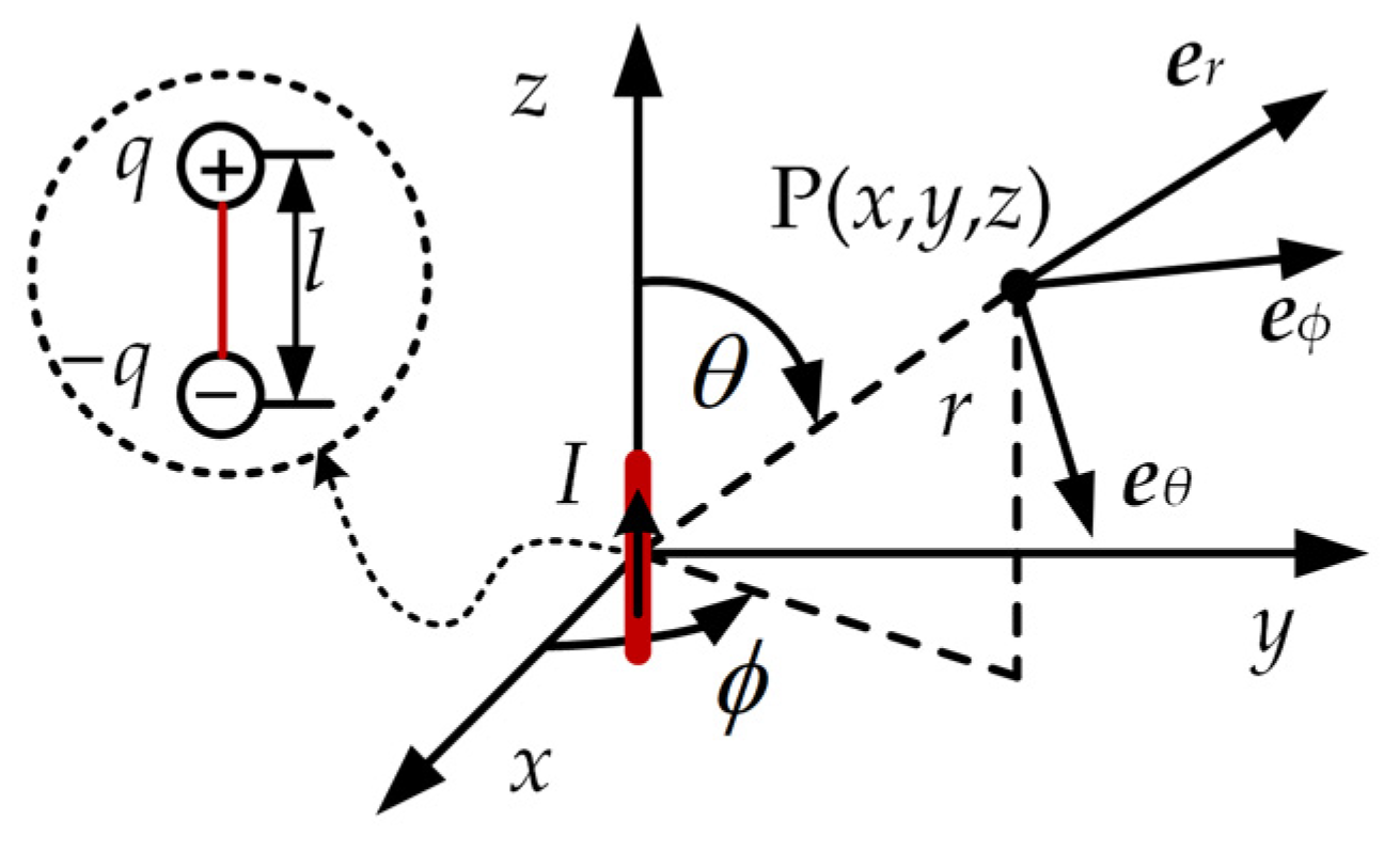
3.1. Equivalent Magnetic Dipole Array Model

The establishment of a planar equivalent magnetic dipole array model is used as an example in this section, and Figure 2 illustrates the relative positions of the computation plane, the magnetic dipole array plane, and the near-field measurement plane. To make better use of the characteristics of near-field measurement data, the magnetic dipole plane corresponding to the near-field measurement plane is divided into the same three regions according to the second Ⅱ, and more magnetic dipoles are set in region A.

In this article, the radiation source is equivalent to a magnetic dipole array through the equivalent dipole method. Each magnetic dipole in the array has a magnetic dipole moment component in the x, y, and z directions, named Mx, My, and Mz.

The radiation magnetic field of a magnetic dipole can be obtained from the electric radiation field of an electric dipole via the dual relationship between an electric dipole and a magnetic dipole [22]. Firstly, the electric radiation field of an electric dipole in free space is solved. Assume that the linear element is l in length, centered at the origin of the rectangular coordinate system, and placed along the z-axis. Let the current on the electric dipole be $i\left(t\right)=\mathit{Icos}\omega t=\mathit{Re}\left[I{e}^{j\omega t}\right]$, which is shown in Figure 3.

Let point P in free space be the coordinate (x, y, z), and the vector magnetic potential of the electric dipole element at point P be A. It is shown in Equation (3).

$$\mathit{A}=\frac{{\mu }_0}{4\pi }{\displaystyle \underset{V}{\mathbf{\int }}\frac{\mathit{J}(\mathit{r}\mathbf{\prime })}{\left|{\mathit{r}}_1-\mathit{r}\mathbf{\prime }\right|}}{e}^{-j{k}_0\left|{\mathit{r}}_1-\mathit{r}\mathbf{\prime }\right|}\mathit{dv}$$

(3)

where V is the integration region, μ₀ is the permeability of the vacuum, dv is the integration element, r′ is the coordinate vector of current density J(r′), and r₁ is the coordinate vector of point P. k₀ represents the wave number in the free space.

According to the symmetry of the coordinates in the coordinate system, when the expression of the z component is found, the expressions of the x and y components can be derived in the same way. In this article, we choose to solve the electric field of the electric dipole moment of z component P_z. The vector magnetic potential A of the z component A_z can be obtained by decomposing Equation (3). Moreover, because the electric dipole is located at the origin of the coordinates and l << r, an approximate expression for the vector magnetic potential A_z can be obtained in Equation (4).

$${\mathit{A}}_{\mathit{z}}=\frac{{\mu }_0}{4\pi }{\mathit{e}}_{\mathit{z}}{\displaystyle \underset{l}{\mathbf{\int }}\frac{I}{r_1}}{e}^{-j{k}_0{r}_1}\mathit{dl}\prime =\frac{{\mu }_0\mathit{Il}}{4\pi r_1}{e}^{-j{k}_0{r}_1}{\mathit{e}}_{\mathit{z}}$$

(4)

According to the principle of electromagnetic fields, a relationship exists between the electric radiation field and the vector magnetic potential of the electric dipole [22], as shown in Equation (5).

$${\mathit{E}}^{\mathit{e}}=\frac{1}{j\omega {\epsilon }_0}\nabla \times (\frac{1}{{\mu }_0}\nabla \times {\mathit{A}}_{\mathit{z}})$$

(5)

where ε₀ is the permittivity of the vacuum. Assume that the electric dipole moment of the z-axis electric dipole is P_z = Il. The electric radiation field of the electric dipole is shown in Equation (6).

$$\{\begin{array}{l}{E}_x^e=\frac{-j{k}_0{\eta }_0}{4\pi }{P}_z\frac{\mathit{xz}}{r_1^2}\left[\frac{3}{{\left(k_0{r}_1\right)}^2}+j\frac{3}{k_0{r}_1}-1\right]\frac{e^{-j{k}_0{r}_1}}{r_1}\hfill \\ E_y^e=\frac{-j{k}_0{\eta }_0}{4\pi r^3}{P}_z\frac{\mathit{yz}}{r_1^2}\left[\frac{3}{{\left(k_0{r}_1\right)}^2}+j\frac{3}{k_0{r}_1}-1\right]\frac{e^{-j{k}_0{r}_1}}{r_1}\hfill \\ E_z^e=-\frac{-j{k}_0{\eta }_0}{4\pi }{P}_z\frac{x^2+y^2}{r_1^2}\left[\frac{3}{{\left(k_0{r}_1\right)}^2}+j\frac{3}{k_0{r}_1}-1\right]\frac{e^{-j{k}_0{r}_1}}{r_1}+\frac{-j{k}_0{\eta }_0}{4\pi }{P}_z\left[\frac{2}{{\left(k_0{r}_1\right)}^2}+j\frac{2}{k_0{r}_1}\right]\frac{e^{-j{k}_0{r}_1}}{r_1}\hfill \end{array}$$

(6)

where η₀ is the wave impedance in free space. The electric field E^e of an electric dipole and the magnetic field H of a magnetic dipole have a dual relationship [22,23]. Therefore, the relationship between the z-direction magnetic dipole Mz and its radiated magnetic field is given by Equation (7). The relation between the magnetic dipole moments Mx and My and the radiation magnetic fields can be deduced by using the symmetry of each component of the rectangular coordinate system. Moreover, the relationship between a magnetic dipole array and its magnetic field can be obtained by using the superposition principle.

$$\{\begin{array}{l}{H}_x=\frac{k_0{}^2}{4\pi }{M}_z\frac{\mathit{xz}}{r_1{}^2}\left[\frac{3}{{\left(k_0{r}_1\right)}^2}+j\frac{3}{k_0{r}_1}-1\right]\frac{e^{-j{k}_0{r}_1}}{r_1}\hfill \\ H_y=\frac{k_0{}^2}{4\pi }{M}_z\frac{\mathit{yz}}{r_1{}^2}\left[\frac{3}{{\left(k_0{r}_1\right)}^2}+j\frac{3}{k_0{r}_1}-1\right]\frac{e^{-j{k}_0{r}_1}}{r_1}\hfill \\ H_z=-\frac{k_0{}^2}{4\pi }{M}_z\frac{x^2+z^2}{r_1}\left[\frac{3}{{\left(k_0{r}_1\right)}^2}+j\frac{3}{k_0{r}_1}-1\right]\frac{e^{-j{k}_0{r}_1}}{r_1}+\frac{k_0{}^2}{4\pi }{M}_z\left[\frac{2}{{\left(k_0{r}_1\right)}^2}+j\frac{2}{k_0{r}_1}\right]\frac{e^{-j{k}_0{r}_1}}{r_1}\hfill \end{array}$$

(7)

where Mz represents the magnetic dipole moment. Hx, Hy, and Hz are the magnetic field intensities of the magnetic field in the x-, y-, and z-directions, respectively. j represents the imaginary unit. $(x_0,y_0,z_0)$ is the coordinate of the magnetic dipole in the z-direction. $(x_1,y_1,z_1)$ is the coordinate of any point in the radiation field of a magnetic dipole. The expression of r₁ is shown in (8).

$$r_1=\sqrt{{(x-x_1)}^2+{(y-y_1)}^2+{(z-z_1)}^2}$$

(8)

If the near-field test data contains phase data, there is a definite relationship between the magnetic dipole array to be solved and the near-field magnetic field, which can be written as a matrix, as shown in (9).

$$\left(\begin{array}{ccc}\left[T_{x,x}\right]& \left[T_{y,x}\right]& \left[T_{z,x}\right]\\ \left[T_{x,y}\right]& \left[T_{y,y}\right]& \left[T_{z,y}\right]\\ \left[T_{x,z}\right]& \left[T_{y,z}\right]& \left[T_{z,z}\right]\end{array}\right)\left(\begin{array}{c}[M_x]\\ [M_y]\\ [M_z]\end{array}\right)=\left(\begin{array}{c}[H_x]\\ [H_y]\\ [H_z]\end{array}\right)$$

(9)

where [Mx], [My], and [Mz] are the magnetic dipole moments of each component of a magnetic dipole in a magnetic dipole array, which is to be solved. The right side of (9), [Hx], [Hy], and [Hz] are known magnetic field intensities, measured by the near field. The calculation formula of coefficient matrix T is shown in (10).

$$\{\begin{array}{l}{T}_{x,x}=-\frac{k_0^2}{4\pi }\left[{(y_p^{\prime }-y_p)}^2+{(z_p^{\prime }-z_p)}^2\right]\left[\frac{3}{{\left(k_{0}r\right)}^2}+j\frac{3}{k_{0}r}-1\right]\frac{e^{-j{k}_{0}r}}{r^3}+\frac{k_0^2}{4\pi }\left[\frac{2}{{\left(k_{0}r\right)}^2}+j\frac{2}{k_{0}r}\right]\frac{e^{-j{k}_{0}r}}{r}\hfill \\ T_{y,x}=\frac{k_0^2}{4\pi }\left[(x_p^{\prime }-x_p)\times (y_p^{\prime }-y_p)\right]\left[\frac{3}{{\left(k_{0}r\right)}^2}+j\frac{3}{k_{0}r}-1\right]\frac{e^{-j{k}_{0}r}}{r^3}\hfill \\ T_{z,x}=\frac{k_0^2}{4\pi }\left[(x_p^{\prime }-x_p)\times (z_p^{\prime }-z_p)\right]\left[\frac{3}{{\left(k_{0}r\right)}^2}+j\frac{3}{k_{0}r}-1\right]\frac{e^{-j{k}_{0}r}}{r^3}\hfill \\ T_{x,y}=\frac{k_0^2}{4\pi }\left[(x_p^{\prime }-x_p)\times (y_p^{\prime }-y_p)\right]\left[\frac{3}{{\left(k_{0}r\right)}^2}+j\frac{3}{k_{0}r}-1\right]\frac{e^{-j{k}_{0}r}}{r^3}\hfill \\ T_{y,y}=-\frac{k_0^2}{4\pi }\left[{(x_p^{\prime }-x_p)}^2+{(z_p^{\prime }-z_p)}^2\right]\left[\frac{3}{{\left(k_{0}r\right)}^2}+j\frac{3}{k_{0}r}-1\right]\frac{e^{-j{k}_{0}r}}{r^3}+\frac{k_0^2}{4\pi }\left[\frac{2}{{\left(k_{0}r\right)}^2}+j\frac{2}{k_{0}r}\right]\frac{e^{-j{k}_{0}r}}{r}\hfill \\ T_{z,y}=\frac{k_0^2}{4\pi }\left[(y_p^{\prime }-y_p)\times (z_p^{\prime }-z_p)\right]\left[\frac{3}{{\left(k_{0}r\right)}^2}+j\frac{3}{k_{0}r}-1\right]\frac{e^{-j{k}_{0}r}}{r^3}\hfill \\ T_{x,z}=\frac{k_0^2}{4\pi }\left[(x_p^{\prime }-x_p)\times (z_p^{\prime }-z_p)\right]\left[\frac{3}{{\left(k_{0}r\right)}^2}+j\frac{3}{k_{0}r}-1\right]\frac{e^{-j{k}_{0}r}}{r^3}\hfill \\ T_{y,z}=\frac{k_0^2}{4\pi }\left[(y_p^{\prime }-y_p)\times (z_p^{\prime }-z_p)\right]\left[\frac{3}{{\left(k_{0}r\right)}^2}+j\frac{3}{k_{0}r}-1\right]\frac{e^{-j{k}_{0}r}}{r^3}\hfill \\ T_{z,z}=-\frac{k_0^2}{4\pi }\left[{(x_p^{\prime }-x_p)}^2+{(y_p^{\prime }-y_p)}^2\right]\left[\frac{3}{{\left(k_{0}r\right)}^2}+j\frac{3}{k_{0}r}-1\right]\frac{e^{-j{k}_{0}r}}{r^3}+\frac{k_0^2}{4\pi }\left[\frac{2}{{\left(k_{0}r\right)}^2}+j\frac{2}{k_{0}r}\right]\frac{e^{-j{k}_{0}r}}{r}\hfill \end{array}$$

(10)

r is the distance between the magnetic dipole which coordinate is $(x_p^{\prime },y_p^{\prime },z_p^{\prime })$ and the measuring point which coordinate is $(x_i,y_i,z_i)$, p = 1, 2, …, M, M is the total number of magnetic dipoles; i = 1, 2, …, N, N is the total number of measuring points. The position of each magnetic dipole is randomly selected in its own region. The expression of r is shown in (11).

$$r=\sqrt{{(x_p^{\prime }-x_i)}^2+{(y_p^{\prime }-y_i)}^2+{(z_p^{\prime }-z_i)}^2}$$

(11)

If the near-field measurement data do not contain phase data, there is no definite relationship between the magnetic dipole array and the near-field magnetic field, so it becomes an optimization problem. This article uses differential evolution algorithms in [24,25] to solve this problem.

The differential evolution algorithm was proposed by Kenneth V.P. and Storn R. in 1997 to solve optimization problems [25]. The differential evolution algorithm was proposed for minimizing non-linear functions, and it is a simple and efficient meta-heuristic algorithm for solving for global optimal solutions. The algorithm continues the search with the best vectors through mutation and selection operations to obtain an optimal solution.

Firstly, the initial population $\left\{X_{g,t,0}=(x_{g,1,0},x_{g,2,0},\dots ,x_{g,\mathit{NP},0})|t=1,2,\dots ,\mathit{NP}\right\}$ is randomly generated according to a uniform distribution $x_g^{low}\le x_{g,t,0}\le x_g^{up}$, for g = 1, 2, …, D, where D is the dimension of the problem and D = 6. NP is the population size. The expression of an individual in a population is Equation (12).

$$x_{g,t,0}=\left\{\mathit{Re}\left(M_x\right),\mathit{Im}\left(M_x\right),\mathit{Re}\left(M_y\right),\mathit{Im}\left(M_y\right),\mathit{Re}\left(M_z\right),\mathit{Im}\left(M_z\right)\right\}$$

(12)

where Re is the real part of the magnetic dipole moment and Im is the imaginary part of the magnetic dipole moment.

The fitness value of the initial population is computed by (13). The relative error expression in (13) is used as the fitness function, similar to [24].

$$f={\displaystyle \sum _{i=1}^N{\displaystyle \sum _{t=x,y,z}\sqrt{\frac{{(\mathit{Re}(H_{t,i}^{\mathit{calc}})-\mathit{Re}(H_{t,i}^{\mathit{sim}}))}^2+{(\mathit{Im}(H_{t,i}^{\mathit{calc}})-\mathit{Im}(H_{t,i}^{\mathit{sim}}))}^2}{\mathit{Re}{(H_{t,i}^{\mathit{sim}})}^2+\mathit{Im}{(H_{t,i}^{\mathit{sim}})}^2}}}}$$

(13)

$H_{t,i}^{\mathit{calc}}$ is the magnetic field intensity calculated by the magnetic dipole array through Equation (9) and $H_{t,i}^{\mathit{sim}}$ is the known magnetic field intensity.

Following that, mutation and crossover operation will produce a new generation of magnetic dipole arrays with each iteration [25]. The mutation vector V_g,t,i is obtained from Equation (14).

$${\mathit{V}}_{g,t,G}={\mathit{X}}_{g,\mathit{best},G}+F\times ({\mathit{X}}_{g,r1,G}-{\mathit{X}}_{g,r2,G})$$

(14)

X_g,r1,G − X_g,r2,G is a difference vector to mutate the corresponding parent X_g,G. X_g,best,G is the best vector at the current generation G. F is the mutation factor which usually ranges on the interval (0, 2).

The crossover vector U_g,t,i is obtained from Equation (15) [25].

$${\mathit{U}}_{g,t,G}=\{\begin{array}{l}{\mathit{V}}_{g,t,G}, \mathrm{if} \mathit{CR}\le \mathrm{rand}(0,1) \mathrm{or} j=j_{\mathit{rand}}\hfill \\ {\mathit{X}}_{g,t,G}, \mathrm{otherwise}\hfill \end{array}$$

(15)

where CR is the crossover factor which usually ranges on the interval (0, 1). j_rand = randint(1, D) is an integer randomly chosen from 1 to D and newly generated for each t.

Finally, the best array is chosen by contrasting the fitness values of the magnetic dipole arrays from the previous and new generations. The selection operation is based on Formula (16) [25].

$${\mathit{X}}_{g,t,G+1}=\{\begin{array}{l}{\mathit{U}}_{g,t,G}, \mathrm{if} f({\mathit{U}}_{g,t,G})\le f({\mathit{X}}_{g,t,G})\hfill \\ {\mathit{X}}_{g,t,G}, \mathrm{otherwise}\hfill \end{array}$$

(16)

Repeat the above steps until the best magnetic dipole array is obtained. The process of the equivalent dipole method based on the differential evolution algorithm is shown in Figure 4.

3.2. The Solution of Ill-Conditioned Matrix

It is challenging to directly obtain a stable solution since the coefficient matrix in (9) has a large condition number, making it an ill-conditioned matrix. In this article, the least square method and Tikhonov regularization are used to solve (9). For the convenience of discussion, (9) can be abbreviated as TM = H.

Tikhonov regularization corrects the error of the quantity by adding a regularization parameter so that the solution result of an ill-conditioned matrix is a stable approximate solution. The form of the least square method combined with Tikhonov regularization is shown in (17).

$$\min {\Vert \mathit{TM}-\mathit{H}\Vert }^2+{\lambda }^2{\Vert \mathit{M}\Vert }^2$$

(17)

where λ is the regularization parameter which is unknown. The solution of (13) by Tikhonov regularization is (18). (T)^T is the transposed matrix of T.

$$\mathit{M}={\left({\left(\mathit{T}\right)}^{\mathit{T}}\mathit{T}+{\lambda }^2\mathit{I}\right)}^{-1}{\left(\mathit{T}\right)}^{\mathit{T}}\mathit{H}$$

(18)

where I is a 3M × 3M identity matrix.

In this article, generalized cross-validation (GCV) [26] is used to solve the regularization parameter because it has a wide range of applications. The theory of GCV is to divide the right-hand side H of Equation (9) into two parts, with one part being used to solve the approximate solution and the other part being used to verify the approximate solution so as to obtain a suitable regularization parameter.

$${\mathit{M}}_{\lambda }^{\left(\mathit{t}\right)}={\left[\right({\mathit{T}}^{(\mathit{t})}{)}^T{\mathit{T}}^{\left(\mathit{t}\right)}+{\lambda }^2\mathit{I}]}^{-1}{({\mathit{T}}^{(\mathit{t})})}^T{\mathit{H}}^{\left(\mathit{t}\right)}$$

(19)

where H^(t) is the vector obtained by deleting the element H_t of H, T^(t) is the matrix obtained by deleting the t-the row of T. As shown in (19), the deleted element H_t can be calculated by ${\mathit{T}}^{\left(t\right)}{\mathit{M}}_{\lambda }^{\left(t\right)}$. A suitable regularization parameter λ can minimize the error of all elements.

When Equation (19) is minimized, λ is the solution required by Equation (20).

$$\min {\left(\frac{m\Vert {\mathit{H}}^{\left(t\right)}-{\mathit{T}}^{\left(t\right)}{\mathit{M}}_{\lambda }^{\left(t\right)}\Vert }{m-\mathit{trace}\left(\mathit{T}{\left({\mathit{T}}^T\mathit{T}+{\lambda }^2\mathit{I}\right)}^{-1}{\mathit{T}}^T\right)}\right)}^2$$

(20)

where m is the number of the part that is used to solve the approximate solution.

4. Experiment and Simulation Verification

According to the measurement method based on the field distribution characteristics proposed in the previous section, in this section, an experiment and a simulation example are used to verify that the measurement method can greatly reduce the amount of near-field measurement data and improve the equivalent modeling efficiency of low-frequency radiation from powerful electromagnetic equipment while ensuring the accuracy of radiation source modeling.

4.1. Experiment Verification

In order to verify the measurement and modeling methods presented in this article, experiments are first carried out to simulate low-frequency radiation interference generated by powerful electromagnetic equipment. The sinusoidal signal with a frequency of 60 Hz and a peak-to-peak value of 2 V is added to the low-frequency ring antenna through the frequency characteristic module. The antenna is then placed inside an aluminum casing that has apertures. The test scene is shown in Figure 5.

A three-axis fluxgate sensor and magnetic effect measurement system was used to measure the magnetic fields of two surfaces with lengths ranging from −35 cm to 50 cm and widths ranging from −50 cm to 50 cm. The two surfaces are 7.5 cm and 12.5 cm away from the radiation source, respectively. The plane at 7.5 cm away from the radiation source is the measurement plane, and the plane at 12.5 cm away from the radiation source is the calculation plane. The magnetic field distribution of the calculation plane obtained from the measurement data is shown in Figure 6.

First, the measurement plane was measured by sparse and uniform sampling, and the sampling interval was 2 cm. A total of 51*43 = 2193 measurement points were obtained. Then, the DE algorithm is used to solve the magnetic dipole array model composed of 36 magnetic dipoles uniformly arranged. The magnetic field intensity calculated by the equivalent magnetic dipole array and the measurement value of the calculation plane’s magnetic field intensity compute the relative error of the magnetic field intensity through (9). The relative errors are shown in

Table 1. Relative error of the magnetic field is obtained when 2193 data is used.

Magnetic-Field Component	Hx	Hy	Hz	H
Relative error of amplitude	22.88%	23.74%	23.86%	23.11%

.

Secondly, the test method proposed in this article was used to obtain near-field data with a large sampling interval of 5 cm through sparse and uniform sampling. After that, the magnetic field intensity of additional measuring points was measured according to the measurement method. Total near-field data increased from 378 to 423, and the distribution of measurement points is shown in Figure 7. The area surrounded by the green line is area A, the area surrounded by the blue and green lines is area B, and the remaining part is area C. The black dots are the locations of sparse and uniform sampling, and the red dots are the positions of the additional measuring points.

According to Section 2, the near-field data obtained by the measurement method and the DE algorithm are used to solve the radiation source equivalent model of the magnetic dipole array composed of 36 magnetic dipoles. The values of the real and imaginary parts of the magnetic dipole moment obtained by the equivalent dipole method and the DE algorithm are shown in Figure 8.

This model was used to calculate the magnetic field intensity in the calculation plane, as shown in Figure 9.

The magnetic field intensity calculated by the equivalent magnetic dipole array and the measurement value of the calculation plane’s magnetic field intensity compute the relative error of the magnetic field intensity through (9). The relative errors are shown in

Table 2. Relative errors of magnetic field obtained by method of this article.

Magnetic-Field Component	Hx	Hy	Hz	H
Relative error of amplitude	23.75%	25.18%	25.27%	24.34%

.

As can be seen from Figure 9, the distribution of the magnetic field intensity obtained by the proposed method is consistent with the experimental results. At the same time, it can be seen from Table 2 that when the amount of near-field measurement data is reduced by five times, the relative error obtained by this method is also small. In addition, due to the smaller amount of data used in each iteration of the DE algorithm, the calculation is faster, and the preset fitness value can be reached faster. The modeling time required by this method is 287.48 s, which is 4.2 times less than that required by uniform sampling. This shows that the method of near-field measurement and equivalent modeling of radiation characteristics based on near-field distribution characteristics can greatly reduce the amount of near-field data required for modeling and improve the efficiency of the modeling while achieving the required accuracy of modeling.

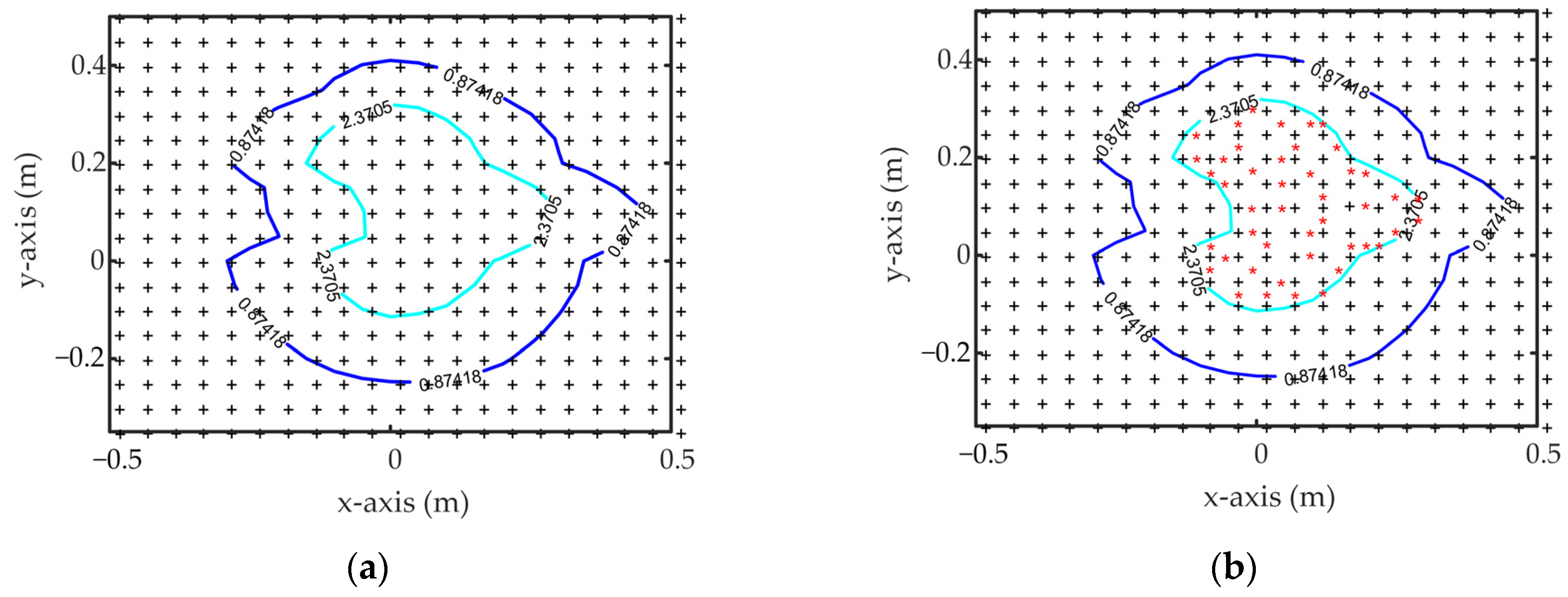
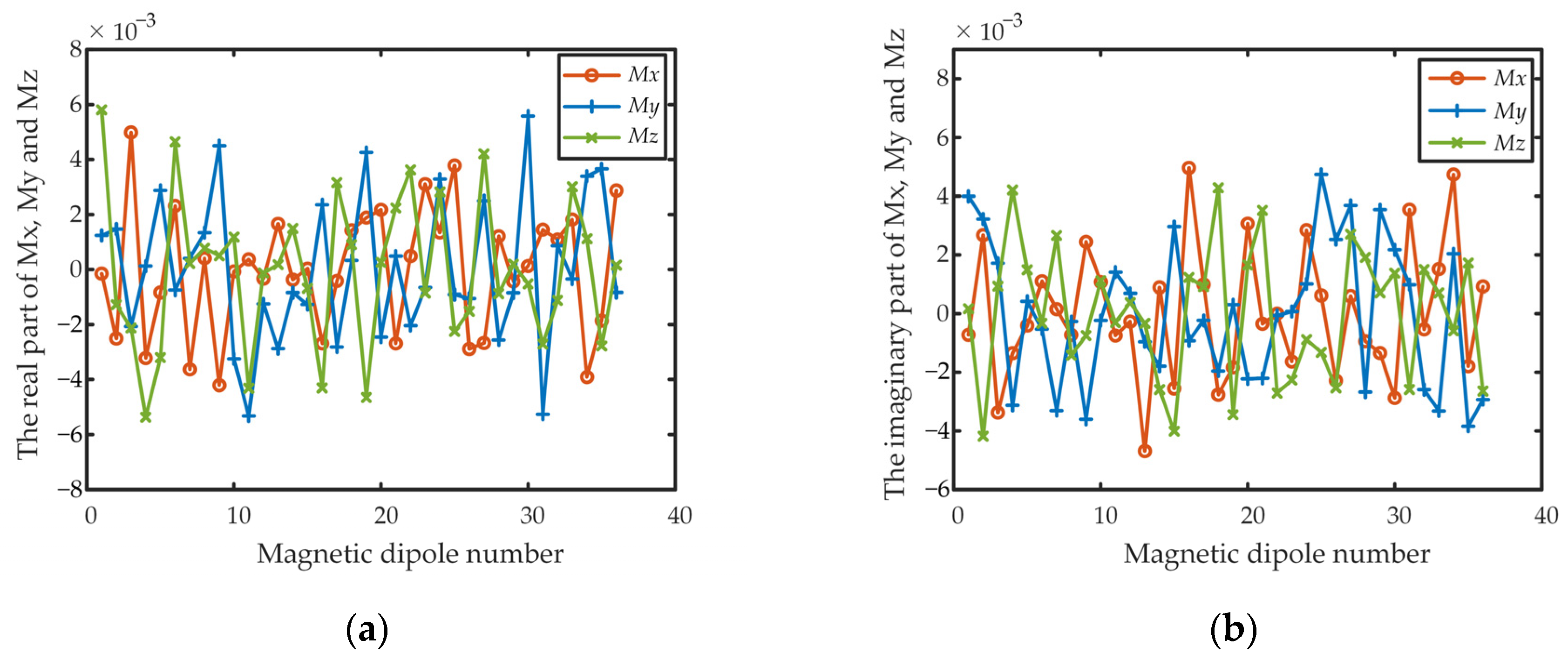
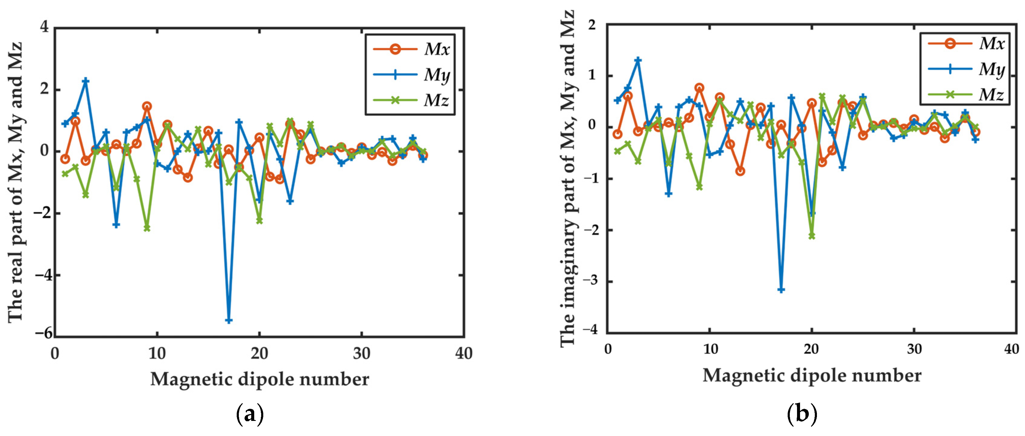
4.2. Simulation Verification

The model of a powerful electromagnetic equipment cabinet was established in the three-dimensional full-wave electromagnetic simulation software Maxwell3D, as shown in Figure 10. The near-field amplitude and phase data obtained with simulation are used as validation data for the test method proposed in this article. The model consists of three little cabinets that are 1.60 m long, 1.20 m wide, and 2.4 m high, respectively. Three coils are arranged in the three cabinets to serve as radiation sources. The currents flowing through each coil are 1∠30° kA, 1∠25° kA, and 1∠45° kA, respectively. The frequency of the three coils is 60 Hz.

The dimensions of the measuring plane, magnetic dipole array plane, and calculation plane are 2.8 m × 2.8 m, and the distance from the cabinet is 0.1 m, 0.05 m, and 0.4 m, respectively. The magnetic field distribution of the calculation plane obtained by Maxwell3D simulation is shown in Figure 11.

To verify the modeling effect of the near-field measurement and the equivalent modeling of radiation characteristics based on near-field distribution characteristics when reducing the amount of near-field data, firstly, select the sampling points with an interval of 4 cm to measure the measuring plane; a total of 71*71 = 5041 measuring points are obtained. Then, a magnetic dipole array radiation source model composed of 36 magnetic dipoles with a uniform distribution is obtained by using the near-field data.

The magnetic field intensity calculated by the equivalent magnetic dipole array and the measurement value of the calculation plane’s magnetic field intensity compute the relative error of the magnetic field intensity through (9). The relative errors are shown in

Table 3. Relative error of the magnetic field is obtained when 2193 data are used.

Magnetic-Field Component	Hx	Hy	Hz	H
Relative error of amplitude	1.44%	2.62%	2.14%	1.52%
Relative error of phase	17.36%	21.26%	14.29%	10.64%

.

The measurement method proposed in this article is used to collect near-field data with a large sampling interval of 15 cm through sparse and uniform sampling. Then, the magnetic field of the additional measuring points is measured according to the measurement method. The number of near-field data points increased from 361 to 451. The distribution of measurement points is shown in Figure 12.

The near-field data collected by the measurement method were used to create the magnetic dipole array model, which consists of 36 magnetic dipoles. The values of the real and imaginary parts of the magnetic dipole moment obtained by the equivalent dipole method are shown in Figure 13.

The magnetic field distribution of the calculation plane was calculated using this model, as shown in Figure 14.

The magnetic field intensity calculated by the equivalent magnetic dipole array and the measurement value of the calculation plane’s magnetic field intensity compute the relative error of the magnetic field intensity through (9). The relative errors are shown in

Table 4. Relative errors of magnetic field obtained by method of this article.

Magnetic-Field Component	Hx	Hy	Hz	H
Relative error of amplitude	1.99%	3.63%	3.47%	2.02%
Relative error of phase	16.24%	18.33%	15.23%	9.77%

.

As can be seen from Figure 14, the amplitude distribution and phase distribution obtained by the equivalent magnetic dipole array are consistent with the simulation results. At the same time, it can be seen from Table 4 that when the amount of near-field data is reduced by 11 times, the relative error calculated by the method in this article is also small. Meanwhile, the modeling time required by this method is 7.323 s, which is 2.5 times less than that required by uniform sampling. This demonstrates that the approach of near-field measurement and equivalent modeling of radiation characteristics based on near-field distribution characteristics can significantly reduce the amount of near-field data needed for equivalent radiation modeling and enhance the modeling’s efficiency.

5. Conclusions

In order to solve the problems of large amounts of near-field data, long testing times, and low modeling efficiency in the equivalent modeling of low-frequency radiation characteristics of powerful electromagnetic equipment, this article proposes a method of near-field measurement and equivalent modeling of the radiation characteristics of powerful electromagnetic equipment based on field distribution characteristics. First, sparse and uniform sampling with large sample intervals is used to collect the near-field data, and then the distribution features of the near-field are obtained by using the near-field data. Then, the total near-field data is obtained by further measurement in the area with a large magnetic field amplitude. The simulation and experiment show that the near-field data can be reduced to 1/5 or even better under the condition of ensuring the modeling accuracy, which greatly improves the modeling efficiency. This method can be applied to the equivalent modeling of the radiation characteristics of a variety of large-scale, powerful electromagnetic equipment, supporting low-frequency electromagnetic environment prediction and electromagnetic compatibility design on various platforms.

References

1. Gharib, A.; Griffiths, H.D.; Andrews, D.J. Prediction of Topside Electromagnetic Compatibility in Concept-Phase Ship Design. IEEE Trans. Electromagn. Compat. 2017, 59, 67–76. [Google Scholar] [CrossRef]
2. Georgiou, C.D.; Kalaitzopoulou, E.; Skipitari, M.; Papadea, P.; Varemmenou, A.; Gavriil, V.; Sarantopoulou, E.; Kollia, Z.; Cefalas, A.-C. Physical Differences between Man-Made and Cosmic Microwave Electromagnetic Radiation and Their Exposure Limits, and Radiofrequencies as Generators of Biotoxic Free Radicals. Radiation 2022, 2, 285–302. [Google Scholar] [CrossRef]
3. Zhao, Y.; Baharuddin, M.D.; Smartt, C.; Zhao, X.; Yan, L.P.; Liu, C.J.; Thomas, D.W.P. Measurement of Near-Field Electromagnetic Emissions and Characterization Based on Equivalent Dipole Model in Time-Domain. IEEE Trans. Electromagn. Compat. 2020, 62, 1237–1246. [Google Scholar] [CrossRef]
4. Song, T.-H.; Wei, X.-C.; Tang, Z.-Y.; Gao, R.X.-K. Broadband Radiation Source Reconstruction Based on Phaseless Magnetic Near-Field Scanning. IEEE Antennas Wirel. Propag. Lett. 2021, 20, 113–117. [Google Scholar] [CrossRef]
5. Yan, Z.W.; Wang, J.W.; Zhang, W.; Wang, Y.S.; Fan, J. A Simple Miniature Ultrawideband Magnetic Field Probe Design for Magnetic Near-Field Measurements. IEEE Trans. Antennas Propag. 2016, 64, 5459–5465. [Google Scholar] [CrossRef]
6. Zhang, J.C.; Wei, X.C.; Yang, R.; Gao, R.X.K.; Yang, Y.B. An Efficient Probe Calibration Based Near-Field-to-Near-Field Transformation for EMI Diagnosis. IEEE Trans. Antennas Propag. 2019, 67, 4141–4147. [Google Scholar] [CrossRef]
7. Serpaud, S.; Boyer, A.; Dhia, S.B.; Coccetti, F. Efficiency of Sequential Spatial Adaptive Sampling Algorithm to Accelerate Multifrequency Near-Field Scanning Measurement. IEEE Trans. Electromagn. Compat. 2022, 64, 816–826. [Google Scholar] [CrossRef]
8. Shao, W.H.; Fang, W.X.; Huang, Y.; Li, G.W.; Wang, L.; He, Z.Y.; Shao, E.; Guo, Y.D.; En, Y.F.; Yao, B. Simultaneous Measurement of Electric and Magnetic Fields with a Dual Probe for Efficient Near-Field Scanning. IEEE Trans. Antennas Propag. 2019, 67, 2859–2864. [Google Scholar] [CrossRef]
9. Huangfu, Y.P.; Wang, S.H.; Rienzo, L.D.; Zhu, J.G. Radiated EMI Modeling and Performance Analysis of a PWM PMSM Drive System Based on Field-Circuit Coupled FEM. IEEE Trans. Magn. 2017, 53, 1–4. [Google Scholar] [CrossRef]
10. Shinde, S.; Masuda, K.; Shen, G.Y.; Patnaik, A.; Makharashvili, T.; Pommerenke, D.; Khilkevich, V. Radiated EMI Estimation from DC–DC Converters with Attached Cables based on Terminal Equivalent Circuit Modeling. IEEE Trans. Electromagn. Compat. 2018, 60, 1769–1776. [Google Scholar] [CrossRef]
11. Zhang, Y.; Lu, J.; Pacheco, J.; Moss, C.D.; Ao, C.O.; Grzegorczyk, T.M.; Kong, J.A. Mode-Expansion Method for Calculating Electromagnetic Waves Scattered by Objects on Rough Ocean Surfaces. IEEE Trans. Antennas Propag. 2005, 53, 1631–1639. [Google Scholar] [CrossRef]
12. Solis, D.M.; Martín, V.F.; Araujo, M.G.; Larios, D.; Obelleiro, F.; Taboada, J.M. Accurate EMC Engineering on Realistic Platforms Using an Integral Equation Domain Decomposition Approach. IEEE Trans. Antennas Propag. 2020, 68, 3002–3015. [Google Scholar] [CrossRef]
13. Sarkar, T.K.; Taaghol, A. Near-Field to Near/Far-Field Transformation for Arbitrary Near-Field Geometry Utilizing an Equivalent Electric Current and MoM. IEEE Trans. Antennas Propag. 1999, 47, 566–573. [Google Scholar] [CrossRef]
14. Baharin, R.H.M.; Omi, S.; Uno, T.; Arima, T. Internal Electric Field Reconstruction and SAR Estimation of In-Body Antenna Using Inverse Equivalent Current Method. IEEE Trans. Electromagn. Compat. 2021, 63, 1658–1666. [Google Scholar] [CrossRef]
15. Shu, Y.F.; Wei, X.C.; Fan, J.; Yang, R.; Yang, Y.B. An Equivalent Dipole Model Hybrid with Artificial Neural Network for Electromagnetic Interference Prediction. IRE Trans. Microwave Theory Tech. 2019, 67, 1790–1797. [Google Scholar] [CrossRef]
16. Zhang, J.; Pommerenke, D.; Fan, J. Determining Equivalent Dipoles Using a Hybrid Source-Reconstruction Method for Characterizing Emissions from Integrated Circuits. IEEE Trans. Electromagn. Compat. 2017, 59, 567–575. [Google Scholar] [CrossRef]
17. Jin, H.H.; Wang, H.; Zhuang, Z.H. A New Simple Method to Design Degaussing Coils Using Magnetic Dipoles. J. Mar. Sci. Eng. 2022, 10, 1495–1512. [Google Scholar] [CrossRef]
18. Wen, J.; Ding, L.; Zhang, Y.L.; Wei, X.C. Equivalent Electromagnetic Hybrid Dipole Based on Cascade-Forward Neural Network to Predict Near-Field Magnitude of Complex Environmental Radiation. IEEE J. Multiscale Multiphys. Comput. Techn. 2020, 5, 227–234. [Google Scholar] [CrossRef]
19. Zhang, J.; Fan, J. Source Reconstruction for IC Radiated Emissions based on Magnitude-only Near-Field Scanning. IEEE Trans. Electromagn. Compat. 2017, 59, 557–566. [Google Scholar] [CrossRef]
20. Shu, Y.F.; Wei, X.C.; Yang, R.; Liu, E.X. An Iterative Approach for EMI Source Reconstruction Based on Phaseless and Single-Plane Near-Field Scanning. IEEE Trans. Electromagn. Compat. 2018, 60, 937–944. [Google Scholar] [CrossRef]
21. Sørensen, M.; Franek, O.; Pedersen, G.F.; Radchenko, A.; Kam, K.; Pommerenke, D. Estimate on the Uncertainty of Predicting Radiated Emission from Near-Field Scan Caused by Insufficient or Inaccurate Near-Field Data: Evaluation of the Needed Step Size, Phase Accuracy and the Need for All Surfaces in the Huygens’ Box. In Proceedings of the International Symposium on Electromagnetic Compatibility-EMC EUROPE, Rome, Italy, 17–21 September 2012; pp. 1–6. [Google Scholar]
22. Wilson, P. On Correlating TEM Cell and OATS Emission Measurements. IEEE Trans. Electromagn. Compat. 1995, 37, 1–16. [Google Scholar] [CrossRef]
23. Obiekezie, C.K.; Thomas, D.W.P.; Nothofer, A.; Greedy, S.; Arnaut, L.R.; Sewell, P. Complex Locations of Equivalent Dipoles for Improved Characterization of Radiated Emissions. IEEE Trans. Electromagn. Compat. 2014, 56, 1087–1094. [Google Scholar] [CrossRef]
24. Wang, B.F.; Liu, X.A.; Zhao, W.J.; Png, C.E. Reconstruction of Equivalent Emission Sources for PCBs from Near-Field Scanning Using a Differential Evolution Algorithm. IEEE Trans. Electromagn. Compat. 2018, 60, 1670–1677. [Google Scholar] [CrossRef]
25. Storn, R.; Price, K. Differential Evolution-A Simple and Efficient Heuristic for Global Optimization over Continuous Spaces. J. Glob. Optimt. 1997, 11, 341–359. [Google Scholar] [CrossRef]
26. Xu, P. Iterative Generalized Cross-Validation for Fusing Heteroscedastic Data of Inverse Ill-Posed Problems. Geophys. J. Int. 2009, 179, 182–200. [Google Scholar] [CrossRef] [Green Version]
Figure 1. Schematic diagram of measurement method based on near-field distribution characteristics (a) Sparse uniform sampling; (b) Divide areas according to magnetic field intensity; (c) Calculate the magnetic field change for each point in region A. αq is shown in Equation (1).; (d) Additional measurement. d, √2d, and 0.5√2d are the distances between the corresponding two points.
Energies 16 02005 g001
Figure 2. Schematic diagram of the equivalent dipole method. Compared with the near-field measurement plane, the magnetic dipole array plane is divided into three zones: A, B and C.
Energies 16 02005 g002
Figure 3. Schematic diagram of an electric dipole.
Energies 16 02005 g003
Figure 4. The process of equivalent dipole method based on the differential evolution algorithm.
Energies 16 02005 g004
Figure 5. Test scene.
Energies 16 02005 g005
Figure 6. The distribution of magnetic field intensity at 12.5 cm away from the radiation source. (a) The amplitude distribution of H; (b) The amplitude distribution of Hx; (c) The amplitude distribution of Hy; (d) The amplitude distribution of Hz.
Energies 16 02005 g006
Figure 7. The distribution of measuring points. (a) Before the additional measurement; (b) After the additional measurement.
Energies 16 02005 g007
Figure 8. The values of the real and imaginary parts of the magnetic dipole moment. (a) The values of the real part of the magnetic dipole moment; (b) The values of the imaginary part of the magnetic dipole moment.
Energies 16 02005 g008
Figure 9. The distribution of magnetic field intensity is calculated by the equivalent magnetic dipole array. (a) The amplitude distribution of H; (b) The amplitude distribution of Hx; (c) The amplitude distribution of Hy; (d) The amplitude distribution of Hz.
Energies 16 02005 g009
Figure 10. Electronic cabinet model in the Maxwell3D.
Energies 16 02005 g010
Figure 11. The distribution of the magnetic field which is calculated by the simulation model. (a) The amplitude distribution of H; (b) The amplitude distribution of Hx; (c) The amplitude distribution of Hy; (d) The amplitude distribution of Hz; (e) The phase distribution of H; (f) The phase distribution of Hx; (g) The phase distribution of Hy; (h) The phase distribution of Hz.
Energies 16 02005 g011
Figure 12. The distribution of measuring points. (a) Before the additional measurement; (b) After the additional measurement.
Energies 16 02005 g012
Figure 13. The values of the real and imaginary parts of the magnetic dipole moment. (a) The values of the real part of the magnetic dipole moment; (b) The values of the imaginary part of the magnetic dipole moment.
Energies 16 02005 g013
Figure 14. The distribution of the magnetic field calculated by the equivalent magnetic dipole array. (a) The amplitude distribution of H; (b) The amplitude distribution of Hx; (c) The amplitude distribution of Hy; (d) The amplitude distribution of Hz; (e) The phase distribution of H; (f) The phase distribution of Hx; (g) The phase distribution of Hy; (h) The phase distribution of Hz.
Energies 16 02005 g014