Numerical Simulation Study of Huff-n-Puff Hydrocarbon Gas Injection Parameters for Enhanced Shale Oil Recovery

Abstract

Gas injection has already proven to be an efficient shale oil recovery method successfully tested all around the world. However, gas-enhanced oil recovery methods have never been implemented or tested for the greatest Siberian shale oil formation yet. This article proposes numerical simulation of a hydrocarbon gas injection process into a horizontal well with multiple hydraulic fractures perforating Bazhenov shale oil formation in Western Siberia characterized by ultra-low permeability. A complex field-scale numerical study of gas injection for such a formation has never been performed before and is presented for the first time in our work. The hydrodynamic compositional simulation was performed utilizing a commercial simulator. A sensitivity study for different operating parameters including cycle times, bottom-hole pressures for the production and injection period, and injected gas composition was performed after the model was history matched with the available production data. Some uncertain reservoir properties such as relative permeability curves were also sensitized upon. Two different ways of accounting for multiple hydraulic fractures in the simulation model are presented and the simulation results from both models are compared and discussed. Eventually, huff-n-puff injection of a hydrocarbon gas resulted in a 34–117% increase in oil recovery depending on the fracture model.

1. Introduction

Gas injection (both miscible and immiscible hydrocarbon gas or CO₂) is one of the most efficient enhanced oil recovery (EOR) methods for conventional oil reservoirs worldwide and accounted for 56% of enhanced oil recovery projects worldwide in 2017 [1]. The revolution in shale oil development over the past decade has led to extensive research into applicable EOR for such deposits, and various studies have reported the potential of miscible gas injection to enhance oil recovery in organic-rich shale [2]. Typically, these reservoirs are developed by primary depletion through horizontal wells with multi-stage hydraulic fracturing. This technology greatly improves communication within the reservoir, allowing the reservoir to displace crude oil primarily through rock and fluid expansion. The main difficulty in the development of shale oil and gas fields is low reservoir properties, such as porosity and permeability, and high oil saturation of about 95–98%. For example, the Middle Bakken shale oil reservoir has a porosity of about 7% and a permeability of less than 0.05 mD [3], while the Barnett shale gas field has a porosity of about 5% and an average permeability of about 30 nD [4]. Similar formations in the Eagle Ford field have a porosity of about 10% and a permeability ranging from 5 to 800 nD [5], while the Duvernay Shale in Canada has a porosity of about 6% and a permeability of about 0.4 nD [6]. These reservoirs are also developed by creating multiple transverse fractures—multiple hydraulic fracturing. At the moment, the world’s leading companies are searching for the optimal technology for the development of such reservoirs. If we consider fluid injection, the injectivity in injection wells would be close to zero due to poor filtration properties, so gas injection seems to be the most viable method for developing shale formations. Gas injection as a method of secondary oil recovery, which has been successfully applied in traditional reservoirs for many years, such as the Tengiz oil field in Kazakhstan [7], the Provincia field in Colombia [8], and others, has shown prospects for additional oil production. A lot of research has been carried out recently to improve our understanding of the processes that occur when gas is injected into shale reservoirs. A comprehensive review of research before 2020 is presented by [9]. According to the conducted analysis of published studies and based on earlier publications [10], cyclic injection or huff-n-puff (HNP) injection seems to be much better suited for shale oil reservoirs. During HNP, the well briefly serves as an injector, after which it produces hydrocarbons for a period of time (instead of the more traditional method that involves a dedicated injector and producer) and then switches back to injection, effectively stimulating the reservoir volume around the well [11]. The method consists of three steps. The injection step—gas is injected into the reservoir through fractures in a horizontal well; the impregnation/soaking step—the well is shut in and gas is allowed to enter the shale matrix through hydraulic and natural fractures; and the production step—the reservoir is depressurized and the well is put back into production, allowing oil to expand from the source.

The methodology used to study the effectiveness of using associated gas as an enhanced oil recovery method can be divided into two categories: laboratory experiments on core plugs and numerical simulations. Most core experiments show very promising results in terms of enhanced oil recovery, while simulation studies are less encouraging as they show almost no additional oil recovery from gas HNP [12,13]. This difference is due to several factors. Firstly, most laboratory studies conducted in this area of research have used synthetic oils and outcrop cores, which cannot fully reflect the nanopores of shale media and reservoir fluids [14]. Secondly, there are many questions about the simulation results, ranging from the chosen grid sizes to the applicability of Darcy’s law alone to fluid transport through an organic shale matrix [15]. There have been several studies reporting the results of pilot applications of gas huff-n-puff methods, such as the article on HNP CO₂ pilot projects in the Bakken [16] and gas HNP in the Eagle Ford Shale [17,18]. The authors used publicly available data, and although they could not clearly see an increase in oil production for some of the prototypes, those where this analysis was carried out showed an increase in oil production.

Recently, several studies have been published that have primarily focused on optimizing gas injection modes in the huff stage and gas production modes in the puff stage. One such interesting work is the patent developed by James J. Sheng [19]. In general, the invention features a method to enhance oil recovery in shale reservoirs using a huff-n-puff gas injection process that includes a plurality of huff periods and a plurality of puff periods. The method includes the step of determining a maximum injection rate and a maximum injection pressure to be used during the plurality of huff periods. The method further includes the step of determining the maximum gas flow rate, the maximum oil production rate, and the minimum production pressure from the well during the plurality of puff periods. The method further includes the step of setting a huff period time for the plurality of huff periods such that the pressure the near wellbore reaches the determined maximum injection pressure during the huff period.

This paper is dedicated to the study of the associated petroleum gas injection in the huff-n-puff mode in terms of optimizing the modes based on the numerical simulation of the Bazhenov formation of one of the West Siberian oil fields.

Bazhenov is a unique oil shale formation in Western Siberia characterized by exceptional petrophysical and geological properties which makes it different from any other oil shale formation in the world. The organic matter of the Bazhenov formation is represented by kerogen embedded in the rock matrix of different lithotypes, hydrocarbons bound to the rock surface or kerogen [20], and mobile oil and gas. The lithotypes are finely distributed within the thin-layered formation making it a source rock, a reservoir, and a seal at the same time. A low thickness (50 m on average), complex pore structure and geology, absence of nearby aquifers or initial water saturation, abnormally high reservoir pressure in some production wells, and uneven distribution of reservoir properties unrelated to lithological parameters [21] define the formation throughout the whole 1 mln sq. km area.

Petrophysical studies of core samples from the Bazhenov formation of various fields have shown the presence of porous-fractured and fractured reservoirs, which are characterized, first of all, by a strong variability of reservoir properties over the area of the suite. Most formations have low porosity (1–2%) and permeability of less than 5 µD [22]. However, in the sections of some wells, there are interlayers with a porosity coefficient reaching 16%. At the moment, the Bazhenov deposits are being developed mainly for depletion; however, leading companies in the country are conducting research to find the most effective technology for developing these deposits. In this study, we used compositional reservoir simulation to understand the feasibility and applicability of cyclic gas injection into the Bazhenov shale, an organic-rich formation in Western Siberia characterized by ultra-low permeability [23]. A sector model containing a single horizontal well with multi-stage hydraulic fractures was matched to the available production data and then used to optimize the operating parameters of cyclic injection of hydrocarbon gas. The optimal scenario was then subjected to uncertainty evaluation by changing some uncertain parameters, the choice of which will be described below. The key research in this work is the search for the optimal mode without the soaking effect, which in turn reduces the time to achieve the effect.

The purpose of this article is to study the influence of some key parameters on the results of the tuned hydrodynamic model and to create reliable production forecasts for the Bazhenov formation. A complex numerical study of gas injection for such a reservoir has never been performed before and is presented for the first time in our work. The published studies presenting simulations of cyclic gas (CO₂ or hydrocarbon gas) injection [6,24,25] included the following list of uncertain parameters: fracture characteristics (pseudo-crack width), reservoir (e.g., absolute and relative permeability, water saturation, average formation pressure, matrix porosity, and Kv/Kn ratio), fluid type (different compositions with different values of minimum mixing pressure (MMP)), and the presence of natural cracks. Several authors have reported their approach to molecular diffusion modeling for CO₂ and gaseous HNP processes, but analysis of the simulation results showed that it requires large computational costs and does not affect the performance of gaseous HNP [25], so it was not included in our simulation model. In our opinion, MMR was the most important parameter for this process, and it was important to obtain reliable estimates. Initially, we used empirical correlations (based on [10]) but later conducted a series of simulations using thin tubes to determine this value for the initial composition of the hydrocarbon gas and the compositions selected as sensitivity parameters.

2. Materials and Methods

2.1. Simulation Model Set-Up and Parameters Description

The sector model around the well was cut down from the original full-field model. The simulation grid was modified in order to better account for existing hydraulic fractures. The orientation of hydraulic fractures was assumed to be perpendicular to the horizontal wellbore. The areal grid was made non-uniform with the thinnest cells close to the fracture plane and the cell size in the X direction was increased from 0.1 to 5 m. The cell sizes in the Y direction were kept uniform and equal to 5 m (Figure 1). The main properties of the model are shown in

Table 1. Properties of the model.

Parameters	Values
Grid dimension	175 × 38 × 38
Number of active cells	98,673
Average permeability, mD	0.23
Average porosity, %	7
Type of model	Compositional/5 components
Oil density at standard conditions, kg/m3	827
Oil viscosity at reservoir conditions, cP	0.36
Initial reservoir temperature, deg C	95
Initial oil saturation, %	98
Initial reservoir pressure, bar	234
Saturation pressure, MPa	140.5

.

In this paper, the history was adapted from the start of oil production, followed by hydraulic fracturing, to the start of the huff-n-puff gas process. The main methods of model history matching are fracture parameters such as length, opening, and height, as well as the area near the fracture (SRV zone) where the reservoir properties are expected to increase, leading to reservoir damage due to hydraulic fracturing [26,27]. The fracture length varied from 50 to 250 m, the height varied from 5 to 25 m, the SRV zone varied from 1 to 4 m, and the crack opening varied from 1 to 5 mm. The fracture permeability was set to 17 mD. Thus, the fracture height was 25 m, the fracture length was 200 m, the fracture aperture was 3 mm, the SRV zone was determined to be 3 m, and the permeability in the SRV zone was given exponentially and was distributed from 8.5 to 0.23 mD from the fracture zone. The permeability of the matrix did not change.

The comparison of the calculated development indicators with the observed data is shown in Figure 2.

More details about the reservoir’s properties, simulation model, and approach can be found in [23].

There was an ncertainty about the presence of natural fractures in the Bazhenov formation even though they were not detected during well-logging. The decision was made to simulate two reservoir models: model A, where hydraulic fractures do not connect with the natural fracture network, and model B, where the natural fracture network is activated during the hydraulic fracturing process; dual porosity region in the vicinity of hydraulic fractures are introduced in order to account for stimulated reservoir volume (SRV).

The PVT model was based on available downhole fluid sample laboratory test data and the results of the swelling test. The three-parameter Peng Robinson equation of state was adjusted for the differential liberation test results, matching the initial GOR and saturation pressure and the swelling test results. The lab report contained a fluid description down to C13+, and the components were grouped into five pseudo-components for easy simulation,

Table 2. The reservoir oil and injection gas compositions used the in simulation.

Pseudo Components	Reservoir Oil (Base), %mol	Injected Gas (Base), %mol
N2 + C1	34.88	60.34
C2 + CO2	10.15	17.58
C3-C4	13.3	20.48
C5-C7	10.94	1.6
C8+	30.74	0

. The composition of the injected gas in the simulation is set on the basis of the composition of associated gas in the field, produced from other productive formations in this field.

The investigated well started to produce oil from the Bazhenov formation after nine-stage hydraulic fracturing was performed. The production history with measurements of oil, water, gas flow rates, and bottomhole pressures (BHP) for the first three following years was available to perform the history match and reduce some of the uncertainties. The main history matching parameters for model A were the absolute reservoir permeability distribution, hydraulic fracture parameters (fracture conductivity and absolute permeability), and the transmissibility between the oil-bearing formation and the underlying water-saturated horizon. Production data for the after-fracking period showed that there was a possibility for the fractures to break the barrier between these two formations. For model B, the additional parameters were the porosity and permeability of natural fractures and the relative permeability curves in fractures and the matrix.

2.2. Calculation of Forecast Variants Using Huff-n-Puff Technology

The base case scenario was a depletion strategy after fracturing. The HNP gas injection process was implemented in the model shortly after fracturing [18]. This was completed so as to avoid the reservoir pressure dropping below the estimated MMP value.

Several operating parameters were varied to define the optimum injection strategy: the bottom hole pressure for the injection (BHPinj) and production (BHPprod) cycle and the length of each cycle: injection/soak period/production [19]. The ranges of the sensitivity parameters, as well as the resulting cumulative oil production for 5 years, are presented in

Table 3. Simulated scenarios and results for models A and B.

Case	BHP Inj, Atm	BHP Prod, Atm	Inj Cycle Length, Months	Soak Cycle Length, Months	Prod Cycle Length, Months	Cum. Oil Production, m3
						Model A	Model B
0	-	50	-	-	-	1100	1105
1	300	250	1	0	1	706	853
2			1	0	2	645	718
3			2	0	1	622	703
4			1	0	5	644	655
5	300	150	1	0	1	1404	2345
6			1	0	2	1291	2337
7			2	0	1	1186	1930
8			1	0	5	1080	1878
9			1	1	2	1064	1830
10			1	1	4	1032	1818
11	300	100	1	0	1	1477	2809
12			1	0	2	1351	2767
13			2	0	1	1262	2391
14			1	0	5	1158	2206
15			1	1	2	1123	2285
16			1	1	4	1115	2175
17	300	50	1	0	1	1367	3056
18			1	0	2	1184	2894
19			2	0	1	1167	2681
20			1	0	5	1041	2194
21			1	1	2	1013	2559
22			1	1	4	924	2209

, where production is reported for one fracture. To obtain an estimate of oil production for the whole well, the numbers need to be multiplied by nine. The choice of the injection bottom hole pressure was determined by two facts: the value of minimum miscibility pressure for hydrocarbon gas of 225 atm and the known value of fracture initiation pressure of 340 atm. The production pressure range was chosen to see the effect of miscibility. The MMP value was 225 atm, so at a maximum production pressure of 250 atm, we were expecting to have a miscible process. The maximum injection pressure of 300 atm was selected in order to achieve miscibility and to avoid the creation of extra fractures because the fracturing pressure was 340 atm.

For each of the fracture models (A and B), the optimal combination of operating parameters was determined to ensure a maximum cumulative oil production value after 5 years. For model A, the maximum cumulative oil was reached for the following combination of parameters: BHPinj = 300 bar, BHPprod = 100 bar, and six injection cycles per year (1 month of injection followed directly by 1 month of production). An additional 34% of oil was produced in comparison to the depletion process (1477 m³ vs. 1100 m³ in the case of a one-fracture region). For model B, the maximum cumulative oil was reached at BHPinj = 300 bar, BHPprod = 50 bar, and six injection cycles per year (1 month of injection followed directly by 1 month of production), Table 3. An additional 177% of oil was produced in comparison to the depletion process (3056 m³ vs. 1105 m³ in the case of a 1-fracture region).

It was surprising to find that the length of the soaking period did not affect the cumulative oil production, and the best results were for the cases without soaking. A possible explanation for this fact is the absence of diffusion or adsorption effects in the simulation model. At the time of the study, the authors did not have any lab data on these parameters; hence, it was decided to leave them out of the investigation.

In order to estimate how uncertainties in the miscibility pressure and relative permeability curves affect the implementation of the huff-n-puff gas injection process as an EOR method, simple sensitivity studies for these parameters were conducted for optimum production scenarios on both simulation models (A and B).

2.3. Diffusion Modeling Methods

One of the most important studies of gas injection into a reservoir is the study of diffusion and its effect on cumulative oil production. Diffusion is the mutual penetration of particles of one substance between particles of another, while their concentrations are spontaneously aligned throughout the occupied volume. Previously, this value was not taken into account in the calculations presented; however, to show the degree of influence of diffusion in our opinion is a necessary aspect.

Let us consider a mathematical model of diffusion implemented in the tNavigator simulator (Technical User’s Guide). tNavigator implements a model of molecular diffusion caused by a concentration gradient. In the general case, the flow of matter of the i-th component through a unit area per unit time is written as:

$$Q_i=-c·D_i·\nabla x_i$$

(1)

where c is the total molar concentration, calculated as c = 1/ν_m, kg-mol/rm³; ν_m is the molar volume of the mixture; D_i is the diffusion coefficient of the ith component, m²/day; ∇ = ∂/∂d is the gradient in the direction of the flow; and x_i is the mole fraction of the ith component.

In addition to diffusion within a single phase (gas or oil), diffusion between phases must also be taken into account. In tNavigator, the problem of interfacial diffusion is reduced to the problem of diffusion within one phase. An artificial buffer zone, shown schematically in Figure 3, is created at the boundary between adjacent blocks. It is assumed that fluids mix in this zone and the composition of the mixture is the result of mixing the compositions in these blocks. The resulting composition is used to determine the molecular diffusion potential for each component. The molar flux of a component between phases is the diffusive flux of that component through the buffer zone within the same phase. If the concentration of the component in the block is greater than its value in the buffer zone, then it is considered that the component flowing into the buffer zone for one phase has diffused into another phase.

Let us consider two blocks, I and J, containing oil and gas, respectively. The composition in the buffer zone is calculated as:

$${\tilde{m}}_i={\left({\xi }_0·x_i\right)}_j+{\left({\xi }_g·y_i\right)}_j$$

(2)

where ξ_o is the molar density of the oil phase; x_i is the mole fraction of oil of the i-th component; ξ_g is the molar density of the gas phase; and y_i is the mole fraction of the i-th component gas.

The temperature and pressure in the buffer zone are assumed to be half the sum of the temperatures and pressures in the blocks:

$$\tilde{P}=\frac{P_i+P_j}{2},\hspace{1em}\hspace{1em}\tilde{T}=\frac{T_i+T_j}{2} .$$

(3)

Let ${\tilde{x}}_i$ and ${\tilde{y}}_i$ be the molar fractions of the components in the oil and gas phase in the buffer zone and let ${\tilde{\xi }}_o$ and ${\tilde{\xi }}_g$ be their molar densities, respectively. As an example, let us consider the case: x_i > ${\tilde{x}}_i$ and y_i > ${\tilde{y}}_i$, then two diffusion flows of component I will arise: from the oil phase to the gas phase FX_og and from the gas phase to the oil phase FY_go (Figure 3). FX_og is the component flow from block I to the buffer zone within the oil phase. FY_go is the component flow from block J to the buffer zone within the gas phase. The diffusion flow between oil in block I and gas in block J for the i-th component is calculated as:

F = FX_og + FY_go,

(4)

$${\mathrm{FX}}_{\mathrm{og}}=\mathrm{Di}\mathrm{f}\mathrm{f}·{\mathrm{D}}_{\mathrm{ogi}}·\min ({\mathrm{S}}_{\mathrm{oI}},{\mathrm{S}}_{\mathrm{gJ}})·{\mathsf{\xi }}_{\mathrm{O}}·(\mathrm{x}{\mathrm{i}}_{}-{\tilde{x}}_i)$$

(5)

$${\mathrm{FY}}_{\mathrm{go}}=\mathrm{Di}\mathrm{f}\mathrm{f}·{\mathrm{D}}_{\mathrm{goi}}·\min ({\mathrm{S}}_{\mathrm{oI}},{\mathrm{S}}_{\mathrm{gJ}})·{\mathsf{\xi }}_{\mathrm{G}}·(\mathrm{x}{\mathrm{i}}_{}-{\tilde{x}}_i)$$

(6)

where S_I and S_J are the saturation of oil and gas, respectively; Di f f is diffuseness; and D_ogi and D_goi are diffusion coefficients between the oil–gas phases, m²/day.

3. Results

3.1. Variations for Model A

3.1.1. Relative Permeability Curves

The available data were obtained in a laboratory using core samples from the Bazhenov formation. One set of curves was used for all of the cells except for the hydraulic fracture cells, where straight lines were used. However, it is a well-known fact that shale oil reservoirs are highly heterogeneous, and we need to assume some uncertainty here. That is why some endpoints in the oil–gas system were changed to see the effect on oil production, see Figure 4 and

Table 4. Relative permeability curve sets.

Original Set			RP1			RP2
Sg, Fraction	Krg, Fraction	Krog, Fraction	Sg, Fraction	Krg, Fraction	Krog, Fraction	Sg, Fraction	Krg, Fraction	Krog, Fraction
0	0	1	0	0	1	0	0	1
0.023	0.01	0.581	0.021	0.01	0.581	0.062	0.01	0.581
0.052	0.02	0.314	0.046	0.02	0.314	0.139	0.02	0.314
0.097	0.03	0.109	0.087	0.03	0.109	0.259	0.03	0.109
0.142	0.05	0.039	0.127	0.05	0.039	0.380	0.05	0.039
0.157	0.07	0.027	0.142	0.07	0.027	0.426	0.07	0.027
0.195	0.12	0.011	0.174	0.12	0.011	0.522	0.12	0.011
0.224	0.17	0	0.2	0.17	0	0.6	0.17	0

.

The resulting change in cumulative oil production can be seen in Figure 5. As expected, an increase in SOGCR (RP2) leads to an increase in cumulative oil production after 5 years (7.8% in comparison to the base value) and even a slight decrease in SOGCR (RP1) results in a 9% decrease in 5-year cumulative oil production.

3.1.2. Minimum Miscibility Pressure

Since we cannot control the MMP value, which is often one of the most uncertain parameters for the gas injection process, we studied the sensitivity to this parameter by injecting a composition with a higher or lower MMP than was determined for our produced gas. In all cases, the MMP value was estimated by numerical simulation of slimtube experiments.

Table 5. MMP values for different injected compositions.

	HC Gas Injection	Methane Injection	Ethane/Propane Injection
MMP, bar	225	500	110

contains the MMP values for two extra compositions of injected gas. In the minimum scenario, pure methane was injected; in the maximum scenario—a mixture of 80% ethane and 20% propane–butane.

As can be seen in Figure 6, the injected gas composition plays a very important role in the displacement process. Non-miscible oil displacement in the minimum scenario decreases cumulative oil production by 72% compared to the base scenario and fully miscible displacement allows for the cumulative oil recovery to increase by 49%.

3.2. Comparison of Model A and Model B Simulation Results

A sensitivity study for the displacement type was also conducted on model B (SRV model), with the same variations in injected gas composition. The results were similar to the model A results with a significant increase of 33.5% in the maximum scenario and a 68% decrease in the minimum scenario.

It is also important to compare the simulation results for two fracture models. This was carried out using an optimum production scenario for each method of fracture representation. As can be seen in Figure 7, model B (SRV) predicts much higher gas HNP performance than model A. This can be explained by an increase in the contact area added by the natural fractures’ presence and more chances for pure mixing and swelling between the injected gas and reservoir fluids, resulting in substantial additional oil recovery.

4. Comparison of Development Indicators When Choosing Components of a Compositional Oil Model

To reduce the calculation time, a study was carried on a number of the components’ influence on the main development indicators, such as cumulative oil and gas production, reservoir pressure, and the dynamics of production of the gas component composition. For this purpose, compositional models consisting of five, eight, and nine pseudo components were considered, and the compositions of the associated injected gas were calculated (

Table 6. Formation oil and injected gas compositions.

5-Pseudo Components	Reservoir Oil (Base), %mol	Injected Gas (Base), %mol	8-Pseudo Components	Reservoir Oil (Base), %mol	Injected Gas (Base), %mol	9-Pseudo Components	Reservoir Oil (Base), %mol	Injected Gas (Base), %mol
N2 + C1	34.87	60.34	N2 + C1	34.87	60.34	CO2	0.89	1.7
C2 + CO2	10.15	17.58	CO2 + C2 + C3	20.79	22.7	N2 + C1	34.87	60.34
C3 + C4	13.3	20.48	iC4 + nC4	5.41	15.36	C2 + C3	19.9	21
C5 + C7	10.94	1.6	iC5 + nC5 + C6	4.55	1.3	iC4 + nC4	5.41	15.36
C8+	30.74	0	C7 + C8 + C9	14.6	0.3	iC5 + nC5 + C6	4.55	1.3
			C10-C13	7.63	0	C7 + C8 + C9	14.6	0.3
			C14-C20	8.26	0	C10-C13	7.63	0
			C21-C29	3.89	0	C14-C20	8.26	0
						C21-C29	3.89	0

).

The main idea behind this approach is that models with a high number of components have a long computation time and tend to have problems with the convergence of the equations at the time step. Oil production and associated gas injection modes were selected using a five-component model, which made it possible to evaluate the effect of the huff-n-puff technology for a large number of modes. This study made it possible to select the optimal component composition of oil and the resulting optimal modes were calculated accordingly on the optimal compositional model. A comparison of the calculation results is shown in Figure 8 and Figure 9.

The results obtained show an almost two-fold increase in oil production when using a model with eight and nine components compared to a 5-component model, and a three-fold increase in gas production, with virtually no differences over the period of adaptation. Moreover, the production decline rates when using a five-component model are lower compared to multi-component ones. At the same time, the differences between the eight-component model and the nine-component one, where CO₂ is isolated as a separate component, are minimal, which indicates that it is optimal to use the eight-component model for further studies.

The distribution at the same time step of the main molar fraction of the N₂ + C₁ component for all three (five-, eight-, and nine-component) models is shown in Figure 10.

Figure 10 shows that the 60.34% component in the main component composition N₂ + C₁ of the injected associated gas increases the degree of sweep by the gas reservoir.

5. Influence of Diffusion on Development Parameters

This model uses experimentally determined average diffusion coefficients of associated gas in the free volume, in the artificial core, and for the matrix of the Bazhenov formation. For the purpose of studying the influence, for simplification, the diffusion coefficients for the free volume are taken as for the fracture zone, the diffusion coefficients in the artificial core are taken as coefficients for the SRV zone, and the diffusion coefficients for the Bazhenov core—as for the matrix, see the values in

Table 7. Results of model calculations with different diffusion coefficients.

Model Name	Diffusion Coefficient, m2/day	Cumulative Oil Production, m3	Error between the Model without Diffusion, %
Without diffusion		1973	-
Diffusion for fracture zone	0.00685152	2040	3.40
Diffusion for SRV	0.00011059	1972	−0.05
Diffusion for matrix	0.00002471	1939	1.72

. Due to the limited scope of experimental studies, the diffusion coefficients for each component are constant.

The results of cumulative oil production and pressure dynamics for the selected optimal model in terms of modes are shown in Figure 11, Figure 12 and Figure 13.

The obtained results of calculations showed a negligible effect of diffusion both on the cumulative oil production and on such development indicators as the dynamics of oil production and reservoir pressures compared to the model without diffusion. A detailed review of the obtained deviations is presented in Table 7.

According to the results obtained, the largest deviations from the model, which does not take into account diffusion, are observed for the coefficients obtained in the free volume. This value corresponds to the fracture zone; however, the main oil inflow comes from the SRV zone. Therefore, in our opinion, for the model that most realistically describes the inflow to the well, it is better to use diffusion values obtained experimentally for an artificial core. However, as we can see from Table 7, the results differ by no more than 0.05% compared to the case without diffusion. Even if we consider the results obtained for the diffusion coefficients on the Bazhenov core (see the diffusion for the matrix model), the difference in the cumulative oil production is less than 2%. Thus, it can be concluded that for the simulated problem statement, the influence of diffusion processes is minimal, but at the same time, the calculation time of the model increases significantly, and this factor can be neglected. Thorough research on diffusion processes during hydrocarbon gas injection in the huff-n-puff mode and a definition of diffusion coefficients for each component may change this perception.

6. Discussion and Conclusions

As we see from the simulation, the huff-n-puff gas injection process is an effective method to increase oil recovery from Bazhenov oil shales. The efficiency of the method depends both on geological factors and on the selected mode. In this work, a fairly large scatter in the increment of cumulative oil production was obtained, which can be affected by the limitations adopted in the model.

The main limitations in this work are primarily geological: distributions of permeability, porosity, and lithology, which are obtained using a statistical distribution. Due to the fact that the Bazhenov formation is very heterogeneous in terms of reservoir characteristics, this point can introduce errors in determining the cumulative oil production in the implementation of any technology, including huff-n-puff. In addition, PVT models are based on a recombined sample, not a reservoir sample, since a reservoir sample has not been taken for this formation at the moment. However, even in this case, we expect errors, since there is a proven non-uniformity in the distribution of temperatures and saturation pressures for similar reservoirs in other fields in Western Siberia. This factor will also affect the permafrost if we consider another well of this formation. If we consider the diffusion parameters, then the diffusion coefficients of the associated gas components in the reservoir oil gas released at the stage of reservoir oil degassing in the development process have not been obtained. For the sake of simplicity, they are set an order of magnitude higher than the diffusion coefficients of associated gas in reservoir oil. In addition, finally, if we consider the diffusion coefficients for individual components as a whole, then the same values are given for each component due to the fact that these experiments were not performed experimentally. All of these factors in total will introduce an error into the obtained simulation results; however, in general, qualitatively performed calculations are sufficient for making decisions about the effectiveness of the method and the optimality of the selected modes.

A study on the effect of the number of components showed an almost two-fold increase in oil production for the case with more detailed fluid composition, which indicates that this analysis is required when modeling this technology. At the same time, use of a less detailed model allowed us to perform the best production mode selection faster, due to the optimum run time of this model. In this case, it is necessary to take into account corrections for cumulative production if we simplify the PVT model in order to speed up calculations.

This paper considers the effect of the diffusion coefficient on cumulative oil production. Due to the fact that a simplified diffusion model is given, that is, constant diffusion coefficients for various components are given, we did not acquire significant differences from the model without diffusion. However, it should be borne in mind that with a more detailed approach, it is necessary to take into account the uneven setting of diffusion coefficients depending on the filtration properties of the reservoir. This stage is planned as one of the next research steps. Experts suggest that diffusion is not as important for hydrocarbon gas injection as it is for CO₂ injection [2]; however, the HNP process is not a gas displacement process, so we recommend investigating diffusion effects in detail.

Laboratory MMP measurements on reservoir oil samples with different gas compositions are the most required in order to optimize the displacement mechanism and make it closer to a fully miscible process. In addition, it is necessary to have a wider range of permafrost studies in case the thermobaric properties of the formation change for another well.

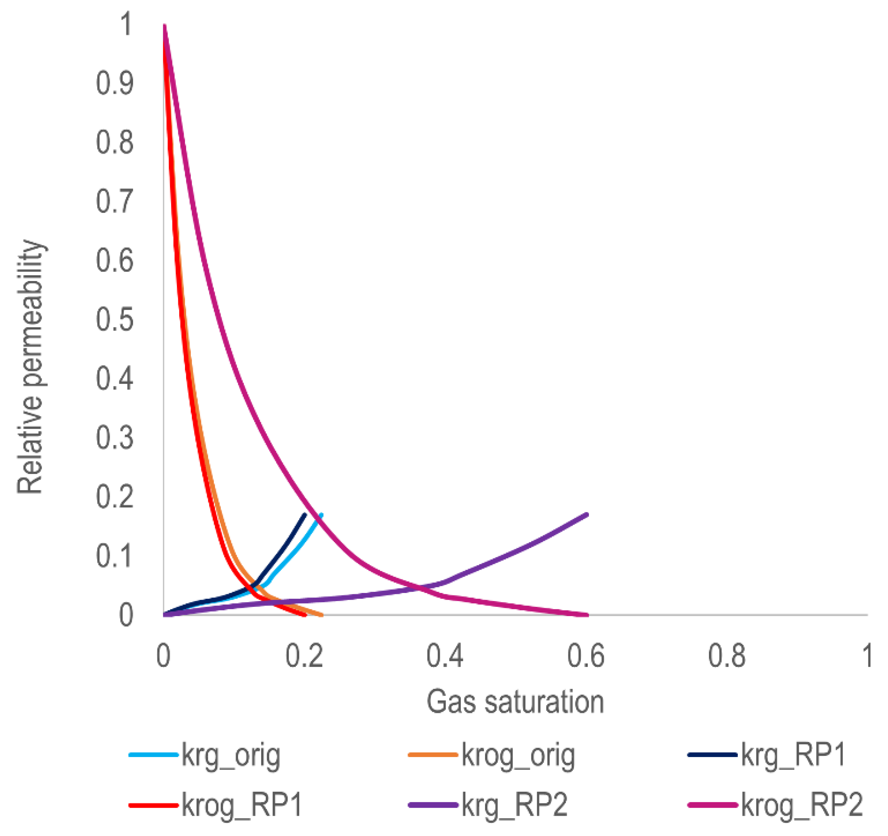
As we have seen, variations in relative permeability endpoints cause a significant difference in the simulation results. Future work should focus on the effects of hysteresis on oil production, as mentioned in [28]. Upscaling methods of relative permeabilities obtained in laboratory experiments are crucial for simulation results and should also be carefully investigated. In general, it would be interesting, as a part of future work, to consider how a change in the HTP model will affect the endpoints of the relative permeability curves. This setting can be carried out on the basis of the performed oil displacement by associated gas experiment in the huff-n-puff mode.

The presented simulation results show how uncertain simulation parameters affect the production forecasts for the gas huff-n-puff process in shale oil formations. Hence, further research is much needed in order to reduce the uncertainties related to this EOR method.

To conclude, the conducted study showed the EOR potential of the huff-n-puff gas injection method for the Bazhenov oil formation and also highlighted how much research is still needed to commercially develop it in the near future.

References

1. McGlade, C.; Sondak, G. Whatever Happened to Enhanced Oil Recovery. 2018. Available online: https://www.iea.org/commentaries/whatever-happened-to-enhanced-oil-recovery (accessed on 5 January 2020).
2. Alfarge, D.; Wei, M.; Bai, B. IOR Methods in Unconventional Reservoirs of North America: Comprehensive Review. In Proceedings of the SPE Western Regional Meeting, Bakersfield, CA, USA, 23–27 April 2017. SPE-185640-MS. [Google Scholar] [CrossRef]
3. Allharthy, N.; Teklu, T.; Kazemi, N.; Graves, R.; Hawthorne, S.; Braunberger, J.; Kurtoglu, B. Enhanced Oil Recovery in Liquid-Rich Shale Reservoirs: Laboratory to Field. In Proceedings of the SPE Annual Technical Conference and Exhibition, Houston, TX, USA, 28–30 September 2015. SPE-175034. [Google Scholar]
4. Cipolla, C.L.; Warpinski, N.R.; Mayerhofer, M.J.; Lolon, E.P. The Relationship between Fracture Complexity, Reservoir Properties, and Fracture-Treatment Design. In Proceedings of the SPE Annual Technical Conferene and Exhibition, Denver, CO, USA, 21–24 September 2010. [Google Scholar]
5. Kosanke, T.H.; Warren, A. Geological Controls on Matrix Permeability of the Eagle Ford Shale (Cretaceous), South Texas, USA. In The Eagle Ford Shale: A Renaissance in U.S. Oil Production; Breyer, J., Ed.; American Association of Petroleum Geologists: Tulsa, OK, USA, 2016. [Google Scholar] [CrossRef]
6. Hamdi, H.; Clarkson, C.R.; Ghanizadeh, A.; Ghaderi, S.M.; Vahedian, A.; Riazi, N.; Esmail, A. Huff-n-Puff Gas Injection Performance in Shale Reservoirs: A Case Study from Duvernay Shale in Alberta, Canada. In Proceedings of the SPE/AAPG/SEG Unconventional Resources Technology Conference, Houston, TX, USA, 23–25 July 2018. URTEC-2902835-MS. [Google Scholar] [CrossRef]
7. Darmentaev, S.; Yessaliyev, A.; Azhigaliyeva, A.; Belanger, D.; Sullivan, M.; King, G.; Feyijime, T.; Bateman, P. Tengiz Sour Gas Injection Project. In Proceedings of the SPE Caspian Carbonates Technology Conference, Atyrau, Kazakhstan, 8–10 November 2010. [Google Scholar]
8. Rivera, J.E.; Duarte, C.A.; Chaparro, C.H.; Fernandez, F.R.; Quinterro, L.M.; Villareal, R.M.; Pinto, J.C.; Sarquez, J.R.; Sachica, J.A.; Amaya, R.F.; et al. Comparison between Cyclic Gas Injection and Cyclic Solvent Plus Gas Injection. In Proceedings of the SPE Latin America and Caribbean Heavy and Heavy Extra Oil Conference held in Lima, Lima, Peru, 9–20 October 2016. [Google Scholar]
9. Burrows, L.C.; Haeri, F.; Cvetic, P.; Sanguinito, S.; Shi, F.; Tapriyal, D.; Goodman, A.; Enick, R.M. A Literature Review of CO2, Natural Gas, and Water-Based Fluids for Enhanced Oil Recovery in Unconventional Reservoirs. Energy Fuels 2020, 34, 5331–5380. [Google Scholar] [CrossRef]
10. Alfarge, D.; Wei, M.; Bai, B.; Alsaba, M. Analysis of IOR Pilots in Bakken Formation by Using Numerical Simulation. In Proceedings of the Abu Dhabi International Petroleum Exhibition & Conference, Abu Dhabi, United Arab Emirates, 13–16 November 2017. SPE-188633-MS. [Google Scholar] [CrossRef]
11. Pankaj, P.; Mukisa, H.; Solovyeva, I.; Xue, H. Enhanced Oil Recovery in Eagle Ford: Opportunities Using Huff-n-Puff Technique in Unconventional Reservoirs. In Proceedings of the SPE Liquids-Rich Basins Niorth Amercia Conference in Midland, Midland, TX, USA, 5–6 September 2018. SPE 191780-MS. [Google Scholar]
12. Gala, D.P.; Sharma, M.M. Compositional and Geomechanical Effects in Huff-n-Puff Gas Injection IOR in Tight Oil Reservoirs. In Proceedings of the SPE Annual Technical Conference and Exhibition in Dallas, Dallas, TX, USA, 24–26 September 2018. SPE-191488-MS. [Google Scholar]
13. Tsau, J.-S.; Fu, Q.; Barati, R.G.; Zaghloul, J.; Baldwin, A.; Bradford, K.; Nicoud, B.; Mohrbacher, J.D. Experimental Investigation of Hydrocarbon Gas Huff-N-Puff Injection into the Live-Oil Window of Eagle Ford. In Proceedings of the Abu Dhabi International Petroleum Exhibition & Conference, Abu Dhabi, United Arab Emirates, 15–18 November 2021. SPE-207224-MS. [Google Scholar] [CrossRef]
14. Alfarge, D.; Alsaba, M.; Wei, M.; Bai, B. Miscible Gases Based EOR in Unconventional Liquids Rich Reservoirs: What We Can Learn. In Proceedings of the SPE International Heavy Oil Conference and Exhibition, Kuwait City, Kuwait, 10–12 December 2018. SPE-193748-MS. [Google Scholar] [CrossRef]
15. Tovar, F.D.; Barrufet, M.A.; Schechter, D.S. Gas Injection for EOR in Organic Rich Shale. Part I: Operational Philosophy. In Proceedings of the SPE Improved Oil Recovery Conference, Tulsa, OK, USA, 14–18 April 2018. SPE-190323-MS. [Google Scholar] [CrossRef]
16. Todd, H.B.; Evans, J.G. Improved Oil Recovery IOR Pilot Projects in the Bakken Formation. In Proceedings of the SPE Low Perm Symposium, Denver, CO, USA, 5–6 May 2016. SPE-180270-MS. [Google Scholar]
17. Todd, H.B. Huff-N-Puff Gas Injection Pilot Projects in the Eagle Ford. In Proceedings of the SPE Canada Unconventional Resources Conference, Calgary, AL, Canada, 13–14 March 2018. SPE-189816-MS. [Google Scholar] [CrossRef]
18. Jia, H.; Sheng, J.J. Simulation study of huff-n-puff air injection for enhanced oil recovery in shale oil reservoirs. Petroleum 2021, 7, 243–244. [Google Scholar] [CrossRef]
19. Sheng, J.J. Method for Optimization of Huff-n-Puff Gas Injections in Hydrocarbon Reservoirs. U.S. Patent 11008840B2, 18 May 2021. [Google Scholar]
20. Mukhina, E.; Askarova, A.; Kalacheva, D.; Leushina, E.; Kozlova, E.; Cheremisin, A.; Morozov, N.; Dvoretskaya, E.; Demo, V.; Cheremisin, A. Hydrocarbon saturation for an unconventional reservoir in details. In Proceedings of the SPE Russian Petroleum Technology Conference, Moscow, Russia, 22–24 October 2019; pp. 1–17. [Google Scholar]
21. Kalmykov, G.A.; Kiseleva, N.; Balushkina, N.; Tsvetkov, L.D. Oil-and-gas-bearing carbon-rich formations (Rus.); Avers Plus publishing house: Yaroslavl. Russia, 2017; 308p, ISBN 978-5-9527-0331-5. [Google Scholar]
22. Kontorovich, A.E.; Yan, P.A.; Zamirailova, A.G.; Kostyreva, E.A.; Eder, V.G. Classification of rocks of the Bazhenov Formation. Russ. Geol. Geophys. 2016, 57, 1606–1612. [Google Scholar] [CrossRef]
23. Mukhina, E.; Cheremisin, A.; Khakimova, L.; Garipova, A.; Dvoretskaya, E.; Zvada, M.; Kalacheva, D.; Prochukhan, K.; Kasyanenko, A.; Cheremisin, A. Enhanced Oil Recovery Method Selection for Shale Oil Based on Numerical Simulations. ACS Omega 2021, 6, 23731–23741. [Google Scholar] [CrossRef] [PubMed]
24. Kanfar, M.S.; Clarkson, C.R. Factors Affecting Huff-n-Puff Efficiency in Hydraulically-Fractured Tight Reservoirs. In Proceedings of the SPE Unconventional Resources Conference, Calgary, AL, Canada, 15–16 February 2017. SPE-185062-MS. [Google Scholar] [CrossRef]
25. Sahni, V.; Liu, S. Miscible EOR Process Assessment for Unconventional Reservoirs: Understanding Key Mechanisms for Optimal Field Test Design. In Proceedings of the SPE/AAPG/SEG Unconventional Resources Technology Conference, Houston, TX, USA, 23–25 July 2018. URTEC-2870010-MS. [Google Scholar] [CrossRef]
26. Tripoppoom, S.; Sepehrnoori, K.; Yu, W.; Miao, J. Assisted History Matching for Unconventional Reservoirs; Gulf Professional Publishing: Amsterdam, The Netherlands, 2021; ISBN 978-0-12-822242-3. [Google Scholar] [CrossRef]
27. Zhao, D.F.; Guo, Y.H.; Xiang, C.G.; Zang, J.C.; Li, Y.F.; Guo, X.Y. Simulation and history matching of a shale gas reservoir using different models in eagle ford basin. Processing 2015, 67–73. Available online: https://www.researchgate.net/publication/284160097 (accessed on 15 March 2021). [CrossRef]
28. Carlsen, M.L.; Whitson, C.H.; Dahouk, M.M.; Younus, B.; Yusra, I.; Kerr, E.; Nohavitza, J.; Thuesen, M.; Drozd, J.H.; Ambrose, R.; et al. Compositional Tracking of a Huff-n-Puff Project in the Eagle Ford. In Proceedings of the SPE/AAPG/SEG Unconventional Resources Technology Conference, Virtual, 20–22 July 2020. URTEC-2019-539-MS. [Google Scholar] [CrossRef]
Figure 1. Hydrodynamic model of a well with nine hydraulic fractures for the NTG cube.
Energies 16 01555 g001
Figure 2. Results of history matching.
Energies 16 01555 g002
Figure 3. Scheme of diffusion between phases.
Energies 16 01555 g003
Figure 4. Effect of relative permeability curves, input data.
Energies 16 01555 g004
Figure 5. Effect of relative permeability curves on cumulative oil production, simulation results.
Energies 16 01555 g005
Figure 6. Effect of injected gas composition on cumulative oil production.
Energies 16 01555 g006
Figure 7. Cumulative oil production for the optimal scenario on models A and B in comparison to the primary production scenario (model A).
Energies 16 01555 g007
Figure 8. Cumulative production for the five-, eight-, and nine-component models.
Energies 16 01555 g008
Figure 9. Oil rate for five-, eight-, and nine-component models.
Energies 16 01555 g009
Figure 10. The molar fraction of the N2 + C1 on 01.02.2019.
Energies 16 01555 g010
Figure 11. Cumulative oil production for diffusion coefficients for the fracture zones, SRV, matrix and without diffusion.
Energies 16 01555 g011
Figure 12. Oil rate for the diffusion coefficients for the fracture zones, SRV, matrix, and without diffusion.
Energies 16 01555 g012
Figure 13. Average reservoir pressure for diffusion coefficients for the fracture zones, SRV, matrix, and without diffusion.
Energies 16 01555 g013