Multi-Timescale Optimal Dispatching Strategy for Coordinated Source-Grid-Load-Storage Interaction in Active Distribution Networks Based on Second-Order Cone Planning

Abstract

In order to cope with the efficient consumption and flexible regulation of resource scarcity due to grid integration of renewable energy sources, a scheduling strategy that takes into account the coordinated interaction of source, grid, load, and storage is proposed. In order to improve the accuracy of the dispatch, a BP neural network approach modified by a genetic algorithm is used to predict renewable energy sources and loads. The non-convex, non-linear optimal dispatch model of the distribution grid is transformed into a mixed integer programming model with optimal tides based on the second-order cone relaxation, variable substitution, and segmental linearization of the Big M method. In addition, the uncertainty of distributed renewable energy output and the flexibility of load demand re-response limit optimal dispatch on a single time scale, so the frequency of renewable energy and load forecasting is increased, and an optimal dispatch model with complementary time scales is developed. Finally, the IEEE 33-node distribution system was tested to verify the effectiveness of the proposed optimal dispatching strategy. The simulation results show an 18.28% improvement in the economy of the system and a 24.39% increase in the capacity to consume renewable energy.

1. Introduction

The power output of renewable energy sources such as wind power and photovoltaic is intermittent, uncertain, and volatile [1]. With the development of active distribution networks [2,3], the grid connection of a large number of distributed renewable energy may need the effective regulation of renewable energy sources. Therefore, the quality of renewable energy consumption [4] becomes a pressing challenge to be broken.

There have been many studies on renewable energy consumption, network reconfiguration, and adjustable loads in the literature [5,6,7]. However, most of the existing studies have been conducted unilaterally only for the source, network, load, and storage sides [8,9]. The literature [10] uses reconfiguration to achieve eco-economic operation of the distribution network and promote the consumption of renewable energy. However, renewable energy output and load are time-series and uncertain [11,12], and static reconfiguration cannot accommodate this feature. The literature [13] promotes renewable energy consumption by optimizing the scheduling of energy storage and adjustable loads but ignores the dynamic regulation capability of the network side. In the literature [14], a robust optimization study of on-load regulating transformers and (Static Var Compensator, SVC) in the distribution network was conducted to obtain the optimal tap position and SVC output. The literature [15] models the distribution network scheduling problem as a multi-level stochastic programming model and solves it using deep reinforcement learning algorithms. In the literature [16], two objectives of distribution network operation cost and voltage stability index are considered, and the proposed cloud particle swarm algorithm is used to optimize the solution, and the results show that the dispatching effect based on the cloud particle swarm algorithm is satisfactory.

The above renewable energy outputs are uncertain and random. Their prediction accuracy is low, and the prediction error increases with time [17,18], so it is important to improve the prediction accuracy of these uncertain variables [19]. Therefore, a BP neural network improved by the genetic algorithm is used for forecasting.

The optimal dispatching model of the distribution network is a nonconvex nonlinear optimization solution problem, and heuristic algorithms based on artificial intelligence have been widely used in solving nonlinear models due to their advantageous features such as simplicity and easy establishment of complex constraints, such as evolutionary algorithms, particle swarm algorithms, genetic algorithms, etc. In the literature [20], the particle swarm algorithm was used to solve the optimal dispatching model of distribution networks containing renewable energy sources, but the particle swarm algorithm can be easily fall into local optimality and not being able to guarantee global optimality, and the time to find the best is too long [21], and the selection of weight coefficients is difficult to be reasonably determined. Due to the above reasons, more and more scholars have started to study effective numerical analysis methods to improve the speed of optimization solutions and to ensure global optimality. In [22], a coordinated optimal scheduling model is proposed, and the model is solved by an improved genetic algorithm. The simulation results show that this method can effectively reduce the operation cost of the distribution network and improve the capacity of renewable energy consumption. The second-order cone relaxation and linearization method have the advantages of easy to obtain the optimal global solution, fast solution speed, and high efficiency, and it has been widely used. In the literature [23], an optimal tidal framework based on second-order cone relaxation is given, and its effectiveness is verified.

In summary, an active distribution network with coordinated interaction of source, network, load, and storage based on second-order cone planning is proposed in order to fully stimulate the regulating role of the source side, the flexibility of dynamic changes on the network side, and the demand response and adjustability of the load and storage sides. Finally, the effectiveness and rapidity of this optimization strategy are verified by simulation test results of the IEEE 33-node distribution system.

This paper proposes a multi-timescale scheduling strategy for source network load and storage in distribution networks based on second-order cone planning. The contributions are as follows:

(1) Compared with the previous distribution grid scheduling that only targets a single flexibility resource, this study fully considers the coordination of source-grid-load-storage multiple flexibility resources and considers a multi-time-scale scheduling approach within the day-ahead day.

(2) The paper introduces an objective function that simultaneously considers the economy and maximizes the consumption of renewable energy so as to promote the consumption of renewable energy by adjusting the output of flexible resources while meeting the day-ahead economy level.

(3) To address the problem that traditional intelligent algorithms are prone to fall into local optimality, this paper converts the non-convex and non-linear model into a linear model by linearizing the Big M method with segmental linearization and uses second-order cone programming to solve the model quickly.

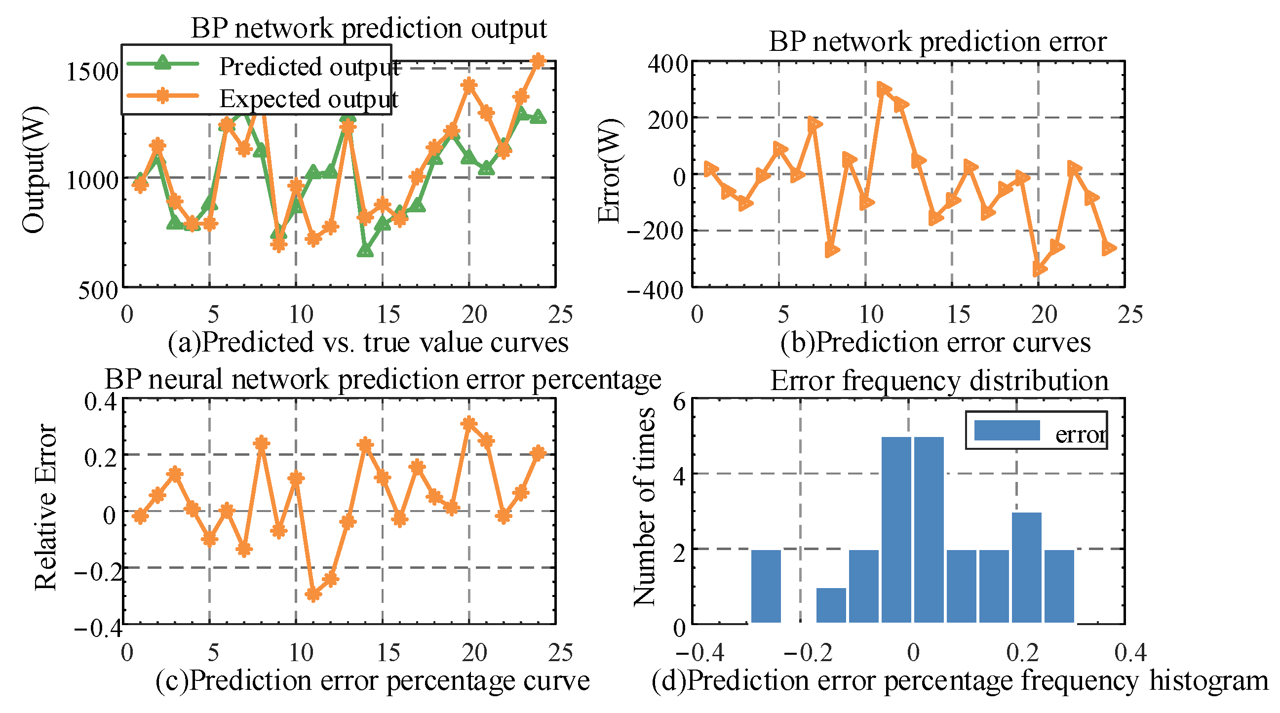
2. Renewable Energy and Load Forecast

Short-term forecasting of renewable energy and load in the system is an important part of rational day-ahead and intra-day dispatch [17]. (back propagation, BP) neural networks are typically characterized by their strong self-learning, adaptive and fault-tolerant capabilities in dealing with nonlinear probabilistic problems. As a result, BP neural networks can respond quickly and effectively to the environment and a range of stochastic factors, improving predictive power while achieving adaptivity through deeper learning and sampling training, hence the use of the method for renewable energy and load forecasting [16,17]. Figure 1. below shows the topology of the neural network. As shown in Figure 1, before predicting renewable energy and load, the topology of the BP neural network needs to be determined, and the number of implicit, input, and output layers in the structure used for this study is 1. The BP neural network uses the most rapid descent method as the default calculation method.

For features containing random fluctuation characteristics, such as load photovoltaic wind energy, the prediction of the traditional BP neural network is not stochastic and does not meet the stochastic characteristics of the above fluctuations because the weights and thresholds are obtained by initialization at the time of training. The genetic algorithm can effectively optimize the weights and thresholds to avoid falling into a local optimum, so a genetic algorithm improved BP neural network is used for renewable energy and load prediction, and the algorithm process is shown in Figure 2.

In short-term forecasting of renewable energy, as well as load based on BP neural network, the accuracy of forecasting, can be measured in terms of relative error as shown in the following equation.

$$e_{xd}=\frac{y_i-y_i^{\prime }}{y_i}\times 100\%$$

(1)

where $y_i$ denotes the true value and $y_i^{\prime }$ denotes the predicted value.

As shown in Figure 3, the BP neural network improved by the genetic algorithm can keep the relative error of each hour at less than 0.3% accuracy when predicting before the day, and after the statistical error frequency, the most concentration is 0.1%.

3. Scheduling Method of Source Network Load and Storage Coordination

The grid integration of renewable energy sources such as wind power and photovoltaic [3] brings many problems to the active distribution grid, such as causing drastic fluctuations in the system, increasing the net loss of the power system, and there are many renewable energy sources that cannot be consumed, it has become a challenge to mobilize the flexibility of source-grid-load-storage and deal with the economic problems of renewable energy consumption and distribution network operation [4,5,6,7].

Figure 4 shows the structure of an active distribution grid system with coordinated source-grid-load-storage interaction. It consists of four components, source, grid, load, and storage [12]. The optimization model focuses on the lowest cost of distribution grid operation and the lowest loss of actively managed devices.

The source side coordinates and complements the output timing and spatial distribution characteristics of controllable distributed renewable energy sources to reduce the impact of power fluctuations on the system and improve the consumption capacity [14]. The grid side rationally reconfigures the network structure of the active distribution network according to the network operation state [19]. Coordination of the temporal and spatial characteristics of the network resources. On the load side, the new power system contains many adjustable loads, such as air conditioning loads, which can cut peaks and fill valleys and relieve network congestion by guiding customers to change their electricity consumption patterns. In energy storage [13], due to the development of renewable energy electric vehicles, traditional energy storage devices and new mobile energy storage in the active distribution network can quickly adjust their charging and discharging power by the system’s dispatching commands, which can charge at low valley loads and discharge at peak loads, which helps to improve the system’s ability to cut peaks and fill valleys and improve the economy of operation.

3.1. Multi-Time Scale Scheduling Mode

A multi-timescale active distribution network coordination and optimal dispatching strategy are proposed for active distribution networks containing multiple flexible resource resources in the source-network-load-storage. The corresponding optimal control objectives are proposed from two-time scales: day-ahead and intra-day. In addition, correspondingly, the dispatching is divided into two stages: day-ahead optimization dispatching and intra-day optimization dispatching. In the day-ahead optimization stage, the grid company optimizes the dispatch according to the day-ahead market price, the flexible and controllable resources on the source-grid-load-storage side, etc., and determines the output of each piece of equipment, the amount of power purchased from the upper grid and the amount of flexible load regulation on the next day.

However, due to the relatively long prediction time scale, the gap between the prediction results of renewable energy and load and the actual situation becomes larger, resulting in a lack of practical guidance for the optimization results in the long-time scale, so further corrections are needed in the intra-day stage. On the basis of the scheduling with economic optimization as the control target, consider the coordination of each flexible resource in the short time scale within the day so as to achieve the maximum quality consumption of renewable energy. Correction of deviations between scheduling plan and forecast results. In summary, the architecture of the proposed multi-time-scale coordinated optimal scheduling method for active distribution networks is shown in Figure 5.

3.2. Scheduling Objective Function before the Day

In order to reasonably and effectively utilize the strong interactivity and dispatchability of multi-flexible resources, the dispatching costs of multi-flexible resources are integrated based on the consideration of distribution network operation costs, including wind abandonment costs, higher level power purchase costs, and network loss costs. In addition, the operating cost of (the capacitor, CB) and (On-Line Tap Changer, OLTC) is also introduced into the objective function of distribution network operation cost because the lifetime of CB and OLTC is affected by the number of operations.

$$\min F_{\mathrm{EC}}={\displaystyle \sum _{t=1}^T\left(\begin{array}{l}{C}_t^{abandon}+C_p^{buy}+C_t^{loss}\\ +C_t^{flex}+C_o^{CB}+C_o^{OLTC}\end{array}\right)}$$

(2)

where $C_t^{abandon}$ is the abandonment cost, $C_{p,t}^{buy}$ is the cost of active power purchase from the upper grid, $C_p^{buy}$ is the cost of power purchase from the distribution network, $C_t^{loss}$ is the cost of network losses, $C_t^{flex}$ is the cost of scheduling flexibility resources $C_o^{CB}$ and $C_o^{OLTC}$ are the operating costs of CB and OLTC.

$$C_t^{abandon}={\displaystyle \sum _{i\in {\Omega }_{\mathrm{DG}}}\left({\lambda }_{abandon}^{\mathrm{DG}}{P}_{i.t}^{\mathrm{DG}. abandon }\right)}\Delta t$$

(3)

where ${\lambda }_{abandon}^{\mathrm{DG}}$ is the cost per unit of distributed power supply, $P_{i.t}^{\mathrm{DG}. abandon }$ is the amount of power abandoned by the distributed power supply, $i$ is the node where the distributed power supply is located and ${\Omega }_{\mathrm{DG}}$ is the set of all points containing distributed power supply.

$$C_t^{buy}={\displaystyle \sum _{i={\Omega }_{\mathrm{DG}}}^{}{\lambda }_p^{buy.DG}{P}_{i,t}^{DG}\Delta t}+{\displaystyle \sum _{i={\Omega }_{grid}}^{}{\lambda }_p^{buy.grid}{P}_{i,t}^{grid}}\Delta t$$

(4)

where $C_t^{buy}$ is the cost of electricity purchased from the distribution network, ${\lambda }_p^{buy.DG}$${\lambda }_p^{buy.grid}$ is the renewable energy feed-in tariff and the electricity purchased from the distribution network, $P_{i,t}^{DG}$ and $P_{i,t}^{grid}$ are the electricity purchased from the distribution network to the renewable energy and the superior network.

$$C_t^{loss}={\lambda }^{loss}\left({\displaystyle \sum _{ij\in {\Omega }_{\mathit{SW}}}s}{w}_{ij.t}{I}_{ij.t}^2{R}_{ij}+{\displaystyle \sum _{ij\in {\Omega }_{\mathit{Close}}}{I}_{ij.t}^2}{R}_{ij}\right)\Delta t$$

(5)

where ${\lambda }^{loss}$ is the cost of network loss $s{w}_{ij.t}$ is the switching status of the branch $ij$, 0–1 variable, “0” means open, “1” means closed ${\Omega }_{SW}$ means the branch where the contact switch is located, ${\Omega }_{Close}$ means the branch where the normally closed switch is located.

$$C_t^{flex}=C_t^{DG}+C_t^{SVC}+C_t^{CB}+C_t^{SW}+C_t^{DR}+C_t^{ESS}$$

(6)

where the cost of scheduling flexible resources includes the cost of distributed power reactive power compensation $C_t^{DG}$, the cost of static reactive power generator compensation $C_t^{SVC}$, the cost of grouping capacitor compensation $C_t^{CB}$, the cost of dynamic reconfiguration of the distribution network $C_t^{SW}$, the cost of controlled load regulation $C_t^{DR}$, and the cost of energy storage and reactive power compensation $C_t^{ESS}$.

$$C_t^{DG}={\displaystyle \sum _{i\in {\Omega }_{\mathrm{DG}}}\left({\lambda }_q^{DG}\left|Q_{i.t}^{DG}\right|\right)}\Delta t$$

(7)

where ${\lambda }_q^{DG}$ is the unit reactive power compensation cost of distributed energy; ${\lambda }^{\mathrm{SW}}$ is the switching operation cost; ${\lambda }^{\mathit{DR}}$ is the unit regulation cost of the regulable load.

$$C_t^{SVC}={\displaystyle \sum _{i\in {\Omega }_{SVC}}\left({\lambda }_q^{SVC}\left|Q_{i.t}^{SVC}\right|\right)}\Delta t$$

(8)

where ${\lambda }_q^{SVC}$ is the stationary reactive power generator unit reactive power compensation cost bit regulation cost, $Q_{i.t}^{SVC}$ is the stationary reactive power generator compensation power, ${\Omega }_{SVC}$ is the set of nodes where the stationary reactive power generator is located.

$$C_t^{CB}={\displaystyle \sum _{i\in {\Omega }_{CB}}\left({\lambda }_q^{CB}\left|Q_{i.t}^{CB}\right|\right)}\Delta t$$

(9)

where ${\lambda }_q^{CB}$ is the cost per unit of reactive power compensation for the group-throwing capacitors, $Q_{i.t}^{CB}$ is the power of the group-throwing capacitors, and ${\Omega }_{CB}$ is the set of nodes where the static reactive power generators are located.

$$C_t^{SW}={\displaystyle \sum _{ij\in {\Omega }_{SW}}{\lambda }^{SW}}\Delta s{w}_{ij.t}$$

(10)

where ${\lambda }^{SW}$ is the unit action cost of the contact switch, $\Delta s{w}_{ij.t}$ is the number of times the contact switch is actuated and ${\Omega }_{SW}$ is the set of branch circuits where the contact switch is located.

$$C_t^{DR}={\displaystyle \sum _{i\in {\Omega }_{\mathrm{DR}}}\left({\lambda }^{DR}\left|P_{i.t}^{Load.a}-P_{i.t}^{Load.f}\right|\right)}\Delta t$$

(11)

where ${\lambda }^{DR}$ is the unit scheduling cost of controllable load, $P_{i.t}^{Load.a}$ and $P_{i.t}^{Load.f}$ are the load power and the original power of controllable load at node i after the time shift of flexibility, respectively. Ω_DR is the set of nodes accessed by controllable load respectively.

$$C_t^{ESS}={\displaystyle \sum _{i\in {\Omega }_{ESS}}{\lambda }_p^{ESS}}\left({\eta }_{i. \mathrm{cha} }^{ESS}{P}_{i.t.\mathrm{cha}}^{ESS}+\frac{P_{i.t \mathrm{discha} }^{ESS}}{{\eta }_{i. \mathrm{discha} }^{ESS}}\right)\Delta t+{\displaystyle \sum _{i\in {\Omega }_{ESS}}\left({\lambda }_q^{ESS}\left|Q_{i.t}^{ESS}\right|\right)}\Delta t$$

(12)

where ${\lambda }_p^{ESS}$ and ${\lambda }_q^{ESS}$ are the depreciation coefficients per unit of power for energy storage charging and discharging; ${\eta }_{i. \mathrm{cha} }^{ESS}$ indicates the energy storage charging efficiency; ${\eta }_{i. \mathrm{discha} }^{ESS}$ indicates the energy storage discharging efficiency; $P_{i.t. \mathrm{cha} }^{ESS}$ indicates the energy storage charging power; and $P_{i.t. \mathrm{discha} }^{ESS}$ indicates the energy storage discharging power.

$$C_o^{\mathrm{CB}}+C_o^{\mathrm{OLTC}}=c_o^{CB}{\displaystyle \sum _{t=1}^T{\displaystyle \sum _{i\in {\Omega }_{CB}}^l{\delta }_{i,t}^{CB}}}+c_o^{OLTC}{\displaystyle \sum _{t=1}^T\left({\delta }_{i,t}^{OLTC,IN}+{\delta }_{i,t}^{OLTC,DE}\right)}$$

(13)

3.3. Intraday Scheduling Objective Function

Short-term optimal dispatch model Different from the objective of day-ahead dispatch, the short-term dispatch takes the day-ahead dispatch result as the benchmark, adds constraints with the minimum operating cost of the distribution network, and achieves the maximum consumption of renewable energy through mutual cooperation and collaboration of energy storage, SVC and (Energy storage systems, ESS), and flexible load. The ultra-short-term forecasting of wind power and photovoltaic using a neural network is rolled over every 10 min, and the short-term dispatching plan is formulated on this basis.

The objective function of optimal short-term scheduling is shown as follows.

$$\max F_{DG}={\displaystyle \sum _{t=1}^{T_S}{\displaystyle \sum _{i\in {\Omega }_{DG}}{P}_{i.t}^{DG}}}\Delta t$$

(14)

where $F_{DG}$ is the renewable energy power consumption in the whole day of the distribution network, t is the time period identification (t = 1, 2, …, T), Δt is the time interval, T is the total number of time periods, this paper takes Δt = 1 h, T = 24, $P_{i.t}^{DG}$ is the actual renewable energy power consumption at node i, ${\Omega }_{DG}$ is the set of nodes corresponding to the scenery.

3.4. Constraints

3.4.1. Source Side Flexibility

Sources considered for source-side flexibility include OLTC as well as distributed energy sources.

On-load regulating transformers are able to change the output voltage by adjusting the position of the tap. Between the upper grid and the root node i of the distribution network, respectively.

$$\left\{\begin{array}{l}{V}_{i.\min }^2\le {\left(V_{i,t}^{\mathrm{Base} }\right)}^2{r}_{i,t}\le V_{i.\max }^2\hfill \\ r_i^{\min }\le r_{i,t}\le r_i^{\max }\hfill \end{array},\hspace{1em}\forall t,\forall i\in {\Omega }^{\mathrm{OLTC}}\right.$$

(15)

where ${\Omega }^{\mathrm{OLTC}}$ is the set of all substation nodes with on-load regulator transformers; $V_{i,t}^{\mathrm{Base} }$ is the voltage value on the high voltage side of the transformer, which is a constant value; $r_i^{\max }$ and $r_i^{\min }$ are the upper and lower limits of the OLTC ratio squared; $r_{i,t}$ is the OLTC ratio squared ratio, which can be described as the following relationship with 0–1 variables.

$$\left\{\begin{array}{l}{\sigma }_{i,1,t}^{OLTC}\ge {\sigma }_{i,2,t}^{OLTC}\ge {\sigma }_{i,{\mathrm{SR}}_i,t}^{OLTC},\forall t,\forall j\in {\Omega }^{OLTC};{\delta }_{i,t}^{OLTC,IN}+{\delta }_{i,t}^{OLTC,\mathrm{DE}}\le 1,\forall t,\forall j\in {\Omega }^{OLTC}\\ {\displaystyle \sum _s{\sigma }_{i,s,t}^{OLTC}}-{\displaystyle \sum _s{\sigma }_{i,s,t-1}^{OLTC}}\ge {\delta }_{i,t}^{OLTC,IN}-{\delta }_{i,t}^{OLTC,DE}{\mathrm{SR}}_j,\forall t,\forall i\in {\Omega }^{OLTC}\\ {\displaystyle \sum _s{\sigma }_{i,s,t}^{OLTC}}-{\displaystyle \sum _s{\sigma }_{i,s,t-1}^{OLTC}}\le {\delta }_{i,t}^{OLTC,IN}{\mathrm{SR}}_i-{\delta }_{i,t}^{OLTC,DE},\forall t,\forall j\in {\Omega }^{OLTC}\\ {\displaystyle \sum _{t\in T}\left({\delta }_{i,t}^{OLTC,IN}+{\delta }_{i,t}^{OLTC,DE}\right)}\le N_i^{OLTC,\max },\forall j\in {\Omega }^{OLTC}\end{array}\right.$$

(16)

where ${\delta }_{j,t}^{\mathit{OLTC},IN}$ and ${\delta }_{j,t}^{\mathit{OLTC},\mathit{DE}}$ are used to indicate OLTC gear adjustment; ${\mathrm{SR}}_j$ is the maximum range of OLTC gear change; $N_j^{\mathit{OLTC},\max }$ is the maximum number of OLTC gear adjustments allowed in T time period.

Controlled distributed energy sources need to consider their power factor limits and capacity limits, as well as climbing constraint limits, when participating in coordinated dispatch, as shown in the following equation.

$$\left\{\begin{array}{c}{P}_{i.t}^{DG}=P_{i.t}^{DG. \mathrm{av} }-P_{i.t}^{DG. \mathrm{abandon} }\\ -P_{i.t}^{DG}\tan \left({\cos }^{-1}P{F}_{i. \mathrm{down} }^{DG}\right)\le Q_{i.t}^{DG}\le \\ P_{i.t}^{DG}\tan \left({\cos }^{-1}P{F}_{i. \mathrm{up} }^{DG}\right)\\ {\left(P_{i.t}^{DG}\right)}^2+{\left(Q_{i.t}^{DG}\right)}^2\le {\left(S_i^{DG}\right)}^2\end{array}\right.$$

(17)

where $P_{i.t}^{DG}$ is the actual power output of distributed energy at $i$ node, $P_{i.t}^{DG. \mathrm{av} }$ is the active power output of distributed energy at $i$ node $P_{i.t}^{DG. \mathrm{abandon} }$ is the discarded power of distributed energy, $P{F}_{i. \mathrm{down} }^{DG}$ and $P{F}_{i. \mathrm{up} }^{DG}$ are the power factor values of distributed energy at $i$ node $S_i^{DG}$ is the capacity of distributed energy at $i$ node. $P_{i.t+1}^{DG}$ and $P_{i.t}^{DG}$ is the active power output of the distributed energy source at the next moment with the currently active power output.

$$\left.\left|P_{i.t+1}^{DG}-P_{i.t}^{DG}\right.\right|\le r_{\lim ,i}$$

(18)

where $P_{i.t+1}^{\mathrm{DG} }$ and $P_{i.t}^{\mathrm{DG} }$ are the active output of the distributed energy source at the next moment and the currently active output, and $r_{\lim ,i}$ is the up and down slope limit value.

3.4.2. Network Side Flexibility

Active distribution network reconfiguration requires frequent opening and closing of contact switches, reducing switch life.

Therefore, it is necessary to limit the number of switch actions in dynamic reconfiguration as follows.

$$\Delta s{w}_{ij.t}=\left|s{w}_{ij.t}-s{w}_{ij.t-1}\right|$$

(19)

$${\displaystyle \sum _{t=1}^T\Delta }s{w}_{ij.t}⩽s{w}_{ij.\max }^{\mathrm{unit}}$$

(20)

where $s{w}_{ij.\max }^{\mathrm{unit}}$ is the maximum allowable number of operations of the branch ij throughout the day.

$$\left\{\begin{array}{l}{\displaystyle \sum _{ij\in {\Omega }_{SW}}s}{w}_{ij.t}+N_{\mathrm{Close} }=N-N_{\mathrm{S}}\hfill \\ {\displaystyle \sum _{ij\in {\Omega }_{SW.l}}s}{w}_{ij.t}+N_{\mathrm{Close} .l}⩽M_l-1\hfill \end{array}\right.$$

(21)

where $N$, $N_{\mathrm{S}}$ and $N_{\mathrm{Close} }$ are the total number of nodes, the number of root nodes, and the total number of normally closed branches in the network, respectively, $M_l$ is the number of branches in the lth power supply loop, l = 1, 2, …, L, L is the total number of power supply loops in the network, $s{w}_{ij.t}$ is the remote switch state of branch ij in the lth power supply loop, ${\Omega }_{SW.l}$ and $N_{\mathrm{Close} .l}$ are the set of branches with remote switches in the lth power supply loop respectively.

3.4.3. Load Side Flexibility

The capacitor bank operation model can be expressed as:

$$\left\{\begin{array}{l}{Q}_{i,t}^{CB}=y_{i,t}^{CB}{Q}_i^{CB, \mathrm{step} }\hfill \\ y_{i,t}^{CB}\le Y_i^{CB,\max }\hfill \end{array},\hspace{1em}\forall t,\forall j\in {\Omega }^{CB}\right.$$

(22)

where $Q_j^{CB, \mathrm{step} }$ is the compensation amount of group-throwing capacitors per slot; ${\Omega }^{\mathit{CB}}$ is the set of nodes; $Y_j^{CB,\max }$ is the upper limit of the number of throwing groups; $y_{j,t}^{CB}$ is the number of throwing groups. When considering the economics and lifetime of the equipment, the capacitors are subject to a regulation constraint, so the total number of operations for multiple periods is considered.

$${\displaystyle \sum _{t\in T}\left|y_{j,t}^{CB}-y_{j,t-1}^{CB}\right|}\le N_j^{CB,\max },\hspace{1em}\forall t,\forall j\in {\Omega }^{CB}$$

(23)

where $N_j^{CB,\max }$ is the maximum number of operable operations.

$$Q_i^{SVC,\min }\le Q_{i,t}^{SVC}\le Q_i^{SVC,\max },\hspace{1em}\forall t,\forall i\in {\Omega }^{SVC}$$

(24)

where is the section $B^{\mathit{SVC}}$ points $Q_j^{\mathit{SVC},\min }$ set, $Q_j^{\mathit{SVC},\max }$ are the upper and lower limits of the SVC output force respectively.

Distribution network loads such as central air conditioning and electric vehicles have certain controllability and flexibility, which can realize the spatial and temporal transfer of electricity consumption loads under certain rules and have a good ability to cut peaks and fill valleys and optimize load distribution. Equation (23) indicates the limitation of the controllable load’s own regulation capacity in the process of participating in the cooperative scheduling of multi-flexible resources, and Equation (24) indicates that the total electricity consumption of controllable load in a day is consistent with that before regulation.

$$\left\{\begin{array}{l}\begin{array}{l}{P}_{i,t}^{Load.a}=P_{i,t}^{Load.f}{k}_{i,t}^{}\\ Q_{i,t}^{Load.a}=Q_{i,t}^{Load.f}{k}_{i,t}^{}\end{array}\hfill \\ \left(1-k_i^{}\right)\le k_{i.t}^{}\le \left(1+k_i^{}\right)\hfill \end{array}\right.$$

(25)

$$\left\{\begin{array}{l}{\displaystyle \sum _{t=1}^T{P}_{i,t}^{Load.a}}\Delta t={\displaystyle \sum _{t=1}^T{P}_{i,t}^{Load.f}}\Delta t\hfill \\ {\displaystyle \sum _{t=1}^T{Q}_{i,t}^{Load.a}}\Delta t={\displaystyle \sum _{t=1}^T{Q}_{i,t}^{Load.f}}\Delta t\hfill \end{array}\right.$$

(26)

where $P_{i,t}^{Load.a}$ $Q_{i,t}^{Load.a}$ represents the flexible load-adjusted power output and $P_{i,t}^{Load.f}$ $Q_{i,t}^{Load.f}$ represents the original system load. $k_{i.t}^{}$ indicates the limit value of the controllable load variation time shift rate. In the incentive-based demand response model, the load variation time shift rate can usually be set by the grid scheduler on the day before the demand response, and the controllable load is dispatched on the response day.

3.4.4. Storage Side Flexibility

In general, energy storage flexibility modeling needs to consider constraints for multiple time periods. In order to extend the life of energy storage and prevent overcharging and discharging, it needs to consider its own capacity constraints, charging and discharging state constraints, and charging and discharging power constraints.

$$\left\{\begin{array}{l}{E}_{i,t+1}^{}=E_{i,t}+{\eta }_{i. \mathrm{cha} }^{ESS}{P}_{i.t. \mathrm{cha} }^{ESS}-{\eta }_{i. \mathrm{discha} }^{ESS}{P}_{i.t. \mathrm{discha} }^{ESS}\\ E_i^{\min }\le E_{i,t}\le E_i^{\max }, E_{i,t=0}=E_{i.t=T}\end{array}\right.$$

(27)

where $E_{i,t}$ indicates the current moment of energy storage and $E_{i,t+1}^{}$ indicates the next moment of energy storage.

$${\delta }_{i,.\mathrm{cha} }^{ESS}+{\delta }_{i.t \mathrm{discha} }^{ESS}\le 1$$

(28)

where ${\delta }_{i,.\mathrm{cha} }^{ESS}$, ${\delta }_{i.t \mathrm{discha} }^{ESS}$ indicates the charging and discharging state of energy storage, which cannot be in charging and discharging state at the same time.

$$\left\{\begin{array}{l}{\delta }_{i,.\mathrm{cha} }^{ESS}{P}_{i.t \mathrm{cha},\min }^{ESS}\le P_{i.t \mathrm{cha} }^{ESS}\le {\delta }_{i,.\mathrm{cha} }^{ESS}{P}_{i.t \mathrm{cha},\max }^{ESS}\hfill \\ {\delta }_{i,.\mathrm{discha} }^{ESS}{P}_{i.t \mathrm{discha},\min }^{ESS}\le P_{i.t \mathrm{discha} }^{ESS}\le {\delta }_{i,.\mathrm{discha} }^{ESS}{P}_{i.t \mathrm{cha},\max }^{ESS}\hfill \end{array}\right.$$

(29)

3.4.5. Distribution Grid Side Constraints

The distribution network tidal constraint is based on the Distflow branch tidal model, as Equations are shown.

$${\displaystyle \sum _{i\in u(j)}\left(P_{ij,t}-\frac{P_{ij,t}^2+Q_{ij,t}^2}{U_{i,t}^2}{r}_{ij}\right)}=P_{j,t}+{\displaystyle \sum _{k\in t(j)}{P}_{jk,t}}$$

(30)

$${\displaystyle \sum _{i\in u(j)}\left(Q_{ij,t}-\frac{P_{ij,t}^2+Q_{ij,t}^2}{U_{i,t}^2}{x}_{ij}\right)}=Q_{j,t}+{\displaystyle \sum _{k\in t(j)}{Q}_{jk,t}}$$

(31)

$$U_{i,t}^2-U_{j,t}^2=2\left(r_{ij}{P}_{ij,t}+x_{ij}{Q}_{ij,t}\right)-I_{ij,t}^2\left(r_{ij}^2+x_{ij}^2\right)$$

(32)

$$P_{i,t}^{grid}=P_{i,t}^{Load.a}-P_{i,t}^{DG}-P_{i,t.discha}^{ESS}+P_{i,t.cha}^{ESS}+{\displaystyle \sum _{j\in {\Omega }_{Close.i}}{P}_{ij.t}}+{\displaystyle \sum _{j\in {\Omega }_{SW.I}}{P}_{ij.t}s{w}_{ij.t}}$$

(33)

$$Q_{{}_{i,t}}^{grid}=Q_{i,t}^{\mathrm{Load}}-Q_{i,t}^{DG}-Q_{i,t}^{\mathrm{SVC}}-Q_{i,t}^{\mathrm{CB}}+{\displaystyle \sum _{j\in {\Omega }_{Close.i}}{Q}_{ij.t}}+{\displaystyle \sum _{j\in {\Omega }_{SW.I}}{Q}_{ij.t}s{w}_{ij.t}}$$

(34)

where $u(j)$ is the set of first nodes in the distribution network with j as the last node; $t(j)$ is the set of last nodes in the distribution network with j as the first node; $P_{i,t}^{grid}$ and $Q_{{}_{i,t}}^{grid}$ are the purchasing power from the superior grid $r_{ij}$ and $x_{ij}$ are the resistance and reactance of branch ij; $I_{ij,t}$ is the transmission current of branch ij; $U_{i,t}$ is the node voltage magnitude.

Equations (30)–(32) are non-convex constraints, which are relaxed and transformed into linear constraints using second-order cone-convex optimization techniques, and quickly find the optimal global solution; define the new variables node voltage value squared ${\tilde{U}}_{i,t}$ and branch current value squared ${\tilde{I}}_{ij,t}$.

$${\tilde{U}}_{i,t}=U_{i,t}^2$$

(35)

$${\tilde{I}}_{ij,t}⩾\frac{P_{ij,t}^2+Q_{ij,t}^2}{{\tilde{U}}_{i,t}}$$

(36)

After an equivalent deformation, transformed into the standard second-order cone form.

$${‖\begin{array}{c}2P_{ij,t}\\ 2Q_{ij,t}\\ {\tilde{I}}_{ij,t}-{\tilde{U}}_{i,t}\end{array}‖}_2⩽{\tilde{I}}_{ij,t}+{\tilde{U}}_{i,t}$$

(37)

Therefore, the branch tidal constraint can be deformed as

$$\left\{\begin{array}{l}{\displaystyle \sum _{i\in u(j)}\left(P_{ij,t}-{\tilde{I}}_{ij,t}{r}_{ij}\right)}=P_{j,t}+{\displaystyle \sum _{k\in v(j)}{P}_{jk,t}}\hfill \\ {\displaystyle \sum _{i\in u(j)}\left(Q_{ij,t}-{\tilde{I}}_{ij,t}{x}_{ij}\right)}=Q_{j,t}+{\displaystyle \sum _{k\in t(j)}{Q}_{jk,t}}\hfill \\ {\tilde{U}}_{i,t}-{\tilde{U}}_{j,t}=2\left(r_{ij}{P}_{ij,t}+x_{ij}{Q}_{ij,t}\right)-{\tilde{I}}_{ij,t}\left(r_{ij}^2+x_{ij}^2\right)\hfill \\ {‖\begin{array}{c}2P_{ij,t}\\ 2Q_{ij,t}\\ {\tilde{I}}_{ij,t}-{\tilde{U}}_{i,t}\end{array}‖}_2⩽{\tilde{I}}_{ij,t}+{\tilde{U}}_{i,t}\hfill \end{array}\right.$$

(38)

The voltage and current safety limits of the distribution network are shown below.

$$U_{i,\min }^2 ⩽{\tilde{U}}_{i,t}⩽U_{i,\max }^2$$

(39)

$$I_{ij,\min }^2 ⩽{\tilde{I}}_{ij,t}⩽I_{ij,\max }^2$$

(40)

where $U_{i,\min }^{}$ and $U_{i,\max }^{}$ are the upper and lower branch voltage limits for node i, and $I_{ij,\min }^{}$ and $I_{ij,\max }^{}$ are the upper and lower branch ij current limits.

Interaction power constraints.

$$\left\{\begin{array}{l}-P_{i. \mathrm{up} }^{\mathrm{grid} }⩽P_{i.t}^{\mathrm{grid} }⩽P_{i. \mathrm{up} }^{\mathrm{grid} }\hfill \\ -Q_{i. \mathrm{up} }^{\mathrm{grid} }⩽Q_{i.t}^{\mathrm{grid} }⩽Q_{i. \mathrm{up} }^{\mathrm{grid} }\hfill \end{array}\right.$$

(41)

where $P_{i. \mathrm{up} }^{\mathrm{grid} }$ and $Q_{i. \mathrm{up} }^{\mathrm{grid} }$ are the active and reactive power limits for the interaction between the upper grid and the root node i of the distribution network, respectively.

3.5. Linearization Strategy

The linearization approach used includes techniques such as variable substitution, segmented linearization, and the Big M method to linearize the nonlinear terms in the text, in turn, with the following process.

Equations (7)–(9) and (12) are linearized in the same way, and Equation (7) is used as an example for illustration.

Equation (7) is an absolute value function, so it needs to be linearized and introduces auxiliary variables with 0–1 variables, combined with the large M method equivalently linearized as:

$$\left\{\begin{array}{l}{C}_t^{DG}={\displaystyle \sum _{i\in {\Omega }_{\mathrm{DG}}}\left({\lambda }_q^{DG}{Q}_{i.t}^{\mathrm{av}}\right)}\Delta t\\ 0\le Q_{i.t}^{\mathrm{av}}-Q_{i.t}^{\mathrm{DG}}\le M_{DG,t}{\sigma }_{i,t}^{DG,1}\\ 0\le Q_{i.t}^{\mathrm{av}}-Q_{i.t}^{\mathrm{DG}}\le M_{DG,t}{\sigma }_{i,t}^{DG,2}\\ {\sigma }_{i,t}^{DG,1}\cdot {\sigma }_{i,t}^{DG,2}=0\end{array}\right.$$

(42)

where $Q_{i.t}^{\mathrm{av}}$ is the auxiliary variable, $M_{DG,t}$ is a large enough positive number, ${\sigma }_{i,t}^{DG,1}$ and ${\sigma }_{i,t}^{DG,2}$ is a 0–1 variable.

Equations (11), (18), (19), and (23) are linearized in the same way, and Equation (11) is used as an example to illustrate.

$$\left\{\begin{array}{l}{C}_t^{\mathrm{DR}}={\displaystyle \sum _{i\in {\Omega }_{\mathrm{DR}}}\left({\lambda }^{\mathrm{DR}}{P}_{i.t}^{\mathrm{Load}.\mathrm{av} }\right)}\Delta t\hfill \\ 0⩽P_{i.t}^{\mathrm{Load}.\mathrm{av} }-\left(P_{i.t}^{\mathrm{Load}. \mathrm{a}}-P_{i.t}^{\mathrm{Load}.\mathrm{f} }\right)⩽M_{\mathrm{Load}.t}{\sigma }_{i.t}^{\mathrm{Load}.1}\hfill \\ 0⩽P_{i.t}^{\mathrm{Load}.\mathrm{av} }+\left(P_{i.t}^{\mathrm{Load}.\mathrm{a}}-P_{i.t}^{\mathrm{Load}.\mathrm{f} }\right)⩽M_{\mathrm{Load}.t}{\sigma }_{i.t}^{\mathrm{Load}.2}\hfill \\ {\sigma }_{i.t}^{\mathrm{Load}.1}\cdot {\sigma }_{i.t}^{\mathrm{Load}.2}=0\hfill \end{array}\right.$$

(43)

where $P_{i.t}^{\mathrm{Load}.\mathrm{av} }$ is the auxiliary variable; $M_{\mathrm{Load}.t}$ and $M_{\mathrm{Load}.t}$ is a sufficiently large positive number in the large M method. ${\sigma }_{i.t}^{\mathrm{Load}.1}$ and ${\sigma }_{i.t}^{\mathrm{Load}.2}$ are 0–1 variables.

The nonlinear characteristics of the capacity constraint in Equation (17) due to the squared term are linearized using a segmental linearization.

$$\left\{\begin{array}{l}{\rho }_{i,t}^{\mathrm{DG},n}=a_i^{\mathrm{DG}\cdot n}{P}_{i,t}^{\mathrm{DG}}+b_i^{\mathrm{DG}.n}{Q}_{i.t}^{\mathrm{DG}}+c_i^{\mathrm{DG}.n}\hfill \\ {\rho }_{i,t}^{\mathrm{DG},n}⩾0\hspace{1em}{c}_i^{\mathrm{DG}.n}⩾0\hspace{1em}n=1,\cdots ,N^{\mathrm{DG}}\hfill \end{array}\right.$$

(44)

where n is the linearized segment number, $a_i^{\mathrm{DG}\cdot n}$ $b_i^{\mathrm{DG}.n}$ $c_i^{\mathrm{DG}.n}$ is the coefficient of the Nth line segment, and NDG is the number of linearized segments with capacity constraint.

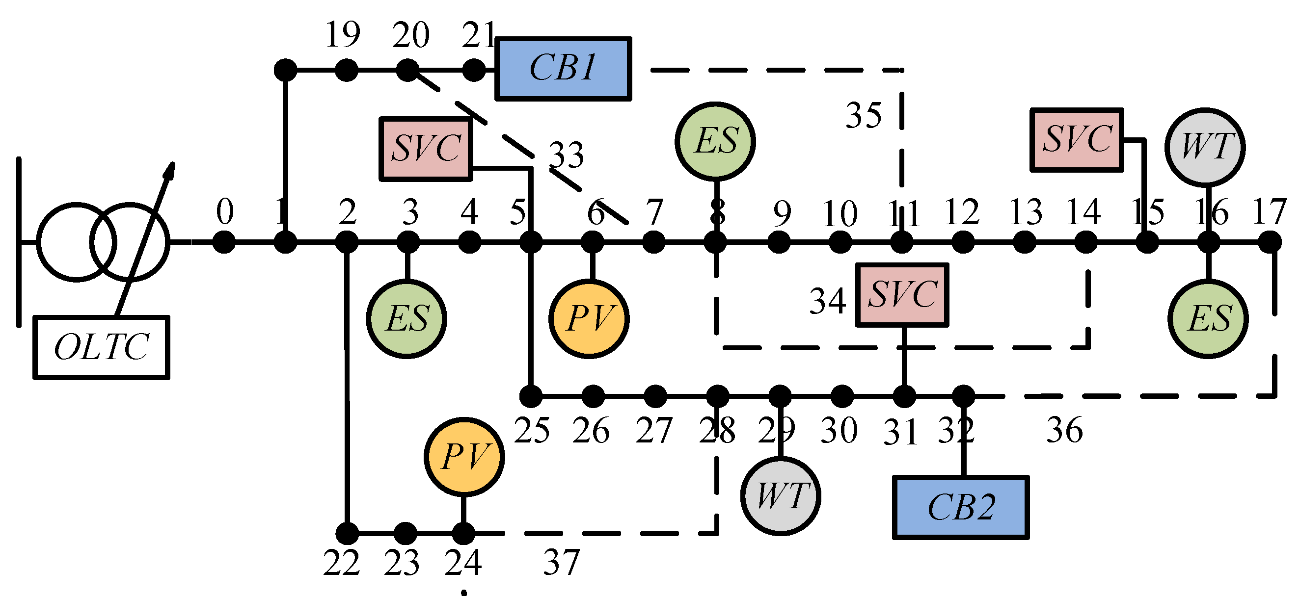
4. Example Validation

The IEEE 33-node distribution system shown in Figure 6. is used for simulation testing, where the voltage reference value is 12.66 kV, and the capacity reference value is 10 MVA. CB is connected to nodes 21 and 32, ES is connected to nodes 3, 8, and 16, PV is connected to nodes 6 and 24, WT is connected to nodes 16 and 29, and the access capacity is shown in the

Table 1. Renewable energy configurations.

Access Nodes	6	16	24	29
Access to renewable energy types	PV	WT	PV	WT
Access capacity/kW	1000	1600	1000	1600

. below.

The validity of the method is verified based on the following three methods.

(1) The optimal scheduling strategy of a multi-time scale distribution network with coordinated interaction of source network, load, and storage is proposed.

(2) Optimal scheduling on a single time scale.

(3) Not considering the dynamic reconfiguration of the distribution network and renewable energy consumption.

The following Table 1,

Table 2. ESS parameters.

Access Nodes	Power Limit/MW	Capacity Limit (MW-h)	Charging Efficiency	Discharge Efficiency
3	0.3	1.8	0.9	1.11
8	0.2	1	0.9	1.11
16	0.2	1.5	0.9	1.11

,

Table 3. CB parameters.

Access Nodes	Unit Capacity/Kvar	Quantity
21, 32	100	2

,

Table 4. SVC parameters.

Access Nodes	Compensation Range/Kvar
5, 15, 31	[−100, 300]

and

Table 5. OLTC parameters.

Parameters	Node Voltage/p.u.	OLTC Secondary Voltage/p.u.
Lower limit	0.93	0.95
Upper limit	1.07	1.05

show the configurations of renewable energy storage, on-load regulation transformers (OLTC), a grouping of capacitor banks (CB), and static VAR compensation for the IEEE 33-node system.

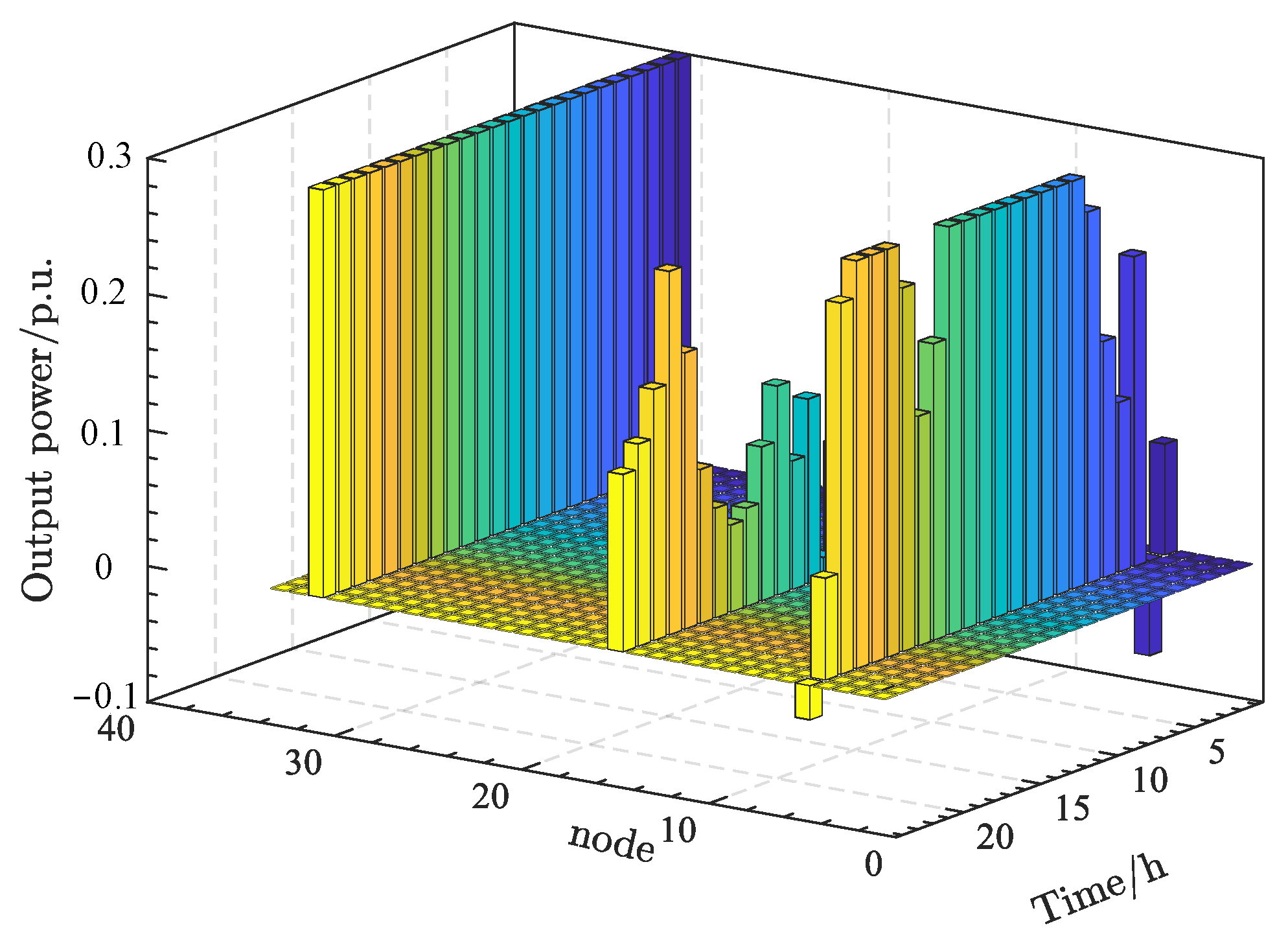
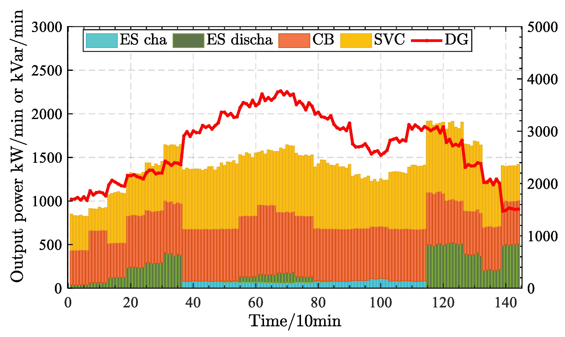
Analysis of Simulation Results

For the 33-node distribution network system, the above three methods are used to dispatch the distribution network. Among them, the renewable energy consumption and operation cost of the distribution network is shown in the following table, and the abandoned power and voltage of each time period are shown in the figure.

From the

Table 6. Operating cost and consumption rate.

Programs	FEC/104 CNY	Consumption Rate
1	2.083	93.87
2	2.39	88.52
3	2.8251	76.36

and Figure 7, it can be seen that the renewable energy consumption rate and consumption rate, as well as the operation cost of the distribution network obtained by this method, are the best. Compared with method 2 and method 3, the renewable energy consumption rate increased by 5.35% and 24.39%, respectively, and the operation cost is reduced by 7.96% and 18.28%, respectively.

The

Table 7. The economic cost of the three methods.

Programs	Cost of Abandoned Electricity/104 CNY	Flexibility and Operating Costs/104 CNY	Net Loss Cost/104 CNY	Cost of Electricity Purchase/104 CNY
1	0.356	0.075	0.555	1.585
2	0.512	0.112	0.402	1.698
3	1.025	0.289	0.511	1.432

. below shows that the abandonment cost of this method decreases by 0.156 × 10⁴ CNY and 0.669 × 10⁴ CNY compared to Option 2 and Option 3, respectively. Although this method incorporates various flexibility control measures, the flexible interaction cost is still reduced by 0.214 × 10⁴ CNY compared with method 3. This is due to the fact that the proposed model takes into account the requirements of power consumption and operation economy, so it can reasonably utilize the flexible interaction characteristics of multiple flexible resources to maximize the consumption of renewable energy with minimum operation cost, while Method 3 ignores the spatial and temporal complementarity between the active management components due to the flexibility of the distribution network structure. The network loss cost and power purchase cost of this method is higher than those of methods 2 and 3 because the flexible interaction of multi-flexible resources is used to promote renewable energy consumption, which leads to reverse power transmission and increases the line loss, thus increasing the network loss and the power and power purchase cost of renewable energy.

For the IEEE33 node system, the distribution network dispatch based on the strategy is shown in Figure 8, Figure 9, Figure 10, Figure 11, Figure 12, Figure 13 and Figure 14 below.

Figure 8 and Figure 9 show the voltage distribution and branch current carrying capacity before and after dispatching, respectively. It can be seen that before dispatching, due to the access to renewable energy sources and the lack of system flexibility regulation ability, the distribution network had an over-voltage limit and excessive voltage fluctuation, compared with after implementing the dispatching strategy, the node voltage of the distribution network obviously relieves the phenomenon of excessive voltage deviation and over-voltage limit, and the system carrying capacity also decreases significantly. Figure 10 shows the ES output, Figure 11 shows the CB output, Figure 12 shows the SVC output, and Figure 13 and Figure 14 show the day-ahead and intra-day dispatching, respectively. The comprehensive experimental results above show that the performance of all aspects of the scheme system has been effectively improved before and after the source-grid-load-storage interaction. From the above figure, it can be seen that the proposed method has a good effect in alleviating the under-voltage and smoothing the voltage fluctuation of the power system. The following

Table 8. Reconstruction results.

Whether to Reconfigure	Number of Reconfigurations	Reconfiguration Moment	Disconnect Switch Number	Total Network Loss/kW·h
Yes	4	0:00	7/11/14/17/28	1925.13
		4:00	7/9/14/28/32
		19:00	7/9/14/28/36
		21:00	7/9/14/17/37
No	0		33/34/35/36/37	2258.72

. and Figure 15. show the topology of the distribution system for each time period

From the distribution network structure and net loss in Figure 15, it can be seen that the total network loss of the distribution network in a day is reduced by 466.41 kwh before and after reconfiguration, and it maintains a radial operation. The distribution network reconfiguration is equivalent to changing the topology to transfer the load to another branch with a lower load level at a certain load peak and to transfer the renewable energy to the rest of the branch when the renewable energy output is high, and it is difficult to be consumed by this branch to achieve the purpose of space-time coordination.

5. Conclusions

In order to explore the synergy capability of source-grid load and storage in the AC distribution network, a multi-timescale optimal dispatch model considering the operating cost of the distribution network and renewable energy consumption is developed. The method considers the synergistic capability of source-grid load and energy storage in the system and achieves good results based on the multi-timescale idea and second-order cone relaxation technique. The flexible resources in the distribution network are modeled interactively in a comprehensive manner to give full play to the complementarity of resources and significantly improve renewable energy consumption and grid operation costs. The following three points summarize the contributions of the study.

(1) The mathematical model of each component in the distribution network is carefully established on the basis of an in-depth study of the coordination of the flexible resources on the source grid, load-storage side to promote the economic operation of the distribution network, and the high-quality consumption of renewable energy. The experimental results show that the economy of the system has improved by 18.28% compared with that before optimization, and the system’s consumption rate of renewable energy has increased by 24.39%.

(2) The optimal dispatching strategy for the coordinated operation of the source network, load, and storage is diverse, and the integrated day-ahead and day-ahead dispatching model is more consistent with the actual situation, which can economically and effectively coordinate the resources on the source network, load, and storage side to achieve the purpose of minimizing the operation cost of the distribution network and optimizing the consumption of renewable energy.

(3) The solution idea of the second-order cone optimal tide framework is chosen and based on the linearized model, which can ensure the optimal solution result while significantly reducing the solution difficulty and improving the solution efficiency.

Finally, how to consider the collaborative dispatching between multiple types of energy in active distribution networks and the study of artificial intelligence-based distribution network dispatching are directions that we can continue to study in the future.

References

1. Javaid, N.; Hafeez, G.; Iqbal, S.; Alrajeh, N.; Alabed, M.S.; Guizani, M. Energy efficient integration of renewable energy sources in the smart grid for demand side management. IEEE Access 2018, 6, 77077–77096. [Google Scholar] [CrossRef]
2. AHadi, A.; Silva, C.A.S.; Hossain, E.; Challoo, R. Algorithm for demand response to maximize the penetration of renewable energy. IEEE Access 2020, 8, 55279–55288. [Google Scholar]
3. Guo, Y.; Wu, Q.; Gao, H.; Chen, X.; Østergaard, J.; Xin, H. MPC-based coordinated voltage regulation for distribution networks with distributed generation and energy storage system. IEEE Trans. Sustain. Energy 2019, 10, 1731–1739. [Google Scholar] [CrossRef] [Green Version]
4. Joo, J.-Y.; Raghavan, S.; Sun, Z. Integration of sustainable manufacturing systems into smart grids with high penetration of renewable energy resources. In Proceedings of the 2016 IEEE Green Technologies Conference (GreenTech), Kansas City, MO, USA, 6–8 April 2016; pp. 12–17. [Google Scholar]
5. Dorostkar-Ghamsari, M.R.; Fotuhi-Firuzabad, M.; Lehtonen, M.; Safdarian, A. Value of distribution network reconfiguration in presence of renewable energy resources. IEEE Trans. Power Syst. 2016, 31, 1879–1888. [Google Scholar] [CrossRef]
6. Gao, P.; Chen, H.; Zheng, X.; Wu, B. Framework planning of active distribution network considering active management. J. Eng. 2017, 2017, 2093–2097. [Google Scholar] [CrossRef]
7. Zhang, C.; Lin, Z.; Wen, F.; Ledwich, G.; Xue, Y. Two-stage power network reconfiguration strategy considering node importance and restored generation capacity. IET Generat. Transmiss. Distrib. 2014, 8, 91–103. [Google Scholar] [CrossRef]
8. Petrichenko, L.; Varfolomejeva, R.; Gavrilovs, A.; Sauhats, A.; Petricenko, R. Evaluation of battery energy storage systems in distribution grid. In Proceedings of the 2018 IEEE International Conference on Environment and Electrical Engineering and 2018 IEEE Industrial and Commercial Power Systems Europe (EEEIC/I&CPS Europe), Palermo, Italy, 12–15 June 2018; pp. 1–6. [Google Scholar]
9. Gao, H.; Wang, L.; Liu, J.; Wei, Z. Integrated Day-Ahead Scheduling Considering Active Management in Future Smart Distribution System. IEEE Trans. Power Syst. 2018, 33, 6049–6061. [Google Scholar] [CrossRef]
10. Atteya, I.I.; Ashour, H.; Fahmi, N.; Strickland, D. Radial distribution network reconfiguration for power losses reduction using a modified particle swarm optimization. CIRED-Open Access Proc. J. 2017, 2017, 2505–2508. [Google Scholar] [CrossRef] [Green Version]
11. Baharvandi, A.; Aghaei, J.; Nikoobakht, A.; Niknam, T.; Vahidinasab, V.; Giaouris, D.; Taylor, P. Linearized Hybrid Stochastic/Robust Scheduling of Active Distribution Networks Encompassing PVs. IEEE Trans. Smart Grid 2020, 11, 357–367. [Google Scholar] [CrossRef]
12. Zhang, Y.; Ji, Y.; Wu, M.; Ding, B.; Yu, H.; Kou, L. Optimal dispatching of regional integrated energy system based on SMPC. In Proceedings of the 2020 IEEE 4th Conference on Energy Internet and Energy System Integration (EI2), Wuhan, China, 30 October–1 November 2020; pp. 4092–4096. [Google Scholar]
13. Chen, Q.; Zhao, X.; Gan, D. Active-reactive scheduling of active distribution system considering interactive load and battery storage. Protect. Control Mod. Power Syst. 2017, 2, 320–330. [Google Scholar] [CrossRef] [Green Version]
14. Gao, H.; Liu, J.; Wang, L. Robust coordinated optimization of active and reactive power in active distribution systems. IEEE Trans. Smart Grid 2018, 9, 4436–4447. [Google Scholar] [CrossRef]
15. Li, X.; Han, X.; Yang, M. Day-Ahead Optimal Dispatch Strategy for Active Distribution Network Based on Improved Deep Reinforcement Learning. IEEE Access 2022, 10, 9357–9370. [Google Scholar] [CrossRef]
16. Han, A.; Zhou, S.; Jian, X.; Li, Z. Safe and Economic Dispatching Model of Distribution Network Based on Cloud Particle Swarm Optimization Algorithm. In Proceedings of the 2022 7th International Conference on Intelligent Computing and Signal Processing (ICSP), Xi’an, China, 15–17 April 2022; pp. 900–903. [Google Scholar]
17. Li, Y.; Fan, X.; Cai, Z.; Yu, B. Optimal active power dispatching of microgrid and distribution network based on model predictive control. Tsinghua Sci. Technol. 2018, 23, 266–276. [Google Scholar] [CrossRef] [Green Version]
18. Zhang, T.; Li, X.; Yu, H.; Liu, J.; Zeng, P.; Sun, L. A Fault Location Method for Active Distribution Network with Renewable Sources Based on BP Neural Network. In Proceedings of the 2015 7th International Conference on Intelligent Human-Machine Systems and Cybernetics, Hangzhou, China, 26–27 August 2015; pp. 357–361. [Google Scholar] [CrossRef]
19. Ning, L.; Guo, Z.; Chen, C.; Zhou, E.; Zhang, L.; Wang, L. Short-term Forecasting Model of Regional Power Load Based on Neural Network. In Proceedings of the 2019 IEEE 7th International Conference on Computer Science and Network Technology (ICCSNT), Dalian, China, 19–20 October 2019; pp. 241–245. [Google Scholar] [CrossRef]
20. Guo, W.; Yu, L.; Han, A.; Li, Z. Optimal Dispatch Model of Active Distribution Network Based on Particle Swarm optimization Algorithm with Random Weight. In Proceedings of the 2021 IEEE 2nd International Conference on Big Data, Artificial Intelligence and Internet of Things Engineering (ICBAIE), Nanchang, China, 26–28 March 2021; pp. 482–485. [Google Scholar] [CrossRef]
21. Saini, P.; Gidwani, L. Optimum utilization of photovoltaic generation with battery storage in distribution system by utilizing genetic algorithm. In Proceedings of the 2020 IEEE International Conference on Power Electronics, Drives and Energy Systems (PEDES), Jaipur, India, 16–19 December 2020; pp. 1–6. [Google Scholar] [CrossRef]
22. Sheng, H.; Wang, C.; Liang, J. Multi-timescale active distribution network optimal scheduling considering temporal-spatial reserve coordination. Int. J. Elect. Power Energy Syst. 2021, 125, 106526. [Google Scholar] [CrossRef]
23. Luo, F.; Jiao, Z.; Yao, L.; Zhu, L.; Zhao, D.; Qian, M. Second-order Cone Relaxation based Optimization Method of Optimal Operation of Distribution Systems with Integrated Energy. In Proceedings of the 2021 3rd Asia Energy and Electrical Engineering Symposium (AEEES), Chengdu, China, 26–29 March 2021; pp. 1150–1154. [Google Scholar] [CrossRef]
Figure 1. BP neural network topology diagram.
Energies 16 01356 g001
Figure 2. Flow chart of BP neural network improved by genetic algorithm.
Energies 16 01356 g002
Figure 3. The predictive power of the BP neural network was improved by the genetic algorithm Figure.
Energies 16 01356 g003
Figure 4. Schematic diagram of the optimal scheduling model based on the coordinated interaction of source, network, load, and storage.
Energies 16 01356 g004
Figure 5. Multi-timescale optimization schematic.
Energies 16 01356 g005
Figure 6. IEEE 33-node distribution network.
Energies 16 01356 g006
Figure 7. Abandoned electricity.
Energies 16 01356 g007
Figure 8. System node voltage and current before scheduling.
Energies 16 01356 g008
Figure 9. System node voltage and current after scheduling.
Energies 16 01356 g009
Figure 10. ESS Spatial and temporal distribution of power output.
Energies 16 01356 g010
Figure 11. CB Spatial and temporal distribution of power output.
Energies 16 01356 g011
Figure 12. SVC Spatial and temporal distribution of power output.
Energies 16 01356 g012
Figure 13. Previous dispatch status.
Energies 16 01356 g013
Figure 14. Intraday Scheduling Status.
Energies 16 01356 g014
Figure 15. Distribution network topology change diagram.
Energies 16 01356 g015