Energy Demand and Energy Efficiency in Developing Countries

Abstract

This paper investigates relative aggregate energy efficiency for a panel of 39 developing countries by econometrically estimating an energy-demand function (EDF) using the stochastic frontier analysis (SFA) approach to provide relative energy efficiency scores over the period 1989 to 2008. Energy efficiency is arguably difficult to define or even conceptualise with several interpretations in the literature but here it is based on an economists’ perspective of efficiency. Hence, the estimates of ‘true’ energy efficiency found in the paper using this approach approximate the economically efficient use of energy capturing both technical and allocative efficiency and the results confirm that energy intensity should not be considered as a de facto standard indicator of energy efficiency. While, by controlling for a range of socio-economic factors, the measurements of energy efficiency obtained by the analysis are deemed more appropriate and hence it is argued that this analysis should be undertaken to avoid potentially misleading advice to policy makers. This study contributes to the literature since it is, as far as is known, the first attempt to apply the benchmarking parametric stochastic frontier technique to econometrically estimate energy efficiency for a large panel of only developing counties around the world. Moreover, the results from such analysis are arguably particularly relevant in a world dominated by environmental concerns, especially in the aftermath of energy price increase as a result of the unrest in Ukraine.

1. Introduction

Amid growing concerns over volatility in energy prices and the global attention towards limiting CO₂ emissions, the need for action by both developed and developing counties to address energy security, climate change and economic stability is under the spotlight as never before. The Paris agreement, the first ever universal legally binding climate deal, was the fruit of more than two decades of tortuous international negotiations on combating climate change. However, despite the concerted efforts, the International Energy Agency (IEA) highlights that global energy-related CO₂ emissions have risen by more than 60% since 1992, from 20.56 Giga tonnes (Gt) to about 34 Gt in 2019, driven mainly by economic growth and increasing share of fossil-energy use especially in non-Organisation for Economic Cooperation and Development (non-OECD) regions [1].

Developed countries traditionally emit the vast majority of anthropogenic greenhouse gases (GHGs). However, according to [1], the relative share of developing countries’ emissions surpassed those of industrialised countries in 2005, and have kept rising very rapidly as a result of increasing energy use. In particular, emissions from emerging economies accounted for the majority of global emissions (66.7%) in 2019, up from only 33.3% in 1973 [1]. Several historic shifts have altered the global energy map. Energy demand in developing countries has risen more than threefold over the past three decades and according to [2] is expected to continue increasing rapidly in the future. Many developing countries transitioned from agricultural to the more energy intensive phase of industrial development with concomitant growth in demand for ‘modern’ energy intensive goods and services. Furthermore, according to [2], increasing energy demand, particularly in developing counties, has been further augmented by demographic pressure and the increased urbanisation rate while [3] highlights that access to clean, reliable, and affordable energy services is indispensable for the prosperity of a country and in case of failure to harness the increasing demand, sustained development, may be put in jeopardy. It is also worth pointing out that the nature of the changes and the energy demand profile may also evolve due to the changing environment. The recent COVID-19 pandemic for example, had a considerable impact on the energy industry [4].

According to [5], improved energy efficiency is a critical response to the pressing climate change, economic development, and energy security challenges facing the world today. Therefore, improvements in energy efficiency have become a key policy and an important pillar of national energy strategies for many countries around the world. (A joint statement by 26 Governments during the 7th Annual Global Conference on energy efficiency highlights the importance of energy efficiency as a central pillar of achieving the global goals for net zero emissions from energy use [6]. In addition, the IEA [6] also suggests that energy efficiency can play a significant role in Ukrainian reconstruction, where huge investment packages from both the European Union and the United States will help to rebuild destroyed infrastructure and critical social facilities so that the future of Ukraine will not only be prosperous but also environmental friendly [7]). It is therefore crucial to develop and maintain well-founded indicators and measurements to better inform policymaking and assist decision makers to formulate policies that are best suited to national objectives. This is of vital importance, especially where developing countries are concerned, given that, according to the IEA, in 2022 nearly 775 million people would have had no access to electricity [8]. Hence, it is vitally important for developing countries to meet their growing appetite for energy needs in order to maintain robust socio-economic development and increase living standards.

Despite energy efficiency being often referred to by analysts and policy makers, it is arguably difficult to define or even conceptualise. At the most fundamental level, energy efficiency seems to be an engineering concept. However, it is used by many people in many different ways depending on the focus of analysis since, as a contextual concept, it meets various definitions in the literature. Furthermore, the concepts of energy intensity and energy efficiency are often used interchangeably, although this is not entirely accurate since trends in energy intensity can be influenced by factors other than efficiency. Such factors can be the structure of an economy, the level of industrialisation, affordability of energy services, climate, demographic, as well as policy implemented and lifestyle. In addition, according to [9], energy intensity measures are at best a rough surrogate for energy efficiency. Additionally, the IEA [9] highlights the problem of using energy intensity as a proxy of energy efficiency and noting that this is not entirely accurate. Thus, efficiency impact can be masked by variations in those non-energy related factors and it is impossible to remove or even consider all of the behavioural or structural factors that would be necessary to obtain a ‘true’ measurement of energy efficiency [9]. This clearly unveils the weakness of using energy intensity as a measure of energy efficiency and highlights the need to control for the influence of the non-energy related factors in order to get a ‘true’ measurement of energy efficiency.

Given all the problems discussed above, one of the objectives of this study is, following the approach proposed by [10], to estimate an aggregate energy economy demand function in a panel of developing countries using Stochastic Frontier Analysis (SFA) and after controlling for a series of important economic and non-economic factors, to get a ‘true’ measurement of energy efficiency that is consistent with economic theory of production (which [10] refer to as ‘underlying energy efficiency’). Thus, generating a more reliable energy efficiency indicator and providing valuable information to policy makers to address national and international energy, economic, and environmental issues.

The remainder of the paper is organised as follows: Section 2 highlights the existing empirical evidence and the contribution of this study. Section 3 elaborates on the methodological framework applied in this study while data used in the analysis and different econometric specifications are introduced in Section 4. The econometric results and economic interpretation, as well as the estimated energy efficiency scores are presented in Section 5 which is followed by Section 6 that concludes the paper.

2. Literature Review

SFA is a parametric approach that disentangles inefficiency from random noise, providing researchers with strong analytical capabilities in estimating efficiency scores. Energy economic literature picked up the concept of best practice frontier analysis to provide accurate estimates of energy efficiency. Existing literature can be divided into three basic approaches, namely the Shephard Energy Distance Function (SEDF), the Energy Requirement Function (IRF) and the Energy Demand Function (EDF). According to [11], the first two approaches give estimates only for the technical efficiency in the use of energy, as an input in the production process. However, from an economic point of view it is quite important to have information on the level of overall or cost efficiency (i.e., technical and allocative efficiency). Hence [10,12] built upon the theoretical framework introduced by [13] and motivated by the notion of non-radial input specific efficiency introduced by [14], propose a way to measure energy efficiency by estimating a single conditional input demand frontier function, namely the demand function for energy. The waste use of energy (energy inefficiency) is defined as the distance between the optimal use of energy that corresponds to the cost minimising input combination to produce any given level of energy services and the observed use of energy. Estimated inefficiency in this case represents both technically and allocative inefficiency. The rest of this section focuses on reviewing the existing literature using the SFA to estimate energy efficiency scores.

In particular, Filippini and Hunt [10] use data from 1978 to 2006 to estimate what they call ‘underline energy efficiency’ for a panel of 29 OECD countries. They provide empirical evidence that energy intensity, at least for some of the countries, is a very poor proxy for energy efficiency according to their measure while they argue that efficiency measurement from the estimation of an energy demand function after controlling for several socio-economic factors is a more appropriate measurement of energy efficiency. Furthermore, Filippini and Hunt [15] use a stochastic aggregate energy demand frontier to estimate residential energy efficiency using data for 48 US ‘states’ over the period 1995 to 2007. This approach estimates the efficient level of residential energy use for each state and measures the relative energy efficiency across the states suggesting that energy intensity should not be considered as an informative proxy of energy efficiency. Moreover, Filippini et al. [16] estimate residential energy efficiency in EU 27 member states over the period 1996 to 2009. They also assess the impact of various energy efficiency policies on efficiency. Their estimates confirm that there is significant potential for energy savings while they also find that financial incentives and energy performance standards as policy instruments have indeed promoted energy efficiency improvements. Following [10], Otsuka and Goto [17] apply the EDF approach to derive estimates of energy efficiency using data from 47 Japanese prefectures over the period between 1991 and 2007 and suggest that the correlation of the ranking between energy intensity and estimated energy efficiency scores for their data are quite high.

Unlike previous empirical work that did not consider the distinction between persistent and transient inefficiency, Alberini and Filippini [18] estimate the persistent and transient aggregate energy efficiency in 49 US ‘states’. Based upon [19] they simultaneously estimate both the persistent and the transient components of energy efficiency using a household dataset of 40,246 observations over the period 1997–2009. In the same vein, Filippini and Hunt [20] estimate the persistent and transient aggregate energy efficiency in 49 US ‘states’ over the period 1995–2009 but unlike [18] they make use of two separate estimation techniques. In particular, they argue that the Mundlak version of the REM approximates persistent notion of energy efficiency while the TRE model gives estimates about transient energy efficiency. Following [20], Filippini and Zhang [21] also estimate the persistent and transient energy efficiency of Chinese provinces using data on 29 provinces observed over the period 2003 to 2012.

For 14 sectors in Swedish manufacturing at the firm level, Lundgren et al. [22] estimate energy demand and energy efficiency for the period 2000–2008, using SFA. In line with [10] they argue that energy intensity is not a good proxy of energy efficiency. Furthermore, Broadstock et al. [23] estimate electricity consumption efficiency at a household level, using a cross-section dataset for more than 7000 Chinese households in 2012. They extend the framework analysis in [10], by employing a metafrontier analysis which envelopes sub-group frontiers differentiated by cities, towns, and villages. Finally, Marin and Palma [24] apply EDF and stochastic frontier analysis to investigate the energy efficiency in 10 EU countries. They use household data for the period 1995–2013.

Even though SFA has gained popularity in recent years, literature that attempts to monitor and analyse energy efficiency performance in developing countries at an aggregate level is scarce and mainly focused on China. Therefore, even though this study focuses on the parametric frontier analysis, some non-parametric and/or non-frontier studies that deal with the concept of energy efficiency in developing counties, are selectively presented in the rest of this section. In particular, in the content of non-parametric frontier analysis, Zhang et al. [25] use a total-factor framework to investigate energy efficiency performance in 23 developing countries for the period 1980–2005 applying Data Envelopment Analysis (DEA). They argue that Botswana, Mexico, and Panama are the most efficient counties on average while among the panel of Asian developing counties (i.e., China, India, Thailand, Sri Lanka, and Zambia) that appear to have an increasing trend in their total factor energy efficiency scores over the research period, 11 countries (i.e., Dominican, Ecuador, Guatemala, Honduras, Iran, Morocco, Paraguay, Peru, Syria, and Venezuela) show a decline in their total factor energy efficiency scores and, finally, Argentina, Bolivia, Botswana, Chile, Kenya, Mexico, and Panama present significant fluctuations.

Finally, Adom et al. [26] estimate persistent and transient energy efficiency for a panel of African counties using a model proposed by [27]. Their results suggest great energy saving potential, emphasising the structural nature of energy inefficiency in those counties. However, as they separate the persistent and transient inefficiency, they fail to control for unobservable country specific heterogeneity. On the contrary, Sun et al. [28] following the methodology in [19], which discerns between persistent and transient inefficiencies and time invariant inefficiencies from country effects, estimate the total energy efficiency for 48 Belt and Road Countries. In line with [26], their results highlight that structural (persistent) inefficiencies are higher than transient inefficiencies, while efficiency scores vary significantly across the countries, with less-developed countries appearing to be less efficient.

Unlike frontier analysis, non-frontier analysis to measure energy efficiency in developing counties appears more often in the literature. Using the non-frontier, Fisher Ideal Index energy intensity decomposition technique in a panel of 20 developing countries, Cantore [29] assesses the role of energy efficiency and economic structural components in determining the energy intensity. His results suggest that the majority of the counties present a negative trend in their energy intensity and that energy efficiency dominate the structural effects. He also argues that there appears to be a great heterogeneity across countries since some countries show significant fluctuations in their energy efficiency effects. The Index Decomposition Analysis (IDA) approach is used by [30] to decompose the energy intensity into the relative contributions of energy efficiency and economic structure in a panel of 75 countries. They suggest that the overall downward sloping of energy intensity is mainly attributable to efficiency improvements, while the structural effect does not represent a clear source of change. They also highlight the case of Latin America countries where results show that energy intensity has decreased on average by 17% during the period 1970–2010 but presenting a great valuation and slightly increased for the period 1990–2000. Finally, Voigt et al. [31] use IDA in several sectors of 40 major economies, including some developing economies. The decomposition analysis highlights that the decline in aggregate energy intensity over the period 1995–2007 is driven mainly by an increase in the efficiency of production through the use of better technology.

Table 1. Summary of cited SFA studies on energy efficiency.

Author(s)	Country	Analysis Level	Period	Methodology	Econometric Techniques
Developed countries
[32]	US	manufacturing	1992–1997	ERF	—
[10]	OECD	aggregate	1978–2006	EDF	POOLED, TRE
[15]	US	residential	1995–2007	EDF	POOLED, REM, MREM
[33]	OECD	aggregate	1992	SEDF	—
[16]	EU-27	residential	1996–2009	EDF	BC95, MBC95, TFEM
[18]	US	households	1997–2009	EDF	REM, TREM, GTREM
[34]	OECD/non-OECD	aggregate	1980–2010	SEDF	BC92, POOLED, RSCFGH, Hadri99
[17]	Japan	regional	1991–2007	SEDF	POOLED
[20]	US	aggregate	1995–2009	EDF	MREM, TREM
[22]	Sweden	multi-sectors	2000–2008	EDF	BC95
[24]	EU-10	aggregate	1995–2013	SEDF	TREM, TFEM
Developing countries
[35]	China	regional	1997–2010	SEDF	BC92
[36]	China	multi-industries	2005–2011	ERF	BC95
[37]	China	chemical industry	2005–2011	SEDF	BC92
[23]	China	household	2012	EDF	BC95
[21]	China	regional	2003–2012	EDF	REM, MREM, TREM, MTREM
[38]	China	sub-industies	2002–2014	SEDF	BC92
[26]	African countries	aggregate	1988–2014	SEDF	FEM, TFEM, CTFEM, K-H
[28]	Belt and Road Countries	aggregate	1990–2015	SEDF	FEM, CTFEM, K-L-H

Note: POOLED: pooled panel data model initially proposed by [39], TREM: True Random Effects Model initially proposed by [40], REM: Random Effects Model initially proposed by [39], MREM: Mundlak Random Effects Model initially proposed by [41], GTREM: Generalised True Random Effects Model initially proposed by [19], BC92: Battesse Coelli model initially proposed by [42], BC95: Battesse Coelli model initially proposed by [43], TFEM: True Fixed Effect Model initially proposed by [40], MTREM: Mundlak True Random Effects Model, K-H: Kumbhakar and Heshmati model initially proposed by [27], K-L-H: Kumbhakar, Lien, and Hardaker model initially proposed by [44], CTFEM: Consistent True Fixed Effect Model initially proposed by [45].

presents a summary of the SFA empirical studies reviewed in this section. It is obvious that the substantial body of the energy economic literature focuses on industrialised countries rather than the developing world, China has attracted the main attention of the researchers while studies on energy efficiency in developing countries is quite limited and suggests a great heterogeneity across the research countries.

Hence, a key aim of this study is to estimate the ‘true’ energy efficiency in a large panel of developing countries over the period 1989–2008. To that end, an EDF with SFA analysis will be used and after controlling for a series of important socio-economic factors, this study provides measurement of the ‘true’ energy efficiency levels for each country in the panel. As illustrated by [10,15,16], SFA is considered to provide more appropriate measures of energy efficiency than energy intensity. Hence, this study contributes to available literature as this is, as far as is known, the first attempt to apply benchmarking parametric stochastic frontier technique to econometrically estimate the energy efficiency for a panel of only developing counties around the world.

This study also contributes to the literature from an econometric perspective since the novel approach introduced by [19] is applied allowing for the separation of the level of energy efficiency into a transient part and a persistent part. In the aftermath of the Paris agreement in December 2015, where almost all developed and developing countries armed their emissions reduction, this study could offer an ample scope and indispensable guide for policy makers around the world operating as a useful tool in designing and implementing national energy strategies and assist to avoid potentially misleading policy decisions.

3. Methodology

The main objective of this study is to estimate an aggregate frontier energy demand function synthesising the approaches of energy-demand modelling and frontier analysis based on microeconomic production theory, as proposed by [10,15]. After controlling for economic and other factors that can vary between countries and affect energy demand, such as income, energy price, climate effects, the size and the structure of economy, as well as exogenous technical progress and other exogenous factors, this analysis produces measurement of ‘true’ energy efficiency. Furthermore, the use of the econometric technique proposed by [19] allows for the estimation of the persistent and the transient energy efficiency simultaneously. The distinguish between the transient and persistent component of energy efficiency is crucial from a policy perspective as it refers to different sources of inefficiency and thus completely different strategies and instrument options that could be applied by policy makers.

Energy demand is not a demand per se but it is a derived demand. In particular, aggregate energy demand stems from the demand of an economy for energy services, such as heating, cooling, lighting, motion, etc. In that context, energy along with labour and capital can be considered as inputs for the production of a desired level of energy services. From a theoretical point of view, the estimation of such a production function within the stochastic frontier framework provides information about the level of technical efficiency while the estimation of a cost frontier function allows for estimation of the overall productive efficiency. In addition, Kumbhakar [46] illustrates that utilising Shephard lemma it is also possible to estimate a system consisting of the cost frontier function and the associated cost-minimising input demand functions. Thus, an input demand function gives the minimum level of input used to produce any given level of output and the actual input demand function differs from the stochastic input demand due to the presence of both technical and allocative inefficiency. Furthermore, Evans et al. and Filippini et al. [12,16] suggest that due to data limitations on some inputs or input prices it is possible to estimate only one input demand function, in particular an energy demand function. (It should be noted that [12] point out that this approach does not completely consider the theoretical restrictions imposed by the production theory but it allows for the measurement, in an approximate way, of the energy efficiency and appears to be more precise than energy intensity). Therefore the energy demand frontier gives the minimum level of energy that can be exploited by an economy in order to produce the desired level of energy services and the difference between the actual energy demand and the estimated frontier represents the inefficiency in the use of energy. Hence, following [10,15] the following aggregate energy demand function is specified:

$$E_{it}=E(P_{it},Y_{it},PO{P}_{it},A_i,HD{D}_{it},CD{D}_{it},IS{H}_{it},AS{H}_{it},UED{T}_t,E{F}_{it})$$

(1)

where $E_{it}$ represents the final aggregate energy demand for country i in year t, $P_{it}$ the real energy price, $Y_{it}$ is the GDP, $PO{P}_{it}$ is the population, $A_i$ is the area size of each country and is constant over time, $HD{D}_{it}$ and $CD{D}_{it}$ denote the heating and cooling degree days, respectively, while $IS{H}_{it}$ and $AS{H}_{it}$ the shares of value added of the industrial and agricultural sector accordingly. Additionally, $UED{T}_t$ is an underlying energy demand trend (see [47] for more discussion) that captures the common impact of technical progress and other unobserved exogenous factors that influence all countries simultaneously. Finally, $E{F}_{it}$ is the unobserved level of the ‘true’ energy efficiency of each country in the panel.

Nevertheless, since $E{F}_{it}$ is not observed directly, it has to be estimated. Therefore, the stochastic frontier approach introduced by [48] is used where the level of energy inefficiency of each country is estimated as a regression residual and can be approximated by a one-sided, non-negative term following the half-normal distribution. Then a panel log–log function of Equation (1) above can be specified in the following way:

$$e_{it}={\alpha }^p{p}_{it}+{\alpha }^y{y}_{it}+{\alpha }^{pop}po{p}_{it}+{\alpha }^a{a}_i+{\alpha }^{hdd}hd{d}_{it}+{\alpha }^{cdd}cd{d}_{it}+{\alpha }^{ish}is{h}_{it}+{\alpha }^{ash}as{h}_{it}+{\alpha }^{t}t+{\alpha }^{t^2}{t}^2+u_{it}+v_{it}$$

(2)

where $e_{it}$ is the natural logarithm of the final aggregate energy demand, $p_{it}$ the natural logarithm of the real energy price, $y_{it}$ is the natural logarithm of the GDP, $po{p}_{it}$ represents the natural logarithm of the population, $a_i$ the natural logarithm of the area size, $hd{d}_{it}$ and $cd{d}_{it}$ denote the natural logarithms of the heating and cooling degree days, respectively, while $is{h}_{it}$ and $as{h}_{it}$ are the shares of value added of the industrial and agricultural sector accordingly as described above. Furthermore, t and $t^2$ represent a non-linear time trend that proxies the $UED{T}_t$. As stated in [15] an alternative way to capture the effect of a homogenous $UEDT$ is to use time dummies. However, this study does not follow this approach since preliminary analysis showed the group of the dummies to be insignificant. The quadratic time trend was, therefore, preferred instead to capture, at least partially the non-linear nature of the $UEDT$ as discussed in [47]. Moreover, the general estimation results with time dummies and time trend were relatively similar. Finally, the error term in Equation (2) is comprised of two independent constituents. In particular, $v_{it}$ is a symmetric disturbance that capture the effect of noise and is assumed to be normally distributed and $u_{it}$ that represents the ‘waste’ energy and assumed to be one-sided, non-negative disturbance that follows the half-normal distribution.

4. Data and Econometric Specification

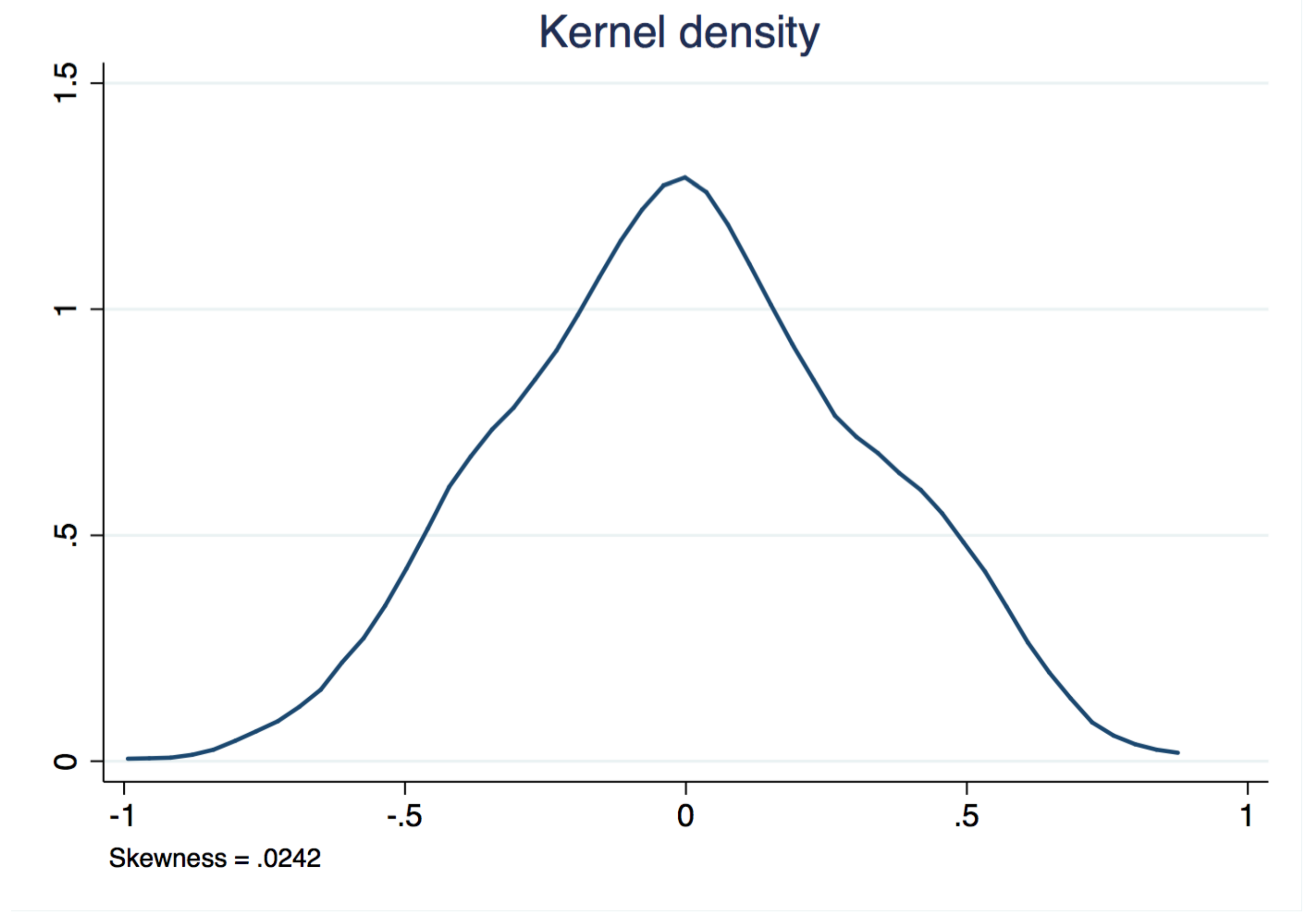
The study employs an unbalanced panel dataset of 39 developing countries ($i=1,\cdots ,39$) over the period 1989 to 2008 ($t=1989,\cdots ,2008$). Countries are selected following the IMF classification for developed and developing counties according to [49] and represented in

Table 2. Panel of 39 developing countries used in the analysis.

Country Name	ISO-Code	Geographic Specification
Albania	ALB	Europe
Algeria	DZA	Africa
Argentina	ARG	Latin America
Armenia	ARM	Commonwealth of Independent States
Azerbaijan	AZE	Commonwealth of Independent States
Belarus	BLR	Commonwealth of Independent States
Bolivia	BOL	Latin America
Botswana	BWA	Africa
Brazil	BRA	Latin America
Bulgaria	BGR	Europe
China	CHN	Asia
Congo	COG	Africa
Costa Rica	CRI	Latin America
Croatia	HRV	Europe
Egypt	EGY	Africa
El Salvador	SLV	Latin America
North Macedonia	MKD	Europe
Georgia	GEO	Commonwealth of Independent States
Honduras	HND	Latin America
India	IND	Asia
Indonesia	IDN	Asia
Iran	IRN	Middle East
Jordan	JOR	Middle East
Kazakhstan	KAZ	Commonwealth of Independent States
Kyrgyzstan	KGZ	Commonwealth of Independent States
Malaysia	MYS	Asia
Morocco	MAR	Africa
Nepal	NPL	Asia
Oman	OMN	Middle East
Pakistan	PAK	Middle East
Romania	ROU	Europe
Russia	RUS	Commonwealth of Independent States
Saudi Arabia	SAU	Middle East
South Africa	ZAF	Africa
Sri Lanka	LKA	Asia
Syria	SYR	Middle East
Thailand	THA	Asia
Tunisia	TUN	Africa
Uruguay	URY	Latin America

Note: Georgia is not a member of the Commonwealth of Independent States, but is included in this group for reasons of geography and similarity in economic structure.

while

Table 3. Descriptive statistics.

Variable	Label	Mean	Std. Dev.
Total final energy consumption ($ktoe$)	E	69,195	177,187
GDP (billion 2005 $USD$ using $PPPs$)	Y	426	975
Real consumer price index, energy	P	103	45
Population (millions)	$POP$	99	272
Agriculture, value added (% of $GDP$)	$ASH$	15	10
Industry value added (% of $GDP$)	$ISH$	35	10
Land area ($sq.km$)	A	1,500,114	3,135,589
Heating degree days * (base 70 °F)	$HDD$	18,668	15,288
Cooling degree days * (base 70 °F)	$CDD$	5798	4604

Note: * Heating degree days (HDD) and cooling degree days (CDD) are regarded as reliable variables for appropriately accounting for the effect of weather on energy-demand estimation [54]. HDD and CDD measure, respectively, how warm or cold a country is compared to the mean recorded outdoor temperature for a given country to a standard/base temperature. In this study, 70 °F is the base temperature for the HDD and the CDD to ensure that there are no non-zero values for some equatorial developing counties.

presents the descriptive statistics of the variables used in the analysis. The selection of the countries in the panel among the pool of developing countries is based initially on the availability of the data. Nonetheless, countries included in the panel should also meet criteria imposed as preliminary evidence of the existence of inefficiency use of energy. Indicators, such as electricity access and energy use per capita, were essential since countries with low access to electricity and low energy use per capita is more likely to underuse rather than overuse energy. Finally, skewness of the OLS residuals from the regression suggests the existence of the inefficient use of energy in the panel of the selected countries (Figure A1).

The dataset is based on information gathered from various sources. In particular, similar to many previous aggregate energy demand studies (such as [10]), the energy demand variable, E, is the aggregate total final energy consumption in thousand of tonnes equivalent (ktoe). The set of control variables include the standard economic drivers of energy demand used in previous energy demand studies (such as [10]); Y, which is GDP in billion 2005 US dollars in Purchasing Power Parity (PPP) and a real energy price variable, P, $2005=100$ as well as each country’s population, POP, in millions with E, Y, and POP collected from the IEA database [50] and P collected from International Labour Organisation Statistics [51]. Additionally, to control for economic structure and geographical size, variables for agricultural value added, ASH, industry value added, ISH, respectively, and land area, A in square kilometres (sq. km) are included with the data collected from the World Bank database [52]. Finally, to control for the influences of the different climate conditions, heating degree days (HDD) and cooling degree days (CDD) variables are included with the data taken from the King Abdullah Petroleum Studies and Research Centre (KAPSARC) dataset [53].

Following [48], SFA has been the subject of a great body of literature, resulting in many proposed econometric models to estimate cost and production functions, as described in Table 1. Among others, Pitt and Lee [39] adapt the original pooled model proposed for panel data and they propose the Random Effects model (REM) that interprets any unobserved, individual specific, time invariant heterogeneity as inefficiency. REM estimates efficiency scores that are constant over time and, hence, intuitively, REM tends to provide information about persistent efficiency. However, a crucial advantage that panel data models can offer, namely the control of unobserved heterogeneity is overlooked in REM. Contrariwise, Greene [40] extends the panel data version of the original model proposed by [48] by adding individual specific time-invariant effects and, thus, separating the unobserved time-invariant heterogeneity from time-varying efficiency. In this model, called the True Random Effects model (TREM), any time invariant inefficiency is completely absorbed by the individual specific term and therefore estimated efficiencies tend to provide information about the transient component of efficiency. Additionally, Filippini and Greene [19] propose a model called Generalised True Random Effects model (GTREM) that uses a maximum simulated likelihood approach for the estimation of Equation (2) and provides segregated estimations for the persistent and the transient component of efficiency from the same model, hereafter TGTREM and PGTREM, respectively.

The level of energy efficiency can be estimated using the conditional mean of the efficiency term proposed by [55] as follows:

$$E{F}_{it}=\frac{E_{it}^F}{E_{it}}=exp\{-{\widehat{u}}_{it}\}$$

where $E_{it}^F$ is the frontier energy demand and $E_{it}$ is the observed energy demand of each country in year t. Efficiency scores closer to unity indicate that countries utilise energy in a rational and efficient way while moving away from unity to zero countries waste energy.

Furthermore, Farsi et al. [41] argue that RE estimators can be affected by heterogeneity bias as it is possible that the unobserved country specific characteristics may not be distributed independently of the explanatory variables and they propose that the use of the Mundlak adjustment with the REM and TREM to confine the bias in inefficiency estimates by separating inefficiency from the unobserved heterogeneity and, thus, improving efficiency estimates. The Mundlak adjustment [56] of the REM considers the correlation of the country specific effects and the explanatory variables in an auxiliary equation as shown in

Table 4. Econometric specification of stochastic energy demand frontier: country specific effects, error term, and inefficiency.

	Model I	Model II	Model III
	MREM	TREM	GTREM
Country’s effects ${\alpha }_i$	${\alpha }_i=\gamma {\overline{X}}_{it}+{\delta }_i$	$N(\alpha ,{\sigma }_w^2)$	$N(\alpha ,{\sigma }_w^2)$
	${\displaystyle {\overline{X}}_{it}={\displaystyle \frac{1}{T}}\sum _{t=1}^T{X}_{it}}$
Full random error ${\epsilon }_{it}$	${\epsilon }_{it}={\delta }_i+v_{it}$	${\epsilon }_{it}=w_i+u_{it}+v_{it}$	${\epsilon }_{it}=w_i+h_{it}+u_{it}+v_{it}$
	${\delta }_i\sim N^{+}(0,{\sigma }_{\delta }^2)$	$u_{it}\sim N^{+}(0,{\sigma }_u^2)$	$u_{it}\sim N^{+}(0,{\sigma }_u^2)$
	$v_{it}\sim N(0,{\sigma }_v^2)$	$v_{it}\sim N(0,{\sigma }_v^2)$	$v_{it}\sim N(0,{\sigma }_v^2)$
		$w_i\sim N(0,{\sigma }_w^2)$	$w_i\sim N(0,{\sigma }_w^2)$
			$h_i\sim N(0,{\sigma }_h^2)$
Persistent inefficiency estimator	$E\left({\delta }_i\right|{\delta }_i+v_{it})$	∅	$E\left(h_i\right|{\epsilon }_{it})$
Transient inefficiency estimator	∅	$E\left(u_{it}\right|{\epsilon }_{it})$	$E\left(u_{it}\right|{\epsilon }_{it})$

, where ${\overline{X}}_{it}$ is a vector of the averages of explanatory variables and $\gamma$ is the respective vector of coefficients. The use of the Mundlak adjusment is also supported by [10,15,16,20,21].

Given the discussion above, three alternative models are employed for the estimation of Equation (2) in an attempt not only to estimate the level of ‘true’ energy efficiency in developing countries but to also evaluate the persistent and the transient counterparts of inefficiencies. Three basic models, namely the REM, TREM, and the GTREM, along with their Mundlak variations (i.e., MREM, MTREM, MGTREM) were tested; however, only the results of the three preferred models are presented here. Full details about the model specifications and estimated results, including all the models used are presented in

Table A1. Econometric specification of SEDF: effects, error term and inefficiency.

	REM	MREM	TREM	MTREM	GTREM	MGTREM
Country’s effects ${\alpha }_i$	$\alpha$	$$\begin{gathered} {\alpha }_i= \\ \gamma {\overline{X}}_{it}+{\delta }_i \end{gathered}$$	$N(\alpha ,{\sigma }_w^2)$	$$\begin{gathered} {\alpha }_i= \\ \gamma {\overline{X}}_{it}+w_i \end{gathered}$$	$N(\alpha ,{\sigma }_w^2)$	$$\begin{gathered} {\alpha }_i= \\ \gamma {\overline{X}}_{it}+w_i \end{gathered}$$
		$$\begin{gathered} {\displaystyle {\overline{X}}_{it}= \\ \frac{1}{T}{\displaystyle \sum _{t=1}^T}{X}_{it}} \end{gathered}$$		$$\begin{gathered} {\overline{X}}_{it}= \\ \frac{1}{T}{\displaystyle \sum _{t=1}^T}{X}_{it} \end{gathered}$$		$$\begin{gathered} {\displaystyle {\overline{X}}_{it}= \\ \frac{1}{T}\sum _{t=1}^T{X}_{it}} \end{gathered}$$
Full random error ${\epsilon }_{it}$	$\epsilon =u_i+v_{it}$	$$\begin{gathered} {\epsilon }_{it}= \\ {\delta }_i+v_{it} \end{gathered}$$	$$\begin{gathered} {\epsilon }_{it}=w_i+ \\ {u}_{it}+v_{it} \end{gathered}$$	$$\begin{gathered} {\epsilon }_{it}=w_i+ \\ {u}_{it}+v_{it} \end{gathered}$$	${\epsilon }_{it}=w_i+h_i+u_{it}+v_{it}$	${\epsilon }_{it}=w_i+h_i+u_{it}+v_{it}$
	$$\begin{gathered} u_i\sim \\ {N}^{+}(0,{\sigma }_u^2) \end{gathered}$$	$$\begin{gathered} {\delta }_i\sim \\ {N}^{+}(0,{\sigma }_{\delta }^2) \end{gathered}$$	$$\begin{gathered} u_{it}\sim \\ {N}^{+}(0,{\sigma }_u^2) \end{gathered}$$	$$\begin{gathered} u_{it}\sim \\ {N}^{+}(0,{\sigma }_u^2) \end{gathered}$$	$$\begin{gathered} u_{it}\sim \\ {N}^{+}(0,{\sigma }_u^2) \end{gathered}$$	$$\begin{gathered} u_{it}\sim \\ {N}^{+}(0,{\sigma }_u^2) \end{gathered}$$
	$$\begin{gathered} v_{it}\sim \\ N(0,{\sigma }_v^2) \end{gathered}$$	$$\begin{gathered} v_{it}\sim \\ N(0,{\sigma }_v^2) \end{gathered}$$	$$\begin{gathered} v_{it}\sim \\ N(0,{\sigma }_v^2) \end{gathered}$$	$$\begin{gathered} v_{it}\sim \\ N(0,{\sigma }_v^2) \end{gathered}$$	$$\begin{gathered} v_{it}\sim \\ N(0,{\sigma }_v^2) \end{gathered}$$	$$\begin{gathered} v_{it}\sim \\ N(0,{\sigma }_v^2) \end{gathered}$$
			$$\begin{gathered} w_i\sim \\ N(0,{\sigma }_w^2) \end{gathered}$$	$$\begin{gathered} w_i\sim \\ N(0,{\sigma }_w^2) \end{gathered}$$	$$\begin{gathered} w_i\sim \\ N(0,{\sigma }_w^2) \end{gathered}$$	$$\begin{gathered} w_i\sim \\ N(0,{\sigma }_w^2) \end{gathered}$$
					$$\begin{gathered} h_i\sim \\ N(0,{\sigma }_h^2) \end{gathered}$$	$$\begin{gathered} h_i\sim \\ N(0,{\sigma }_h^2) \end{gathered}$$
Persistent inefficiency estimator	$E\left(u_i\right|{\epsilon }_{it})$	$$\begin{gathered} E\left({\delta }_i\right|{\delta }_i+ \\ {v}_{it}) \end{gathered}$$	∅		$E\left(h_i\right|{\epsilon }_{it})$	$E\left(h_i\right|{\epsilon }_{it})$
Transient inefficiency estimator		∅	$E\left(u_{it}\right|{\epsilon }_{it})$	$E\left(u_{it}\right|{\epsilon }_{it})$	$E\left(u_{it}\right|{\epsilon }_{it})$	$E\left(h_i\right|{\epsilon }_{it})$

REM proposed by [39] considers the individual random effects as inefficiency rather than unobserved heterogeneity as in the traditional random effects model. Hence, estimation results of the REM provide information on the persistent part of the inefficiency in the use of energy. One drawback of this model is that any time-invariant individual-specific unobserved heterogeneity is considered inefficiency. Therefore, this REM tends to overestimate the level of ‘persistent’ inefficiency in the use of energy. In MREM, as proposed by [41], the unobserved heterogeneity bias problem is solved (at least partially) since the time-invariant unobserved heterogeneity is captured by the coefficients of the group mean of the time-varying explanatory variables of the Mundlak adjustment and not by the inefficiency component. Therefore, it is expected that the level of estimated energy efficiency obtained with MREM to be higher than the one obtained with REM. Estimation results confirm this point, as illustrated in Table 7. In TREM, the constant term, a in Equation (2), is substituted with a series of individual-specific random effects that take into account all unobserved socioeconomic and environmental characteristics that are time-invariant. Thus, TREM distinguishes the time-invariant unobserved heterogeneity w_i from the time varying level of efficiency component u_it. However, any time-invariant or persistent component of inefficiency is completely absorbed in the individual-specific constant terms. Therefore, generally TREM provide information only for the transient energy efficiency. Finally, for the REM and TREM, energy efficiency is estimated as shown in [55]. The GTREM gives the possibility to estimate simultaneously the persistent and transient part of inefficiency and is obtained by adding to the TREM a time persistent inefficiency component h_i. Therefore, this model considers a four-part disturbance with two-time varying components and two time-invariant components. Additionally, h_i, captures the persistent inefficiency in the use of energy while u_it captures the transient inefficiency. Finally, Filippini and Greene [19] develop a straightforward empirical estimation method which is followed in this thesis. The model is essentially a TREM consists of two part disturbance, one time varying (v_it + u_it) and one time invariant (w_i + h_i), in which each of the two parts has its own skew normal distribution rather than normal distribution. The computation of energy efficiency requires a one time, post estimation application of GHK simulation and NLOGIT5 econometric software is used for the estimations of all models.

and

Table A2. Summary of SFA studies on energy efficiency.

	REM		MREM	TREM		MTREM	GTREM
		Main Equation	Mundlak		Main Equation	Mundlak
Constant	$6.{804}^{***}$	$9.{754}^{***}$		$6.{074}^{***}$	$6.{985}^{***}$		$4.{158}^{***}$
	(1.605)	(3.692)		(0.094)	(0.159)		(0.119)
${\alpha }^y$	$0.{585}^{***}$	$0.{586}^{***}$	$0.{383}^{*}$	$0.{515}^{***}$	$0.{502}^{***}$	$0.{453}^{***}$	$0.{578}^{***}$
	(0.021)	(0.034)	(0.215)	(0.011)	(0.023)	(0.027)	(0.013)
${\alpha }^p$	$-0.{187}^{***}$	$-0.{172}^{***}$	$0.104$	$-0.{213}^{***}$	$-0.{197}^{***}$	$-0.{155}^{***}$	$-0.{221}^{***}$
	(0.014)	(0.017)	(0.525)	(0.008)	(0.010)	(0.051)	(0.010)
${\alpha }^{pop}$	$0.{581}^{***}$	$0.920$	$-0.{652}^{**}$	$0.{495}^{***}$	$0.{808}^{***}$	$1.{610}^{***}$	$0.{333}^{***}$
	(0.059)	(0.060)	(0.286)	(0.010)	(0.050)	(0.0051)	(0.011)
${\alpha }^a$	$0.111$	$-0.108$		$0.{030}^{***}$	$-0.{025}^{***}$		$0.{115}^{***}$
	(0.109)	(0.136)		(0.005)	(0.005)		(0.005)
${\alpha }^{hdd}$	$6.804$	$0.027$	$-0.078$	$0.{017}^{***}$	$0.020$	$-0.007$	$0.{050}^{***}$
	(0.039)	(0.047)	(0.103)	(0.003)	(0.039)	(0.039)	(0.003)
${\alpha }^{cdd}$	$0.062$	$-0.029$	$-0.{409}^{**}$	$-0.{046}^{***}$	$-0.032$	$-0.{251}^{***}$	$0.004$
	(0.047)	(0.075)	(0.171)	(0.007)	(0.035)	(0.036)	(0.008)
${\alpha }^{ish}$	$0.{002}^{***}$	$0.000$	$-0.003$	$0.{002}^{***}$	$0.001$	$-0.{002}^{**}$	$0.{004}^{***}$
	(0.001)	(0.001)	(0.009)	(0.000)	(0.001)	(0.001)	(0.000)
${\alpha }^{ash}$	$0.{006}^{***}$	$0.{005}^{***}$	$-0.011$	$0.{004}^{***}$	$0.{004}^{***}$	0.001	$0.{008}^{***}$
	(0.001)	(0.002)	(0.020)	(0.001)	(0.001)	(0.001)	(0.001)
${\alpha }^t$	$-0.002$	$-0.{012}^{***}$		$0.{011}^{***}$	$0.002$		$0.{010}^{***}$
	(0.003)	(0.004		(0.002)	(0.002)	(0.075)	(0.002)
${\alpha }^{t^2}$	$0.000$	$0.{001}^{**}$		$-0.{001}^{**}$	$0.000$		$-0.001$
	(0.000)	(0.000)		(0.000)	(0.000)	(0.075)	(0.000)
$\lambda$	$7.{071}^{*}$	$4.{381}^{*}$		$2.{901}^{***}$	$2.{061}^{***}$		$-0.001$
	(4.191)	(2.531)		(0.248)	(0.243)	(0.075)	(0.000)

Note: *** Significant at 1% level, ** Significant at 5% level, * Significant at 10% level. Standard errors are in parentheses. The sample includes 640 observations. NLOGIT5 econometric software is used for the estimations. GTREM with Mundlak modification does not converge.

in Appendix A. The Mundlak adjustment appears to control, at least partially, the heterogeneity in the REM and, thus, the MREM was preferred over the REM. However, concerning the TREM and the GTREM, the estimated parameter coefficients, as well as the efficiency scores were highly correlated with those produced by the respective Mundlak variations, but it seems that the introduction of a Mundlak modification in these models renders some of the variables statistically insignificant. For that reason, TREM and GTREM were preferred over the MTREM and the MGTREM. As explained previously, the REM with a Mundlak adjustment (MREM) provides estimations of energy efficiency that remain constant over time. For that reason, the literature suggest that this model tends to give information about the persistent energy efficiency of a country [20]. The second model used in this study is the TREM that gives information about the transient efficiency while, finally, the GTREM is used to estimate both components (persistent and transient) of inefficiency. Table 4 provides detailed econometric specifications of these models.

5. Empirical Results and Discussion

The estimation results of the aggregate energy demand frontier models, detailed in the previous sections, are given in

Table 5. Estimation results.

	MREM		TREM	GTREM
	Main Equation	Mundlak
Constant	$9.{754}^{***}$		$6.{074}^{***}$	$4.{158}^{***}$
	(3.692)		(0.094)	(0.119)
${\alpha }^y$	$0.{586}^{***}$	$0.{383}^{*}$	$0.{515}^{***}$	$0.{578}^{***}$
	(0.034)	(0.215)	(0.011)	(0.013)
${\alpha }^p$	$-0.{172}^{***}$	$0.104$	$-0.{213}^{***}$	$-0.{221}^{***}$
	(0.017)	(0.525)	(0.008)	(0.010)
${\alpha }^{pop}$	$0.920$	$-0.{652}^{**}$	$0.{495}^{***}$	$0.{333}^{***}$
	(0.060)	(0.286)	(0.010)	(0.011)
${\alpha }^a$	$-0.108$		$0.{030}^{***}$	$0.{115}^{***}$
	(0.136)		(0.005)	(0.005)
${\alpha }^{hdd}$	$0.027$	$-0.078$	$0.{017}^{***}$	$0.{050}^{***}$
	(0.047)	(0.103)	(0.003)	(0.003)
${\alpha }^{cdd}$	$-0.029$	$-0.{409}^{**}$	$-0.{046}^{***}$	$0.004$
	(0.075)	(0.171)	(0.007)	(0.008)
${\alpha }^{ish}$	$0.000$	$-0.003$	$0.{002}^{***}$	$0.{004}^{***}$
	(0.001)	(0.009)	(0.000)	(0.000)
${\alpha }^{ash}$	$0.{005}^{***}$	$-0.011$	$0.{004}^{***}$	$0.{008}^{***}$
	(0.002)	(0.020)	(0.001)	(0.001)
${\alpha }^t$	$-0.{0116}^{***}$		$0.0111^{***}$	$0.0101^{***}$
	(0.004)		(0.002)	(0.002)
${\alpha }^{t^2}$	$0.{0004}^{**}$		$-0.{0002}^{**}$	$-0.0001$
	(0.000)		(0.000)	(0.000)
$\lambda$	$4.{381}^{*}$		$2.{901}^{***}$	$1.{550}^{***}$
	(2.531)		(0.248)	(0.171)
$\sigma$	$0.{529}^{***}$		$0.{183}^{***}$	$0.{169}^{***}$
			(0.003)	(0.005)
Log Likelihood	374.361		366.791	346.230

Note: *** Significant at 1% level, ** Significant at 5% level, * Significant at 10% level. Standard errors are in parentheses. Coefficients of the time trend variables are given to four decimal places given they are relatively small. The sample includes 640 observations. NLOGIT5 econometric software is used for the estimations.

. The majority of the estimated coefficients, which for the variables in logarithmic form can be interpreted directly as elasticities of energy demand, appear to have the expected sign and almost all are statistically significant in the TREM and the GTREM. Furthermore, estimates of $\lambda$ are also given in Table 5. ($\lambda ={\sigma }_u/{\sigma }_v$ and provides information regarding the relative contribution of the two components of the error term so that an estimate of $\lambda$ closer to zero indicates that the disturbance noise is the dominant component whereas a nearly infinite estimate of $\lambda$ indicates that the compound error term is dominated by the one-sided error component). The estimated $\lambda$’s are all greater than one (>1) and statistically significant, demonstrating that the one-sided error component is relatively large in all models indicating that there is a considerable amount of estimated energy inefficiency in the models.

The results suggest that energy demand in developing countries is income and price inelastic. In particular, the estimated income elasticity of demand varies from 0.52 in the TREM to 0.59 in the REM while the estimated income elasticity in the GTREM lies betwixt at 0.58. The estimated own price elasticity of demand varies from −0.17 in the MREM to approximately −0.22 in both the TREM and the GTREM. Additionally, population appears to have positive influence on the energy demand. Namely, the estimated population elasticity is 0.92 but insignificant in the MREM while in the TREM and GTREM population elasticity is notably lower at 0.50 and 0.33, respectively, and both are statistically significant. The area coefficient is not significant in the MREM but suggests a positive and significant impact on the energy demand in both the TREM and the GTREM with the respective elasticities being at 0.30 and 0.11. Furthermore, the two climate variables are not significant in the MREM while the influence of HDD and CDD on the energy demand appear to be significant and positive in the TREM and the GTREM. A possible explanation for these results is that heating and/or cooling systems have yet to be widely used in developing countries.

As expected, the estimated coefficients of the shares of the industrial and the agricultural sector are positive, noting that the reference sector is the less energy intensive services sector. Finally, the UEDT is given by the first differential with respect to t of Equation (2), i.e., $a^t+2a^{t^2}t$. For the MREM, the estimated coefficient of the linear component (at) is negative and statistically significant whereas the quadratic component ($a^{t^2}$) is positive and statistically significant suggesting that the estimated UEDT has a relatively strong positive impact on energy demand. The positive impact of the UEDT possibly reflects an increasing appetite for energy services in developing countries that overcomes any potential benefits from the use of new technologies. It is also likely that the rate of adoption of technologies available in developing countries is quite slow, something that is mirrored in the relatively small estimated efficiency scores compared to results for developed countries in [10,16].

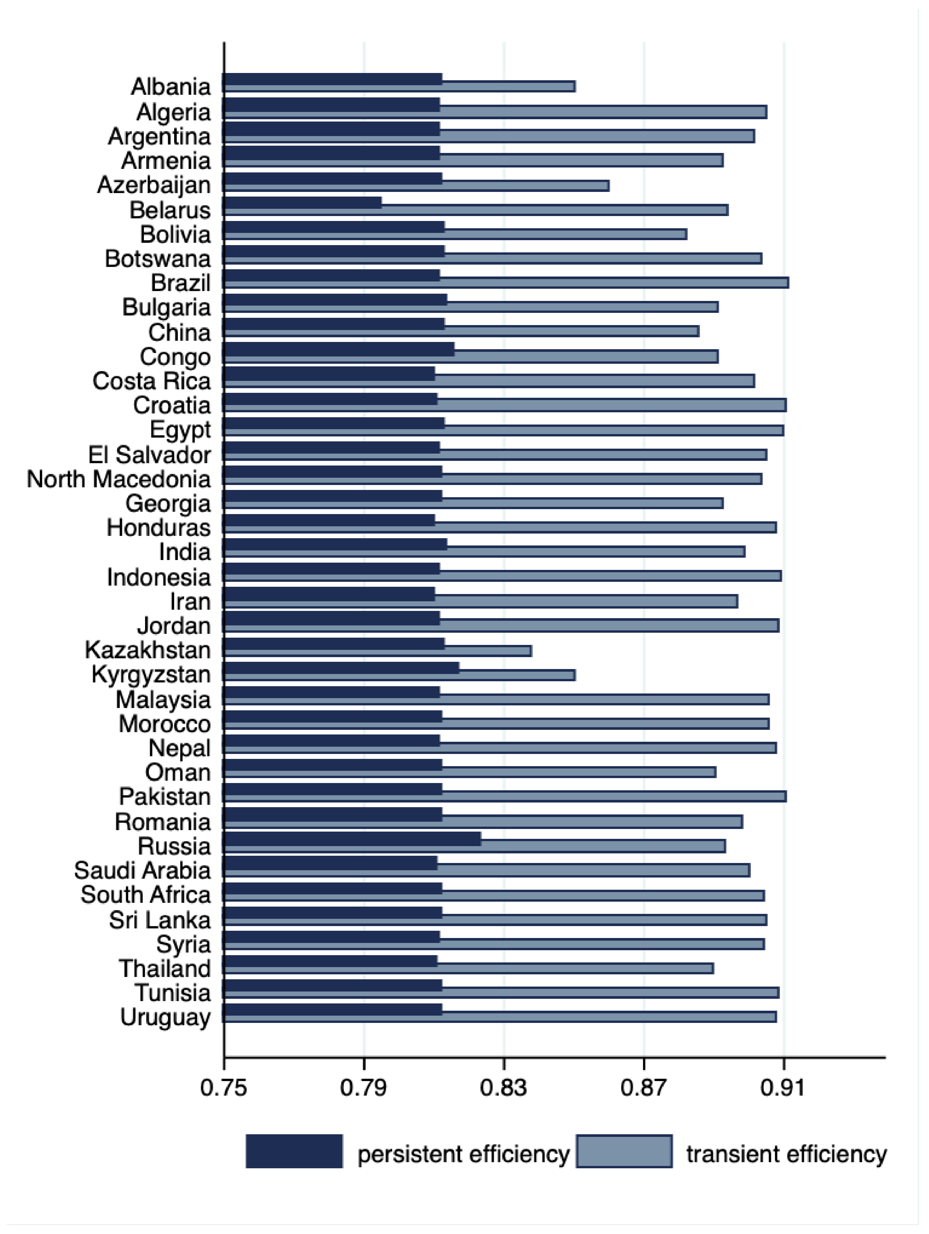
However, the main focus of SFA is not the estimation of the goal function (i.e., energy demand function) but the estimation of efficiency scores.

Table 6. Descriptive statistics of the estimated energy efficiency scores.

Model	Mean	Std. Dev.	Min	Max
MREM	0.705	0.203	0.335	0.969
TREM	0.881	0.077	0.391	0.986
PGTREM	0.812	0.004	0.795	0.823
TGTREM	0.896	0.049	0.560	0.974

provides descriptive statistics of the energy efficiency estimates for the panel of 39 developing counties over the period 1989–2008, obtained from each econometric specification. The results suggest that the estimated average values of the persistent efficiency vary from 70.5% in the MREM to 81.2% in the persistent part of the GTREM (PGTREM) while the transient efficiency is around 89%. In particular, it is 88.1% in the TREM and 89.6% in the transient part of the GTREM (TGREM).

These results are in line with the estimated energy efficiency in [34] which were on average between 81% and 91%. However, it should be noted that using the input distance function approach they estimate the level of technical efficiency in the use of energy while in this study the use of energy demand function provides estimations of the overall energy efficiency (both technical and allocative). Therefore, comparisons between these two studies should consider this important difference. Additionally, SFA provides relative efficiency scores given the dataset used. The study by [34] uses a panel of data consisting of 55 OECD and non-OECD countries while this study applies a dataset for solely 39 developing counties. Again, any comparisons of relative efficiency scores and ranking should consider this aspect. On average the estimated transient energy efficiency found on this study is higher than the persistent energy efficiency, possibly reflecting the lack of necessary energy efficiency regulations in developing countries, structural problems in the production of energy services and any other permanent in character behavioural and managerial failures. This result is in line with both [26,28] highlighting the low contribution of structural effect in energy intensity.

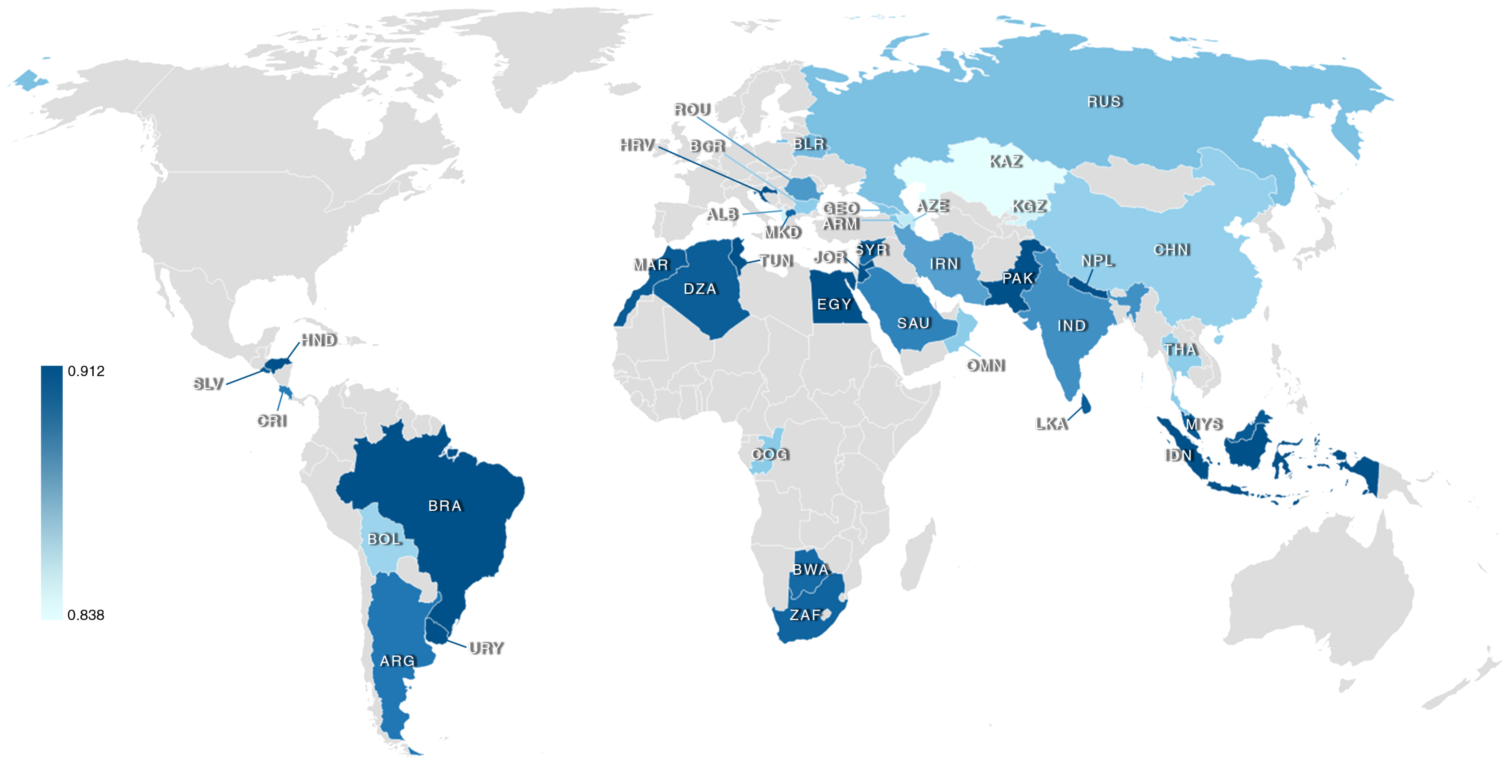
The correlation coefficient between the estimated values of the transient efficiency scores obtained with the TREM and the TGTREM, as illustrated in

Table 7. Correlation coefficients for the estimated energy efficiency scores and energy intensity.

	MREM	TREM	PGTREM	TGTREM	EI
MREM	1
TREM	0.045	1
PGTREM	0.075	−0.009	1
TGTREM	0.048	0.971	−0.054	1
EI	−0.460	−0.357	−0.006	−0.354	1

Note: Table provides the simple correlation coefficients of the estimates of the efficiency scores for the whole panel of 39 developing countries over the period 1989–2008 generated from the modelling and the energy intensity (EI—the ratio between energy consumption and gross domestic product).

, is very high at 0.97, highlighting that both models provide sufficient information regarding the transient energy efficiency. On the contrary, the value of the correlation coefficient between the estimated values of the persistent efficiency scores obtained from the MREM and the PGTREM is very low at 0.07 suggesting that the REM may not be a satisfactory indicator of persistent efficiency. A possible explanation for this, is that the REM considers any unobserved time-invariant country specific heterogeneity as inefficiency and thus produces lower efficiency scores. Overall, the preferred model is the GTREM which provides estimates for both the persistent and the transient energy efficiency. Hence, the analysis hereafter is based on the estimations of this model. Figure 1 presents the average transient and persistent energy efficiency by country, while Figure 2 illustrates the map of the countries in the panel given the estimated average value of their transient energy efficiency.

Furthermore, as expected, the estimated values of ‘true’ energy efficiency scores are negatively correlated with energy intensity and the correlation coefficients vary from −0.01 to −0.46. It is argued by [10,15] that the technique used here tends to provide useful information and can be an important tool for policy makers as long as the estimated efficiencies are not perfect or near perfectly correlated with energy intensity since then, all the necessary information would be gathered from the energy intensity. Nevertheless, this is not the case in this study. This result suggests that energy intensity is a poor proxy of energy efficiency for the developing countries and unless the kind of analysis employed here is undertaken it is possible that policy makers would have a misleading picture of the ‘true’ energy efficiency potential — a result that is also consistent with [10,15].

Table 8. Each country’s average energy efficiency and energy intensity for the period 1989–2008, their rankings, and the correlation coefficients between them.

Country	Average ‘True’ Energy Efficiency (TGTREM)		Average Energy Intensity (Toe per Thousand 2005 USD PPP)		Cor. Coef.
	Value	Rank	Value	Rank
Albania	0.850	38	0.095	15	−0.424
Algeria	0.905	15	0.055	3	−0.639
Argentina	0.902	20	0.120	22	−0.421
Armenia	0.893	29	0.130	24	−0.010
Azerbaijan	0.860	36	0.223	33	−0.336
Belarus	0.894	26	0.288	38	−0.391
Bolivia	0.882	35	0.105	18	−0.985
Botswana	0.904	19	0.086	9	−0.913
Brazil	0.912	1	0.088	10	0.555
Bulgaria	0.891	31	0.178	31	−0.879
China	0.886	34	0.245	35	−0.862
Congo	0.892	30	0.050	2	−0.907
Costa Rica	0.901	21	0.071	6	−0.809
Croatia	0.911	3	0.106	19	0.302
Egypt	0.910	4	0.073	7	0.090
El Salvador	0.905	13	0.089	13	−0.244
North Macedonia	0.904	18	0.110	21	−0.846
Georgia	0.893	28	0.184	32	−0.484
Honduras	0.908	9	0.145	27	−0.462
India	0.899	23	0.140	25	−0.917
Indonesia	0.909	5	0.108	20	−0.399
Iran	0.897	25	0.145	26	−0.640
Jordan	0.908	7	0.102	17	−0.383
Kazakhstan	0.838	39	0.250	37	−0.0698
Kyrgyzstan	0.851	37	0.241	34	−0.936
Malaysia	0.906	11	0.088	11	−0.942
Morocco	0.906	12	0.071	5	−0.656
Nepal	0.908	8	0.250	36	0.444
Oman	0.890	32	0.043	1	−0.987
Pakistan	0.911	2	0.122	23	−0.808
Romania	0.898	24	0.160	29	−0.613
Russia	0.894	27	0.317	39	−0.855
Saudi Arabia	0.901	22	0.089	12	−0.961
South Africa	0.904	16	0.153	28	−0.875
Sri Lanka	0.905	14	0.089	14	−0.481
Syria	0.904	17	0.178	15	−0.858
Thailand	0.890	33	0.099	16	−0.967
Tunisia	0.909	6	0.084	8	0.498
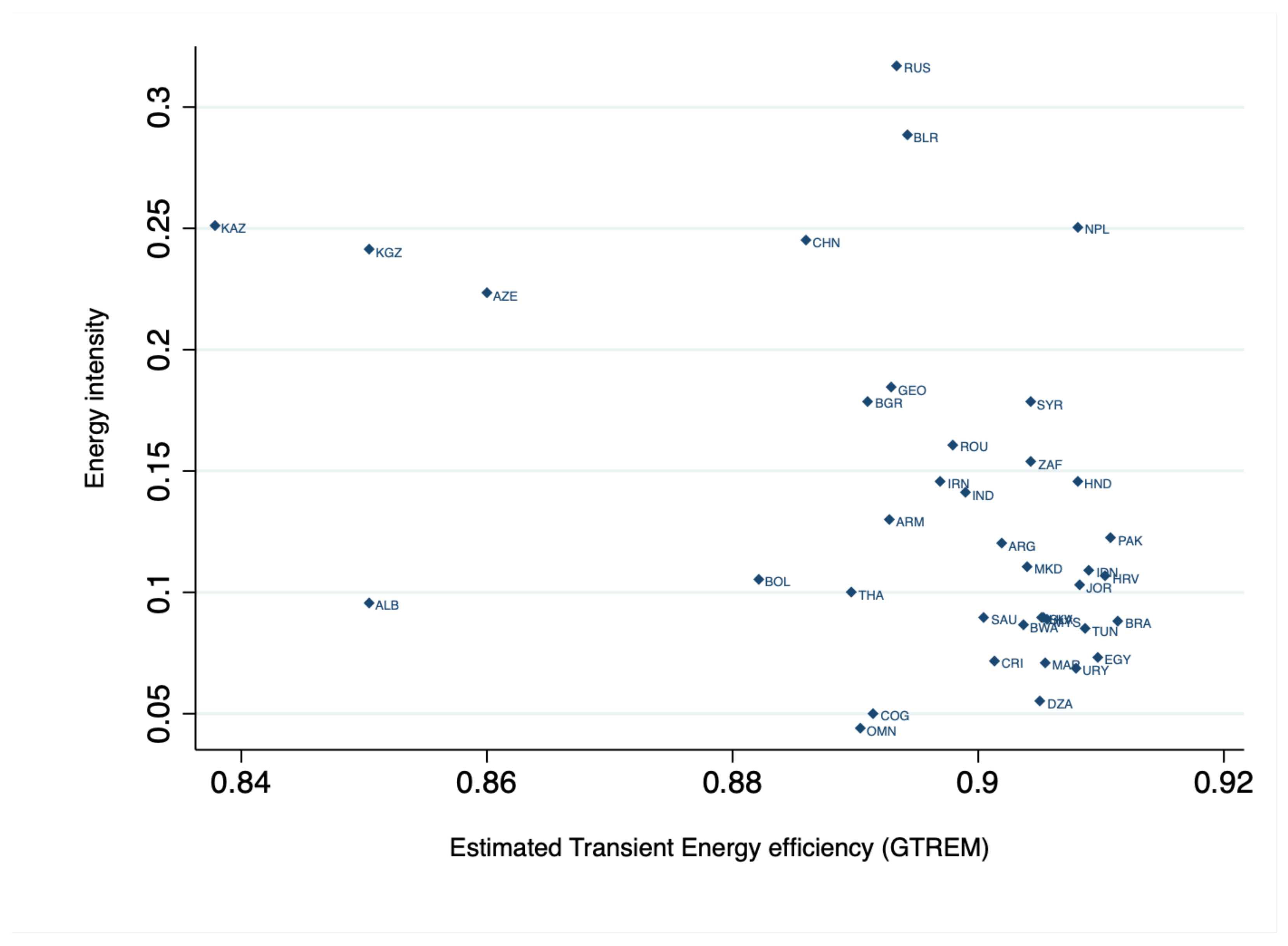
Uruguay	0.908	10	0.068	4	−0.687

provides the estimated average ‘true’ energy efficiency scores obtained from the TGTREM for each country and compares these values with the average energy intensity. Table 8 also provides the relative ranking of the countries in the panel with both measurements and shows that Brazil, Pakistan, Croatia, Egypt, and Indonesia are the most efficient countries using the TGTREM, while Bolivia, Azerbaijan, Kyrgyzstan, Albania, and Kazakhstan are the least efficient. On the other hand, energy intensity suggests that Oman, Congo, Algeria, Uruguay, and Morocco are the most efficient counties, and China, Nepal, Kazakhstan, Belarus, and Russia are the least efficient ones. Table 8 also illustrates that estimated energy efficiency is negatively correlated with energy intensity, as expected, since when energy efficiency increases energy intensity would generally be expected to decrease. However, this is not always the case. Some countries (i.e., Brazil, Croatia, Egypt, Nepal, and Tunisia) appear to have a positive relationship between the estimated energy efficiency and energy intensity. In addition, among the panel there are countries that have a strong negative correlation (>90%) between the estimated energy efficiency and energy intensity (i.e., Bolivia, Botswana, Congo, India, Kyrgyzstan, Malaysia, Oman, Saudi Arabia, and Thailand) while for some other countries (i.e., Armenia, Azerbaijan, Belarus, Croatia, Egypt, El Salvador, Indonesia, and Jordan) this correlation is significantly lower.

Additionally, for the period 1989–2008 according to the estimated TGTREM, Pakistan, Nepal, Costa Rica, Congo, and Oman are ranked 2nd, 8th, 21st, 30th, and 32nd, respectively, whereas they are ranked 23rd, 36th, 6th, 2nd, and 1st according to energy intensity measurement. Although there is a general negative relationship between estimated energy efficiency and energy intensity this is not one to one regarding the relative rankings. In addition, the Spearman rank correlation coefficient is equal $\rho \left(37\right)=0.35$ with p-value = 0.03. This relationship between two measurements is further illustrated in Figure 3.

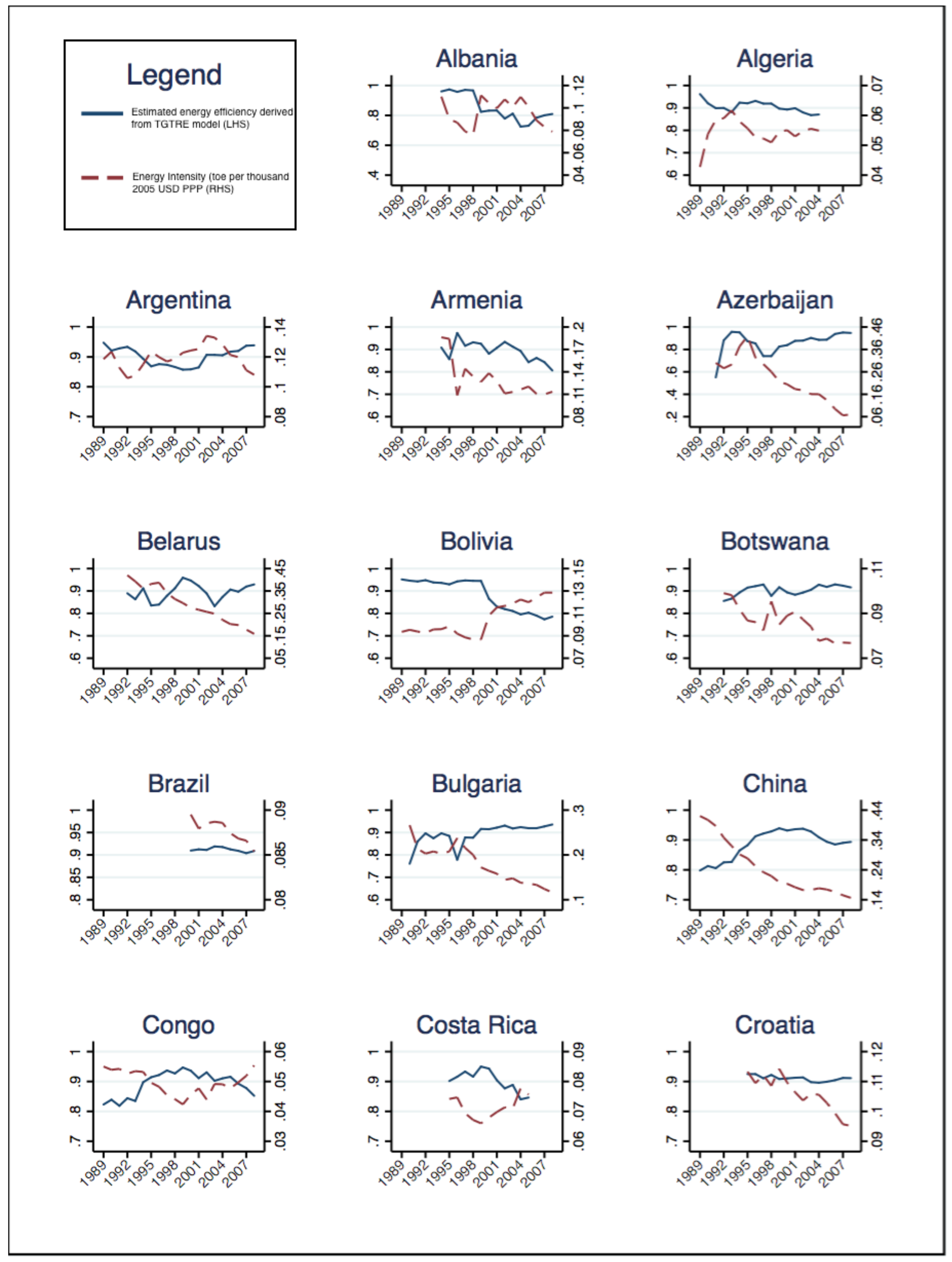
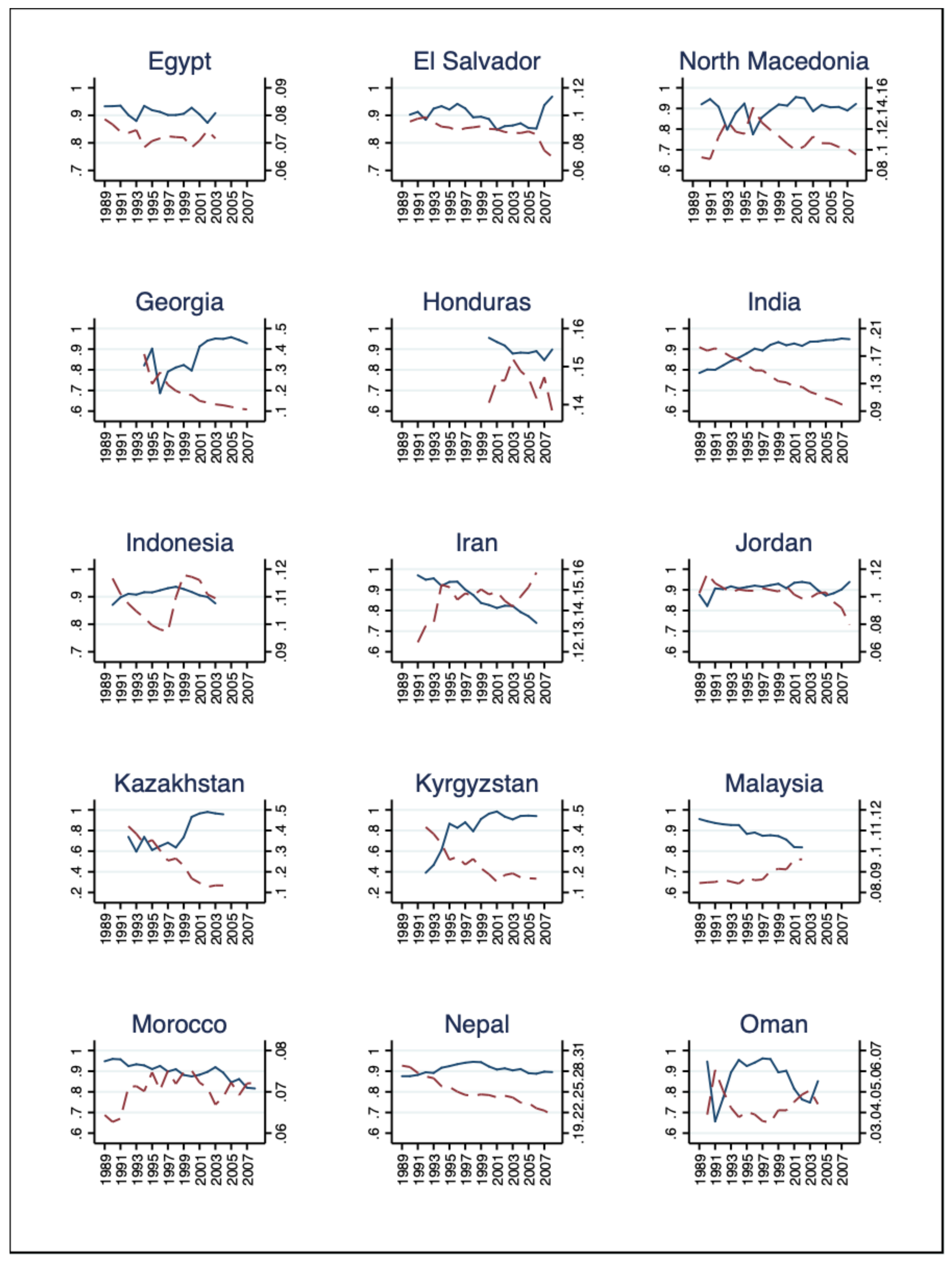
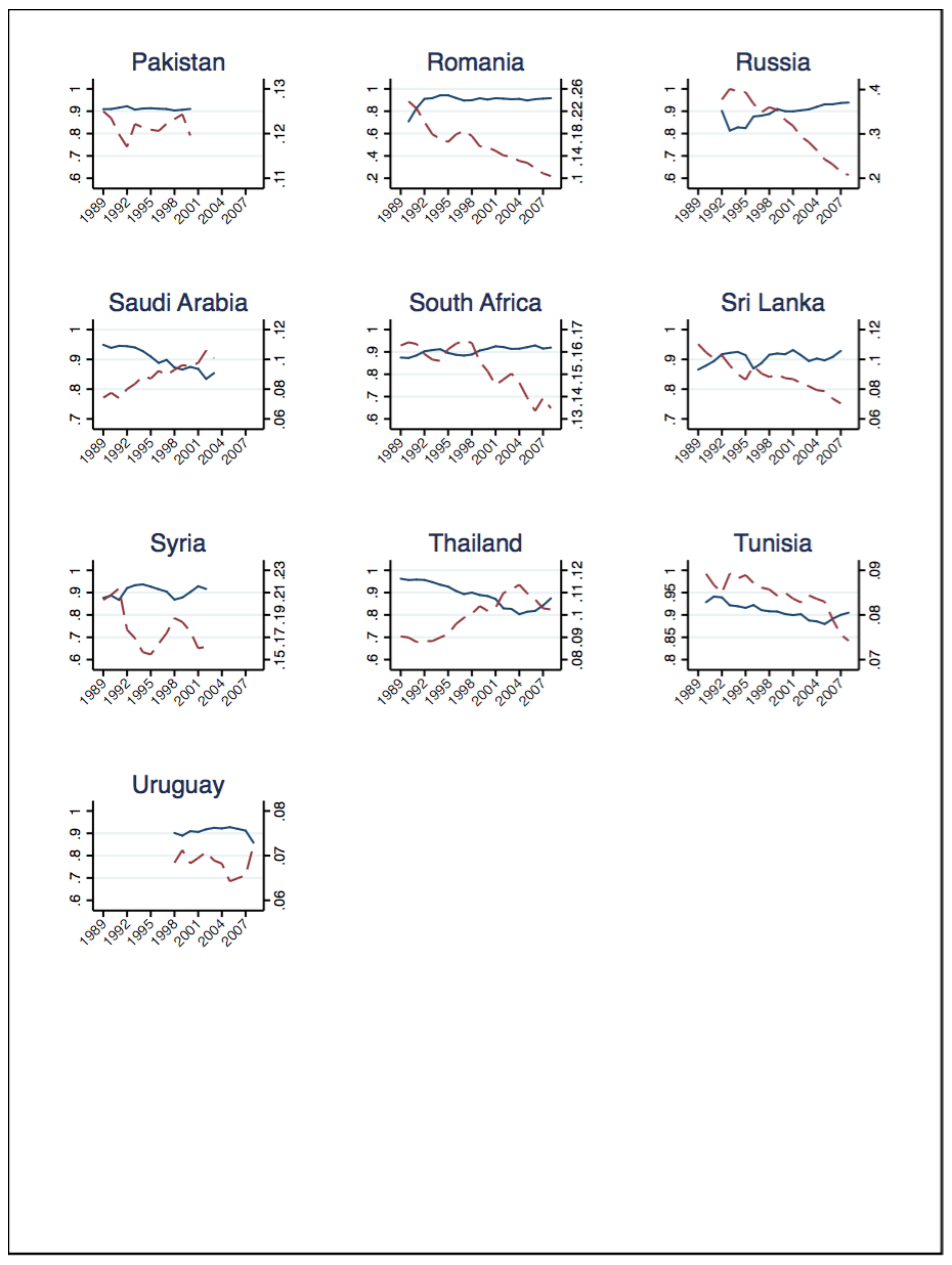
Figure 4 shows the comparison between the estimated transient energy efficiency and energy intensity of each country over the period 1989–2008. It should be noted that this study is based on an unbalanced panel dataset for the estimation of efficiency scores and for that reason some counties in Figure 4, such as Brazil and Honduras, are over a shorter period. Additionally, only the estimated transient energy efficiency is used for comparison with energy intensity since the correlation between these two measurements is −0.35 while the correlation between the persistent energy efficiency and the energy intensity is only −0.1. Another reason is that the estimated transient energy efficiency appears notable variation among the countries and over the estimated period while persistent efficiency is constant and there are no significant differences among the countries. Figure 4 also indicates that there is no clear, common trend regarding energy-efficiency improvements. In particular, some countries (i.e., Azerbaijan, Botswana, China, India, Kazakhstan, Kyrgyzstan, and Russia) clearly have improved their energy efficiency over the estimated period while some other countries (i.e., Albania, Algeria, Bolivia, Iran, Malaysia, Morocco, Saudi Arabia, Thailand, and Tunisia) display a downward sloping trend in energy efficiency. Finally, there is a group of countries where ‘true’ energy efficiency shows some level of fluctuation or is quite steady over the estimation period.

Given the discussion above, estimated energy efficiency tend to give more accurate information regarding energy efficiency of a country than energy intensity does and hence this study uses the term ‘true’ energy efficiency to describe the estimated energy efficiency scores and distinguish them from the energy intensity. It is worth noting that SFA is a benchmarking technique and, hence, each county’s estimated energy efficiency might not illustrate the precise country’s position. However, estimated energy efficiency measurements provide useful information regarding each country’s change in energy efficiency over the estimated period and allows for comparisons among the countries in the panel.

6. Conclusions

This paper uses an energy demand frontier model in order to estimate the ‘true’ energy efficiency for a sample of 39 developing countries over the period 1989–2008. The aggregate energy demand specification controls for income, price, population, area size, the share of the agricultural sector and the services sector in GDP, HDD, CDD and a UEDT, expressed by a quadratic time trend, and it is estimated using three alternative econometric techniques, namely the MREM, the TREM, and the GTREM. These alternative models represent different sources of information regarding the energy efficiency of a country and, thus, there is no absolute preferred model among them but a combination of these three could lead to useful conclusions. Overall, REM tend to estimate the level of persistent energy efficiency while the TREM estimates provide information regarding the transient energy efficiency. Finally, the GTREM allows for estimation of both persistent and transient energy efficiency simultaneously.

The estimated results indicate, as expected, that the transient and persistent counterparts are quite different in values and not highly correlated. This is because the sources of inefficiency are quite different. Therefore, policy makers should be informed about the levels of both transient and persistent energy efficiency to be able to design effective energy policies. The TGTREM estimates are very highly correlated with estimates produced by the TREM and, thus, both models could explain trends in transient energy efficiency. On the contrary, the correlation between the PGTREM estimates and the MREM is relatively lower. This is in line with previous literature which argues that in the REM all the time invariant variables are captured by the individual effects and, hence, the REM produces higher level of inefficiencies. The Mundlak adjustment seems to control part of this time invariant heterogeneity. (The correlation between the REM and the PGTREM is significantly lower than that between the MREM and the PGTREM suggesting that Mundlak modification controls, at least partially, the unobserved time invariant heterogeneity). The estimated results also suggest that there is a significant potential for energy saving in developing countries. In particular, persistent inefficiency, on average, is higher than the transient reflecting the potential lack of structural reforms of economies and the implementation of the necessary regulatory framework that would attract investments on the energy efficiency.

Additionally, the information from this study is of use to policy makers in developing countries and international organisations showing where energy intensity alone is likely not to be a good indicator of energy efficiency, thus possibly avoiding policy mistakes based purely on intensity. Furthermore, the results indicate to policy makers where there is significant potential for CO₂ emission savings if countries utilise energy efficiently. Generally, most efficient countries tend to use less energy but this is not always the case. Three countries, namely China, India, and Russia, which are among the world’s top-5 emitters appear to be quite inefficient in their use of energy. Although these countries have increased their respective level of energy efficiency during the examined period, there is still ample scope for improvements in energy efficiency. In the light of the Paris agreement, that consider both developed and developing countries equally responsible to design and implement national energy strategies in the direction of reducing their energy consumption and the associated CO₂ emissions by 2020, this result is particularly important from a policy-making perspective.

At the country level, estimated results are in line with previous studies suggesting great heterogeneity across countries’ efficiency scores. The majority of the countries have improved their energy efficiency over the estimated period. However, a group of countries, especially Latin America countries, appear to have a downward trend in their energy-efficiency scores or great volatility with no dominant trend. This arguably reflects the fact that developing countries have not been bound to implement environmentally sensitive energy strategies, until more recently. Finally, estimated energy efficiency is negatively correlated with energy intensity for most of the countries, as expected, but this negative correlation appears to have significant heterogeneity across countries varying from −0.01 to −0.99. In addition, for some countries the results indicate a positive relationship between the estimated ‘true’ energy efficiency and energy intensity, unveiling the weakness of using energy intensity or the energy consumption to GDP ratio as a proxy of energy efficiency—a result that is in line with previous literature. This study is based on the economic theory of production and after controlling for a range of economic and other factors, provides effective energy efficiency measurements that could offer an ancillary instrument to policy makers in order to avoid any potential misguided conclusions.

References

- IEA. Key World Energy Statistics 2021; Technical report; OECD: Paris, France; IEA: Paris, France, 2021. [Google Scholar]
- IEA. World Energy Outlook 2014; Technical report; OECD: Paris, France; IEA: Paris, France, 2014. [Google Scholar]
- UNIDO. Energy for a Sustainable Future; Technical report; United Nations for Industrial Development Organisation: Vienna, Austria, 2010. [Google Scholar]
- Kaczmarzewski, S.; Matuszewska, D.; Sołtysik, M. Analysis of Selected Service Industries in Terms of the Use of Photovoltaics before and during the COVID-19 Pandemic. Energies 2021, 15, 188. [Google Scholar] [CrossRef]
- IEA. Energy Efficiency Indicators Highlights 2016; Technical Report; OECD: Paris, France; IEA: Paris, France, 2016. [Google Scholar]
- IEA. Energy Efficiency 2022; Technical Report; IEA: Paris, France, 2022. [Google Scholar]
- Koval, V.; Borodina, O.; Lomachynska, I.; Olczak, P.; Mumladze, A.; Matuszewska, D. Model Analysis of Eco-Innovation for National Decarbonisation Transition in Integrated European Energy System. Energies 2022, 15, 3306. [Google Scholar] [CrossRef]
- IEA. For The first Time in Decades, the Number of People without Access to Electricity Is Set to Increase in 2022; Technical report; IEA: Paris, France, 2022. [Google Scholar]
- IEA. Progress with Implementing Energy Efficiency Policies in the G8; Technical report; OECD: Paris, France; IEA: Paris, France, 2009. [Google Scholar]
- Filippini, M.; Hunt, L.C. Energy Demand and Energy Efficiency in the OECD Countries: A Stochastic Demand Frontier Approach. Energy J. 2011, 32, 59–80. [Google Scholar] [CrossRef] [Green Version]
- Filippini, M.; Hunt, L.C. Measurement of energy efficiency based on economic foundations. Energy Econ. 2015, 52 (Suppl. 1), S5–S16. [Google Scholar] [CrossRef] [Green Version]
- Evans, J.; Filippini, M.; Hunt, L.C. The contribution of energy efficiency towards meeting CO2 targets. In Handbook on Energy and Climate Change; Fouquet, R., Ed.; Edward Elgar Publishing: Oxford, UK, 2013; Chapter 8; pp. 175–223. [Google Scholar]
- Huntington, H.G. Been top down so long it looks like bottom up to me. Energy Policy 1994, 22, 833–839. [Google Scholar] [CrossRef]
- Kopp, R.J. The Measurement of Productive Efficiency: A Reconsideration. Q. J. Econ. 1981, 96, 477–503. [Google Scholar] [CrossRef]
- Filippini, M.; Hunt, L.C. US residential energy demand and energy efficiency: A stochastic demand frontier approach. Energy Econ. 2012, 34, 1484–1491. [Google Scholar] [CrossRef] [Green Version]
- Filippini, M.; Hunt, L.; Zoric, J. Impact of energy policy instruments on the estimated level of underlying energy efficiency in the EU residential sector. Energy Policy 2014, 69, 73–81. [Google Scholar] [CrossRef] [Green Version]
- Otsuka, A.; Goto, M. Estimation and determinants of energy efficiency in Japanese regional economies. Reg. Sci. Policy Pract. 2015, 7, 89–101. [Google Scholar] [CrossRef]
- Alberini, A.; Filippini, M. Transient and persistent energy efficiency in the US residential sector: Evidence from household-level data. Energy Effic. 2015, 11, 589–601. [Google Scholar] [CrossRef]
- Filippini, M.; Greene, W. Persistent and transient productive inefficiency: A maximum simulated likelihood approach. J. Product. Anal. 2016, 45, 187–196. [Google Scholar] [CrossRef]
- Filippini, M.; Hunt, L.C. Measuring persistent and transient energy efficiency in the US. Energy Effic. 2016, 9, 663–675. [Google Scholar] [CrossRef] [Green Version]
- Filippini, M.; Zhang, L. Estimation of the energy efficiency in Chinese provinces. Energy Effic. 2016, 9, 1315–1328. [Google Scholar] [CrossRef]
- Lundgren, T.; Marklund, P.O.; Zhang, S. Industrial energy demand and energy efficiency-Evidence from Sweeden. Resour. Energy Econ. 2016, 43, 130–152. [Google Scholar] [CrossRef]
- Broadstock, D.C.; Li, J.; Zhang, D. Efficiency snakes and energy ladders: A (meta-) frontier demand analysis of electricity consumption efficiency in Chinese households. Energy Policy 2016, 91, 383–396. [Google Scholar] [CrossRef] [Green Version]
- Marin, G.; Palma, A. Technology invention and adoption in residential energy consumption: A stochastic frontier approach. Energy Econ. 2017, 66, 85–98. [Google Scholar] [CrossRef]
- Zhang, X.P.; Cheng, X.M.; Yuan, J.H.; Gao, X.J. Total-factor energy efficiency in developing countries. Energy Policy 2011, 39, 644–650. [Google Scholar] [CrossRef]
- Adom, P.K.; Amakye, K.; Abrokwa, K.K.; Quaidoo, C. Estimate of transient and persistent energy efficiency in Africa: A stochastic frontier approach. Energy Convers. Manag. 2018, 166, 556–568. [Google Scholar] [CrossRef]
- Kumbhakar, S.C.; Heshmati, A. Efficiency measurement in Swedish dairy farms: An application of rotating panel data, 1976–88. Am. J. Agric. Econ. 1995, 77, 660–674. [Google Scholar] [CrossRef]
- Sun, H.; Edziah, B.K.; Song, X.; Kporsu, A.K.; Taghizadeh-Hesary, F. Estimating persistent and transient energy efficiency in belt and road countries: A stochastic frontier analysis. Energies 2020, 13, 3837. [Google Scholar] [CrossRef]
- Cantore, N. Energy Efficiency in Developing Countries for the Manufacturing Sector; United Nations Industrial Development Organization: Vienna, Austria, 2011. [Google Scholar]
- Jimenez, R.; Mercado, J. Energy intensity: A decomposition and counterfactual exercise for Latin American countries. Energy Econ. 2014, 42, 161–171. [Google Scholar] [CrossRef] [Green Version]
- Voigt, S.; Cian, E.D.; Schymura, M.; Verdolini, E. Energy intensity developments in 40 major economies: Structural change or technology improvement? Energy Econ. 2014, 41, 47–62. [Google Scholar] [CrossRef] [Green Version]
- Boyd, G.A. Estimating Plant Level Energy Efficiency with a Stochastic Frontier. Energy J. 2008, 29, 23–43. [Google Scholar] [CrossRef]
- Zhou, P.; Ang, B.; Zhou, D. Measuring economy-wide energy efficiency performance: A parametric frontier approach. Appl. Energy 2012, 90, 196–200. [Google Scholar] [CrossRef]
- Adetutu, M.; Glass, A.; Weyman-Jones, T. Economy-wide Estimates of Rebound Effects: Evidence from Panel Data. Energy J. 2016, 37, 251–269. [Google Scholar] [CrossRef]
- Lin, B.; Du, K. Technology gap and China’s regional energy efficiency: A parametric metafrontier approach. Energy Econ. 2013, 40, 529–536. [Google Scholar] [CrossRef]
- Lin, B.; Wang, X. Exploring energy efficiency in China’s iron and steel industry: A stochastic frontier approach. Energy Policy 2014, 72, 87–96. [Google Scholar] [CrossRef]
- Lin, B.; Long, H. A stochastic frontier analysis of energy efficiency of China’s chemical industry. J. Clean. Prod. 2015, 87, 235–244. [Google Scholar] [CrossRef]
- Shen, X.; Lin, B. Total Factor Energy Efficiency of China’s Industrial Sector: A Stochastic Frontier Analysis. Sustainability 2017, 9, 646. [Google Scholar] [CrossRef] [Green Version]
- Pitt, M.M.; Lee, L.F. The measurement and sources of technical inefficiency in the Indonesian weaving industry. J. Dev. Econ. 1981, 9, 43–64. [Google Scholar] [CrossRef]
- Greene, W. Fixed and Random Effects in Stochastic Frontier Models. J. Product. Anal. 2005, 23, 7–32. [Google Scholar] [CrossRef] [Green Version]
- Farsi, M.; Filippini, M.; Kuenzle, M. Unobserved heterogeneity in stochastic cost frontier models: An application to Swiss nursing homes. Appl. Econ. 2005, 37, 2127–2141. [Google Scholar] [CrossRef]
- Battese, G.E.; Coelli, T.J. Frontier production functions, technical efficiency and panel data: With application to paddy farmers in India. In International Applications of Productivity and Efficiency Analysis; Springer: Berlin/Heidelberg, Germany, 1992; pp. 149–165. [Google Scholar]
- Battese, G.E.; Coelli, T.J. A model for technical inefficiency effects in a stochastic frontier production function for panel data. Empir. Econ. 1995, 20, 325–332. [Google Scholar] [CrossRef] [Green Version]
- Kumbhakar, S.C.; Lien, G.; Hardaker, J.B. Technical efficiency in competing panel data models: A study of Norwegian grain farming. J. Product. Anal. 2014, 41, 321–337. [Google Scholar] [CrossRef] [Green Version]
- Chen, Y.Y.; Schmidt, P.; Wang, H.J. Consistent estimation of the fixed effects stochastic frontier model. J. Econom. 2014, 181, 65–76. [Google Scholar] [CrossRef]
- Kumbhakar, S. Stochastic Frontier Analysis: An Econometric Approach; Cambridge University Press: Cambridge, UK, 2000. [Google Scholar]
- Hunt, L.C.; Judge, G.; Ninomiya, Y. Modelling underlying energy demand trends. In Energy in a competitive market: essays in honour of Colin Robinson; Hunt, L.C., Ed.; Edward Elgar: Cheltenham, UK, 2003; Chapter 9; pp. 140–174. [Google Scholar]
- Aigner, D.; Lovell, C.A.K.; Schmidt, P. Formulation and estimation of stochastic frontier production function models. J. Econom. 1977, 6, 21–37. [Google Scholar] [CrossRef]
- IMF. World Economic Outlook: Uneven Growth. Short-and Long-Term Factors; Technical report; International Monetary Fund: Washington, DC, USA, 2015. [Google Scholar]
- IEA. World Energy Balances: World Indicators; IEA: Paris, France, 2017; pp. 1960–2015. [Google Scholar]
- International Labour Organisation. ILOSTAT-ILO Database of Labour Statistics; International Labour Organization: Geneva, Switzerland, 2017. [Google Scholar]
- World Bank. World Development Indicators; World Bank: Washington, DC, USA, 2017. [Google Scholar]
- KAPSARC. A Global Degree Days Database for Energy-Related Applications; King Abdullah Petroleum Studies and Research Centre: Riyadh, Saudi Arabia, 2015. [Google Scholar]
- Atalla, T.; Gualdi, S.; Lanza, A. A global degree days database for energy-related applications. Energy 2018, 143, 1048–1055. [Google Scholar] [CrossRef] [Green Version]
- Jondrow, J.; Lovell, C.K.; Materov, I.S.; Schmidt, P. On the estimation of technical inefficiency in the stochastic frontier production function model. J. Econom. 1982, 19, 233–238. [Google Scholar] [CrossRef] [Green Version]
- Mundlak, Y. On the Pooling of Time Series and Cross Section Data. Econometrica 1978, 46, 69–85. [Google Scholar] [CrossRef]
- Kipouros, P. Energy Efficiency and The Rebound Effect in Developing Countries. Ph.D. Thesis, University of Surrey, Guildford, UK, 2017. (Unpublished Ph.D. Thesis). [Google Scholar]
Figure 1.
Estimated persistent and transient efficiency in developing countries.
Figure 2.
Energy efficiency in developing countries.
Figure 3.
Estimated average energy efficiency Vs. average energy intensity 1989–2008.
Figure 4.
Comparison of estimated ‘true energy efficiency with energy intensity by country.