Modelling of Automated Store Energy Consumption

Abstract

Over the last decade, a constantly growing trend of the popularization of self-service automated stores has been observed. Vending machines have been expanded into fully automated stores, the offer of which is comparable to small, conventional stores. One of the basic reasons for the popularization of modern automated stores is the reduction in a store’s energy consumption while ensuring a comparable range of products offered. The research into possibilities of reducing greenhouse gases emission is important in terms of the environment and climate protection. The research presented in the paper concerns the development of a model for determining electricity consumption, operating costs and CO₂ emission of an automated store designed and developed by Delfin company. In the developed model, the potential location of the store, prevailing climatic conditions and expected product sales are taken into account. Estimated energy demand for the store is the information of key importance for the potential investors and the manufacturer of the automated store. It is worth emphasizing that the average annual electrical energy consumption evaluated for a grocery store of an area of 70 m² amounted to approximately 38.4 MWh, while for an automated store of an area of 9 m² and a comparable product range, the electricity consumption was approximately 10.1 MWh, i.e., 74% smaller.

1. Introduction

Over the last decade, a constantly growing trend of the popularization of self-service automated stores has been observed. Vending machines have been expanded into fully automated stores, the offer of which is comparable to small, conventional stores. The application of technical solutions in the form of manipulators and belt feeders had a positive impact on the better space management, which, in turn, resulted in a higher number of goods available in stores. Among the advantages of the discussed solution, the most important are contactless sales, ensuring the safety and hygiene of purchases for customers, and 24/7 access. Apart from meeting consumer needs, one of the basic reasons for the popularization of modern automated stores is the reduction in a store’s energy consumption while ensuring a comparable range of products offered. Research into possibilities of reducing greenhouse gases emission is important in terms of the environment and climate protection [1].

The climate and energy strategy adopted by the European Union assumes that by 2030 greenhouse gases emission will be reduces by 40% (to the level from 1990), while the energetic efficiency will be improved by at least 32.5% [2,3].

The construction and service sectors are of key importance for achieving these goals [1,2].

The carried-out review of the scientific literature regarding research into modelling the electrical energy consumption in buildings [2,3], including schools [4] or office buildings [5,6], confirmed that the topic is up-to-date, but no publications concerning models of automated stores have been found.

Automated stores, due to the relatively limited usable space and the lack of open coolers or store refrigerators intended for storing the items, should allow for a reduction in electrical energy consumption and CO₂ emission in comparison to the conventional stores.

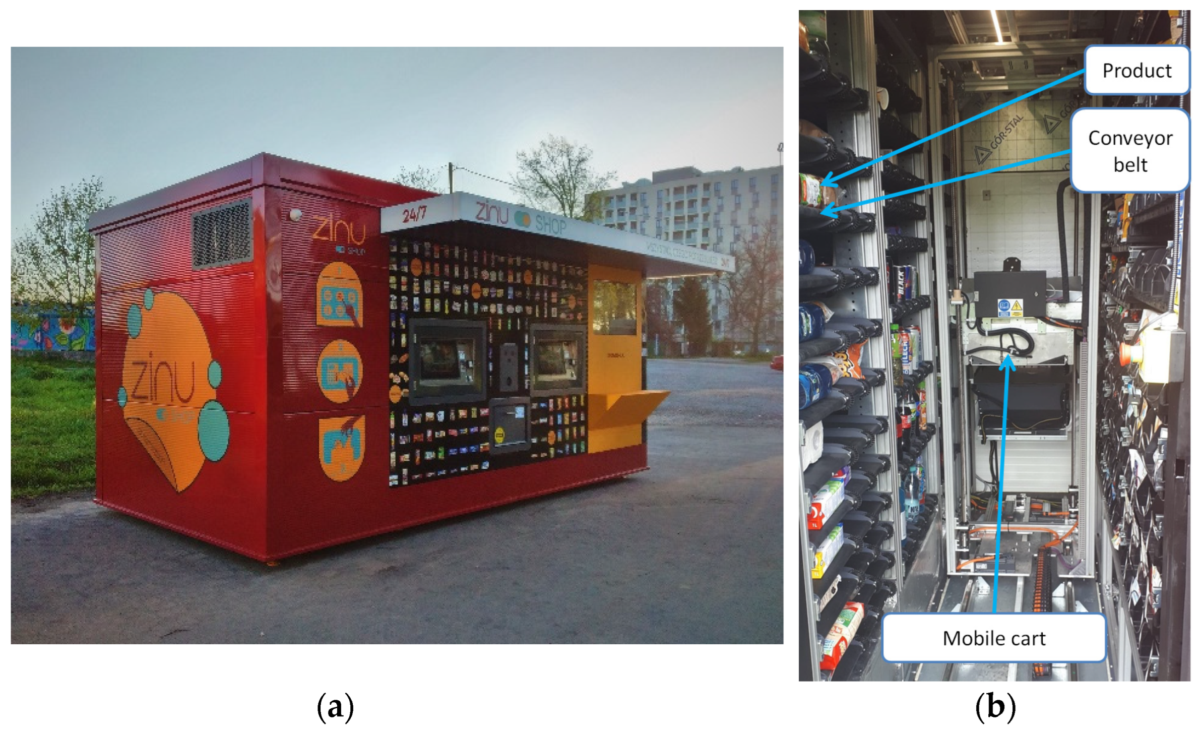
Delfin company from Nowa Wies, Poland, which deals with the design and construction of automated stores, performed a preliminary estimation of the annual energy consumption of an automated store and compared the obtained results to the energy consumption measured for a conventional store. The average annual electricity consumption evaluated for a grocery store of an area of 70 m² amounted to approximately 38.4 MWh, while for an automated store of an area of 9 m² and a comparable product range, the electricity consumption was approximately 10.1 MWh, i.e., 74% smaller.

However, it should be stressed that the amount of electrical energy consumed by an automated store depends on many factors, such as geographical location and changes in the climatic conditions, including the store’s external temperature. The external temperature of the store determines the amount of energy consumed by the heating, ventilation, and air conditioning (HVAC) or heating and air conditioning (HAC) units, which ensures the appropriate conditions for storing the products. Another important factor is the number of products purchased by users, which translates into the amount of energy supplied to the electrical drives of the feeding system, which is activated when a store’s customer completes their shopping list.

The estimated energy demand for the store is the information of key importance for the potential investors and the manufacturer of the automatic store. Therefore, the research presented in the paper concerns the development of the model for determining the electricity consumption, operating costs and CO₂ emission of the automated store designed and developed by Delfin company.

In the designed automated store, three basic systems responsible for the electrical energy consumption were distinguished: the feeding system, the HAC unit and other electrical energy consumption points (marked in the paper as “others”), e.g., the operator panel with the automation system, lighting, outdoor advertising screens, etc.

In many scientific works concerning the development of the energy consumption models, machine learning algorithms are used. The most commonly used algorithms are LSTM (long short-term memory) [7,8,9,10], MLP (multilayer perceptron) [11,12], MLR (multiple linear regression) [13,14], ANN (artificial neural network) [15,16,17,18,19], SVR (support vector regression) [20,21], BPNN (back propagation neural network) [22], SVM (support vector machine) [20,23], XGB (extreme gradient boosting) [24,25] and RF (random forest) [26,27]. Authors of these scientific papers often point out the possible fields of application of such solutions, e.g., controlling HVAC systems. Practical applications of ML algorithms involve the use of extensive databases, usually containing many types of measured values. As an example, [5] can be taken, in which the authors compared the MLR, JPR (joinpoint regression), BP (back propagation), RF and JP-MLR (joinpoint−multiple linear regression) models, for which they used eight variables for analysis: five continuous variables (average outdoor air temperature, average relative humidity, daily global radiation intensity, average wind speed and daily temperature amplitude) and three decisive variables (gender of inhabitants, holiday index and sunshine index during the day).

Another approach consists of the usage of thermal models of buildings. In this case, three methodologies are most frequently used [28,29]: the temperature response method, e.g., [30], the finite difference method, e.g., [31], and the lumped heat capacity method, e.g., [32]. The application of the lumped heat capacity method allows for the relatively easy determination of a mathematical model of temperature changes [28,29,33], while the physical parameters can be determined based on the parameters of materials used in the construction of the building of interest (such as the heat capacity or thermal resistance of the constructional elements) [28].

The novelty of the carried-out research results consists of the development of the first known energy consumption model for an automated store with a container structure. It should be stressed that the developed model provides results with sufficient accuracy, which has been validated experimentally for a single location.

In order to determine the automated store’s energy consumption, the temperature data from a nearby meteorological station were sufficient; over the course of the research, it has been proven that it does not have to be measured at the exact location of the store.

Forecasting the value of the automated store’s energy consumption in the various environmental conditions based on the data from the publicly available sources, such as meteorological stations, is convenient from a practical point of view. It enables quick access to a set of information concerning climatic conditions for a given location—the place where the store is installed. However, the information from meteorological stations, e.g., temperature, is often averaged for a given area, with a relatively low number of samples (low sampling frequency). Therefore, for the selected model, it was necessary to carry out the tests to determine the impact of the input data in the form of the measurements from the meteorological station on the accuracy of the calculations and, consequently, on the output values of the model.

In order to calculate the energy consumption of the store’s feeding system, it was necessary to solve the problem of finding a correlation between the energy consumption of the electrical drives of the feeding system and the arrangement of products on the store shelves, which are made up of belt feeders. Depending on the type and quantity of products selected by the customer, the movement trajectory of the feeding system is generated. The total permissible capacity of the goods that the manipulator can transport in one work cycle is limited by the volume of its container.

For a given customer’s shopping list, by knowing the approximate volume of each type of product, the store management system can optimize the length of manipulator trajectory necessary to complete the order. This is beneficial in terms of the order processing time and the amount of electrical energy necessary to power the engines during their operation. However, from the point of view of the created model, it results in the high complexity of the mathematical notation.

Additionally, the set of input parameters of such a model is a shopping list containing the exact number of products of different types, which is difficult to define at the stage of preliminary research regarding the interest of the consumer market. In the carried-out research, the general guidelines for the operation of the store model assumed the calculation of the average value of energy consumption per product, which ensured a simple analysis for various sale variants.

Project assumptions regarding the minimum number of types of data sets necessary to estimate the energy consumption, CO₂ emission and costs over the assumed average operating period of one month (approximately 30 days) resulted in the final choice of the model description for the HAC unit based on the lumped method heat capacity, and a linear relationship between the energy consumption coefficient per product for the feeding system.

2. Automated Store

The automated store developed by the company Delfin sp. z. o. o. (Nowa Wies, Poland) has the form of a container of dimensions of 3 × 3 × 6 m (height, length, and width), as shown in Figure 1a.

The device can hold approximately 350 different products, e.g., bread, vegetables, fruit, dairy products, fats, cold cuts, drinks, sweets, spices, chemicals and many others. To ensure the proper storage of food products in the store, the internal temperature of the climatic chamber (volume of 27 m³) should be maintained in the range of 4–7 °C.

2.1. System for Monitoring the Store Parameters

The proper operation of the store is provided by a supervising system operating in an online mode, as shown in Figure 2. The system is responsible for monitoring basic operational parameters, such as internal temperature for eight measurement points, external temperature, humidity inside the store, the activation of the heating and cooling unit, current and power intensity for three measurement points.

The measurement system is equipped with PT1000 temperature sensors connected to an EL3208 module (measuring range: −60–250 °C) [34]. The measurement of power and current intensity is carried out by an EL3403 module (measuring voltage range: 500 V AC; measuring current range: 5 A, AC, via measuring transformers at a 40:5 A ratio) [35], equipped with a 16-bit analogue-to-digital converter.

In practice, the monitoring system ensures the quick detection of faults or failures by analysing the operating store parameters, which reduces the store’s service downtime significantly. The monitored parameters are archived, which makes it possible to identify the conditions in which operating anomalies occurred. Apart from monitoring the above-mentioned store operating parameters, the system sends information about the current stock of products, which allows for the planning of the replenishment of product shortages. Moreover, the system enables the on-line observation, via a virtual panel, of the operation of the manipulator and feeders, which are elements of the executive system of the automated store.

2.2. Feeding System Design

The product feeding system used in the store consists of a PPP-type serial manipulator, called “mobile cart” in the feeding system, and a set of belt feeders on which the products are placed, as shown in Figure 2b. The system is controlled in the Cartesian reference system shown in Figure 3.

Five Beckhoff servo drives were used to build the system, which ensures the movement of the manipulator along each of the axes of the assumed reference system and belt feeders. The mode of system standard operation includes the following sequences: accessing the starting point (where a product is collected) by the manipulator, coupling the gears, initiating the belt conveyor and transporting the selected product to the manipulator’s mobile cart, the disengagement of the feeder mechanism, accessing the point of picking up the goods by the customer.

3. Model of Energy Consumption

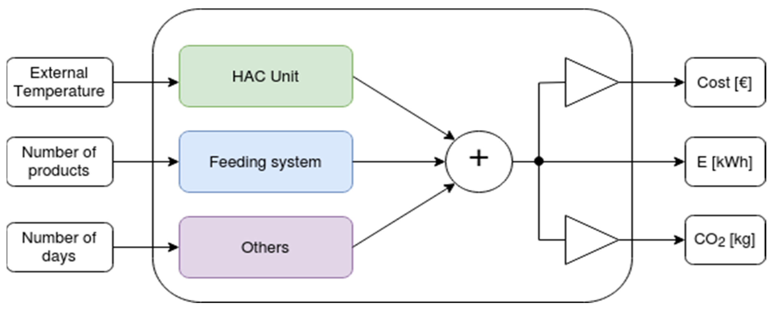
In the automated store model (Figure 4), the three main sources of energy consumption has been taken into account: HAC unit, feeding system and other electrical devices. The input data for the model are the outdoor temperature and the number of products sold. Based on the input data, the model calculates an estimated value of electricity consumption, the mass of CO₂ emitted as a result of generating this energy and the estimated cost of production.

The energy consumption of the considered automated store can be described as follows:

$$E_{Total}=E_{HAC}+E_{FE}+E_{OTH}$$

(1)

$$E=\int P_{HAC}\left(t\right)dt+\int P_{FE}\left(t\right)dt+\int P_{OTH}\left(t\right)dt$$

(2)

where E_Total—overall consumption of energy; E_HAC, E_FE, E_OTH—electrical energy consumed by the HAC unit, feeding system and other electronic components; P_HAC(t), P_FE(t), and P_OTH(t)—instantaneous power consumed by the HAC unit, feeding system and other electrical components, respectively.

3.1. Model of HAC Unit

The accurate modelling of the air temperature changes inside an automated store is not possible due to the complexity of the occurring physical phenomena. The temperature inside the store is influenced by a number of phenomena, including non-deterministic ones, such as: sunlight, ambient temperature, wind strength, number and type of products in the store assortment, frequency of purchases, frequency of deliveries, etc. Therefore, it is only feasible to develop the approximate mathematical models of temperature changes inside the store and electrical energy consumption. The equations on the basis of which the model proposed in this research has been developed are presented below.

$$P_{heat}=\frac{d{Q}_{heat}}{dt}=T_{heat}-T_{int}·M_{dot}·c_{air}$$

(3)

$$P_{cool}=\frac{d{Q}_{cool}}{dt}=T_{int}-T_{cool}·M_{dot}·c_{air}$$

(4)

$$P_{loss}=\frac{d{Q}_{loss}}{dt}=\frac{T_{out}-T_{int}}{R_{eq}}$$

(5)

$$\frac{d{T}_{int}}{dt}=\left\{\begin{array}{c}\frac{d{T}_{int}}{dt}=\frac{1}{M_{air}·c_{air}+M_{eq\_rest}·c_{eq\_rest}}·{(P}_{loss}+P_{eq\_eq}+P_{heat}),\hspace{1em}\hspace{1em}(forheating)\\ \frac{d{T}_{int}}{dt}=\frac{1}{M_{air}·c_{air}+M_{e{q}_{\_rest}}·c_{eq{\_}_{rest}}}·{(P}_{loss}+P_{e{q\_}_{eq}}-P_{cool}),\hspace{1em}\hspace{1em}(forcooling)\end{array}\right.$$

(6)

$$P_{HAC}\left(t\right)=P_{HAC\_Standby}\left(1-u_h\left(t\right)-u_c\left(t\right)\right)+P_{HA{C}_{Heat}}·u_h\left(t\right)+P_{HA{C}_{Cool}}·u_c\left(t\right)$$

(7)

$$u_h\left(t\right)+u_c\left(t\right)\le 1$$

(8)

where T_int, T_out—temperature inside and outside the store, respectively; T_heat, T_cool—temperatures of warm and cold air from the cooling and heating unit, respectively; M_air, M_{eq_rest}—mass of air inside the store and the equivalent mass of other elements (except air) present inside the store (including food products, equipment elements, feeders); M_dot—air mass supplied from the HAC unit per unit of time; c_air, c_{eq_rest}—heat capacity of air at the constant pressure and the equivalent heat capacity of other elements (apart from air) inside the store (including food products, equipment elements, feeders), respectively; P_heat, P_cool, P_loss—heating and cooling power of the HAC unit and the power loss, respectively; P_{eq_eq}—equivalent power emitted by elements inside the facility (including power supplies, electronic systems and electric drives); P_{HAC_Standby}, P_{HAC_Heat}, P_{HAC_Cool}, P_AC—electrical power consumed by the heating and cooling unit in the standby, heating and cooling states, and the overall electrical power consumed by the heating and cooling unit; u_h(t), u_c(t)—time histories of on/off signals for heating and cooling, respectively.

Equations (3) and (4) describe heat flow in the cooling and heating unit working in the heating and cooling modes, respectively. The parameter M_dot represents the mass of air injected by the HAC unit. It was estimated on the basis of the air density and flow provided in the HAC catalogue note and then corrected in a way that allows for the best tuning of the model to the real data. Equation (5) describes thermal power losses resulting from the usage of materials with the equivalent thermal resistance Req in the construction of the store. It was assumed that the equivalent thermal resistance is equal to the thermal resistance of the PUR (polyurethane) foam used for insulation, and its value was read from the manufacturer’s documentation. Equation (6) describes the variability of the temperature inside the store, taking into account the power supplied by the HAC unit, heat losses resulting from the finite thermal resistance of the structural elements and the equivalent power dissipated in the form of heat by the store equipment elements located inside, i.e., power supplies, electronic systems, electrical drives. The latter was estimated based on the measurements of electrical energy consumed by the store and the efficiency of individual components. In order to tune the model, it was also necessary to estimate the mass of air and the mass of other elements inside the store (mainly food products and equipment), as well as the equivalent heat capacity of these elements.

These values were initially estimated on the basis of the average amount of products available inside the automated store, and then adjusted to obtain the best fit of the model to the real object. Equations (7) and (8) make it possible to determine the electrical energy consumption based on the time histories, thereby determining the moments the thermostat was turned on and off by the heating and cooling unit.

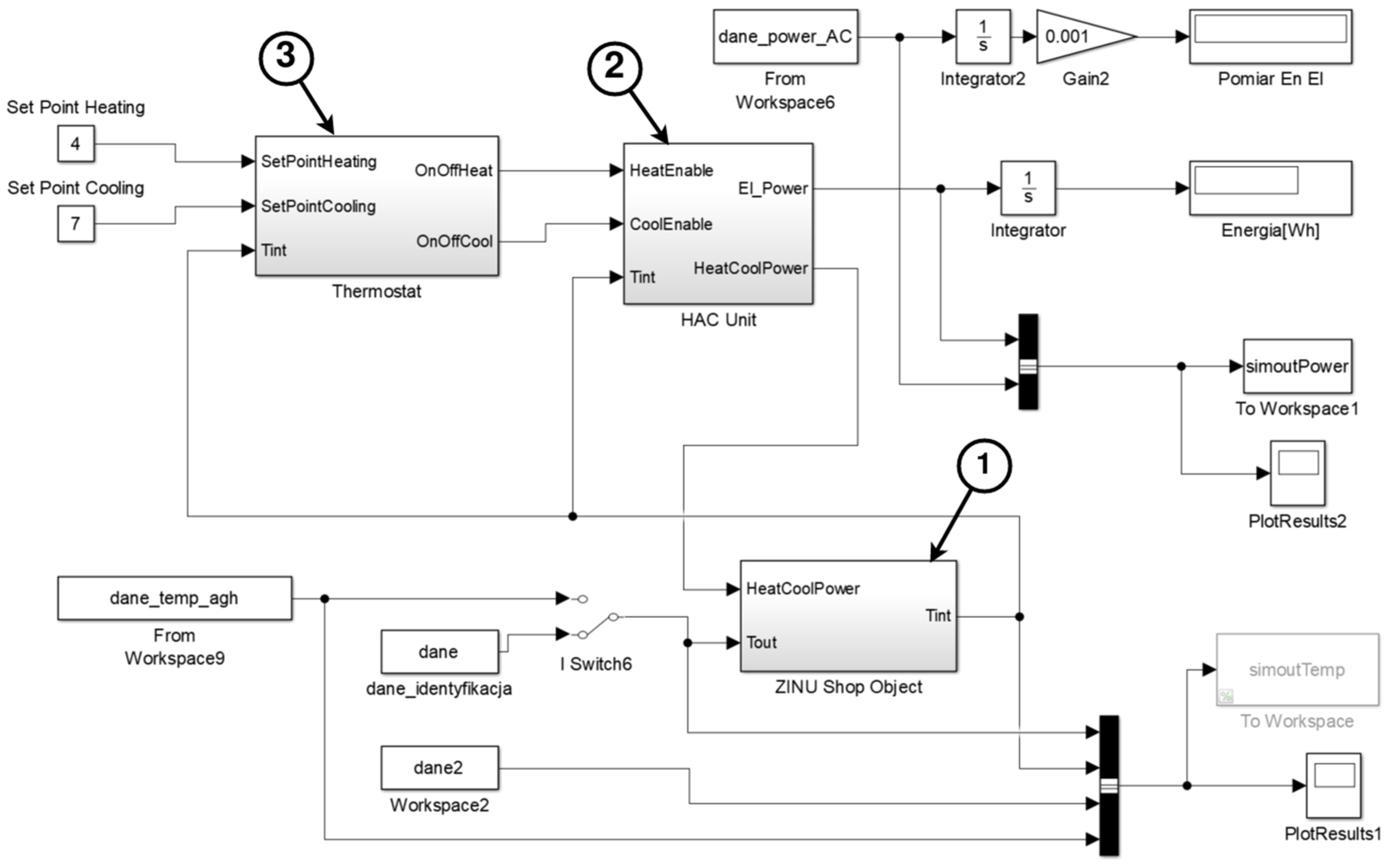
A diagram of the electrical energy consumption model developed in the MATLAB/Simulink environment is presented in Figure 5. The main elements of the developed model are blocks representing a thermostat, a cooling and heating (HAC) unit, and a store container.

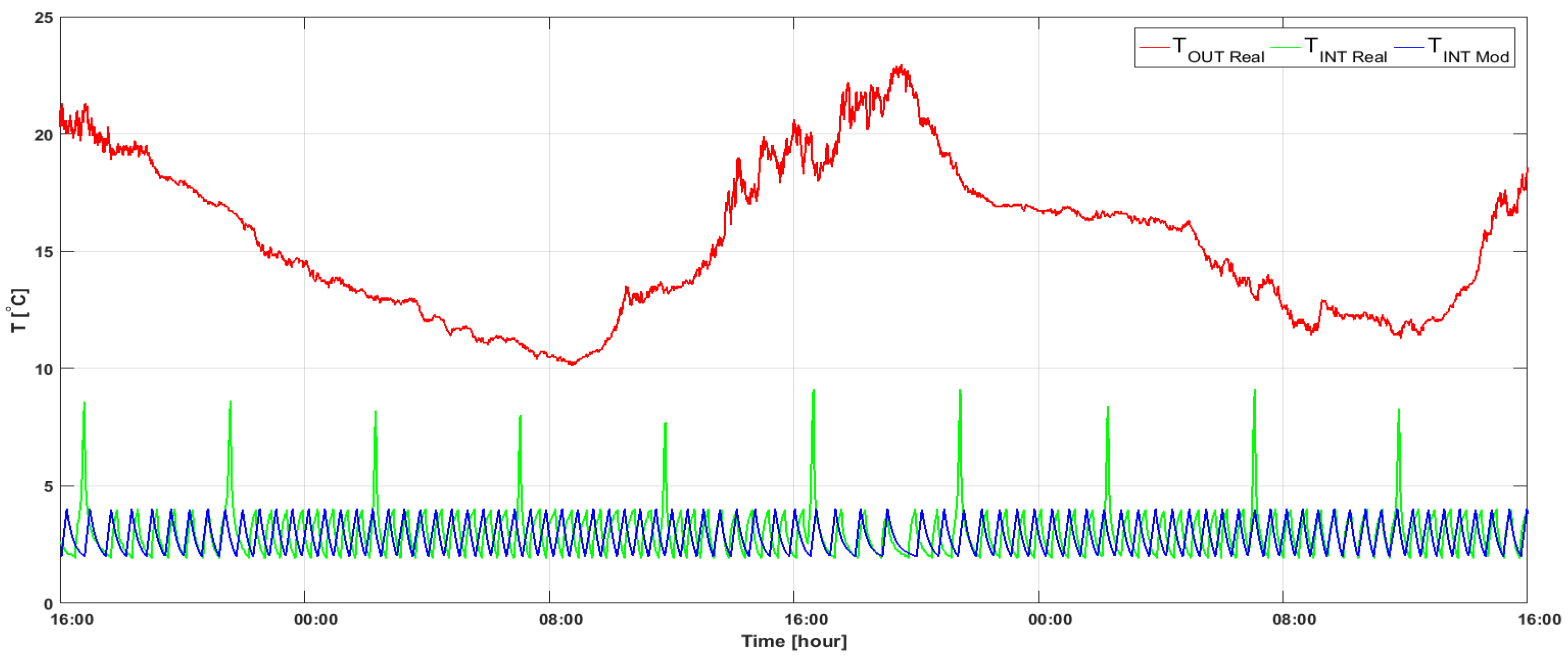
The first experiments on the HAC unit model concerned the identification of the model parameters. The model input includes a set of measured outdoor temperature values (Figure 6, T_{OUT Real}) obtained from the automated store monitoring system (Section 2.1).

The measurement time amounted to one day (24 h), and the sampling frequency was equal to 0.033 Hz. A comparison of the recorded temperature inside the store (Figure 6, T_{INT Real}) and the temperature obtained at the model output (Figure 6, T_{INT Mod}) allowed for the determination of the values of the model parameters, including the equivalent heat capacity (c_{eq_rest}, Equation (6), page 7) of objects inside the store (food products, equipment elements, manipulator and feeders).

Approximately 80% of the total capacity of the goods in the store consisted of liquids, which, in the model, was assumed as 40% of the store volume with the heat capacity of water. In the model, the equivalent power (P_{eq_eq}, Equation (6), page 7) generated by the elements inside the store (including power supplies, electronic systems and electric drives) was also determined.

The total electrical energy consumption of the store HAC unit for the measurement day amounted to 22.49 kWh, while for the model, it amounted to 23.10 kWh. The absolute error was equal to 0.61 kWh.

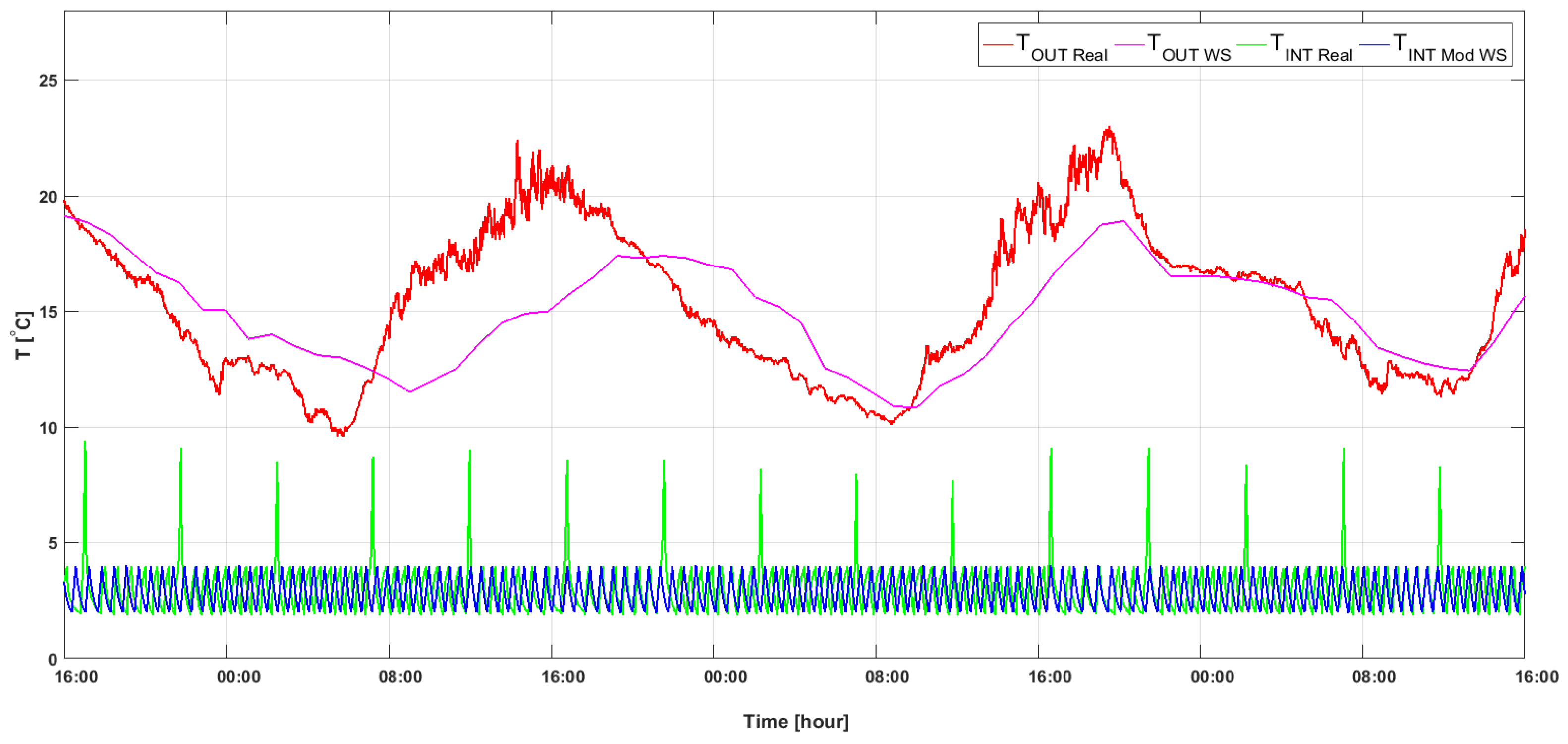
The third test that was carried out over the course of the research concerned/aimed at investigation on the model for a set of external temperature values obtained from the meteorological station [36] for the Krakow region, southern Poland. The data set covered a measurement period of 72 h, and the sampling period was 60 min. The outside temperature varied from 12 to 19 °C.

In Figure 7, time histories of the external (T_{OUT Real}) and internal (T_{IN Real}) temperatures registered by the store measurement system, external temperature T_{OUT WS} registered by the meteorological station, and the temperature inside the store T_{IN MOD WS} estimated from the model are presented.

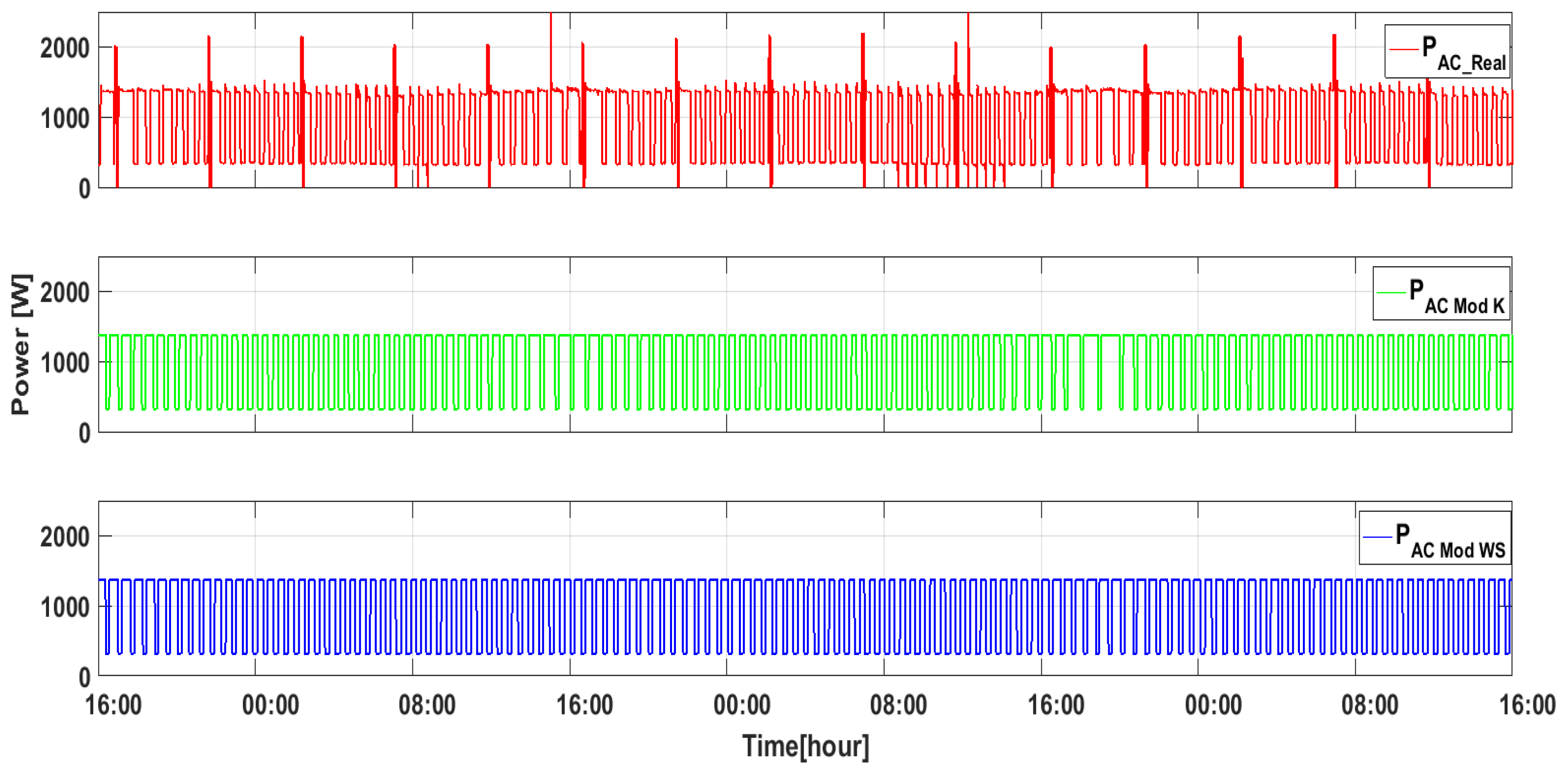
The last step of model validation consisted of a comparison of the measured and estimated energy consumption of the HAC unit. A comparison of time histories of the HAC unit’s electrical power, measured (P_{AC_Real}) and estimated for the assumed model (P_{AC Mod K}), is presented in Figure 8.

The values of total energy consumption of the store (E_{AC Real}) and the total energy consumption (E_{AC Mod R} and E_{AC Mod WB}) calculated by the HAC model for two sets of external temperatures (T_{OUT Real}, T_{OUT WS}) are listed in

Table 1. Total electrical energy consumption for a measurement time of 72 h.

EAC Real (kWh)	EAC Mod K (kWh)	EAC Mod WS (kWh)
67.63	69.27	68.12

. Obtained results made it possible to calculate the absolute error (AE) and the percentage absolute error (APE). For the energy consumption E_{AC Mod R}, these errors amounted to 1.64 kWh (2.4%), while for E_{ACMod WB}, it amounted to 0.49 kWh (0.7%).

The proposed model was also tested in the conditions of switching on the HAC unit heating mode. In order to verify the model correctness, the measurements gathered during 3 consecutive days (from 10 January to 12 January 2021) were used. The recorded external (outdoor) temperature varied in the range from 12 °C to −8 °C, and the average value was approximately 1 °C.

Analogously to the previously considered case, the errors for the HAC unit energy consumption calculated from the model did not exceed 2% for the external temperature measured by the store measurement system nor 1% for the external temperature recorded by the meteorological stations.

3.2. Model of Feeding System

In the first developed model of energy consumption by the store’s feeding system, on the basis of carried-out experiments, a linear energy consumption coefficient per product was determined.

$$P_{FMod0}=f_{pp}\ast n_{op}$$

(9)

where:

• P_{F Mod0}—electrical power consumed by the elements of the feeding system;
• f_pp—coefficient of power consumption per product;
• n_op—number of products.

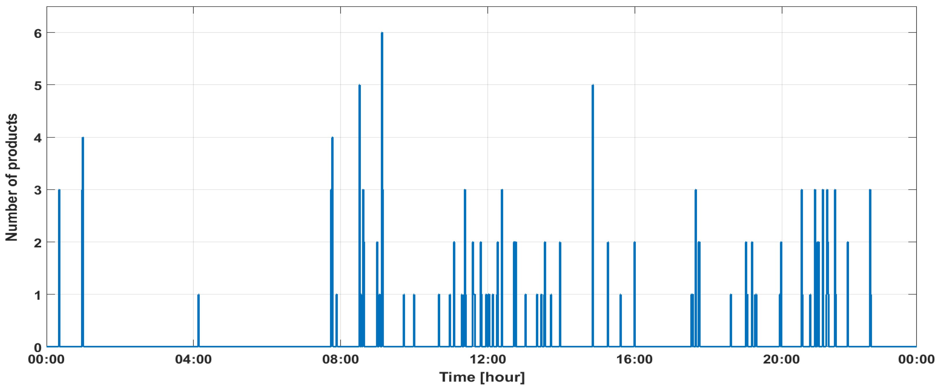
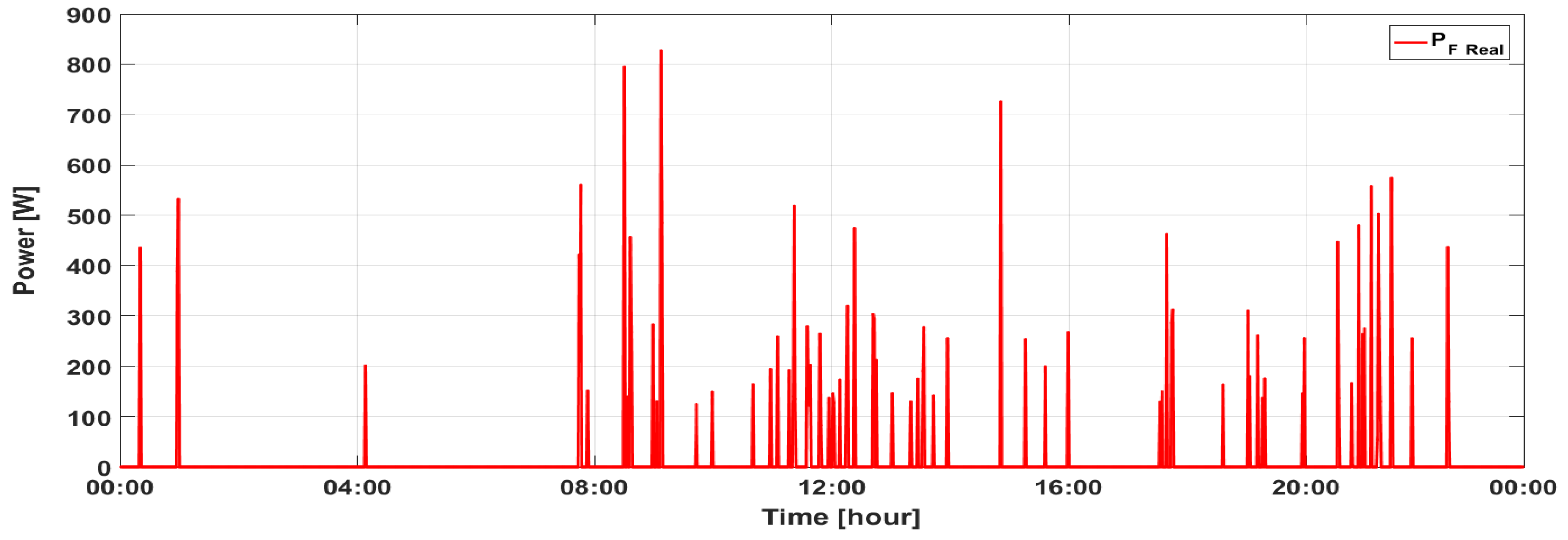
Over the course of the carried-out test, the first model was denoted by Mod 0. The value of the energy consumption coefficient per product was determined on the basis of measurements of the number of products (Figure 9) and power (Figure 10) carried out by the store’s monitoring system in a 24 h period. In total, 151 products were collected.

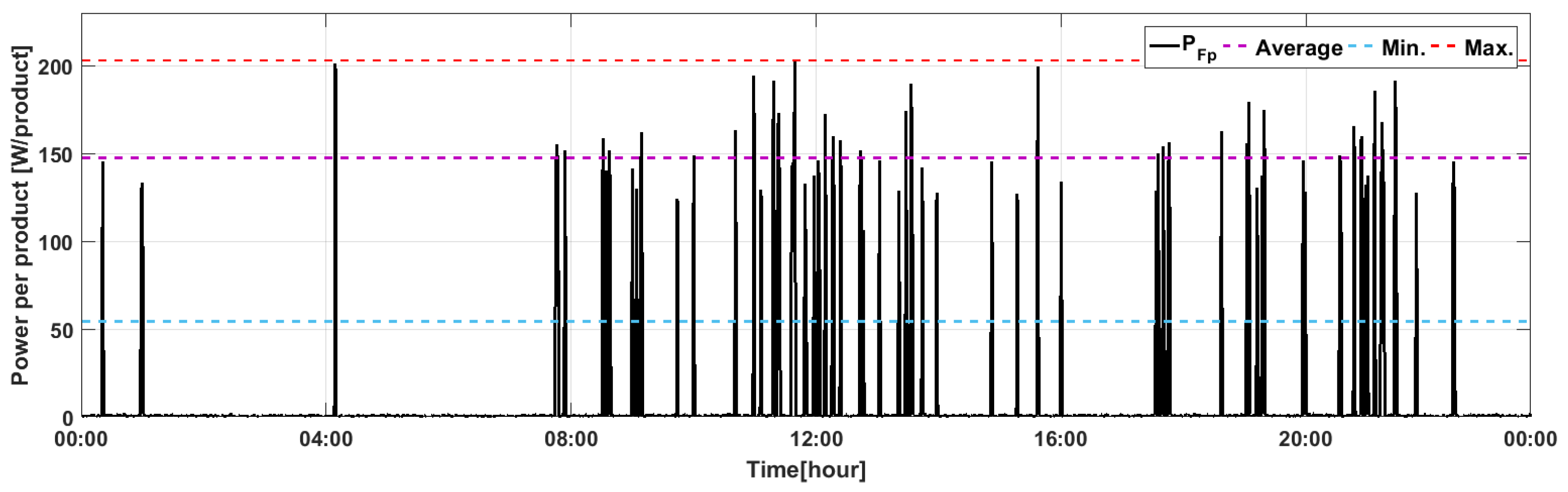
The results of the conducted experiment are presented in Figure 11. The maximum value of energy consumption per product (Figure 11, marked as Max.) amounted to 202.91 W/product, while the minimum value was 54.31 W/product. The obtained average value of energy consumption per product (Figure 11, Average) was equal to 147.47 W/product, and in further research, it will be used as the energy consumption coefficient per product ((9), f_pp).

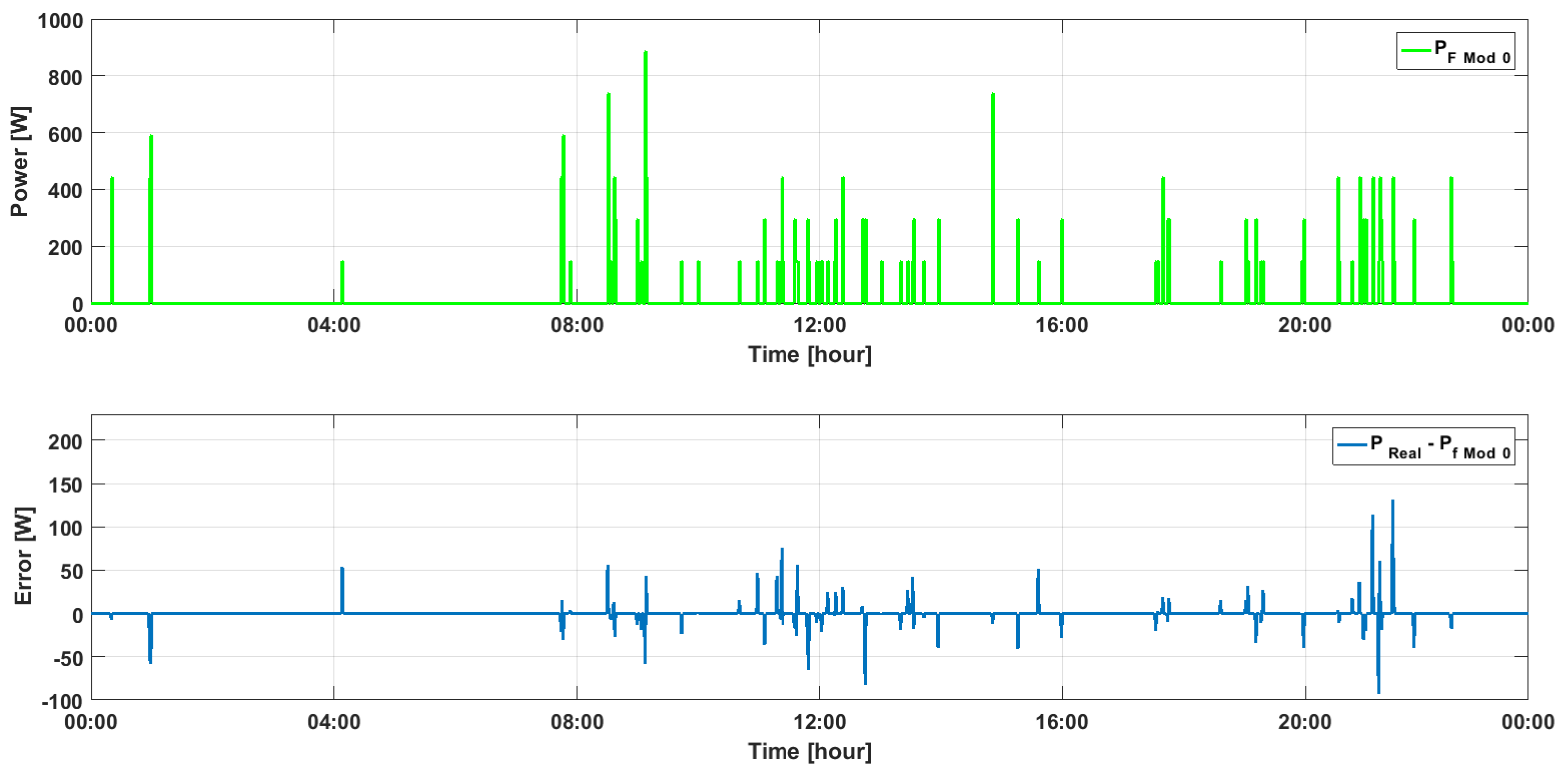
For the obtained energy consumption coefficient per product, a preliminary test was performed, which made it possible to determine the error between the measured value of power P_{F Real} (Figure 10) and the power value P_{F MOD 0} (Figure 12) estimated from the model.

In the case of three products being purchased, the maximum error regarding power estimation was 131.1 (W). For the considered experiment, which was carried out for a period of 24 h, the total energy consumption of the feeding system amounted to 0.372 kWh, while the value calculated by the model was 0.371 kWh, and thus, the absolute percentage error (APE) was equal to 0.3%.

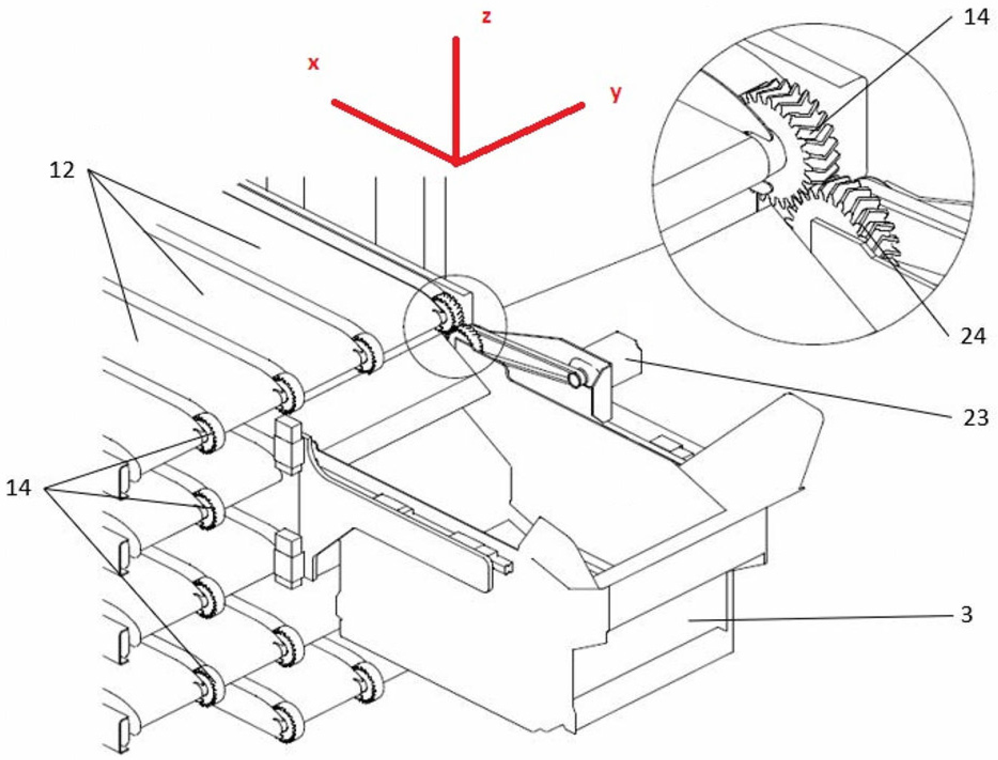
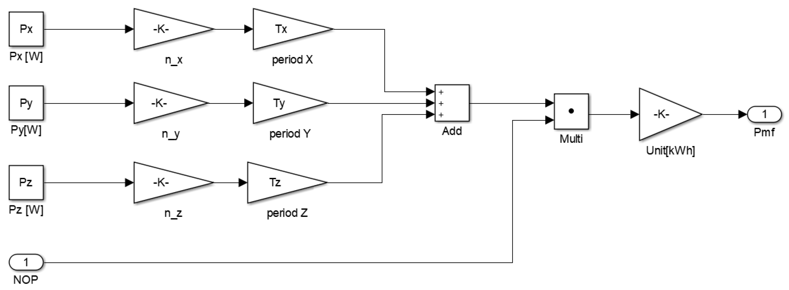
The second proposed model of energy consumption of the store’s feeding system was described by Equation (10) and denoted by Mod 1. Based on the orientation of the global coordinate system (Figure 3), the following notation was assumed (10):

$$P_{FMod1}=\left(P_x\times n_x\times {\Delta t}_x+P_y\times n_y\times {\Delta t}_y+P_z\times n_z\times {\Delta t}_z\right)\ast n_{op}$$

(10)

where n_x, n_y, n_z—number of drives in individual axes; P_x, P_y, P_z—the nominal power of the drives; Δt_x, Δt_y, Δt_z—drives activation time; n_op—number of products.

The average activation times of the drives in individual axes (Δt_x, Δt_y and Δt_z) were determined experimentally. For this purpose the following drive controllers were used: EL7211-9014 for AM8112 drives and AX8206 for AM8023 drives manufactured by Beckhoff.

These systems allow for the recording of the position, speed and acceleration, taking into account mechanical transmission ratios, with a maximum sampling frequency of 16 kHz, and the measuring of the motor current with a maximum sampling frequency of 32 kHz. The carried-out experiments aimed at determining the average activation (operation) time of drives in the consecutive axes, which is necessary to download the consecutive products form the store. The obtained experimental results are presented in the third column of

Table 2. Selected parameters of the store feeding system.

Axis	No. of Motors n	Activation Time (h) t	Rated Power (kW) P	Model of Motor Driver
x	1	0.000611	0.17	AM8112
y	2	0.000861	0.84	AM8023
z	2	0.000528	0.84	AM8023

. The scheme of the considered model implemented in the MATLAB/Simulink R2016a environment is presented in Figure 13.

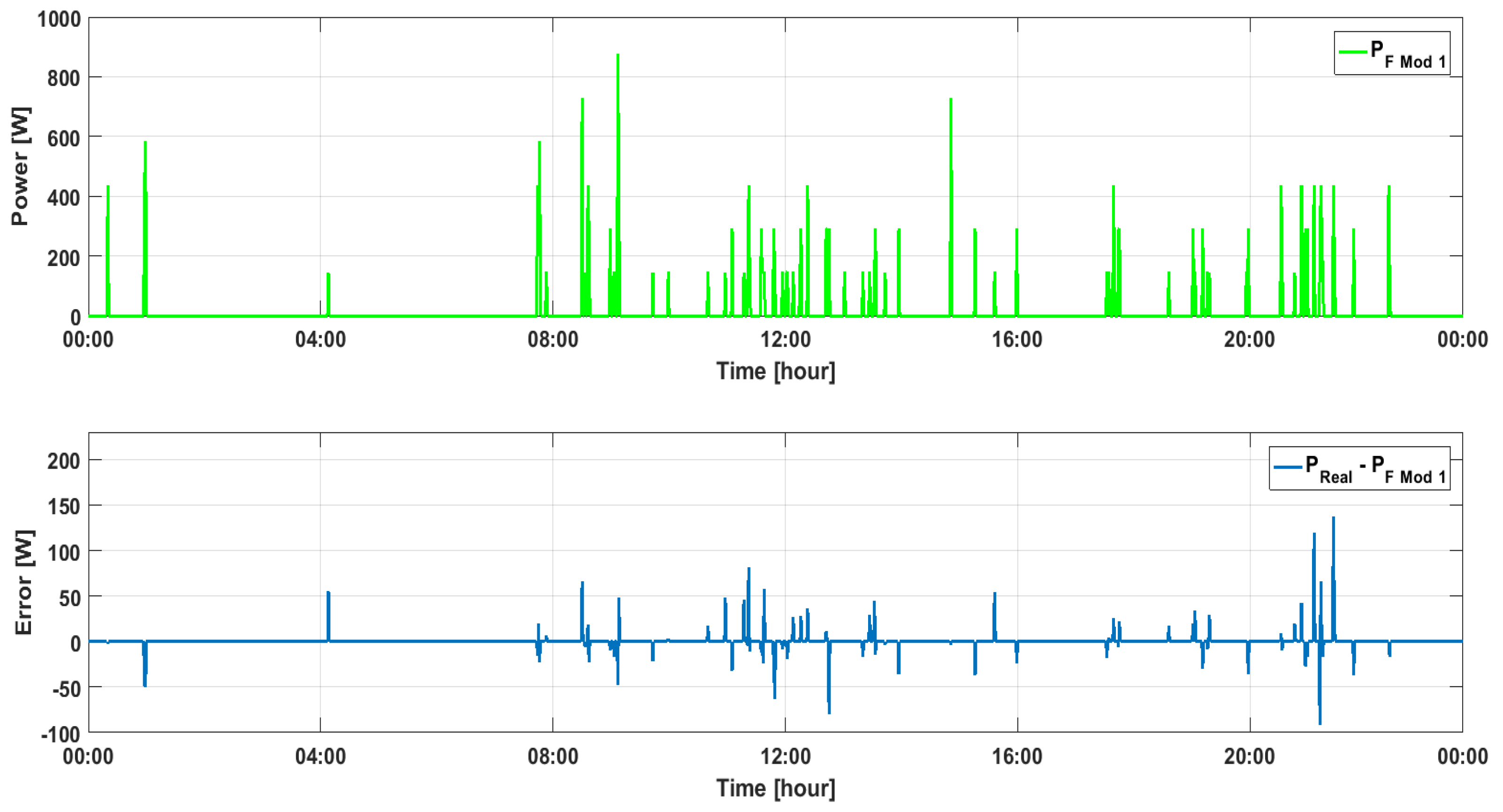
The difference between the measured power and power calculated from the model is presented in Figure 14. The maximal value of error, for three products downloaded, amounted to 136.5 W.

In the experiment carried out for a period of 24 h, the total energy consumption for the store’s feeding system amounted to 0.372 kWh, while the result obtained from the model amounted to 0.367 kWh. Therefore, the error of total energy consumption calculated for the store’s feeding system was equal to 5 W (1.4%).

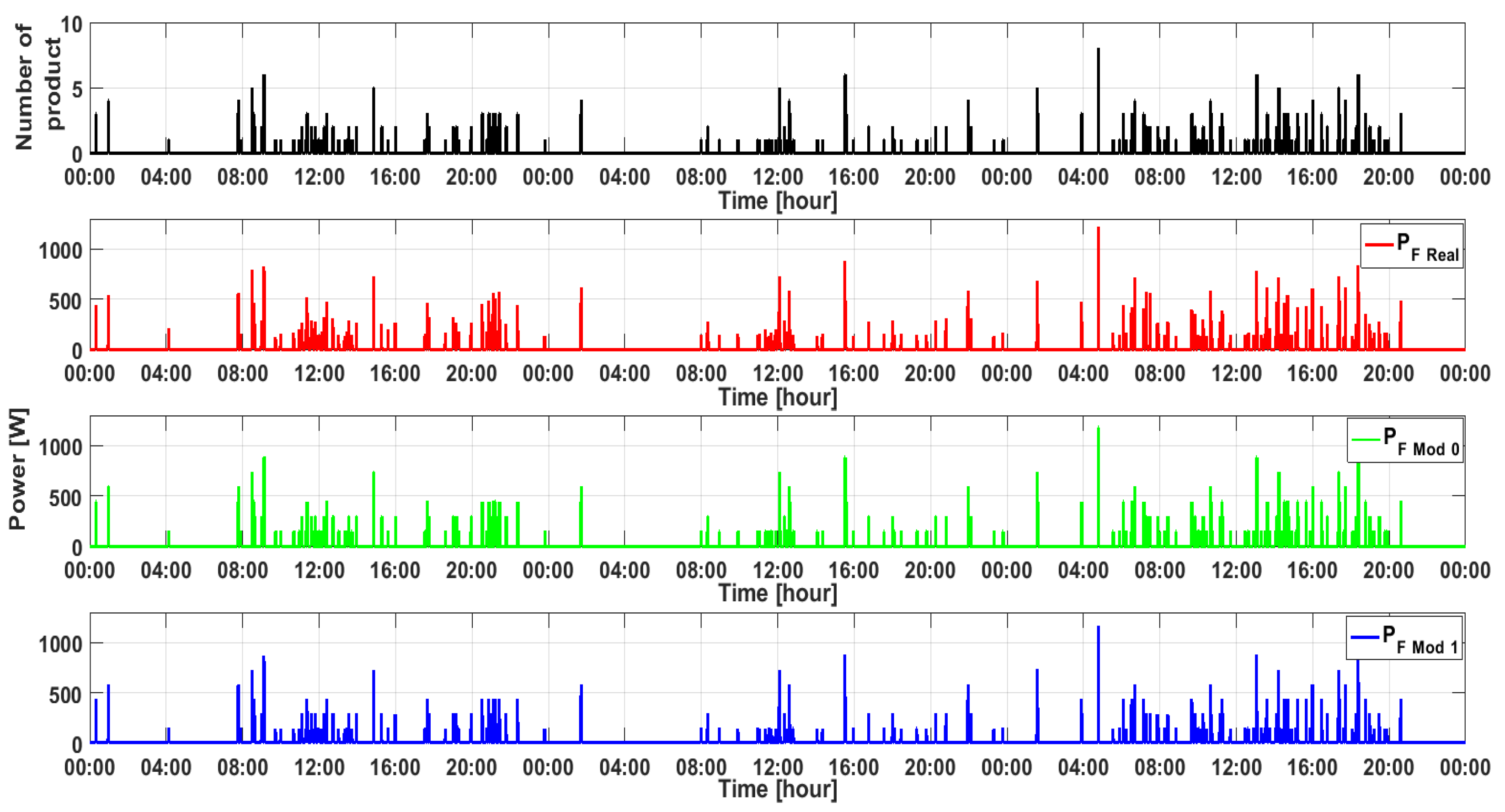
In the next test, the values of energy consumption per product were calculated for a time period of 72 h. The distribution of the number of products downloaded from the store is shown in Figure 15. The total number of products was 426.

In Figure 15, the results of the power measurements carried out for the considered system, P_Real, power computed by the model, P_{F Mod 0}, described by Equation (9) and power calculated by the model P_{F Mod 1} are presented and are described by Equation (10).

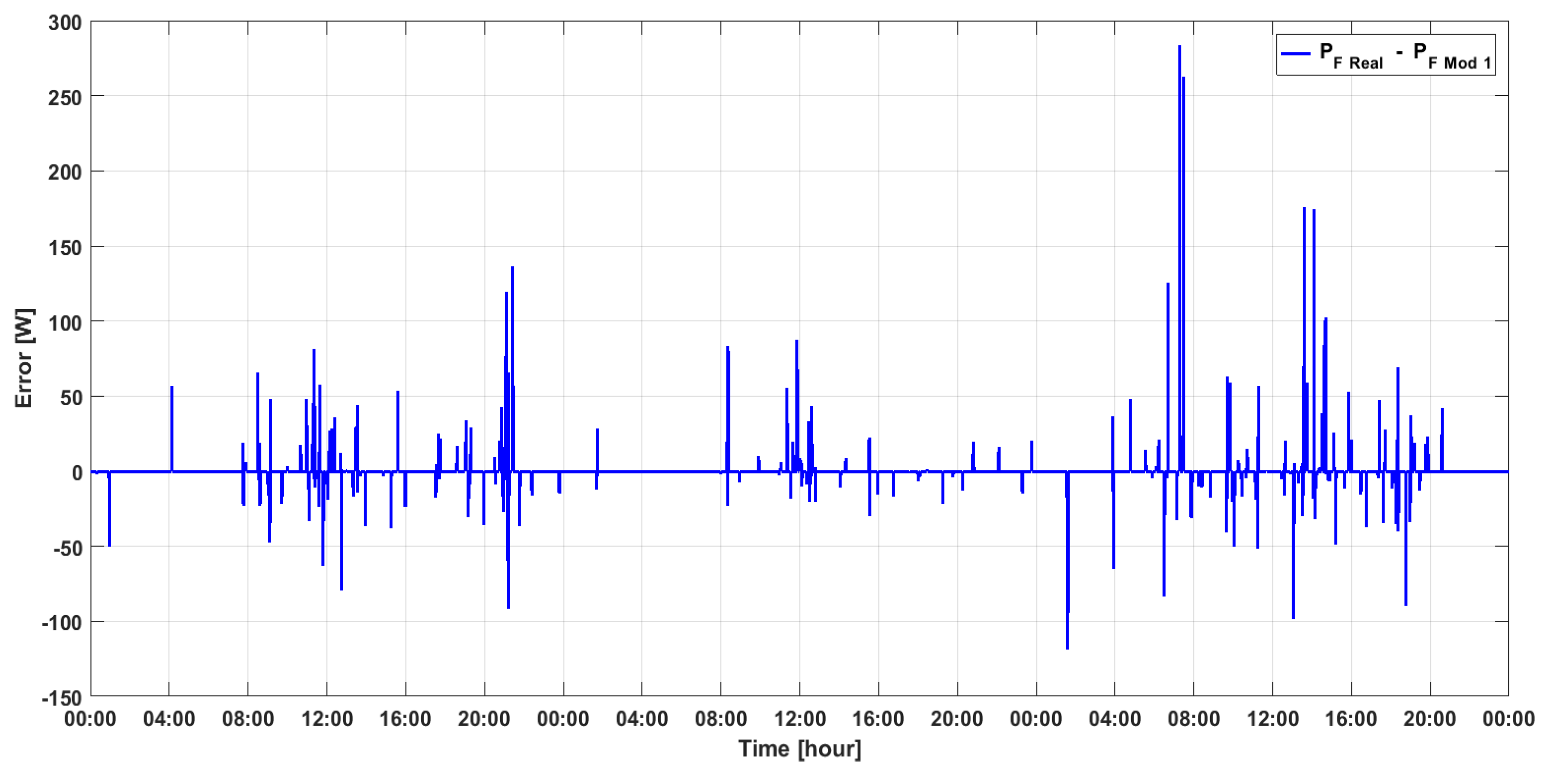
The difference between the power measured from the real object and power calculated by the second version model is presented in Figure 16. The maximal error value for a time period of 72 h was equal to 279.7 W for the first version of the model (Mod 0) and 283.3 W for the second version of the model (Figure 16).

For the purposes of comparing the results obtained from the models, the following error measures values were used: mean absolute error—MAE (11), mean absolute percentage error—MAPE (12), and mean squared error—RMSE—and the variability coefficient—CV (14).

$$MAE=\frac{1}{n}\sum _i^n\left|y_{real,i}-y_{mod,i}\right|$$

(11)

$$MAPE[\%]=\frac{1}{n}\sum _i^n\left|\frac{y_{real,i}-y_{mod,i}}{y_{real,i}}\right|\times 100\%$$

(12)

$$RMSE=\sqrt{\frac{{\sum }_i^n{\left(y_{real,i}-y_{mod,i}\right)}^2}{n}}$$

(13)

$$CV[\%]=\frac{RMSE}{\overline{y_{real}}}$$

(14)

where y_mod—sample calculated by the model; y_real—measured sample; n—total number of samples; $\overline{y_{real}}$—average value of all measured samples.

In order to calculate the factors affecting data, the real object power measurement data P_{AC Real} was used. The P_{AC Real}, which constitutes a set of samples (y_real), was compared to both the power data sets P_{F Mod 0} obtained for the first model and P_{F Mod 1} calculated by the second model. The samples of the data sets P_{F Mod 0} and P_{F Mod 1} were denoted by y_mod. The total number of samples n corresponded to the number of products taken from the store. The obtained results are presented in

Table 3. Values of errors MAE and MAPE for two versions of the feeding system model.

MAEF Mod 0 (W/pr)	MAEF Mod 1 (W/pr)	MAPEF Mod 0 (%)	MAPEF Mod 1 (%)
16.37	16.06	9.01	8.81

and

Table 4. Summary of the RMSE and CV errors for two versions of the store’s feeding system models.

RMSEF Mod 0 (W/pr)	RMSEF Mod 1 (W/pr)	CVF Mod 0 (%)	CVF Mod 1 (%)
34.86	35.03	23.43	23.55

.

The total energy consumption for the real object and models is presented in

Table 5. Total energy consumption determined for the feeding system for the 72 h measurements.

EF Real (kWh)	EF Mod 0 (kWh)	EF Mod 1 (kWh)
63.36	62.82	62.05

. The error of total energy consumption for the first version model (Mod 0) was equal to 0.54 kWh (0.9%), and for the second version model (Mod 1), it was 1.31 kWh (2%).

In the subsequent tests, it was decided that the second version of the model, Mod 1, was to be used. The justification for the choice is presented in Section 5.

4. Validation of Models

Further tests concerned the calculation of total energy consumption in the automated store for a measurement period of 4 months, from January to April 2023. The obtained results, including total energy consumption, considered both individual months and the entire measurement period. The formulated model takes into account the value of constant energy consumption, marked as “others” in Figure 4.

The tests were complemented by additional calculations, allowing for the analysis of the influence of changing the model input data set and the external temperature on the result of the electrical energy consumption by the HAC unit. Two temperature data sets were used: one from the store measurement system and the other from the online database of the meteorological station [36].

4.1. Results Tests of HAC Unit

The automated store measurement system archives the values of the measured external temperature every minute, while the data downloaded from the meteorological station server contains data are recorded every hour. For a greater transparency of the data presented, it was decided that the average values were to be calculated every day. Figure 17 presents changes in the average external temperature per day—T_avarage—calculated on the basis of the measurement data from the ZINU automated store and the data from the meteorological station—AGH Weather Station—over a period of four months. The value of the maximum daily temperature—T_max—and the minimum daily temperature—T_min—are also marked (Figure 17).

Temperatures T_c and T_h, as shown in Figure 17, determine the upper and lower limits of the required temperature inside the store—the climatic chamber. Their values constitute the parameters of the HAC unit thermostat settings. During the tests, these temperatures were equal to 7 °C and 4 °C, respectively.

For a period of four months, the maximum daily temperature recorded by the store measurement system was 30.12 °C on 24 April, and the minimum was −7.19 °C on 7 February. According to the data received from the AGH Weather Station, the highest value of the daily temperature was 23.6 °C on 29 April, and the lowest was −10.24 °C on February 7.

Over the course of the tests, the daily energy consumption of the HAC unit was calculated for a time period of four months. The obtained results are presented in Figure 18.

The obtained results of daily energy consumption for the HAC unit were used to calculate the absolute error (Figure 19) between the measured value—E_Real and values calculated by the model for two sets of input data—E_{HAC Mod WS} and E_{HAC Mod K}.

To compare the results obtained from the model, the following error measures were calculated: mean absolute error—MAE (11), mean absolute percentage error—MAPE (12), root mean square error—RMSE and coefficient of variation—CV (14). For the calculation of the error measures the measurement of real daily energy consumption—E_{HAC Real} was used, which was compared to the energy consumption calculated by the model: E_{HAC Mod K} and E_{HAC Mod WS} for the temperature measured by the store measurement system and the temperature from the meteorological station, respectively. The results are presented in

Table 6. MAE and MAPE error measures calculated on the basis of daily energy consumption for the HAC unit.

Month	MAEHAC Mod K (kWh)	MAEHAC Mod WB (kWh)	MAPEHAC Mod K (%)	MAPEHAC Mod WS (%)
January	2.5	2.34	15.65	14.62
February	1.37	1.69	6.76	8.23
March	1.7	3	7.23	12.84
April	2.37	4.48	9.98	22.27
January–April	2	2.89	9.98	14.62

and

Table 7. Summary of RMSE and CV measures calculated based on daily energy consumption for the HAC unit.

Month	RMSEHAC Mod K (kWh)	RMSEHAC Mod WS (kWh)	CVHAC Mod K (%)	CVHAC Mod WS (%)
January	2.78	2.73	16.53	16.28
February	1.75	2.23	8.82	11.22
March	2.19	3.55	9.3	15.05
April	2.98	5.31	12.14	21.66
January–April	2.49	3.56	11.72	17.27

.

Table 8. Total energy consumption of the HAC unit.

Month	ETotal HAC Real (kWh)	ETotal HAC Mod K (kWh)	ETotal HAC Mod WS (kWh)
January	521.59	599.33	590.40
February	575.76	556.61	538.34
March	731.33	726.29	664.64
April	736.23	746.01	676.14
January–April	2564.91	2628.24	2469.52

presents the HAC unit total energy consumption determined for individual months and for the entire measurement period, where: E_{Total HAC Real}—the total energy consumption calculated on the basis of the measurements at the real store, E_{Total HAC Mod K}—the total energy consumption calculated by the model based on the temperature measured at the real store, E_{Total HAC Mod WB}—the total energy consumption calculated by the model based on data from the meteorological station.

Based on the data from Table 8, the value of the absolute error—AE and the absolute percentage error—APE were calculated (

Table 9. Values of AE and AP errors, calculated on the basis of the total energy consumption of the HAC unit.

Month	ErrorHAC Mod K (kWh)	ErrorHAC Mod WB (kWh)	APEHAC Mod K (%)	APEHAC Mod WS (%)
January	−77.74	−68.81	15	11.5
February	19.15	37.42	3	6.7
March	5.04	66.69	0.7	9.2
April	−9.78	60.09	1.3	8.1
January–April	−63.33	95.39	2.5	3.6

).

4.2. Results Test of Feeding System

The second version of the model described by Equation (10) was used for testing the automated store feeding system performance over a period of four months. Based on the number of products sold in each month, the total energy consumption was calculated.

The results are presented in

Table 10. Total energy consumption of the store feeding system.

Month	Nr. of Products	EF Real (kWh)	EF Mod (kWh)
January	3209	7.80	7.79
February	2882	6.94	7.00
March	3285	8.27	7.98
April	3146	7.30	7.64
January–April	12,522	30.31	30.40

, where: E_{F Real}—the total energy consumption measured for the feeding system, E_{F Mod}—the total energy consumption of the feeding system calculated by the model.

Based on the obtained values of total energy consumption, the error and the absolute percentage error APE were calculated (

Table 11. Error and APE calculated on the basis of the total energy consumption of the store feeding system.

Month	ErrorF Mod (kWh)	APEF Mod (%)
January	0.01	0.1
February	−0.06	0.9
March	0.30	3.6
April	−0.34	4.7
January–April	−0.09	0.1

).

4.3. Complete Model

In the assumed model of the automated store energy consumption, apart from the HAC unit and the store feeding system, the power consumption of other devices—electrical systems called “others”, was taken into account (Figure 4).

Based on the measured average electrical energy consumption, which amounted to 13.5 kWh per day, the monthly energy consumption value and energy consumption for the entire measurement period were calculated (

Table 12. Total energy consumption of the store remaining electrical appliances (the “others”).

Month	EOther (kWh)
January (31 *)	418.5
February (28 *)	378
March (31 *)	418.5
April (30) *	405
January–April (120 *)	1620

* number of days in a month and the last row months.

).

Based on the Formula (1), the total energy consumption for the automated store was calculated for the measurement period of four months. The results are presented in

Table 13. Automated store total energy consumption.

Month	ETotal Real (kWh)	ETotal Mod K (kWh)	ETotal Mod WS (kWh)
January	995.36	1025.62	1016.69
February	958.87	941.61	923.34
March	1156.9	1152.77	1091.12
April	1099.5	1158.65	1088.78
January–April	4210.63	4278.641	4119.921

, where: E_{Total Real}—measured total energy consumption, E_{Total Mod K}—calculated total energy consumption taking into account the HAC unit model for the measured temperature, E_{Total Mod WS}—calculated total energy consumption taking into account the HAC unit model for the temperature read from the meteorological station.

In order to compare the obtained results in the form of the automated store total energy consumption over a period of four months, the values of AE and APE errors were calculated (

Table 14. AE and APE errors calculated on the basis of the automated store total energy consumption.

Month	AETotal Mod K (kWh)	AETotal Mod WS (kWh)	APETotal Mod K (%)	APETotal Mod WS (%)
January	30.26	21.33	3.04	2.14
February	17.26	35.53	1.80	3.71
March	4.13	65.78	0.36	5.69
April	59.15	10.72	5.38	0.98
January–April	68.01	90.71	1.62	2.15

).

The proposed model (Figure 4), based on the forecast energy consumption, calculates also the following values: the mass of CO₂ necessary to produce the required electrical energy and the energy cost. In

Table 15. CO₂ emission and energy production costs for the considered automated store.

Month	CO2 Emission (kg) 1	Energy Cost (EUR) 2
January	754	149
February	685	135
March	810	160
April	808	159
January–April	3057	603

¹ On the basis of the average CO₂ emission for Poland [37]: 742 [g/kWh]—average value for 12 months, current status for May 2022. ² Based on the average electricity price for Poland [38]: 0.1464 [EUR/kWh] average value for 12 months, current status for May 2022.

, the results of the remaining values are presented for the model, the total energy consumption of which was marked as E_{Total Mod WS} in Table 15.

5. Discussion

The first tests that were carried out over the course of the research presented in this paper allowed for the identification of the parameters of the thermal model of the automated store, including the equipment, assortment as well as the HAC unit. Both external temperature measurement data at the ZINU Shop location (recorded by the store’s measurement system) and generalized data for the given region obtained from a meteorological station were used as input data for the model.

The error of the HAC unit’s electrical energy consumption estimated from the data recorded over a three-day period with respect to the results obtained from the developed model (calculated on the basis of the input data in the form of the external temperature of the store) amounted to approximately 2.4%. However, for the outdoor temperature data obtained from a publicly accessible meteorological station, the error amounted to approximately 0.72%. The difference in the values of the above errors results from the different external-temperature time histories used as the model input.

One of the project assumptions concerned calculating the energy consumption of electrical drives per product. Two linear models were proposed: Equation (9), P_{F MOD 0}; and Equation (10), P_{F MOD 1}. The first one was based on the power factor per product determined experimentally. The second model took into account the actuation times of the drives, their number and rated power (10). The results of preliminary tests for three measurement days allowed for a comparison of the models. The values of calculated errors and error measures, presented in Table 3 and Table 4, showed similar values of deviation in power consumption per product. Taking into account that the motor parameters in the model make it possible to easily introduce the changes without the need to perform further experiments, it is possible to replace the drive in the feeding system with a drive of a different nominal power value since it does not affect the activation time. Therefore, for the further tests, the second model described by formula (10) was selected.

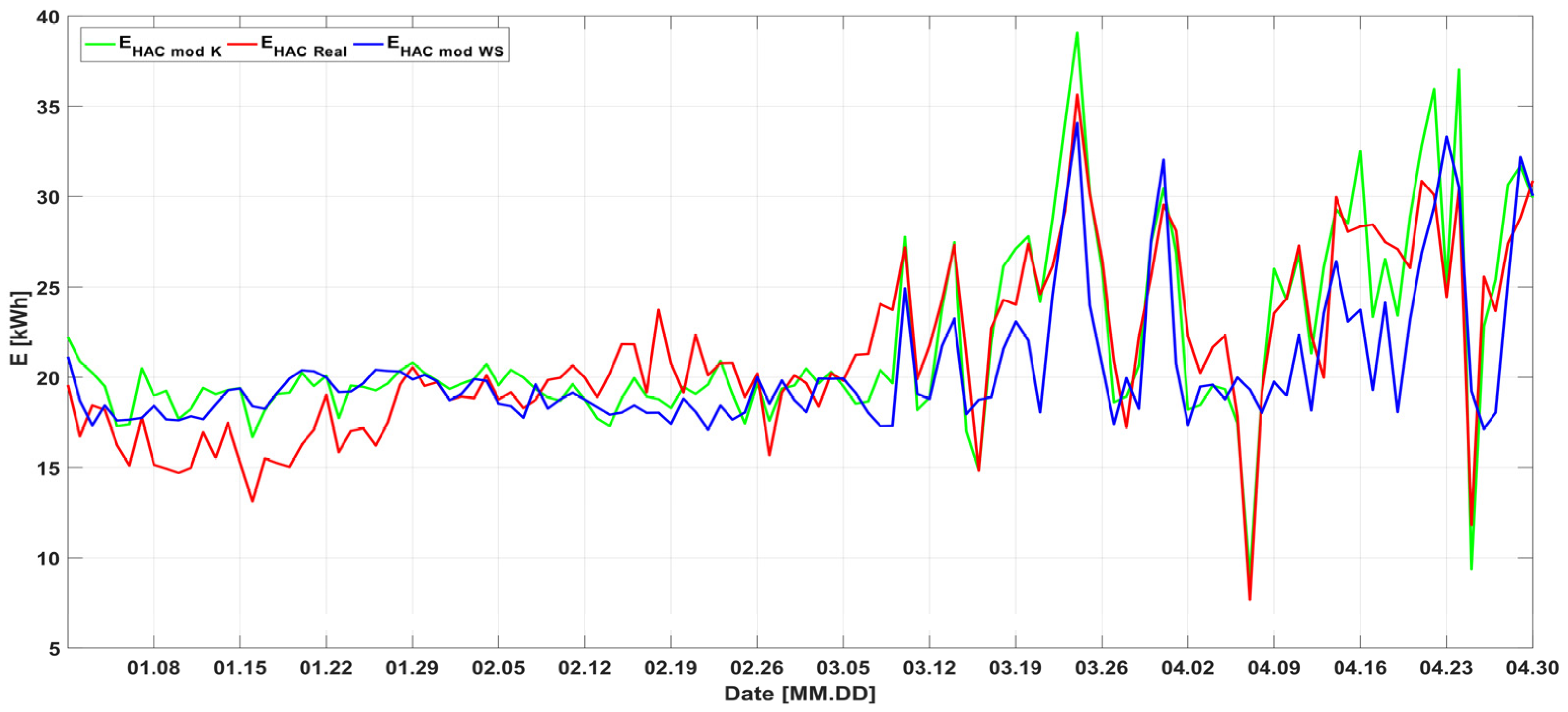
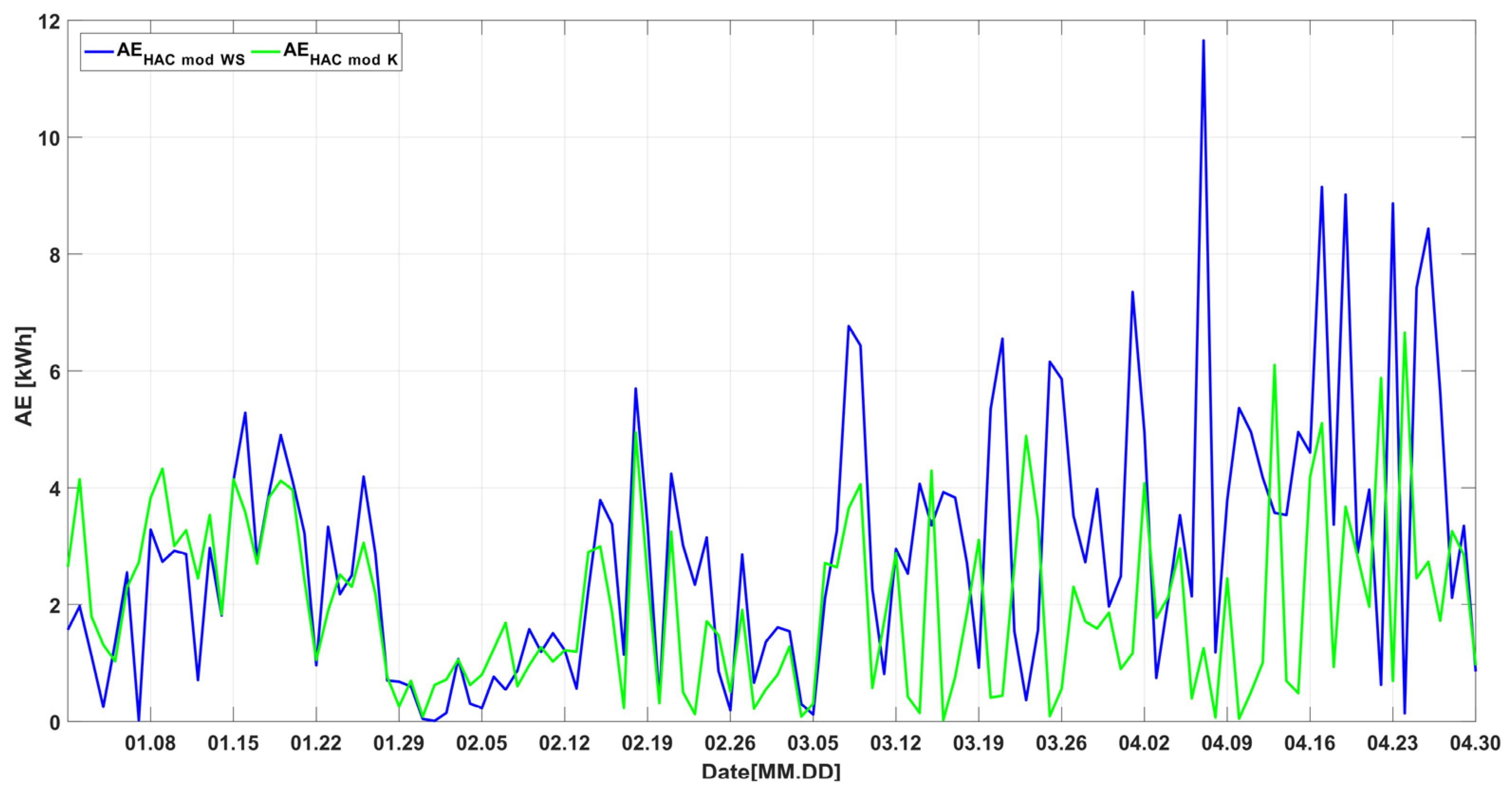
The second stage of the research concerned the tests carried out over the period four months. The carried-out investigation aimed at establishing the influence of the usage of the average daily outdoor temperatures obtained from a meteorological station on the accuracy of the HAC unit model’s calculations. The obtained values of energy consumption (Figure 18) and the calculated absolute error (Figure 19) showed that for the months from January to March, the error deviation values for two considered input datasets were comparable (Table 6 and Table 7). In April, this difference increased significantly. 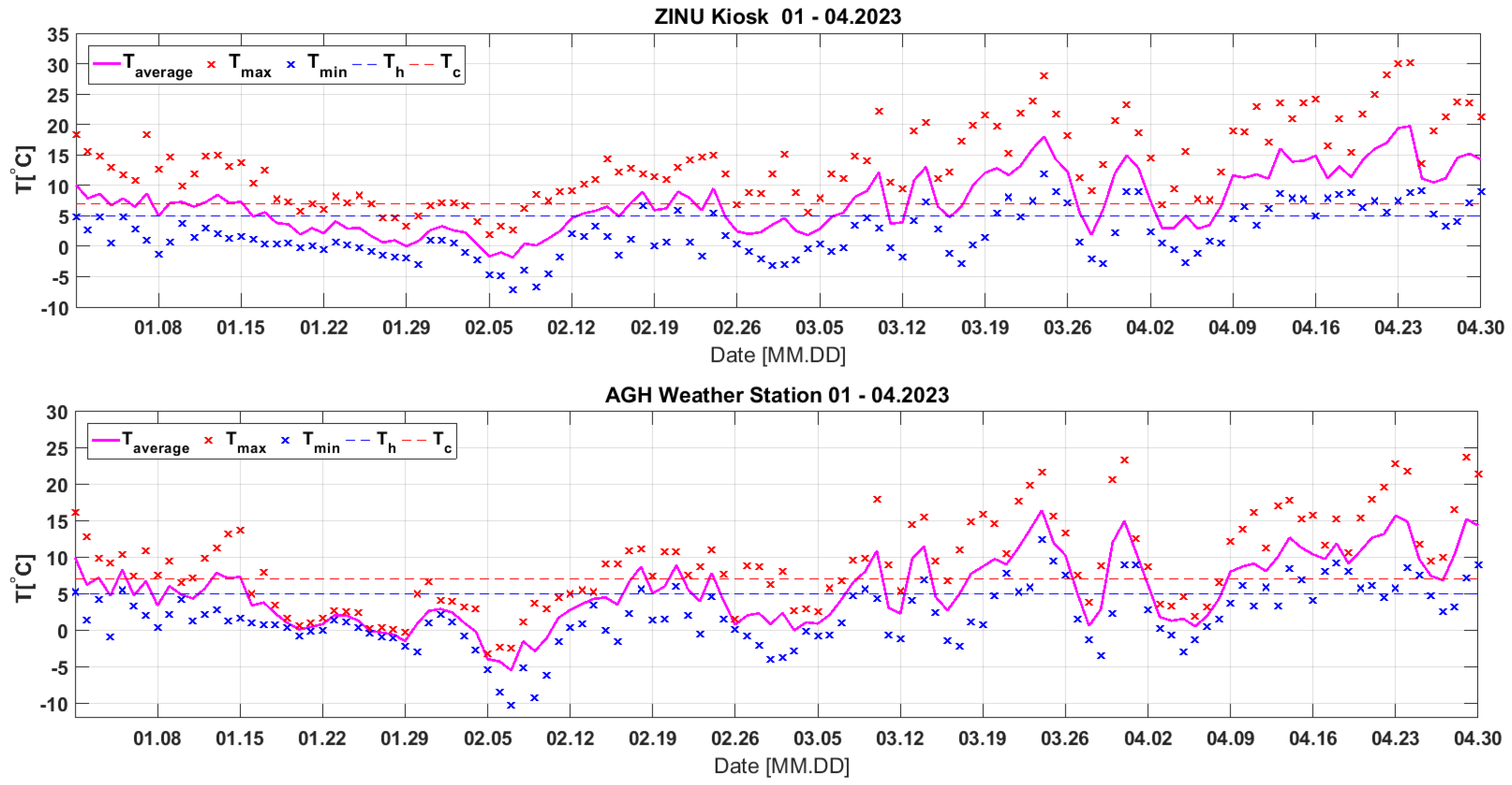The largest spread of the absolute error (Figure 19) occurred for the 97th measurement day (7 April), in which the average temperature measured was 3.4 °C (max.: 7.6 °C; min.: 0.9 °C), and for the meteorological station, it was 1.9 °C (max.: 3.1 °C; min.: 0.5 °C) (Figure 17). The real temperature during the day remained within the temperature range set by the HAC unit thermostat: 4–7 °C (Figure 17, T_h, T_c parameters). This resulted in a relatively low value for the real energy consumption per day of 7.67 kWh (Figure 18). Therefore, the temperature absolute error for that day for the calculations carried out based on the real temperature amounted to 1253 (16.32%), while for the data from the meteorological station, it amounted to 11,655 (151%).

Based on the results of the HAC unit’s total energy consumption (Table 8), the largest error occurred for the month of January for the model based on the measured temperature (77.74 kWh, 15%, Table 9), while for the model based on the temperature from the meteorological station, the error amounted to 68.81 kWh (11.5%, Table 9). The error value in this month was influenced by both the average temperature, which oscillated between 4 and 7 °C (Figure 17), and much greater daily temperature fluctuations, e.g., max. 18.37 °C and min. 1 °C on 1 July. The inaccuracies of the model based on the heat capacity for such a case resulted in a larger error than in case of days with lower dynamics of temperature changes.

The maximum absolute error of the total energy consumption of the automated store feeding system (Table 10) was observed in April (0.34 kWh, 4.7%, Table 11), in which a total of 3146 products were purchased. For the entire measurement period, the absolute error was 0.09 kWh (0.1%), which is fully acceptable.

In the last stage of work on the model, the energy consumption values (Figure 4) of the electrical elements marked as “others” were taken into account. The values of total energy consumption in the individual months and for the entire measurement period (Table 12) were calculated on the basis of the average energy consumption per day, which was equal to 13.5 kWh.

Table 13 shows the total energy consumption of the automated store over a period of 4 months. The maximum error for the model was equal to 59.15 kWh (5.38%)—based on the outdoor temperature measured in April (Table 14)—and 65.78 kWh (5.69%)—based on the temperature from the meteorological station in March (Table 14). The absolute error for the entire period was equal to 68.01 kWh (1.62%) and 90.71 kWh (2.15%), respectively.

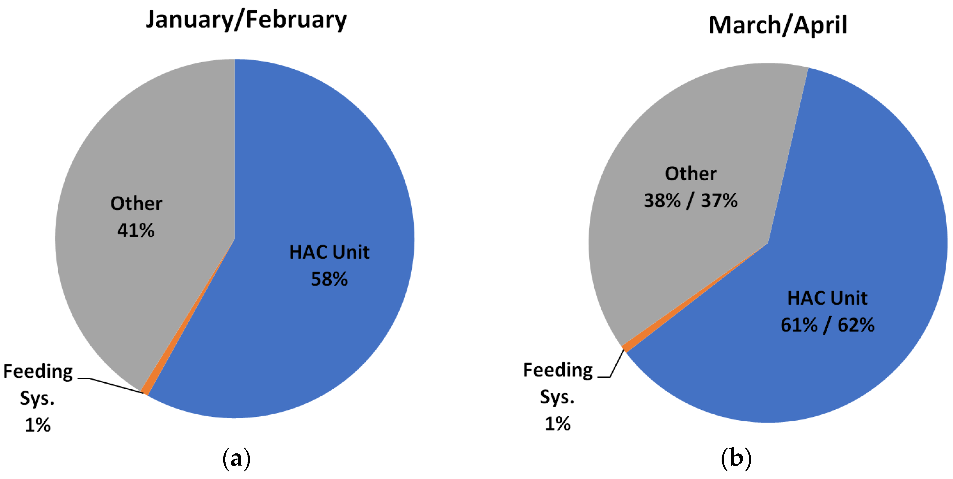
The obtained results of the electrical energy consumption evaluated for the HAC unit (Table 8), the store feeding system (Table 10) and other elements (Table 12) allowed for the analysis of the percentage contribution of the model elements in the overall energy consumption over a period of four months (Figure 20). In January and February, the HAC unit consumed about 58% of the total energy, while in March and April, it was about 62%. The percentage contribution of the feeding system to the energy consumption in the entire period was at the level of approximately 1%.

On the basis of the average CO₂ emission for Poland [37], 742 g/kWh, the values of mass generated for the production of electrical energy were calculated for the individual months of the measurement period (Table 15). The total weight for four months was equal to 3057 kg, while the total cost of generating the energy used by the automated store was EUR 603.

6. Conclusions

The results presented in this paper should be treated as the first to be obtained on the basis of an energy consumption model developed for an automated store with a container structure, taking into account information on the external temperature and the number of products sold, for a single store location. According to the authors’ knowledge, no similar results have been published so far.

The hermetic container structure of the automated store together with the efficient HAC unit with the “defrost” function allowed for the application of the model based on the thermal capacity, on the basis of which electrical energy consumption was calculated.

In case of the considered automated store, contrary to the models of buildings like, e.g., schools, office buildings or houses, it is unnecessary to take into consideration additional factors such as humidity, wind, number of windows, frequency of door opening, etc.

The modelling of the store’s feeding system by means of a simple linear model proved to be sufficient to calculate the value of energy consumption with an accuracy of over 95% (Table 12).

Data from the meteorological station (the store external temperature) allows for the estimation of monthly electrical energy consumption for the HAC unit with an accuracy of 89.5%.The accuracy obtained is sufficient to use the model to forecast energy consumption, CO₂ emission and costs for a potential store locations.

The HAC unit (Figure 20) has the largest contribution to the electrical energy consumption in the analysed time period of four months—approximately 60%. On the other hand, the feeding system, which was switched on when the products are taken, has the smallest contribution of approximately 1%.

To sum up, the main advantages of the proposed solution are a small number of the required model input data, which allows for the quick estimation of energy consumption for any location, easy access to the measurement data, and model implementation that does not require high computational power.

The main disadvantage of the developed solution consists of the fact that the model has currently been verified for one location only for the automated store and, therefore, tests for other locations (latitudes) are planned. Currently, the developed model finds applications in forecasting the costs of energy consumption and gas emissions for a precisely defined type of building structure with an efficient HAC unit.

Future work on the model will concern expanding it to include the application of solar panels as an alternative energy source for the automated store.

References

1. Ekonomou, G.; Menegaki, A.N. The Role of the Energy Use in Buildings in Front of Climate Change: Reviewing a System’s Challenging Future. Energies 2023, 16, 6308. [Google Scholar] [CrossRef]
2. Aguilar, F.J.; Ruiz, R.; Lucasand, M.; Vicente, P.G. Performance Analysis and Optimisation of a Solar On-Grid Air Conditione Energies. Energies 2021, 14, 8054. [Google Scholar] [CrossRef]
3. The Organisation for Economic Co-operation and Development. Future of Cooling: Opportunities for Energy-Efficient Air Conditioning; Annual Report; The Organisation for Economic Co-operation and Development: Paris, France, 2018. [Google Scholar]
4. Liu, H.; Liang, J.; Liu, Y.; Wu, H. Review of Data-Driven Building Energy Prediction. Buildings 2023, 13, 532. [Google Scholar] [CrossRef]
5. Yang, H.; Ran, M.; Zhuang, C. Prediction of Building Electricity Consumption Based on Joinpoint–Multiple Linear Regression. Energies 2022, 15, 8543. [Google Scholar] [CrossRef]
6. Cholewa, T.; Siuta-Olcha, A.; Smolarz, A.; Muryjas, P.; Wolszczak, P.; Guz, U.; Bocian, M.; Balaras, C.A. An easy and widely applicable forecast control for heating systems in existing and new buildings: First field experiences. J. Clean. Prod. 2022, 352, 131605. [Google Scholar] [CrossRef]
7. Haq, I.; Ullah, A.; Khan, S.U.; Khan, N.; Baik, S.W. Sequential learning-based energy consumption prediction model for residential and commercial sectors. Mathematics 2021, 9, 605. [Google Scholar] [CrossRef]
8. Mendoza-Pittí, L.; Calderón-Gómez, H.; Gómez-Pulido, J.M.; Vargas-Lombardo, M.; Castillo-Sequera, J.L.; Blas, C.S. Developing a Long Short-Term Memory-Based Model for Forecasting the Daily Energy Consumption of Heating, Ventilation, and Air Conditioning Systems in Buildings. Appl. Sci. 2021, 11, 6722. [Google Scholar] [CrossRef]
9. Chalapathy, R.; Khoa, N.L.D.; Sethuvenkatraman, S. Comparing multi-step ahead building cooling load prediction using shallow machine learning and deep learning models. Energy Grids Netw. 2021, 28, 100543. [Google Scholar] [CrossRef]
10. Sendra-Arranz, R.; Gutiérrez, A. A long short-term memory artificial neural network to predict daily HVAC consumption in buildings. Energy Build. 2020, 216, 109952. [Google Scholar] [CrossRef]
11. Kusiak, A.; Xu, G.; Zhang, Z. Minimization of energy consumption in HVAC systems with data-driven models and an interior-point method. Energy Convers. 2014, 85, 146–153. [Google Scholar] [CrossRef]
12. Zhang, Q.; Tian, Z.; Ding, Y.; Lu, Y.; Niu, J. Development and evaluation of cooling load prediction models for a factory workshop. Energies 2019, 230, 622–633. [Google Scholar] [CrossRef]
13. Fumo, N.; Rafe Biswas, M.A. Regression analysis for prediction of residential energy consumption. Renew. Sustain. Energy Rev. 2015, 47, 332–343. [Google Scholar] [CrossRef]
14. Qiang, G.; Zhe, T.; Yan, D.; Neng, Z. An improved office building cooling load prediction model based on multivariable linear regression. Energy Build. 2015, 107, 445–455. [Google Scholar] [CrossRef]
15. Alamin, Y.I.; Lvarez, J.D.; Castilla, M.D.M.; Ruano, A. An Artificial Neural Network (ANN) model to predict the electric load profile for an HVAC system. IFAC-PapersOnLine 2018, 51, 26–31. [Google Scholar] [CrossRef]
16. Bünning, F.; Heer, P.; Smith, R.S.; Lygeros, J. Improved day ahead heating demand forecasting by online correction methods. Energy Build. 2020, 211, 109821. [Google Scholar] [CrossRef]
17. Zhu, Q.; Liu, M.; Liu, H.; Zhu, Y. Application of machine learning and its improvement technology in modeling of total energy consumption of air conditioning water system. Math. Biosci. Eng. 2022, 19, 4841–4855. [Google Scholar] [CrossRef]
18. Vo, N.D.; Oh, D.H.; Hong, S.K. Combined approach using mathematical modelling and artificial neural network for chemical industries: Steam methane reformer. Appl. Energy 2019, 255, 113809. [Google Scholar] [CrossRef]
19. Olanrewaju, O.A.; Jimoh, A.A.; Kholopane, P.A. Assessing the energy potential in the South African industry: A combined IDA-ANN-DEA (Index Decomposition Analysis-Artificial Neural Network-Data Envelopment Analysis) model. Energy 2013, 63, 225–232. [Google Scholar] [CrossRef]
20. Paudel, S.; Elmitri, M.; Couturier, S.; Nguyen, P.N.; Kamphuis, R.; Lacarrière, B.; Corre, O.L. A relevant data selection method for energy consumption prediction of low energy building based on support vector machine. Energy Build. 2017, 138, 240–256. [Google Scholar] [CrossRef]
21. Zhong, H.; Wang, J.; Jia, H.; Mu, Y.; Lv, S. Vector field-based support vector regression for building energy consumption prediction. Appl. Energy 2019, 242, 403–414. [Google Scholar] [CrossRef]
22. Ray, M.; Samal, P.; Panigrahi, C.K. Implementation of a Hybrid Technique for the Predictive Control of the Residential Heating Ventilation and Air Conditioning Systems. Eng. Technol. Appl. Sci. Res. 2022, 12, 8772–8776. [Google Scholar] [CrossRef]
23. Li, Q.; Meng, Q.; Cai, J.; Yoshino, H.; Mochida, A. Applying support vector machine to predict hourly cooling load in the building. Appl. Energy 2009, 86, 2249–2256. [Google Scholar] [CrossRef]
24. Sauer, J.; Mariani, V.C.; Coelho, L.S. Extreme gradient boosting model based on improved Jaya optimizer applied to forecasting energy consumption in residential buildings. Evol. Syst. 2022, 13, 577–588. [Google Scholar] [CrossRef]
25. Kamel, E.; Sheikh, S.; Huang, X. Data-driven predictive models for residential building energy use based on the segregation of heating and cooling days. Energy 2020, 206, 118045. [Google Scholar] [CrossRef]
26. Seyedzadeh, S.; Rahimian, F.P.; Oliver, S.; Glesk, I.; Kumar, B. Data driven model improved by multi-objective optimisation for prediction of building energy loads. Autom. Constr. 2020, 116, 103188. [Google Scholar] [CrossRef]
27. Seyedzadeh, S.; Rahimian, F.P.; Rastogi, P.; Glesk, I. Tuning machine learning models for prediction of building energy loads. Sustain. Cities Soc. 2019, 47, 101484. [Google Scholar] [CrossRef]
28. Długosz, M.; Mitkowski, W.; Baranowski, J.; Piątek, P.; Skruch, P. Circuit Systems in Modelling of Thermal Processes in Buildings; Centrum Edukacji w Mechatronice Associated with Unesco International Centre for Engineering Education; Monash University: Clayton, VIC, Austrilia, 2011; pp. 149–152. Available online: https://www.researchgate.net/profile/Marek-Dlugosz/publication/267022663_Uklady_obwodowe_w_modelowaniu_procesow_cieplnych_budynkow/links/5a9c646aa6fdcc3cbacd538f/Uklady-obwodowe-w-modelowaniu-procesow-cieplnych-budynkow.pdf (accessed on 1 July 2023).
29. Deng, K.; Barooah, P.; Mehta, P.G.; Meyn, S.P. Building thermal model reduction via aggregation of states. In Proceedings of the 2010 American Control Conference. ACC 2010, Baltimore, MD, USA, 30 June–2 July 2010; pp. 5118–5123. [Google Scholar]
30. Mitalas, G.P.; Stephenson, D.G. Room thermal response factors. ASHRAE Trans. 1967, 73. Available online: http://web.mit.edu/parmstr/Public/NRCan/rp342.pdf (accessed on 1 July 2023).
31. Clarke, J. Energy Simulation in Building Design; Routledge: London, UK, 2001. [Google Scholar]
32. Crabb, J.A.; Murdoch, N.; Penman, J.M. A simplified thermal response model. Build. Serv. Eng. Res. Technol. 1987, 8, 13–19. [Google Scholar] [CrossRef]
33. Gouda, M.M.; Danaher, S.; Underwood, C.P. Building thermal model reduction using nonlinear constrained optimization. Build. Environ. 2002, 37, 1255–1265. [Google Scholar] [CrossRef]
34. EL3208-0010, EtherCAT Terminal, 8-Channel Analog Input, Temperature, RTD (Pt1000, NTC), 16 bit. Available online: https://www.beckhoff.com/pl-pl/products/i-o/ethercat-terminals/el3xxx-analog-input/el3208.html (accessed on 1 July 2023).
35. EL3403-0010, EtherCAT Terminal, 3-Channel Analog Input, Power Measurement, 500 V AC, 5 A, 16 bit. Available online: https://www.beckhoff.com/en-en/products/i-o/ethercat-terminals/el3xxx-analog-input/el3403-0010.html (accessed on 1 July 2023).
36. Weather Station AGH. Available online: http://meteo.ftj.agh.edu.pl/ (accessed on 1 July 2023).
37. Elektricity Maps, Emission CO2. Available online: https://app.electricitymaps.com/zone/PL (accessed on 1 July 2023).
38. Eurostat—Electricity Prices. Available online: https://ec.europa.eu/eurostat/databrowser/view/nrg_pc_204/default/table?lang=en (accessed on 1 July 2023).
Figure 1. Automated store: (a) illustrative photo from the outside; (b) photo taken inside the store with the components of the feeding system highlighted.
Energies 16 07969 g001
Figure 2. Data visualization in remote monitoring system for an automated store (illustrative representation—screenshot of the operator panel).
Energies 16 07969 g002
Figure 3. Schematic view of the automated retail kiosk’s inner mechanisms: mobile cart and conveyor belts. The gears (14 and 24) were mounted on a mobile cart (3), establishing the link between the shaft of the AC servomotor (23) on one side and a conveyor belt’s passive shaft (12) on the other.
Energies 16 07969 g003
Figure 4. Diagram of model describing energy consumption, energy costs and CO2 mass necessary to generate energy for an automated store.
Energies 16 07969 g004
Figure 5. Electrical energy consumption model of the air conditioning system in the considered automated store implemented in the MATLAB/Simulink environment: thermal model of the store container (1), thermal model of the cooling and heating (HAC) unit (2), and thermostat model (3).
Energies 16 07969 g005
Figure 6. Temperature patterns per day: TOUT Real—measured external temperature, TINT Real—measured temperature inside the store, TINT Mod—internal temperature of the store calculated by the model.
Energies 16 07969 g006
Figure 7. Time histories for 72 h: TOUT_WS—measured external temperature, TOUT_WS—external temperature registered by the meteorological station, TINT_Real—temperature measured inside the store, TINT_Mod WS—temperature inside the store estimated from the assumed model on the basis of the data from the meteorological station.
Energies 16 07969 g007
Figure 8. Power consumed by the HAC unit.
Energies 16 07969 g008
Figure 9. The number of products collected from the store in a 24 h period.
Energies 16 07969 g009
Figure 10. Measurement of power consumed by the feeding system over a 24 h period.
Energies 16 07969 g010
Figure 11. Energy consumption per product.
Energies 16 07969 g011
Figure 12. Power calculated by the model for the feeding system PF MOD 0 and the relative error based on the difference between the measured power and power calculated by Mod 0 for a 24 h period.
Energies 16 07969 g012
Figure 13. Scheme of the feeding system model implemented in the MATLAB/Simulink environment.
Energies 16 07969 g013
Figure 14. The power PF Mod 1 calculated from the model for the store’s feeding system and the relative error commutated on the basis of the difference between the measured power and power value calculated from the model Mod 1 for the period of 24 h.
Energies 16 07969 g014
Figure 15. The number of products downloaded from the store in a time period of 72 h, power PF Real measured on the real object, power PF Mod 0 calculated by the model Mod 0 (the first version), and power PF Mod 1 calculated by the model Mod 1 (the second version).
Energies 16 07969 g015
Figure 16. Relative error calculated on the basis of the difference between the measured power value and the power calculated by the model Mod 1 for a time period of 72 h.
Energies 16 07969 g016
Figure 17. Daily changes in the external temperature, based on the data recorded by the measurement system of the automated ZINU store and the AGH Weather Station. Tavarage—average temperature; Tmax—maximum temperature; Tmin—minimum temperature; Tc, Th—parameters of the HAC unit thermostat.
Energies 16 07969 g017
Figure 18. Daily energy consumption by the HAC unit, where: EHAC Real—measured daily energy consumption, EHAC Mod K—daily energy consumption calculated by the model for the temperature measured by the store measurement system, EHAC Mod WS—daily energy consumption calculated by the model for data from the meteorological station.
Energies 16 07969 g018
Figure 19. Absolute error of daily energy consumption for the model, where: AEHAC Mod WS—error of daily energy consumption for temperature from the meteorological station, AEHAC Mod K—error of daily energy consumption for temperature registered by the store measurement system.
Energies 16 07969 g019
Figure 20. Percentage of electrical energy consumption for individual elements of the model over the four measurement months: (a) for January and February, (b) for March and April.
Energies 16 07969 g020