

Sliding Mode Predictive Current Control for Single-Phase H-Bridge Converter with Parameter Robustness

Abstract
:1. Introduction
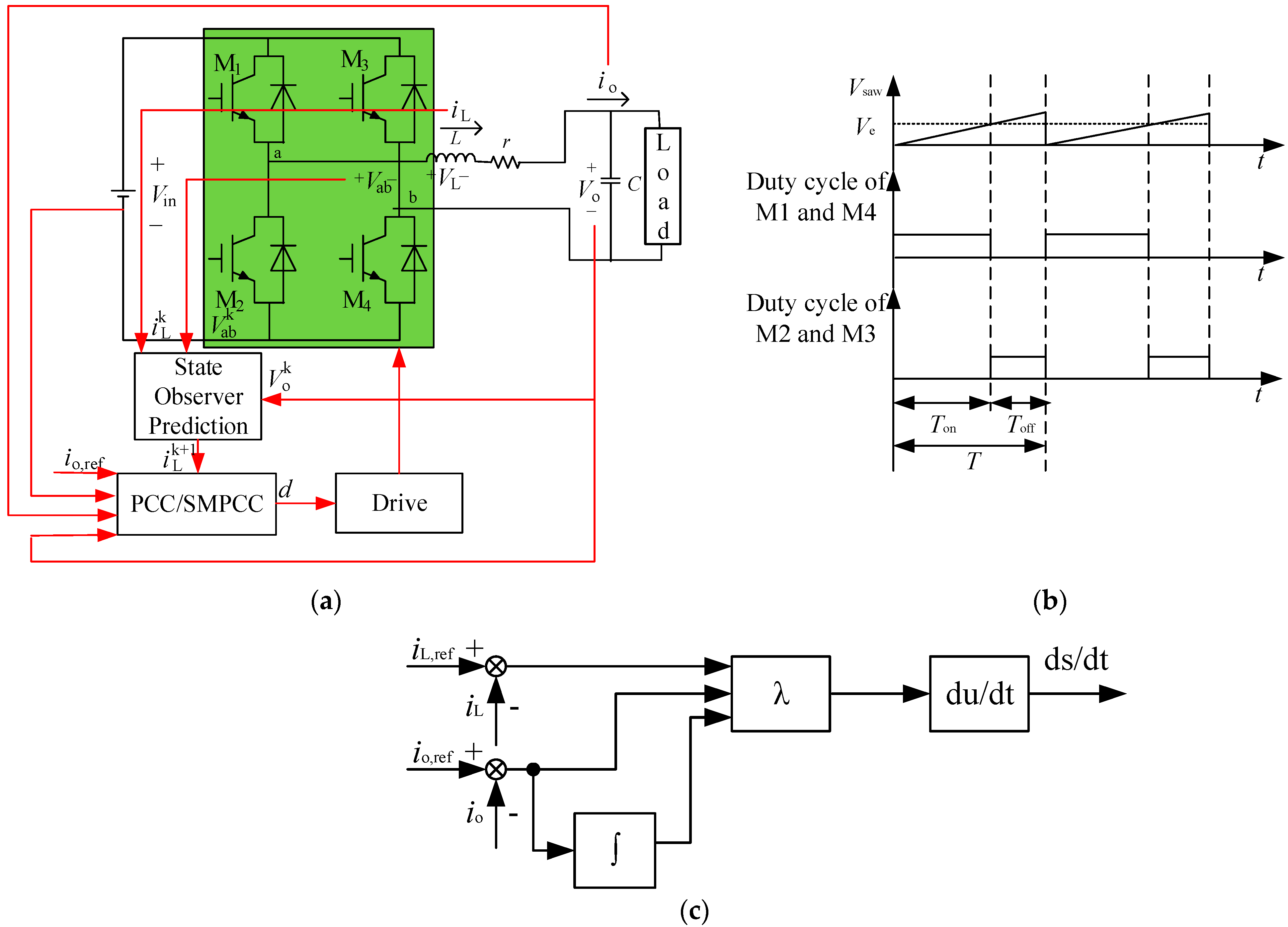
2. Sliding Mode Predictive Current Control
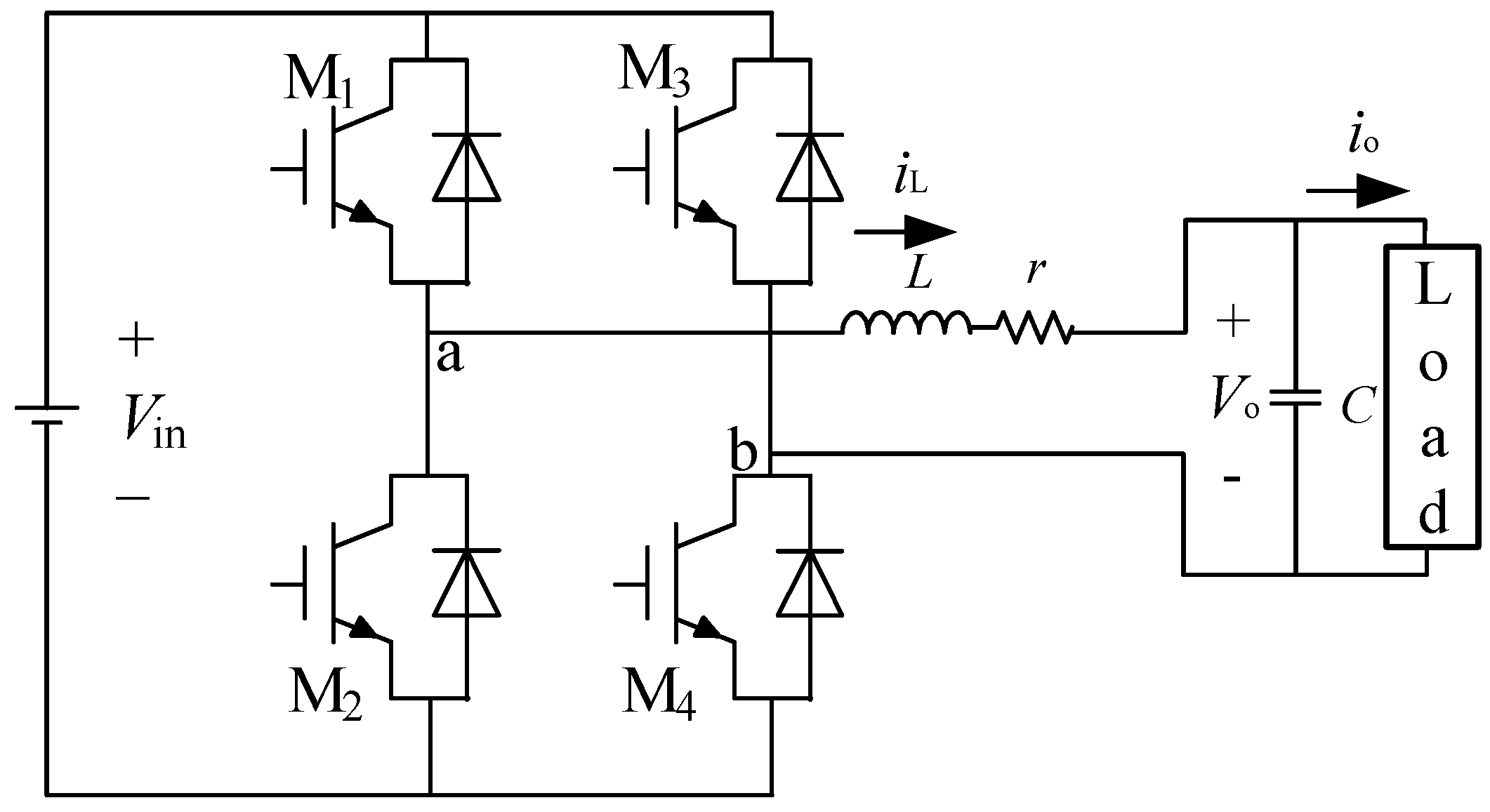
2.1. Establishment of System Model
2.2. Design of Sliding Mode Controller
2.3. System Stability Analysis
2.4. Traditional PCC and Control Delay Compensation
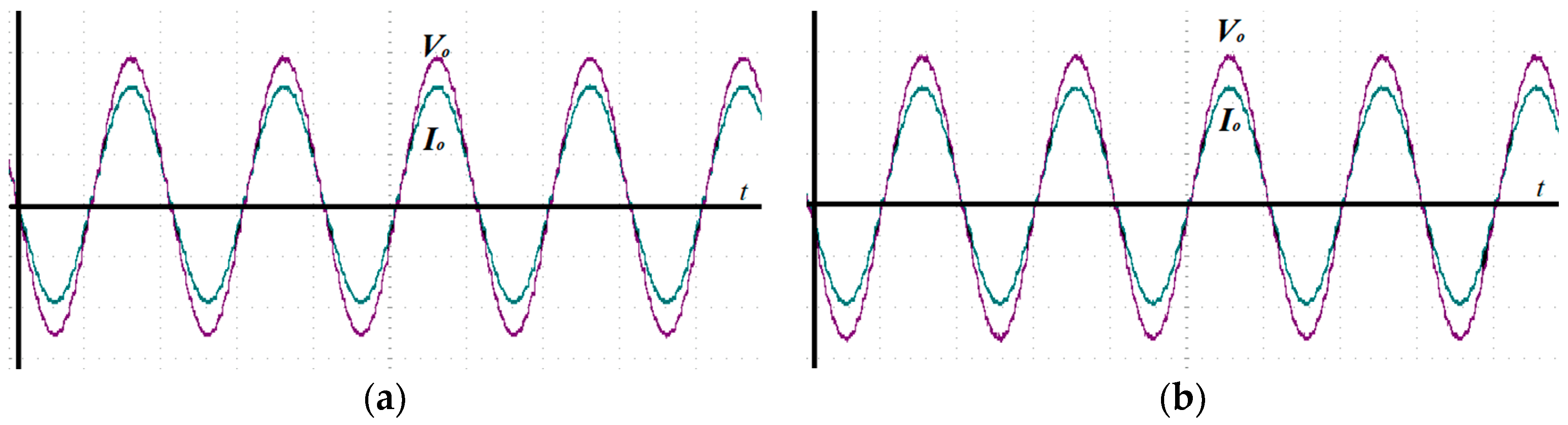
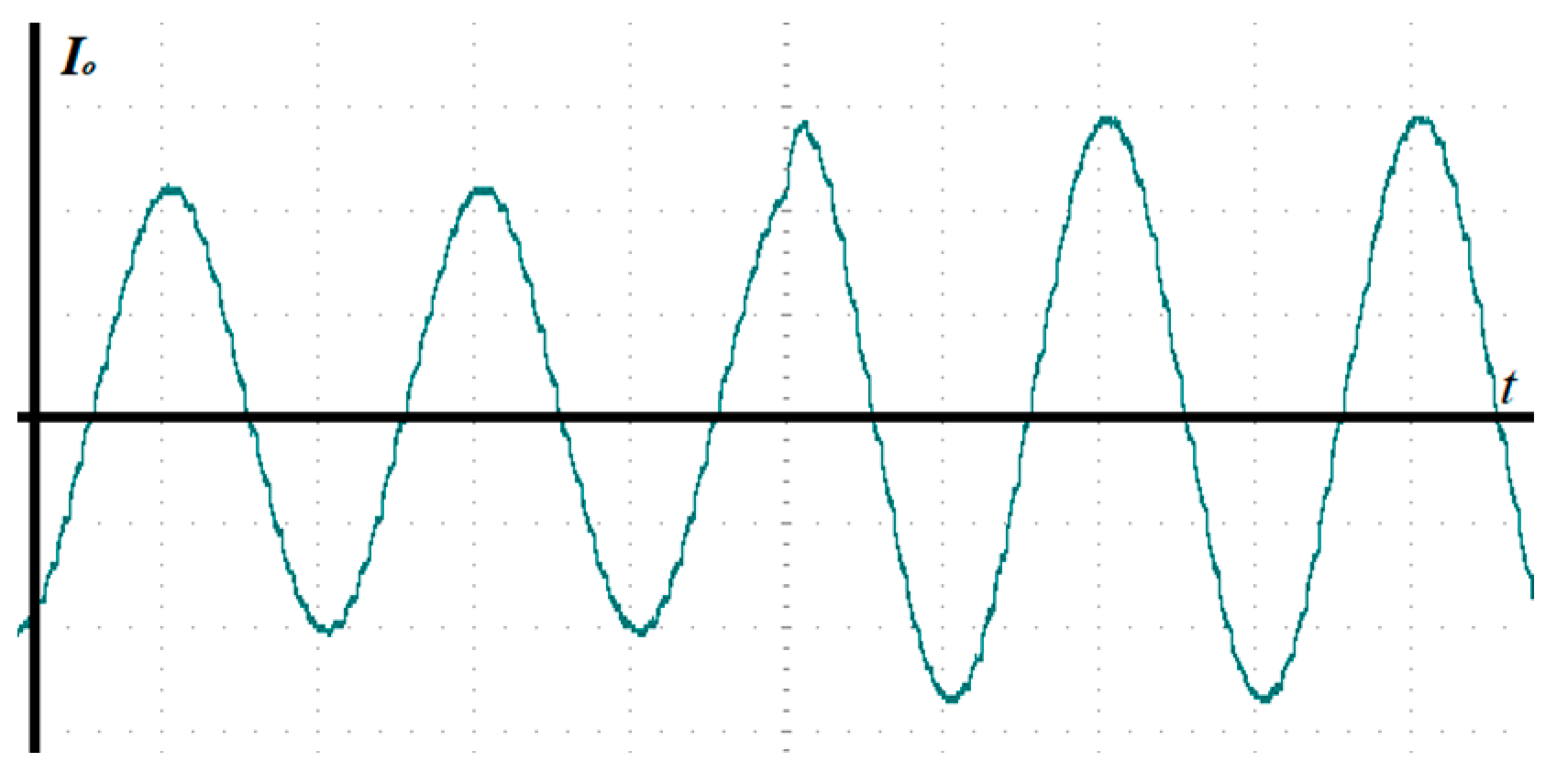
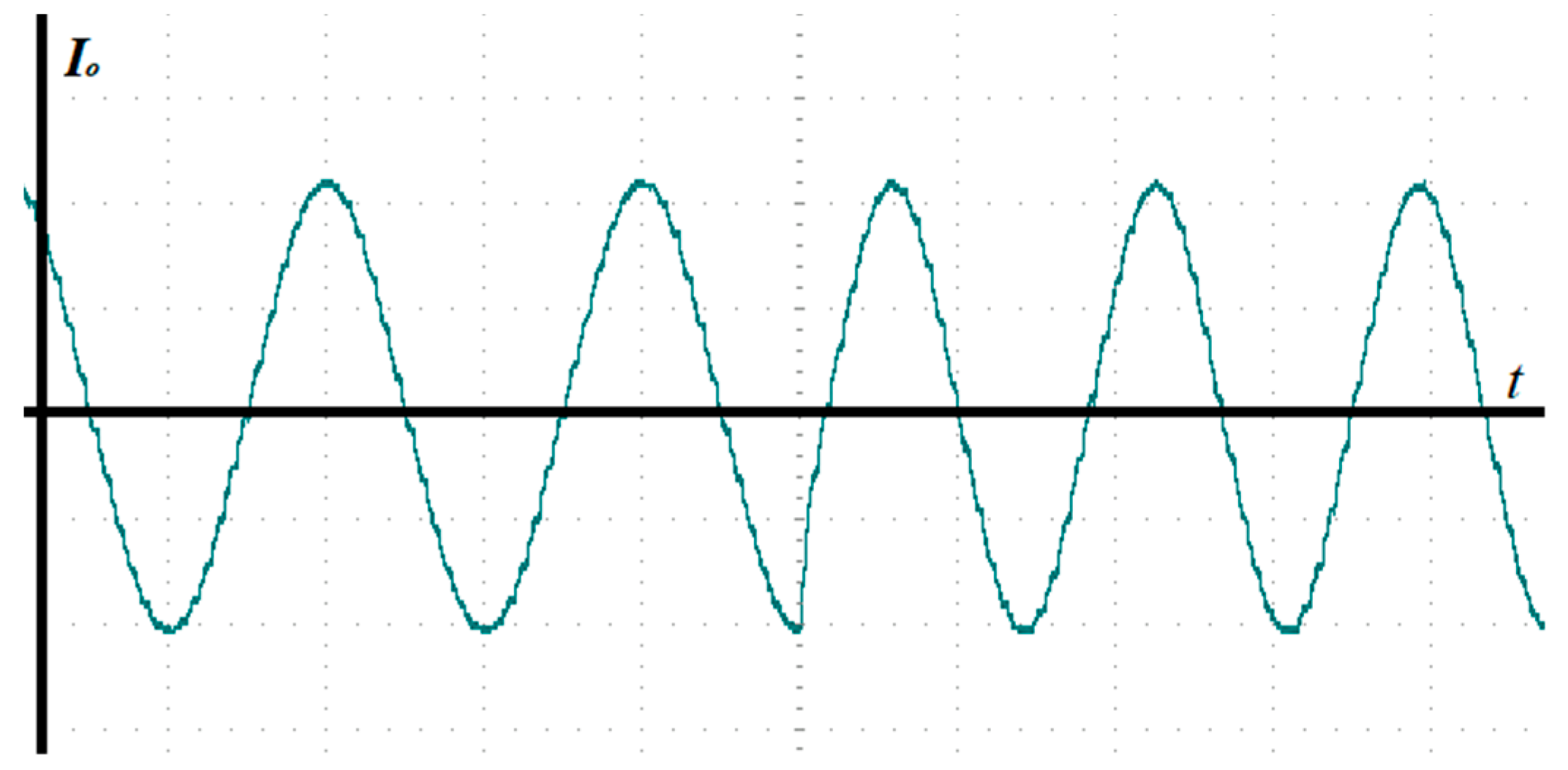
3. Results
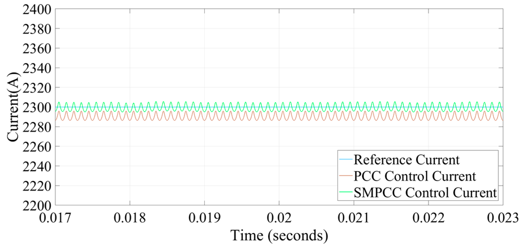
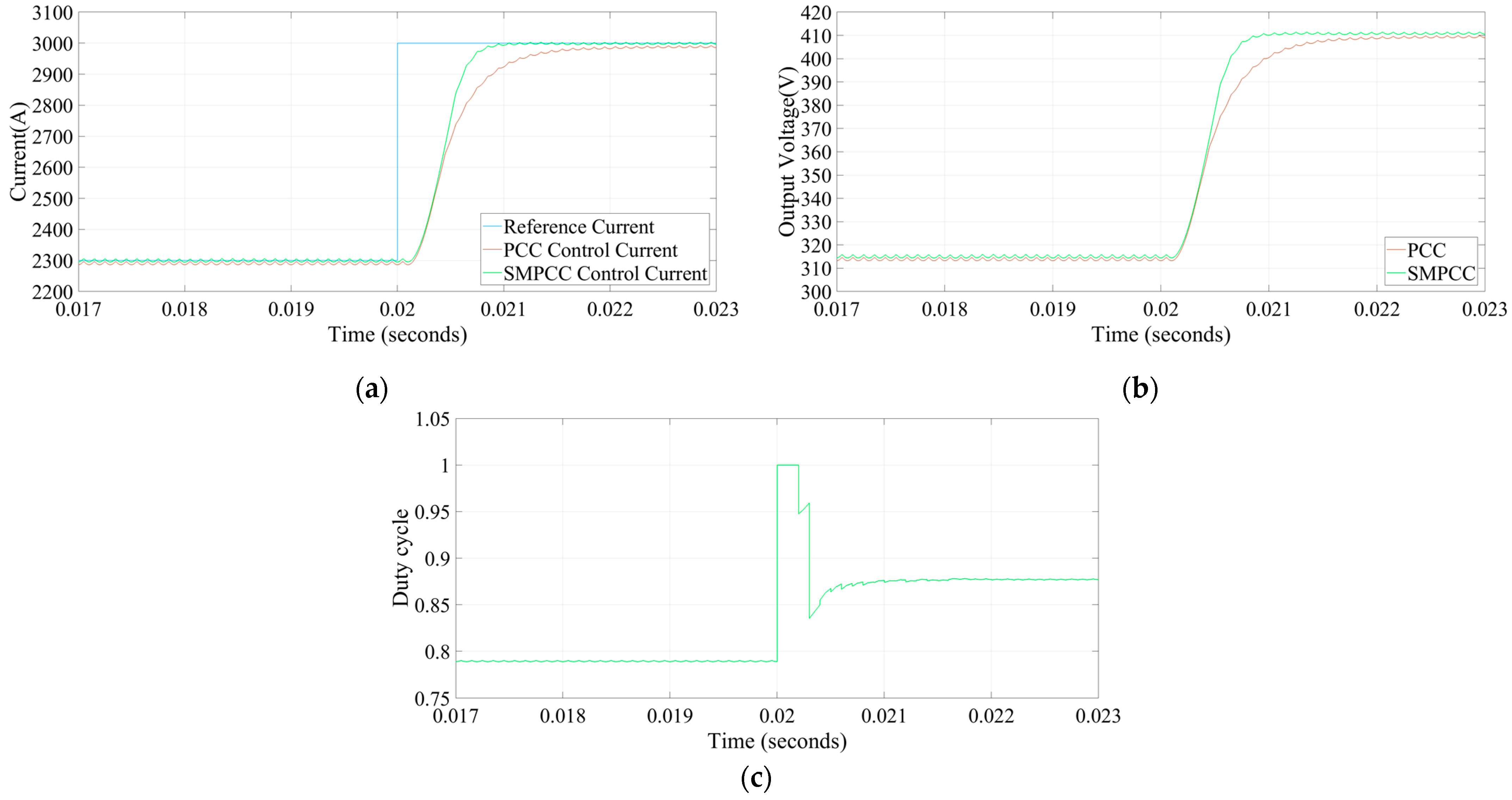
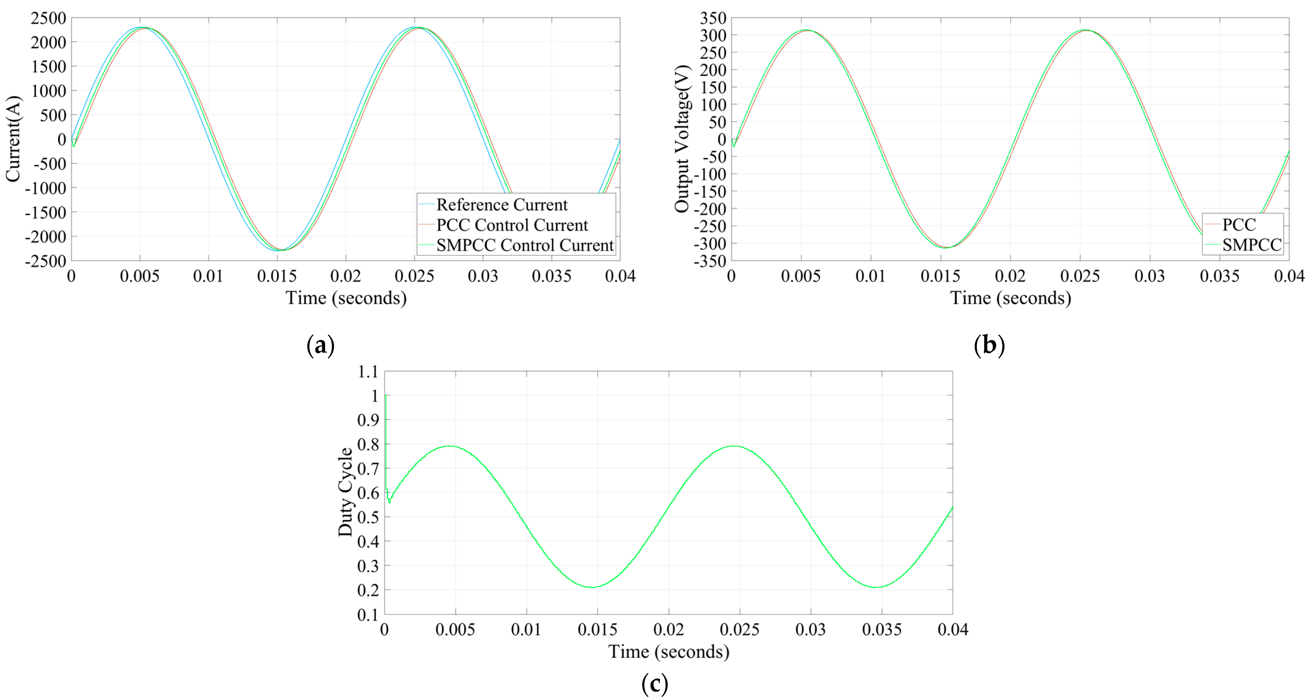
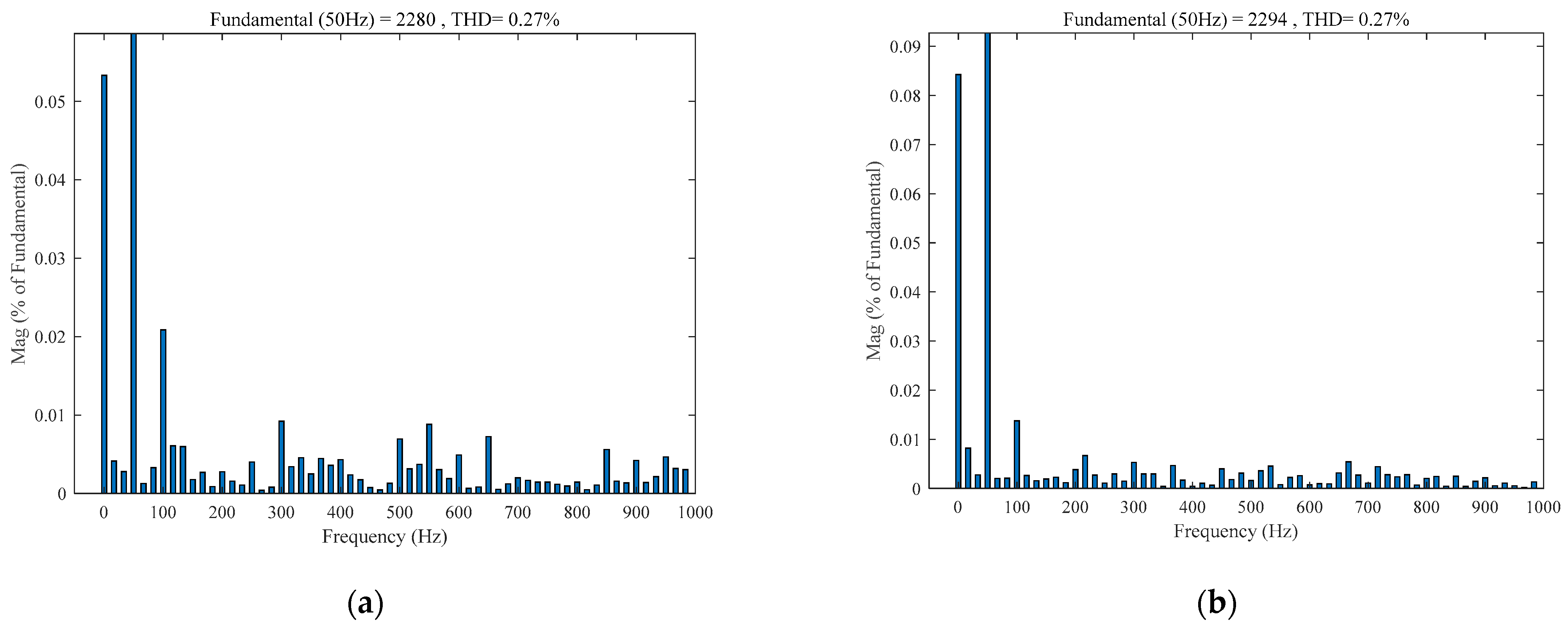
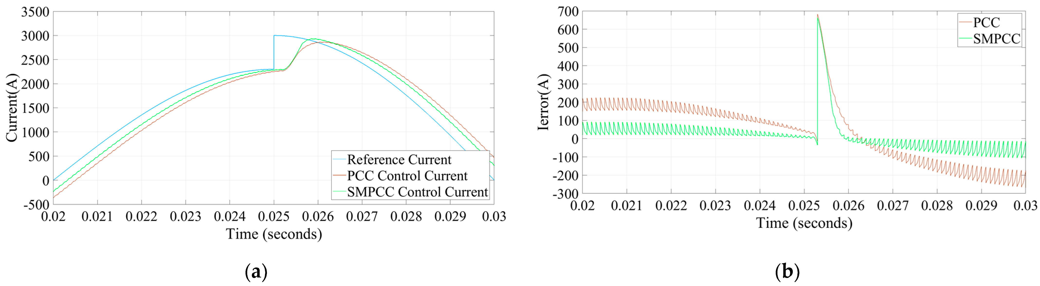
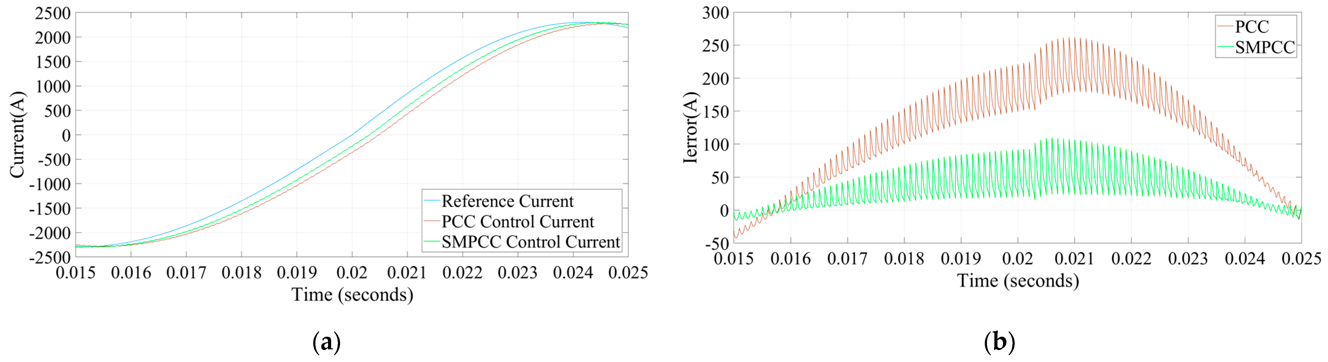
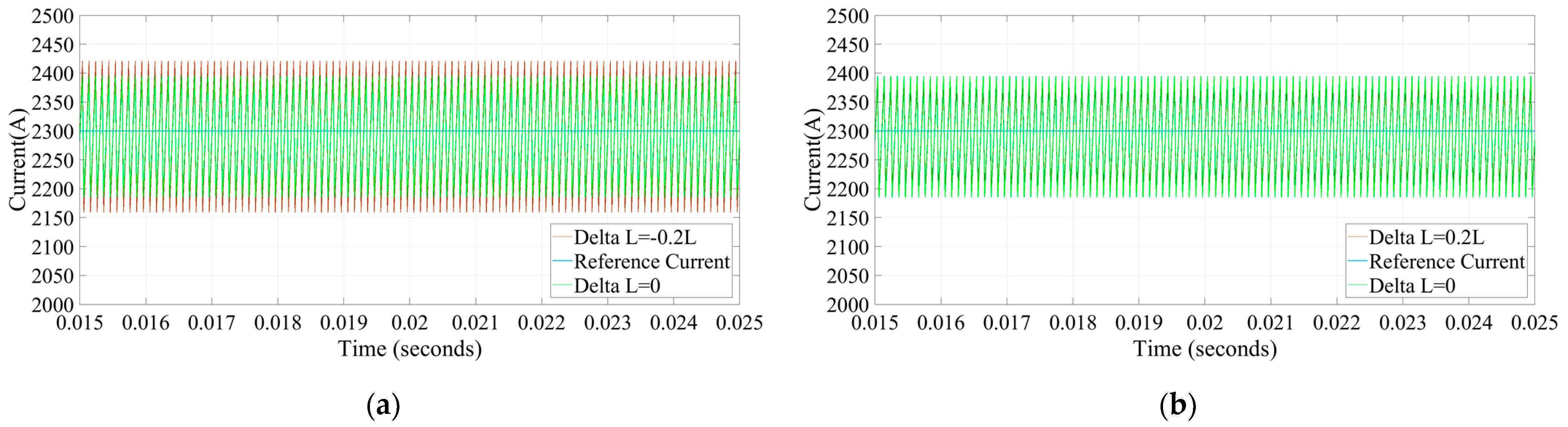
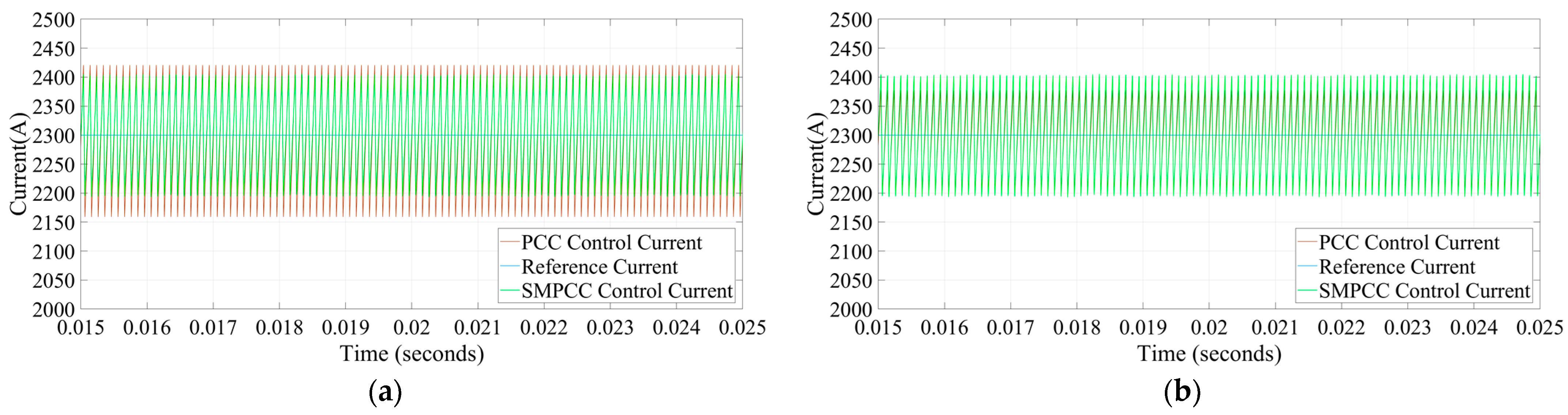
3.1. Simulation
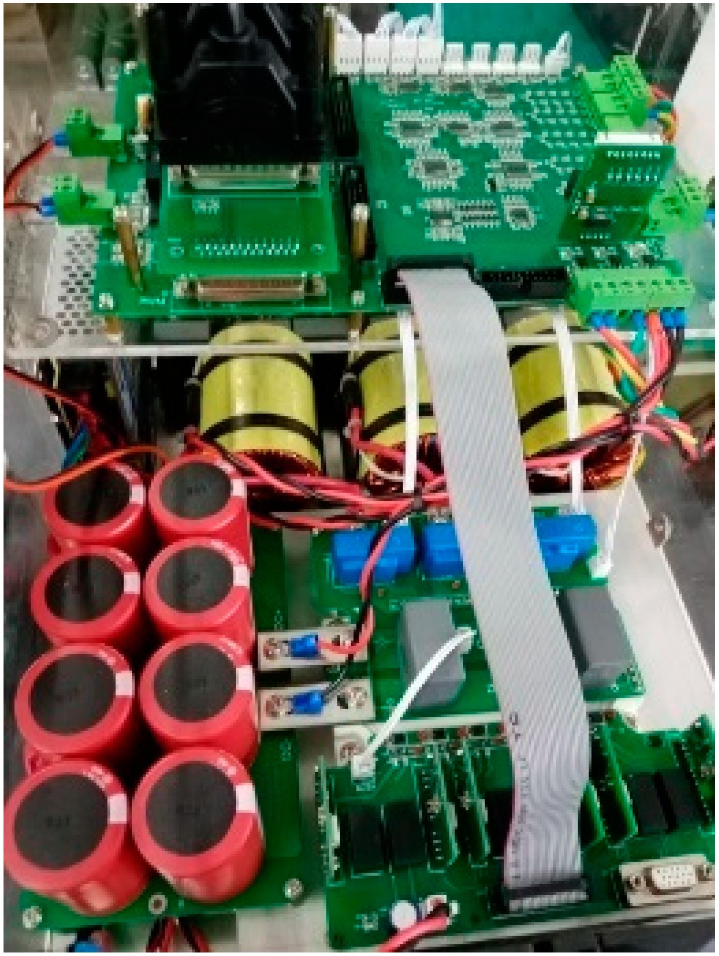
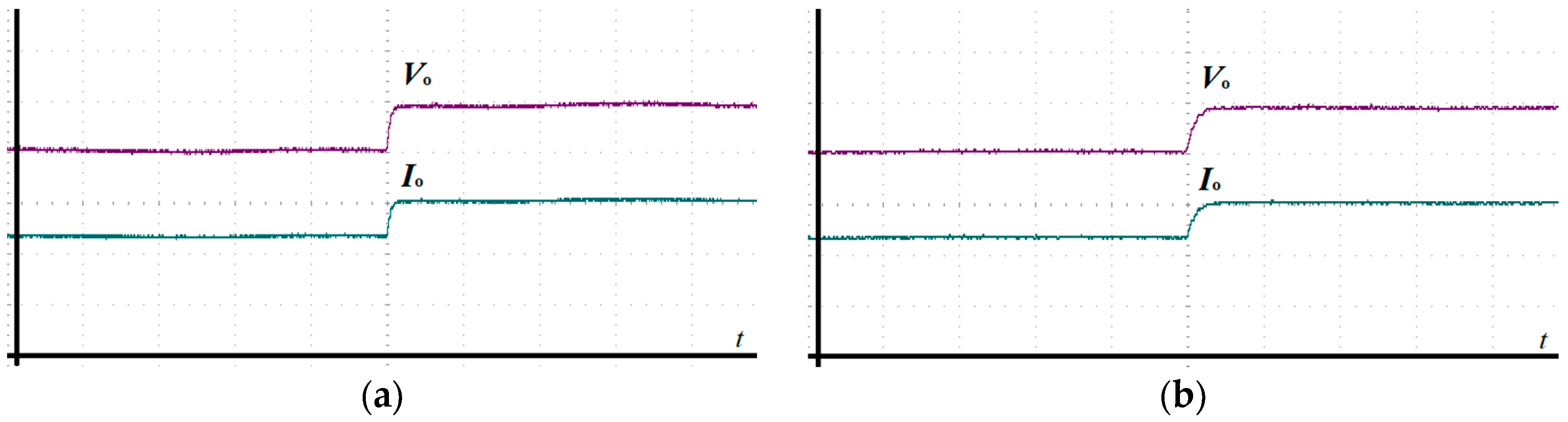
3.2. Experimental
4. Conclusions
Author Contributions
Funding
Data Availability Statement
Conflicts of Interest
References
- Pandit, D.; Nguyen, N.; Elsaiah, S.; Mitra, J. Reliability evaluation of solar PV system incorporating insolation-dependent failure rates. In Proceedings of the International Conference on Smart Energy Systems and Technologies (SEST), Vaasa, Finland, 6–8 September 2021. [Google Scholar]
- Zhao, Y.; Gong, S.; Zhang, C.; Ge, M.; Xie, L. Performance analysis of a solar photovoltaic power generation system with spray cooling. Case Stud. Therm. Eng. 2022, 29, 1–12. [Google Scholar] [CrossRef]
- Vo, T.T.E.; Ko, H.; Huh, J.; Park, N. Overview of possibilities of solar floating photovoltaic systems in the offshore industry. Energies 2021, 14, 6988. [Google Scholar] [CrossRef]
- Jassim, A.K.; Ateeq, A.A. Wind energy applied as a sustainable technology to produce electrical energy in Basra. In Proceedings of the 5th International Scientific Conference on Advanced Engineering Technologies (ISC-AET) 2020 (Virtual Conference), Basra, Iraq, 18–19 August 2020. [Google Scholar]
- Tong, Y.; Fan, W.; Liu, Z. Influence of wind power generation system accessing to traction power supply system on power quality. In Proceedings of the 5th International Conference on Electrical Engineering and Information Technologies for Rail Transportation (EITRT) 2021, Qingdao, China, 21–23 October 2021. [Google Scholar]
- Saadaoui, F.; Youcef, M.; Mammar, K. Energy management of a hybrid energy system (PV/PEMFC and lithium battery) using macroscopic energy representation. In Proceedings of the Artificial Intelligence and Heuristics for Smart Energy Efficiency in Smart Cities, Tipasa, Algeria, 24–26 November 2021. [Google Scholar]
- Kumar, A.; Mishra, V.M.; Ranjan, R. A survey on hybrid renewable energy system for standalone and grid connected applications: Types, storage options, trends for research and control strategies. WSEAS Trans. Electron. 2020, 11, 80–85. [Google Scholar] [CrossRef]
- Chen, F.; Cai, X.S. Design of feedback control laws for switching regulators based on the bilinear large signal model. IEEE Trans. Power Electron. 1990, 5, 236–240. [Google Scholar] [CrossRef]
- Malesani, L.; Spiazzi, R.G.; Tenti, P. Performance optimization of Cuk converters by sliding-mode control. IEEE Trans. Power Electron. 1995, 10, 302–309. [Google Scholar] [CrossRef]
- Ramirez, H.S.; Esteban, M.G.; Zinober, A.S.I. Dynamical adaptive pulse-width-modulation control of DC-to-DC power converters: A backstepping approach. Int. J. Control 1996, 65, 205–222. [Google Scholar] [CrossRef]
- Xi, Y.; Li, D.W.; Lin, S. Model predictive control—Status and challenge. Acta Autom. Sin. 2013, 39, 222–236. [Google Scholar] [CrossRef]
- Ma, J.; Song, W.; Wang, S.; Feng, X. Deadbeat predictive direct power control of single-phase three-level pulse rectifiers. Proc. Chin. Soc. Electr. Eng. 2015, 35, 935–943. [Google Scholar] [CrossRef]
- Yu, B.; Chang, L. Improved predictive current controlled PWM for single-phase grid-connected voltage source inverters. In Proceedings of the 2005 IEEE 36th Power Electronics Specialists Conference, Dresden, Germany, 16 June 2005. [Google Scholar]
- Zhang, X.; Hou, B.; Mei, Y. Deadbeat predictive current control of permanent-magnet synchronous motors with stator current and disturbance observer. IEEE Trans. Power Electron. 2016, 32, 3818–3834. [Google Scholar] [CrossRef]
- Zhang, C.; Wu, G.; Rong, F.; Feng, J.; Jia, L.; He, J.; Huang, S. Robust fault-tolerant predictive current control for permanent magnet synchronous motors considering demagnetization fault. IEEE Trans. Ind. Electron. 2018, 65, 5324–5334. [Google Scholar] [CrossRef]
- Mohamed, Y.A.I.; El-Saadany, E.F. Robust high bandwidth discrete-time predictive current control with predictive internal model—A unified approach for voltage-source PWM converters. IEEE Trans. Power Electron. 2008, 23, 126–136. [Google Scholar] [CrossRef]
- Nishida, Y.; Miyashita, O.; Haneyoshi, T.; Tomita, H.; Maeda, A. A predictive instantaneous-current PWM controlled rectifier with AC-side harmonic current reduction. IEEE Trans. Ind. Electron. 1997, 44, 337–343. [Google Scholar] [CrossRef]
- Wu, T.F.; Sun, K.H.; Kuo, C.L.; Chang, C.H. Predictive current controlled 5-kW single-phase bidirectional inverter with wide inductance variation for DC-microgrid applications. IEEE Trans. Power Electron. 2010, 25, 3076–3084. [Google Scholar] [CrossRef]
- Wu, Z.; Zou, Y.; Zhang, Z.; Zhang, Y. Adaptive predictive controller of supply current applied in single-phase PWM rectifier. Trans. China Electrotech. Soc. 2010, 25, 73–79. [Google Scholar]
- Yang, L.; Yang, S.; Zhang, W.; Chen, Z.; Xu, L. The improved deadbeat predictive current control method for single-phase PWM rectifiers. Proc. Chin. Soc. Electr. Eng. 2015, 35, 5842–5850. [Google Scholar] [CrossRef]
- Cavallo, A.; Canciello, G.; Russo, A. Supervised energy management in advanced aircraft applications. In Proceedings of the 2018 European Control Conference (ECC), Limassol, Cyprus, 12–15 June 2018; pp. 2769–2774. [Google Scholar] [CrossRef]
- Li, H.; Chen, X.; Zhang, H.; Cui, X. High-precision speed control for low-speed gimbal systems using discrete sliding mode observer and controller. IEEE J. Em. Sel. Top. P. 2022, 10, 2871–2880. [Google Scholar] [CrossRef]
- Dehkordi, N.M.; Sadati, N.; Hamzeh, M. A robust backstepping high-order sliding mode control strategy for grid-connected DG units with harmonic/interharmonic current compensation capability. IEEE Trans. Sustain. Energ. 2017, 8, 561–572. [Google Scholar] [CrossRef]
- Le, J.Y.; Xie, Y.X.; Ji, Y.P.; Zhang, Z. Sliding-mode variable-structure control of CCM buck converter based on exact feedback linearization. J. South China Univ. Technol. 2012, 40, 130–135+160. [Google Scholar] [CrossRef]


Disclaimer/Publisher’s Note: The statements, opinions and data contained in all publications are solely those of the individual author(s) and contributor(s) and not of MDPI and/or the editor(s). MDPI and/or the editor(s) disclaim responsibility for any injury to people or property resulting from any ideas, methods, instructions or products referred to in the content. |
© 2023 by the authors. Licensee MDPI, Basel, Switzerland. This article is an open access article distributed under the terms and conditions of the Creative Commons Attribution (CC BY) license (https://creativecommons.org/licenses/by/4.0/).
Share and Cite
Zheng, W.; Sun, Z.; Liu, B. Sliding Mode Predictive Current Control for Single-Phase H-Bridge Converter with Parameter Robustness. Energies 2023, 16, 781. https://doi.org/10.3390/en16020781
Zheng W, Sun Z, Liu B. Sliding Mode Predictive Current Control for Single-Phase H-Bridge Converter with Parameter Robustness. Energies. 2023; 16(2):781. https://doi.org/10.3390/en16020781
Chicago/Turabian StyleZheng, Wei, Zhaolong Sun, and Baolong Liu. 2023. "Sliding Mode Predictive Current Control for Single-Phase H-Bridge Converter with Parameter Robustness" Energies 16, no. 2: 781. https://doi.org/10.3390/en16020781