Digital Twin for Experimental Data Fusion Applied to a Semi-Industrial Furnace Fed with H₂-Rich Fuel Mixtures

Abstract

The objective of this work is to build a Digital Twin of a semi-industrial furnace using Gaussian Process Regression coupled with dimensionality reduction via Proper Orthogonal Decomposition. The Digital Twin is capable of integrating different sources of information, such as temperature, chemiluminescence intensity and species concentration at the outlet. The parameters selected to build the design space are the equivalence ratio and the benzene concentration in the fuel stream. The fuel consists of a ${\mathrm{H}}_2$/${\mathrm{CH}}_4$/$\mathrm{CO}$ blend, doped with a progressive addition of ${\mathrm{C}}_6{\mathrm{H}}_6$. It is an ${\mathrm{H}}_2$-rich fuel mixture, representing a surrogate of a more complex Coke Oven Gas industrial mixture. The experimental measurements include the flame temperature distribution, measured on a $6\times 8$ grid using an air-cooled suction pyrometer, spatially resolved chemiluminescence measurements of ${\mathrm{OH}}^{*}$ and ${\mathrm{CH}}^{*}$, and the species concentration (i.e., $\mathrm{NO}$, ${\mathrm{NO}}_2$, $\mathrm{CO}$, ${\mathrm{H}}_2\mathrm{O}$, ${\mathrm{CO}}_2$, ${\mathrm{O}}_2$) measured in the exhaust gases. The GPR-based Digital Twin approach has already been successfully applied on numerical datasets coming from CFD simulations. In this work, we demonstrate that the same approach can be applied on heterogeneous datasets, obtained from experimental measurements.

1. Introduction

The need for the rapid decarbonization of the global economy requires the development of new combustion systems that are both efficient and flexible, to allow the use of new zero-carbon fuels such as hydrogen and ammonia [1].

These requirements, coupled with the necessity of limiting the production of harmful pollutants, impose strict operating conditions on the combustion systems. This means that the design and control of these systems is crucial, and the margin of error is limited.

For this reason, the model of trial-and-error employed for the design of a traditional combustion system is both too time-consuming and error prone to be applied on the development of new combustion designs.

Luckily, the recent developments in machine-learning techniques and the increasing availability of data offer various tools that can be exploited in the design and operation of combustors.

In particular, the development of Digital Twins (DTs) has been increasingly regarded as a way to substantially improve both the knowledge of industrial systems and their control [2,3,4]. The DT is defined as a digital representation of a physical object that can closely simulate its behavior in the real environment [2,4]. The DT can help in the design, production and service phases of a product. In the design phase, the DT is useful in the iterative optimization and the virtual evaluation, while in the production phase it can be employed for real-time monitoring, control and prediction. Finally, in the service phase, the DT can be used to forecast the product’s maintenance [2,3].

Crucially, the DT has to provide a real-time prediction of the state of its physical counterpart, so that it can supply constant reference values.

This requirement generally excludes Computational Fluid Dynamics (CFD) simulations as techniques to rely on building DTs because the computing time is not negligible, even for relatively simple geometries.

Instead, data-driven regression models, such as linear regression, Gaussian Process Regression (GPR) and Neural Networks (NNs), are particularly suited for this kind of application because the training phase is distinct from the prediction phase. This means that the training phase, however long, can be performed offline while the trained model can predict the system’s state almost instantaneously.

Among these regression methods, the GPR offers a number of advantages with respect to the other regression models. In particular, it is a nonlinear technique based on Bayesian inference with a limited amount of hyperparameters to tune. This probabilistic framework means that the predictions are complemented with the model’s uncertainty [5].

Moreover, the GPR performs well with sparse datasets. The availability of sparse datasets is often the case when dealing with reactive systems because the amount of operating conditions explored is limited by the computational cost (for CFD simulations) or the operating cost (for experimental campaigns).

Other important tools to build DTs are dimensionality reduction techniques, in particular the Proper Orthogonal Decomposition (POD) [6]. The POD is a linear technique capable of finding a low-dimensional representation of the system without losing important information. This allows for greatly reducing the complexity of the model while maintaining high accuracy in the prediction.

Recently, the GPR and POD approach has been employed to develop a numerical DT of a semi-industrial furnace [7], while the POD coupled with sparse sensing was used to develop a hybrid numerical-experimental DT of the same furnace [8].

However, in some situations, it is not possible to rely on the availability of numerical data to build a DT. For example, numerical simulations of highly turbulent reacting flows still do not provide accurate predictions of pollutants and stability limits [9]. Moreover, the use of state-of-the-art Large Eddy Simulation combustion models is often too expensive to be applied to industrial facilities [10].

In these cases, an experimental campaign is often carried out with different measuring instruments to characterize the combustion system. This usually produces various datasets with vastly different spatial scales (the pressure field obtained using pressure probes has a much lower spatial resolution than a velocity field measured using particle image velocimetry, for example).

The objective of this work is to develop a DT of the ULB semi-industrial furnace which relies solely on experimental data. The DT is capable of integrating different data streams and it provides in real time the prediction of temperature, chemiluminescence and species concentration, for different degrees of equivalence ratio and benzene doping in the fuel blend. To achieve this, the experimental data are first projected into the low-dimensional space using POD. Then, the regression is performed using GPR in the low-dimensional manifold. Finally, the prediction can be obtained by projecting the solution found by the GPR model in the original space.

The experimental setup is outlined in Section 2, while the methodology for the development of the DT is explained in more detail in Section 3. The results are shown in Section 4 and discussed in Section 5.

2. Experimental Setup

The experimental data have been collected in a semi-industrial furnace, fed with ${\mathrm{H}}_2$/${\mathrm{CH}}_4$/$\mathrm{CO}$ fuel mixtures doped with ${\mathrm{C}}_6{\mathrm{H}}_6$. Detailed information about the experimental setup and measurement techniques are provided in previous publications [11,12], while the dataset used in this work has been published in [13].

However, some key features of the experimental set-up are also summarized below, along with the specific operating conditions used for this dataset.

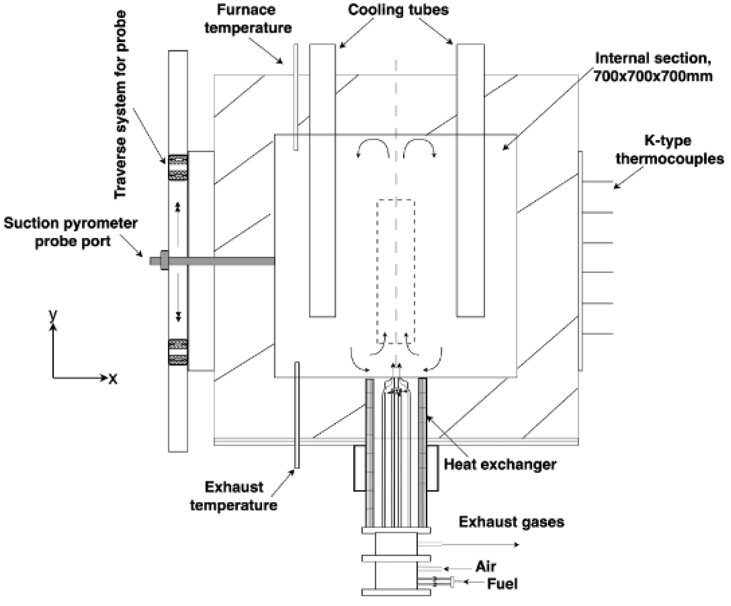
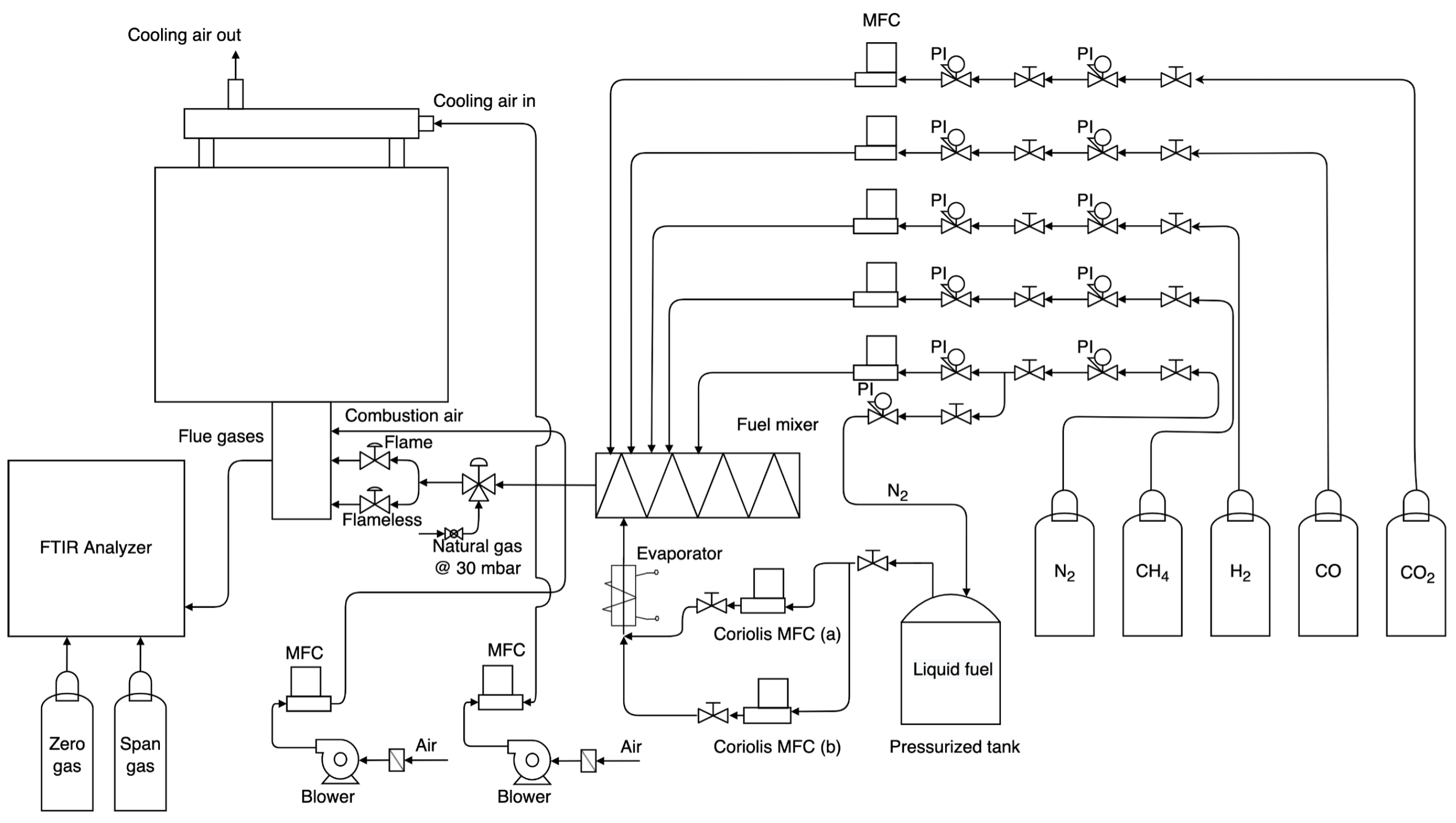
The combustion furnace used in this work consists of an insulated combustion chamber. Figure 1 shows the schematic diagram of the vertical cross-section of the furnace-burner assembly, while Figure 2 shows a schematic representation of the test bench.

The furnace has a cubic shape (1100 × 1100 × 1100 mm), and it is internally insulated with a 200 mm thick high-temperature (1300 °C) ceramic foam layer, which limits the heat lost through the walls. Therefore, the resulting inner dimensions of the combustion chamber are: 700 × 700 × 700 mm.

The furnace is equipped with an air cooling system, which consists of four cooling tubes of 80 mm of outer diameter and a length of 630 mm. By varying the cooling air flow rate, different stable conditions are established inside the combustion chamber, and the effect of variable industrial loads can be tested.

On each vertical wall of the combustion chamber, there is a slot (150 × 600 mm) available for measurements. The details of the measurements through different openings can be found in [11,12].

At the bottom of the combustion chamber, a commercial WS® REKUMAT M150 recuperative Flame-FLOX burner with a nominal power of 20 kW is mounted. Two different air/fuel injection configurations are possible when the burner is operated in Flame or in FLOX® combustion mode [11].

The dimension of the air injection nozzle ID can be varied (ID: 16, 20, 25 mm). However, the experimental data reported in [13] have been measured while operating the burner only in Flame mode and with using a fixed air injection nozzle (ID:25 mm).

The semi-industrial facility is equipped with a fuel-feeding system, integrated with an evaporation system and a mixing unit that allow for creating synthetic blends. The evaporation system was used to vaporize benzene in order to homogeneously mix it with the other gases in the static mixing unit.

Brooks SLA58XX® Series mass flow controllers are used to control and monitor the flow of gases, and Brooks Quantim® Series Coriolis mass flow controllers of ranges, 320 g/h and 1500 g/h are used for the benzene.

An air-cooled suction pyrometer probe equipped with a B-type (Pt-Rh 6% - Pt-Rh 30%) thermocouple is used to perform in situ flame temperature measurements.

${\mathrm{OH}}^{*}$ and ${\mathrm{CH}}^{*}$ chemiluminescence imaging was carried out by means of an Intensified Relay Optics (IRO) and a Charge-Coupled Device (CCD) camera 1.4 M (La Vision 1392 × 1040 pixels) coupled with a UV 78mm f/3.8 lens and two interferential filters to collect the chemiluminescence emitted by ${\mathrm{OH}}^{*}$ (310 ± 10 nm) and ${\mathrm{CH}}^{*}$ (438 ± 24 nm). The CCD camera has a maximum frame rate at a full resolution equal to 17 fps.

The flue gas composition was detected by using a Fourier Transform Infrared Spectroscopy (FTIR) analyzer from HORIBA® (HORIBA MEXA-ONE), equipped with a paramagnetic analyzer for oxygen measurement.

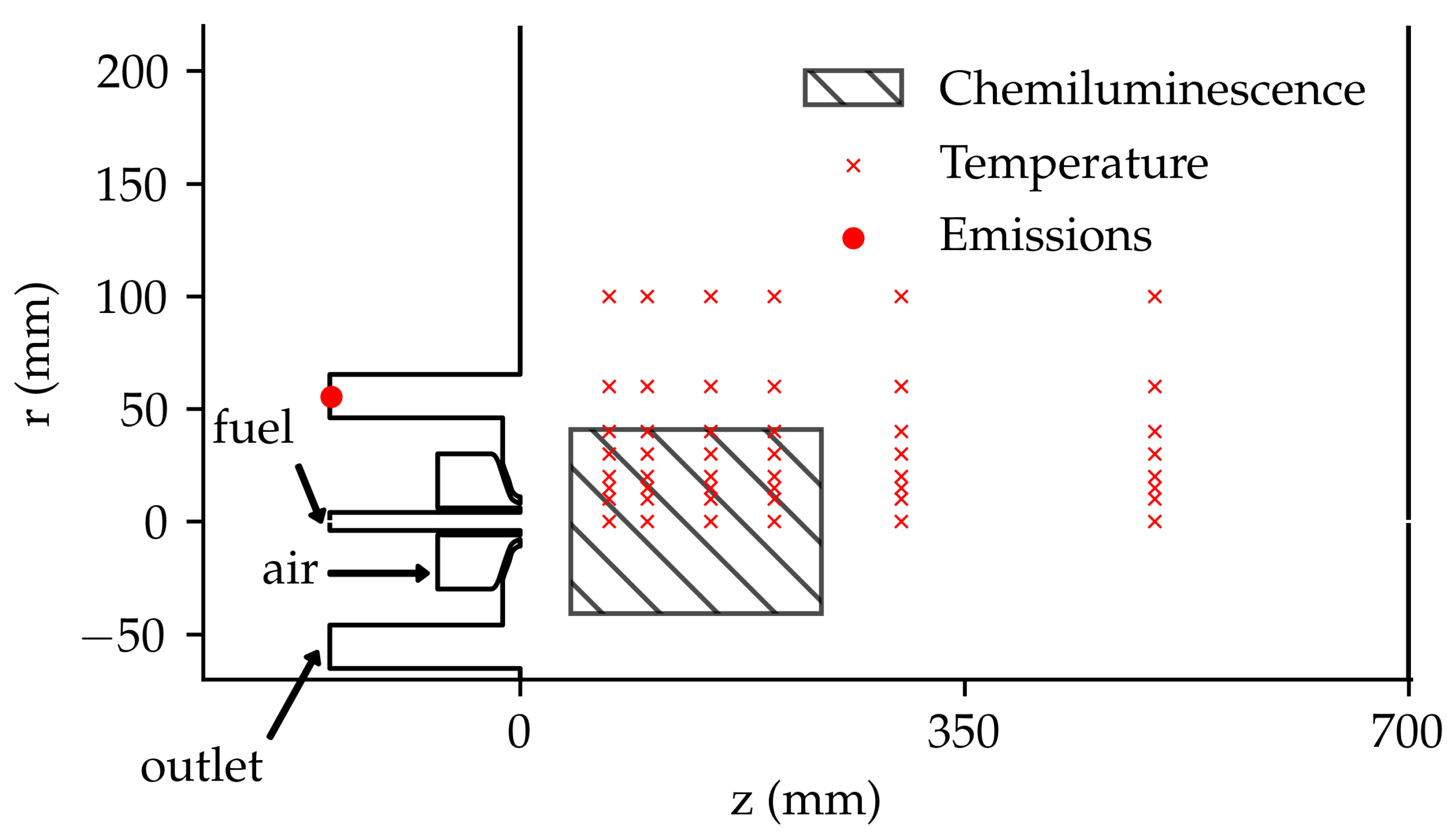
Figure 3 shows the position of the experimental probes inside the furnace. The position of the temperature and the chemiluminescence sensors was chosen to accurately map the reactive region and by considering the design constraints of the set-up. The species concentrations are measured at the outlet of the furnace to check the emissions of pollutants and main combustion products.

The experimental uncertainties for the temperature and the emissions are reported in

Table 1. Experimental uncertainties (95% confidence interval).

T (K)	${\mathit{X}}_{\mathbf{NO}}<200$ (Wet ppmv)	${\mathit{X}}_{\mathbf{NO}}>200$ (Wet ppmv)	${\mathit{X}}_{{\mathbf{NO}}_2}$ (Wet ppmv)	${\mathit{X}}_{\mathbf{CO}}$ (Wet vol. Fraction)	${\mathit{X}}_{{\mathbf{H}}_2\mathbf{O}}$ (Wet vol. Fraction)	${\mathit{X}}_{{\mathbf{CO}}_2}$ (Wet vol. Fraction)	${\mathit{X}}_{{\mathbf{O}}_2}$ (Dry vol. Fraction)
$\pm 20$	$\pm 5.56$	$\pm 19.65$	$\pm 3.93$	$\pm 0.20\%$	$\pm 0.40\%$	$\pm 0.39\%$	$\pm 0.6\%$

.

Operating Conditions

A mixture of ${\mathrm{H}}_2$/${\mathrm{CH}}_4$/$\mathrm{CO}$ has been used as fuel. It is a ${\mathrm{H}}_2$-rich fuel mixture, considered as a surrogate of an industrial Coke Oven Gas (COG) mixture. As in [14], the ${\mathrm{H}}_2$/${\mathrm{CH}}_4$/$\mathrm{CO}$ fuel mixture composition was fixed by considering only the major components of the more complex industrial COG composition. Moreover, the relative ratios of ${\mathrm{H}}_2$, ${\mathrm{CH}}_4$ and $\mathrm{CO}$ correspond to the ones in the fuel source mixture, and they are in accordance with those related to other COG compositions available in literature [15,16,17].

The fuel has been doped with ${\mathrm{C}}_6{\mathrm{H}}_6$ up to 5% (vol.), in order to investigate the effects of aromatic additives in ${\mathrm{H}}_2$-rich fuel mixtures, mainly on $\mathrm{NO}$ emissions and flame radiation, in a semi-industrial furnace.

The compositions of the final six fuel blends tested are provided in

Table 2. Operating conditions of the experimental investigation of ${\mathrm{H}}_2$/${\mathrm{CH}}_4$/$\mathrm{CO}$ fuel mixtures, with different levels of ${\mathrm{C}}_6{\mathrm{H}}_6$(%v/v) doping and equivalence ratios.

Case	${\mathbf{C}}_6{\mathbf{H}}_6$ (%v/v)	$\mathit{\varphi }$	${\mathbf{H}}_2$ (%v/v)	${\mathbf{CH}}_4$ (%v/v)	$\mathbf{CO}$ (%v/v)	LHV ($\mathbf{MJ}/{\mathbf{Nm}}^3$)
1	0	0.80	68.68	25.34	5.98	17.24
2	0.5	0.80	68.34	25.21	5.95	17.86
3	1.12	0.80	67.91	25.06	5.91	18.63
4	2	0.80	67.31	24.83	5.86	19.73
5	3	0.80	66.62	24.58	5.80	20.97
6	5	0.80	65.25	24.07	5.68	23.45
7	0	0.91	68.68	25.34	5.98	17.24
8	0.5	0.91	68.34	25.21	5.95	17.86
9	1.12	0.91	67.91	25.06	5.91	18.63
10	2	0.91	67.31	24.83	5.86	19.73
11	3	0.91	66.62	24.58	5.80	20.97
12	5	0.91	65.25	24.07	5.68	23.45
13	0	1.00	68.68	25.34	5.98	17.24
14	0.5	1.00	68.34	25.21	5.95	17.86
15	1.12	1.00	67.91	25.06	5.91	18.63
16	2	1.00	67.31	24.83	5.86	19.73
17	3	1.00	66.62	24.58	5.80	20.97
18	5	1.00	65.25	24.07	5.68	23.45
19	0	1.05	68.68	25.34	5.98	17.24
20	0.5	1.05	68.34	25.21	5.95	17.86
21	1.12	1.05	67.91	25.06	5.91	18.63
22	2	1.05	67.31	24.83	5.86	19.73
23	3	1.05	66.62	24.58	5.80	20.97
24	5	1.05	65.25	24.07	5.68	23.45
25	0	1.10	68.68	25.34	5.98	17.24
26	0.5	1.10	68.34	25.21	5.95	17.86
27	1.12	1.10	67.91	25.06	5.91	18.63
28	2	1.10	67.31	24.83	5.86	19.73
29	3	1.10	66.62	24.58	5.80	20.97
30	5	1.10	65.25	24.07	5.68	23.45
31	0	1.20	68.68	25.34	5.98	17.24
32	0.5	1.20	68.34	25.21	5.95	17.86
33	1.12	1.20	67.91	25.06	5.91	18.63
34	2	1.20	67.31	24.83	5.86	19.73
35	3	1.20	66.62	24.58	5.80	20.97
36	5	1.20	65.25	24.07	5.68	23.45

, along with the equivalence ratio and the benzene doping.

This was carried out to investigate the effects of aromatics doping of the under-firing ${\mathrm{H}}_2$-fuel mixtures, at both constant and varying air excess.

The thermal input $Q_{\mathrm{th}}$ was kept constant at 20 kW for all the investigated cases. Similarly, the flow rate of the cooling air was kept constant. Moreover, the temperature of the heated fuel pipeline, between the mixing unit and the inlet of the furnace, was controlled to keep a constant inlet fuel temperature of 130 °C, in order to avoid any benzene condensation before the entrance of the furnace.

3. Digital Twin Methodology

As mentioned in Section 1, the goal of this work was to develop a DT capable of predicting simultaneously different types of measurements, such as emissions, temperatures and the chemiluminescence signal.

As a first step, 30 samples of temperature, chemiluminescence and emissions were randomly selected to build the training data. The remaining six samples were used to test the model.

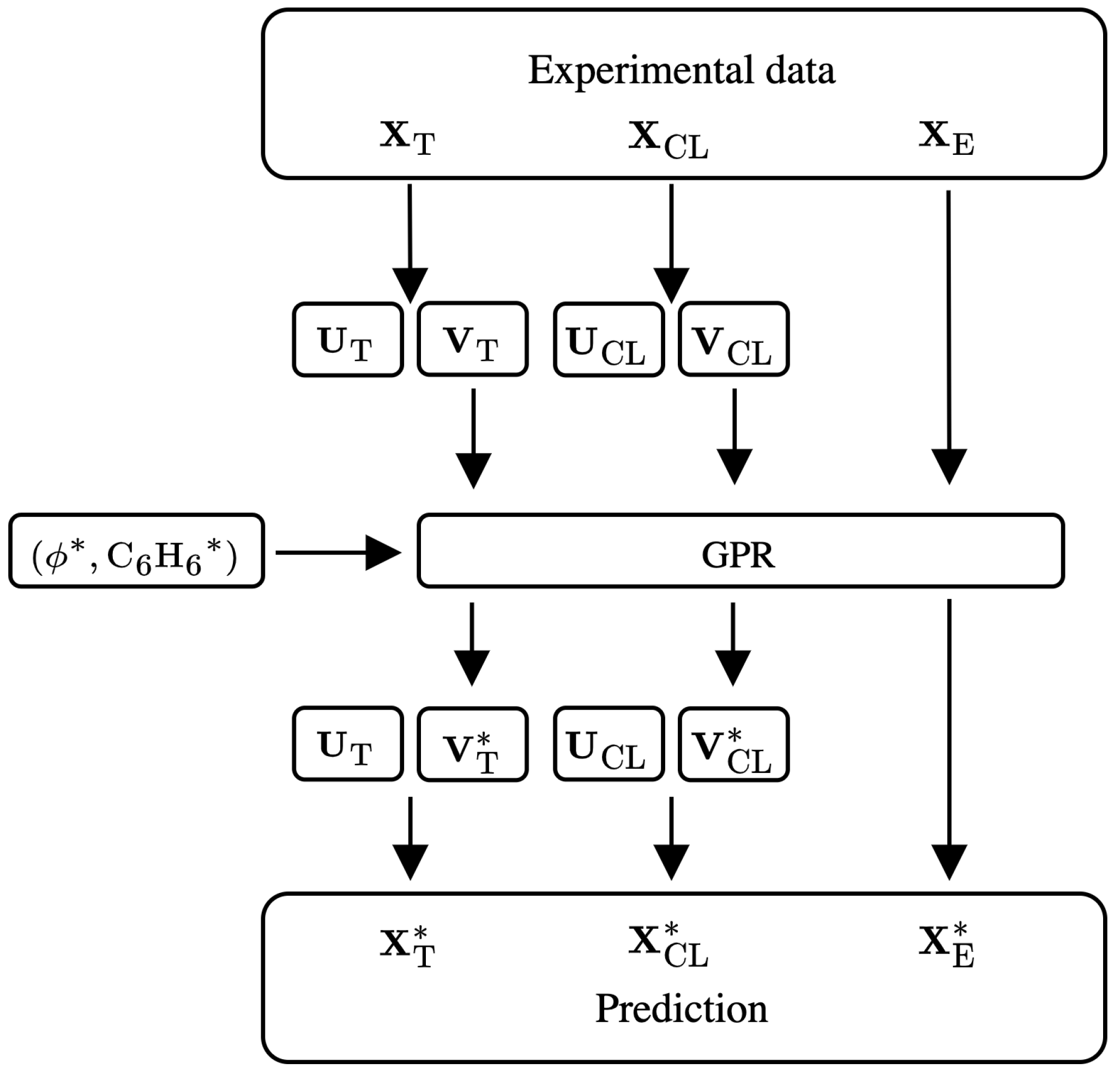
After that, the temperature, chemiluminescence and emissions datasets were arranged into the data matrices ${\mathbf{X}}_{\mathrm{T}}\subset {\mathbb{R}}^{n_{\mathrm{T}},p}$, ${\mathbf{X}}_{\mathrm{CL}}\subset {\mathbb{R}}^{n_{\mathrm{CL}},p}$ and ${\mathbf{X}}_{\mathrm{E}}\subset {\mathbb{R}}^{n_{\mathrm{E}},p}$. Each column vector contains the data for a certain operating condition, and the number of rows depends on the type of measurement. In particular, $n_{\mathrm{T}}=48$, $n_{\mathrm{CL}}=898,560$ and $n_{\mathrm{E}}=6$.

Then, the POD was applied to the data matrices, which were centered and scaled to unitary variance. The POD allows for decomposing the dataset into two parts, of which one is only a function of the spatial coordinates and one is only a function of the parameters:

$${\mathbf{X}}_{\mathrm{T}}(\mathbf{r},\mathit{\theta })={\mathbf{U}}_{\mathrm{T}}\left(\mathbf{r}\right){\mathbf{\Sigma }}_{\mathrm{T}}{\mathbf{V}}_{\mathrm{T}}{\left(\mathit{\theta }\right)}^T,$$

(1)

$${\mathbf{X}}_{\mathrm{CL}}(\mathbf{r},\mathit{\theta })={\mathbf{U}}_{\mathrm{CL}}\left(\mathbf{r}\right){\mathbf{\Sigma }}_{\mathrm{CL}}{\mathbf{V}}_{\mathrm{CL}}{\left(\mathit{\theta }\right)}^T,$$

(2)

where ${\mathbf{U}}_{\mathrm{T}}\subset {\mathbb{R}}^{n_{\mathrm{T}},p}$ and ${\mathbf{U}}_{\mathrm{CL}}\subset {\mathbb{R}}^{n_{\mathrm{CL}},p}$ represent the spatial POD modes while ${\mathbf{V}}_{\mathrm{T}},{\mathbf{V}}_{\mathrm{CL}}\subset {\mathbb{R}}^{p,p}$ contain the parametric coefficients. The diagonal matrices ${\mathbf{\Sigma }}_{\mathrm{T}},{\mathbf{\Sigma }}_{\mathrm{CL}}\subset {\mathbb{R}}^{p,p}$ contain the singular values of the POD modes. The singular values are the square root of the eigenvalues of the covariance matrix $\mathbf{S}=\frac{1}{n-1}{\mathbf{X}}^T\mathbf{X}$, and they reflect the amount of variance retained by each POD mode.

The threshold of $99.9\%$ of explained variance was selected for truncation, resulting in the matrices ${\mathbf{U}}_{\mathrm{T},r}\subset {\mathbb{R}}^{n_{\mathrm{T}},r_{\mathrm{T}}}$, ${\mathbf{U}}_{\mathrm{CL},r}\subset {\mathbb{R}}^{n_{\mathrm{CL}},r_{\mathrm{CL}}}$, ${\mathbf{V}}_{\mathrm{T},r}\subset {\mathbb{R}}^{p,r_{\mathrm{T}}}$ and ${\mathbf{V}}_{\mathrm{CL},r}\subset {\mathbb{R}}^{p,r_{\mathrm{CL}}}$ where $r_{\mathrm{T}}=5$ and $r_{\mathrm{CL}}=8$.

The GPR model was applied to the global data matrix ${\mathbf{X}}_{\mathrm{G}}\subset {\mathbb{R}}^{n,p}$, created by concatenating the matrices ${\mathbf{X}}_{\mathrm{E}}$, ${\mathbf{V}}_{\mathrm{T}}$ and ${\mathbf{V}}_{\mathrm{CL}}$ such that $n=n_{\mathrm{E}}+r_{\mathrm{T}}+r_{\mathrm{CL}}$.

The GPR assumes that, in the classical regression framework,

$$y=f\left(x\right)+ϵ,$$

(3)

the function $f\left(x\right)$ is a sample from a Gaussian process

$$f\left(x\right)\sim GP(m\left(x\right),k(x,x^{\prime })),$$

(4)

where $m\left(x\right)$ and $k(x,x^{\prime })$ are the mean and covariance function of the Gaussian process, which can be thought of as a Gaussian distribution over functions [5]. In this framing, the observed and predicted data become a sample from a multivariate Gaussian distribution:

$$\left[\begin{array}{c}\mathbf{y}\\ {\mathbf{f}}_{*}\end{array}\right]\sim \mathcal{N}\left(\mathbf{0},\left[\begin{array}{cc}\mathbf{K}(\mathbf{X},\mathbf{X})+{\sigma }_n^2\mathbf{I}& \mathbf{K}(\mathbf{X},{\mathbf{X}}_{*})\\ \mathbf{K}({\mathbf{X}}_{*},\mathbf{X})& \mathbf{K}({\mathbf{X}}_{*},{\mathbf{X}}_{*})\end{array}\right]\right),$$

(5)

where $\mathbf{y}$ represents the observed target values, and ${\mathbf{f}}_{*}=f\left({\mathbf{X}}_{*}\right)$ is the prediction in the unexplored part of the design space ${\mathbf{X}}_{*}$. The covariance matrix of the multivariate Gaussian distribution is built using the kernel function $\mathbf{K}$. The prior distribution $p\left(\mathbf{f}\right)$ and the likelihood $p\left(\mathbf{y}\right|\mathbf{f})$ are both assumed to be Gaussian. The prior represents the prior knowledge before considering the data, while the likelihood is the probability of seeing the data given the choice of the model.

By employing Bayes’ theorem, it is possible to calculate the posterior distribution $p\left(\mathbf{f}\right|\mathbf{y})$ given the prior and the likelihood:

$$p\left(\mathbf{f}\right|\mathbf{y})=\frac{p\left(\mathbf{y}\right|\mathbf{f}\left)p\right(\mathbf{f})}{p\left(\mathbf{y}\right)}.$$

(6)

The predicting distribution $p\left({\mathbf{f}}_{*}\right|\mathbf{y})$ is then calculated by marginalizing the likelihood with the posterior distribution:

$$p\left({\mathbf{f}}_{*}\right|\mathbf{y})={\int }_{-\infty }^{+\infty }p\left({\mathbf{f}}_{*}\right|\mathbf{f})p\left(\mathbf{f}\right|\mathbf{y})d\mathbf{f}.$$

(7)

The predicting distribution is again a Gaussian distribution $p\left({\mathbf{f}}_{*}\right|\mathbf{y})=\mathcal{N}({\overline{\mathbf{f}}}_{*},\mathrm{cov}\left({\mathbf{f}}_{*}\right))$ with mean and covariance:

$${\overline{\mathbf{f}}}_{*}={\mathbf{K}}_{*}^T{[\mathbf{K}+{\sigma }_n^2\mathbf{I}]}^{-1}\mathbf{y}$$

(8)

$$\mathrm{cov}\left({\overline{\mathbf{f}}}_{*}\right)={\mathbf{K}}_{**}-{\mathbf{K}}_{*}^T{[\mathbf{K}+{\sigma }_n^2\mathbf{I}]}^{-1}{\mathbf{K}}_{*},$$

(9)

where, for compactness, $\mathbf{K}=\mathbf{K}(\mathbf{X},\mathbf{X})$, ${\mathbf{K}}_{*}=\mathbf{K}(\mathbf{X},{\mathbf{X}}_{*})$ and ${\mathbf{K}}_{**}=\mathbf{K}({\mathbf{X}}_{*},{\mathbf{X}}_{*})$. The model’s hyperparameters, such as the kernel’s length scale and the observations’ noise, are selected by minimizing the negative log marginal likelihood:

$$-\log p\left(\mathbf{y}\right)=\frac{1}{2}{\mathbf{y}}^T{(\mathbf{K}\left(\varphi \right)+{\sigma }_n^2\mathbf{I})}^{-1}\mathbf{y}+\frac{1}{2}\log |\mathbf{K}\left(\varphi \right)+{\sigma }_n^2\mathbf{I}|+\frac{n}{2}\log 2\pi .$$

(10)

Once trained, the GPR model is able to predict the target quantity ${\mathbf{X}}_{\mathrm{G}}^{*}$ in the unexplored part of the design space. In this work, the GPR has been implemented using GPyTorch [18].

The reconstruction of the temperature and chemiluminescence data are carried out by multiplying the respective rows of ${\mathbf{X}}_{\mathrm{G}}^{*}$ times the POD modes ${\mathbf{U}}_{\mathrm{T}}$ and ${\mathbf{U}}_{\mathrm{CL}}$ and the singular values ${\mathbf{\Sigma }}_{\mathrm{T},r}$ and ${\mathbf{\Sigma }}_{\mathrm{CL},r}$:

$${\mathbf{X}}_{\mathrm{E}}^{*}=\mathbf{I}{\mathbf{X}}_G^{*}[1:n_{\mathrm{E}}]$$

(11)

$${\mathbf{X}}_{\mathrm{T}}^{*}={\mathbf{U}}_{\mathrm{T},r}{\mathbf{\Sigma }}_{\mathrm{T},r}{\mathbf{X}}_G^{*T}[n_{\mathrm{E}}:n_{\mathrm{E}}+r_{\mathrm{T}}]$$

(12)

$${\mathbf{X}}_{\mathrm{CL}}^{*}={\mathbf{U}}_{\mathrm{CL},r}{\mathbf{\Sigma }}_{\mathrm{CL},r}{\mathbf{X}}_G^{*T}[n_{\mathrm{E}}+r_{\mathrm{T}}:n],$$

(13)

where the notation $\mathbf{A}[i:j]$ represents the matrix built by considering only the rows of $\mathbf{A}$ between the indices i and j.

The methodology described in this section is summarized in Figure 4.

4. Results

The testing cases randomly selected from the complete dataset are cases 2, 8, 11, 15, 16 and 29. The remaining cases are used to train the model.

The model’s training takes around $10\mathrm{s}$, while the prediction is obtained in around $1\mathrm{s}$.

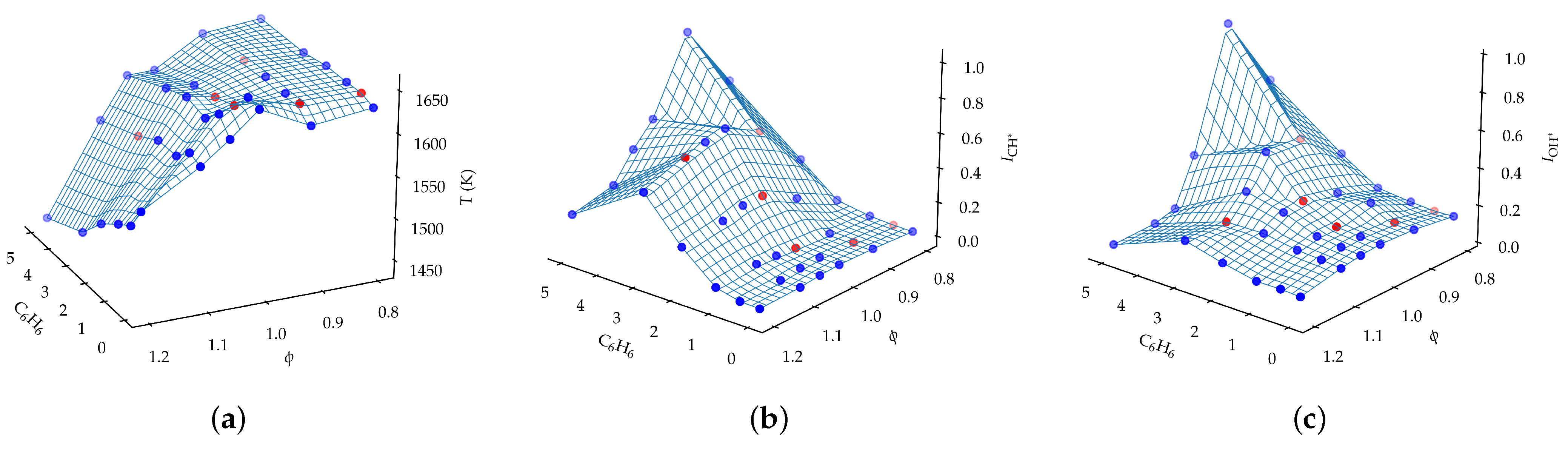
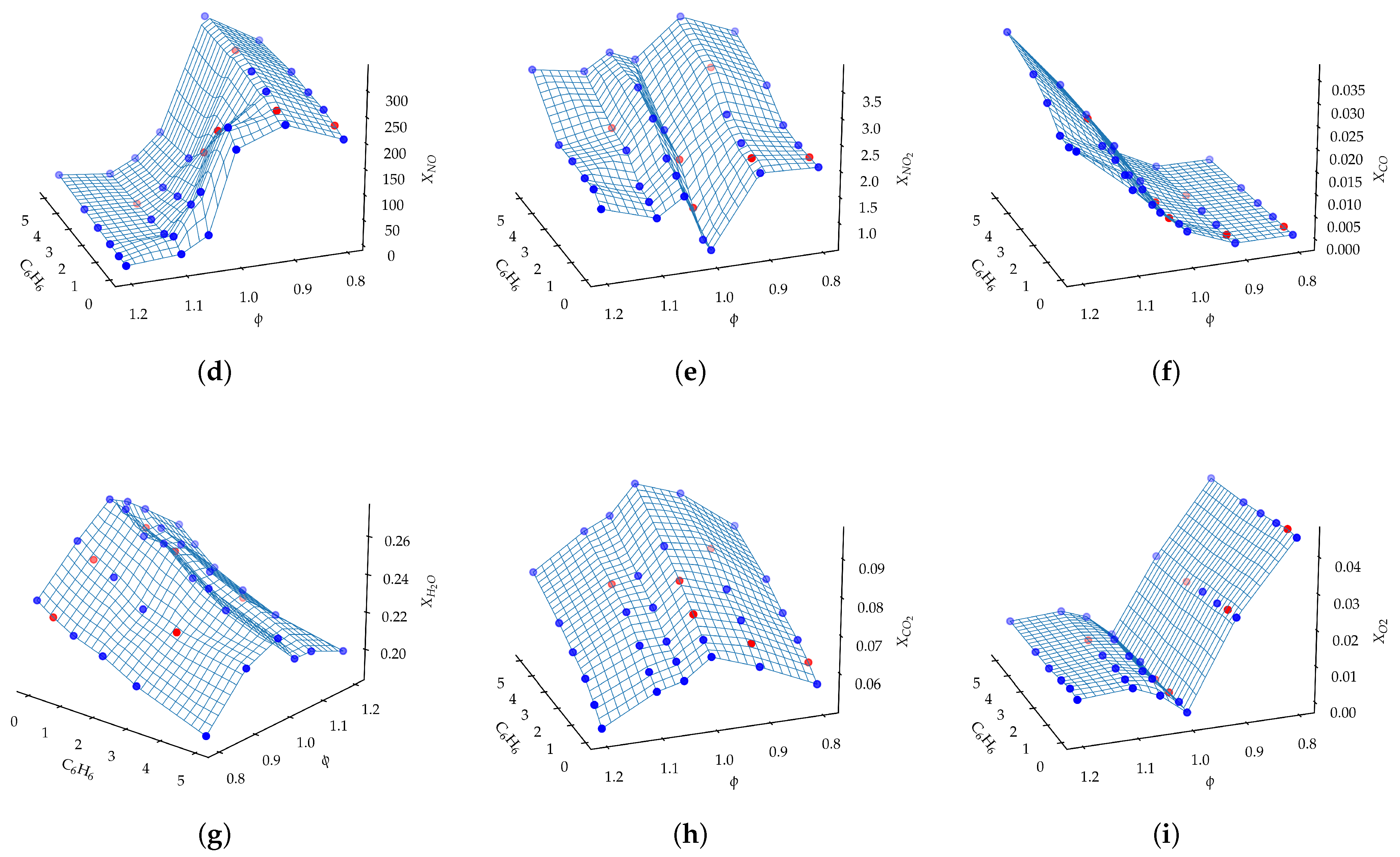
Figure A1 shows the surface response of the scalar quantities of interest as a function of the benzene doping and the equivalence ratio. The scalar quantities selected are the maximum temperature and the normalized sum of the chemiluminescence counts, along with the species concentrations.

The maximum temperature increases slightly with the benzene doping at $\varphi <1.0$, and it reaches the maximum at $\varphi =0.80$ and ${\mathrm{C}}_6{\mathrm{H}}_6=5$. However, by increasing the equivalence ratio above the stoichiometric condition, the maximum temperature drops with the addition of benzene.

The chemiluminescence signal is strongly dependent on both the benzene doping and the equivalence ratio. Similarly to the maximum flame temperature, the intensity of both ${\mathrm{OH}}^{*}$ and ${\mathrm{CH}}^{*}$ chemiluminescence emissions increases with the presence of aromatics in the ${\mathrm{H}}_2$/${\mathrm{CH}}_4$/$\mathrm{CO}$ flames, under lean conditions, showing a distinct maximum at $\varphi =0.91$ and ${\mathrm{C}}_6{\mathrm{H}}_6=5.0\%$, whereas under stoichiometric and rich conditions the chemiluminescence intensity of both ${\mathrm{OH}}^{*}$ and ${\mathrm{CH}}^{*}$ radicals decreases with benzene doping levels higher than 3%.

Figure shows also that the concentration of species such as $\mathrm{NO}$, $\mathrm{CO}$ and ${\mathrm{O}}_2$ depends mainly on the equivalence ratio, while the concentration of ${\mathrm{NO}}_2$, ${\mathrm{H}}_2\mathrm{O}$ and ${\mathrm{CO}}_2$ depends on both the equivalence ratio and the level of benzene doping. The $\mathrm{NO}$ concentration drops when the fuel/air mixture goes from lean to rich, while the opposite happens for the $\mathrm{CO}$ concentration.

Both the ${\mathrm{H}}_2\mathrm{O}$ and the ${\mathrm{CO}}_2$ concentration peaks at $\varphi =1.0$, and it increases with the benzene doping.

Finally, the ${\mathrm{O}}_2$ concentration depends only on the equivalence ratio. In the lean region, the oxygen concentration drops until it reaches the minimum value at stoichiometry. Then, it increases with the equivalence ration in the rich region.

In general, the surface response is nonlinear for all scalar quantities, which justifies the use of a nonlinear regression technique such as the GPR.

The constant mean function was selected to train the GPR model. The kernel function was chosen as the sum of the linear kernel and the radial basis function kernel:

$$K(\mathbf{x},{\mathbf{x}}^{\prime })=v{\mathbf{x}}^T{\mathbf{x}}^{\prime }+\exp \left(-\frac{1}{2}\frac{{(\mathbf{x}-{\mathbf{x}}^{\prime })}^T(\mathbf{x}-{\mathbf{x}}^{\prime })}{{\Theta }^2}\right),$$

(14)

where v and $\Theta$ are the variance and length scale parameters.

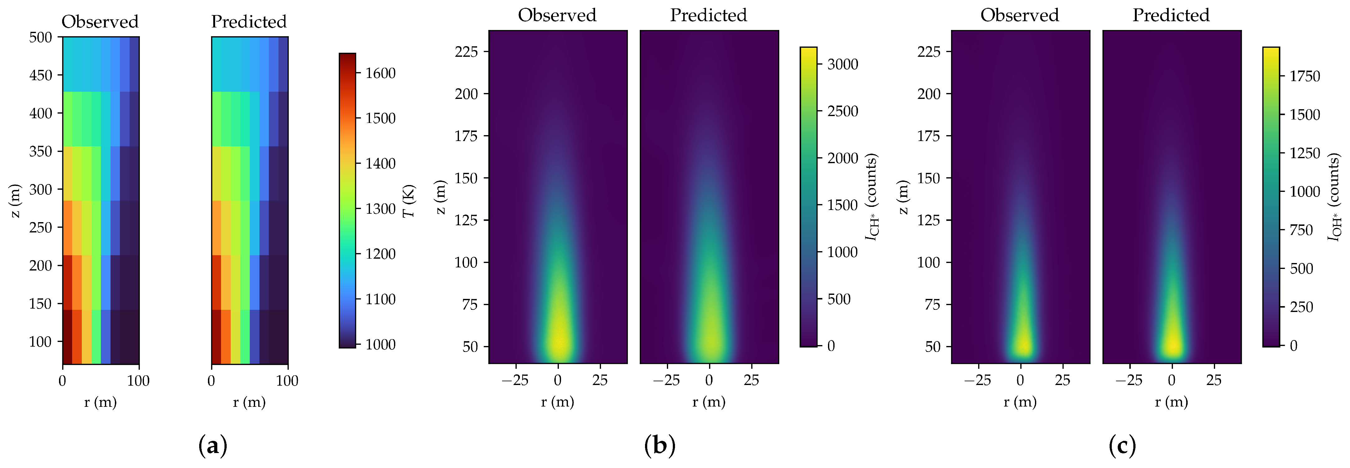
The observed and predicted spatial distribution of the temperature and chemiluminescence signal for case 2 is reported in Figure 5, while the observed and predicted emissions are reported in

Table 3. Observed and predicted species emissions for case 2.

	${\mathit{X}}_{\mathbf{NO}}$ (ppmv)	${\mathit{X}}_{{\mathbf{NO}}_2}$ (ppmv)	${\mathit{X}}_{\mathbf{CO}}$ (Wet vol. Fraction)	${\mathit{X}}_{{\mathbf{H}}_2\mathbf{O}}$ (Wet vol. Fraction)	${\mathit{X}}_{{\mathbf{CO}}_2}$ (Wet vol. Fraction)	${\mathit{X}}_{{\mathbf{O}}_2}$ (Dry vol. Fraction)
Observed	308	$3.25$	0	$0.222$	$0.0828$	$0.0224$
Predicted	304	$3.01$	0	$0.223$	$0.0814$	$0.0231$

.

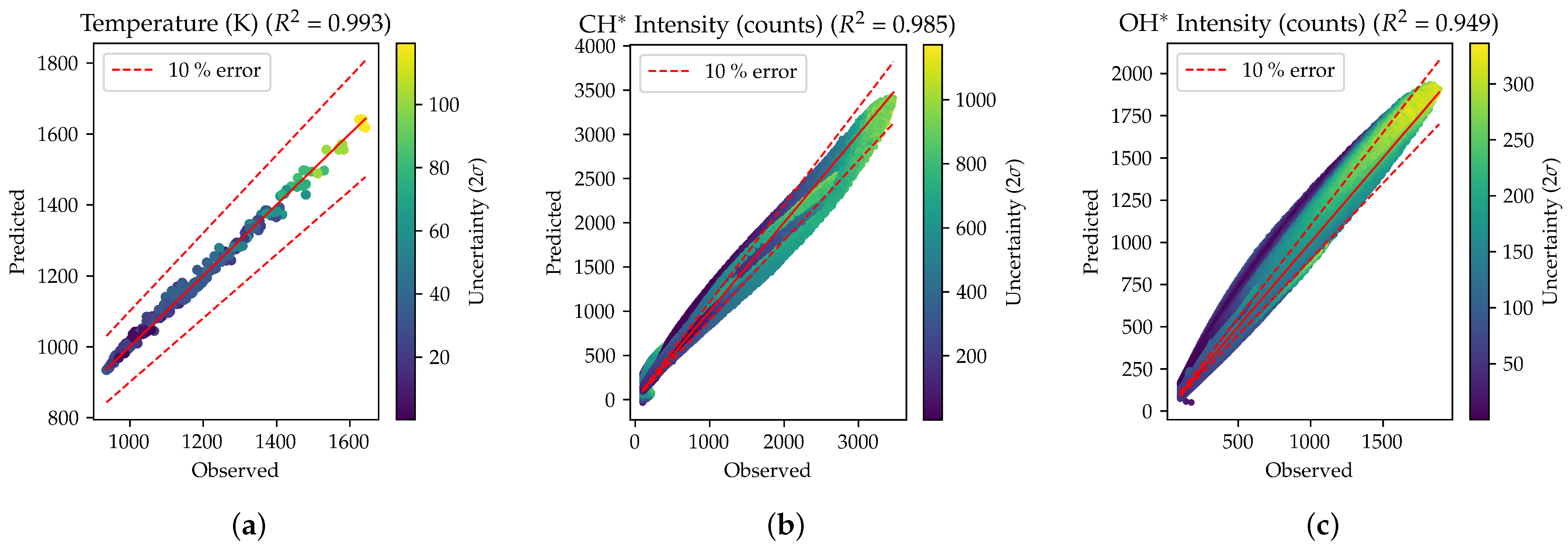
The predictions are generally good, especially for the temperature field. However, the model tends to overpredict the ${\mathrm{OH}}^{*}$ signal, while it underpredicts the ${\mathrm{CH}}^{*}$ signal. This behavior is confirmed for the other testing conditions by looking at Figure 6, which shows the parity plot for all six testing conditions. However, the $R^2$ is well above 0.9 for both ${\mathrm{OH}}^{*}$ and ${\mathrm{CH}}^{*}$. The $R^2$ has been calculated by considering the points with a count greater than 100, to avoid including the non-emitting region.

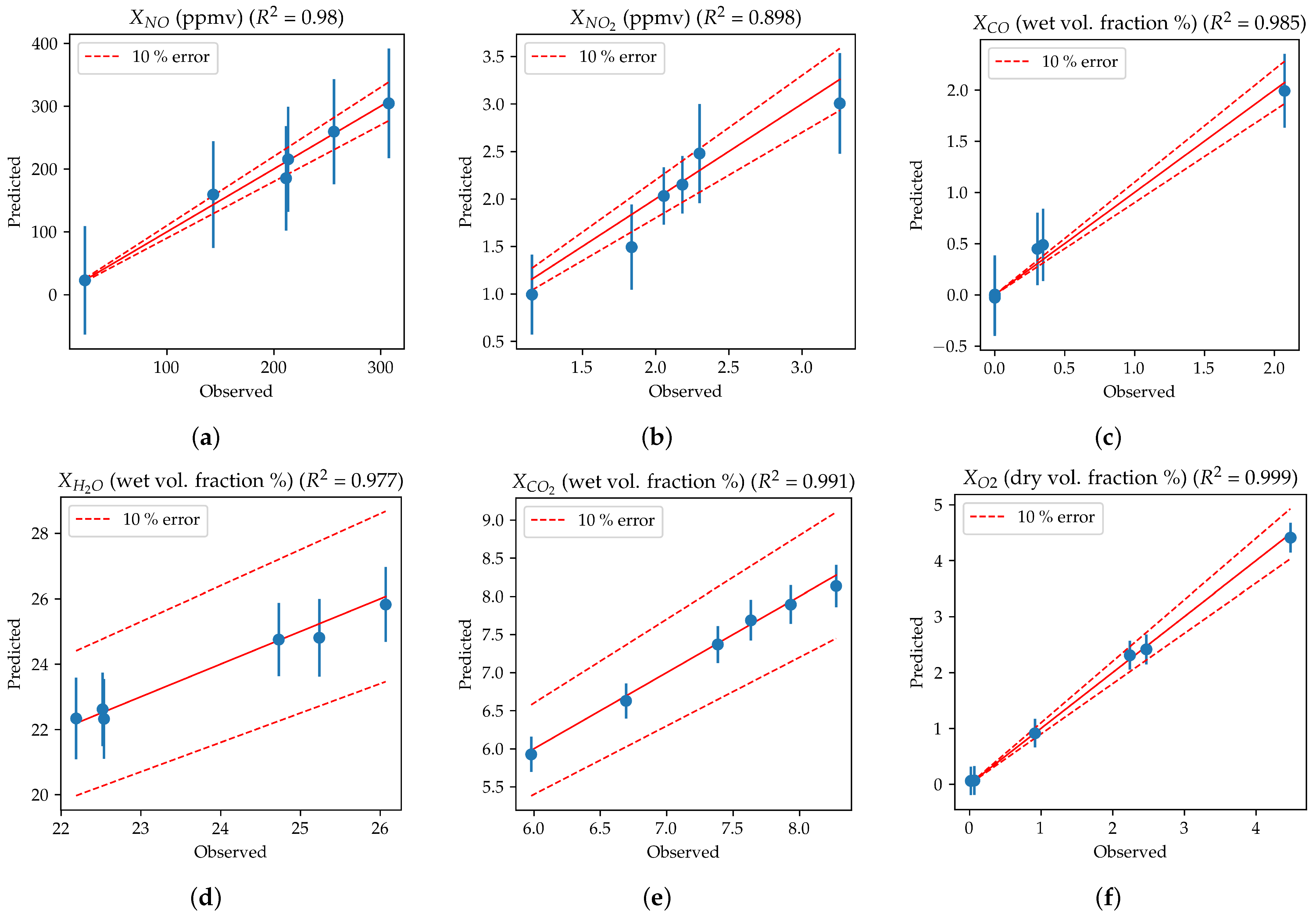
Figure 7 shows the parity plots relative to the prediction of the species emissions. The predictions are good both for minor species, such as $\mathrm{NO}$, and major species, such as ${\mathrm{H}}_2\mathrm{O}$ and ${\mathrm{O}}_2$. The prediction is slightly worse for ${\mathrm{NO}}_2$, which is also associated with the highest relative experimental uncertainty on such a species. This is due to the low ${\mathrm{NO}}_2$ concentrations detected in the exhaust gases with respect to the total instrument error for this species detection (2 ppmv).

If we compare the experimental uncertainty reported in Table 1 with the model’s uncertainty, we can observe that the model’s uncertainty is higher than the experimental uncertainty for measurements such as temperature, $\mathrm{NO}$, $\mathrm{CO}$, ${\mathrm{H}}_2\mathrm{O}$, while it is lower for ${\mathrm{NO}}_2$, ${\mathrm{CO}}_2$ and ${\mathrm{O}}_2$. This suggests that, for those measurements in which the model’s uncertainty is higher than the experimental uncertainty, the number of samples collected was not enough to converge to the experimental uncertainty.

To check the quality of the model’s training, a 6-fold cross-validation was performed on the complete dataset. The 36 samples were randomly divided into six groups (folds), each containing six samples. A GPR model is built for each fold. This model is tested on the data contained in the corresponding fold, while the training data are comprised of all the samples, minus the testing data. The average value of the $R^2$ for each fold is reported in

Table 4. Average and standard deviation of the $R^2$ for the ensemble of folds in the cross-validation algorithm.

	T	${\mathbf{CH}}^{*}$	${\mathbf{OH}}^{*}$	$\mathbf{NO}$	${\mathbf{NO}}_2$	$\mathbf{CO}$	${\mathbf{H}}_2\mathbf{O}$	${\mathbf{CO}}_2$	${\mathbf{O}}_2$
Average	0.988	0.870	0.770	0.966	0.974	0.889	0.945	0.955	0.981
Standard deviation	0.006	0.086	0.168	0.028	0.029	0.094	0.063	0.056	0.012

, along with the standard deviation.

The chemiluminescence signal, ${\mathrm{OH}}^{*}$ in particular, displays the biggest variance in the $R^2$. This is because the chemiluminescence signal has a highly nonlinear behavior as a function of the equivalence ratio and benzene doping, as shown in Figure A1. In addition, the nonlinear behavior is more pronounced on the edge of the operating conditions’ envelope, for ${\mathrm{C}}_6{\mathrm{H}}_6=5\%$. This means that the predictions are accurate when the model is interpolating, i.e., the testing conditions are inside the operating conditions’ envelope. However, when the testing conditions are on the edge of the envelope, the model performs worse because it lacks important information on the behaviour of the chemiluminescence signal as a function of the benzene doping and equivalence ratio.

5. Discussion

The objective of this work was to develop a GPR-based DT capable of predicting the temperature, chemiluminescence and species concentration of a semi-industrial furnace fed with an ${\mathrm{H}}_2$-rich fuel mixture.

To integrate datasets with a vastly different spatial resolution, the POD was applied to the temperature and chemiluminescence signals. This was carried out to decouple the spatial information from the parameter-dependent information.

The GPR was selected as a regression model for its properties, mainly its nonlinearity and the ability to handle sparse datasets.

The predictions show a good level of accuracy, with a $R^2>0.9$ for all the signals except for the ${\mathrm{NO}}_2$ concentration. However, even in this case, the maximum relative error is around 11%.

A 6-fold cross-validation was performed to judge the generalizability of the model. The results show that the prediction of temperature and species concentration is accurate for all combinations of testing conditions. For the prediction of the chemiluminescence signal, the model performs very well in interpolation, while it produces less accurate results in extrapolation. This means that care should be taken in the selection of samples for the model’s training.

In conclusion, the results show that the DT can operate as a real-time surrogate of the corresponding physical object. This opens the possibility of employing the DT for redundant control, state and failure detection or data assimilation if coupled with low-fidelity measurements.