A Surrogate-Assisted Adaptive Bat Algorithm for Large-Scale Economic Dispatch

Abstract

Large-scale grids have gradually become the dominant trend in power systems, which has increased the importance of solving the challenges associated with large-scale economic dispatch (LED). An increase in the number of decision variables enlarges the search-space scale in LED. In addition to increasing the difficulty of solving algorithms, huge amounts of computing resources are consumed. To overcome this problem, we proposed a surrogate-assisted adaptive bat algorithm (GARCBA). On the one hand, to reduce the execution time of LED problems, we proposed a generalized regression neural network surrogate model based on a self-adaptive “minimizing the predictor” sampling strategy, which replaces the original fuel cost functions with a shorter computing time. On the other hand, we also proposed an improved hybrid bat algorithm (RCBA) named GARCBA to execute LED optimization problems. Specifically, we developed an evolutionary state evaluation (ESE) method to increase the performance of the original RCBA. Moreover, we introduced the ESE to analyze the population distribution, fitness, and effective radius of the random black hole in the original RCBA. We achieved a substantial improvement in computational time, accuracy, and convergence when using the GARCBA to solve LED problems, and we demonstrated this method’s effectiveness with three sets of simulations.

1. Introduction

The economic dispatch (ED) problem is a hot spot in power system research and is identified as a nonconvex and nonlinear optimization problem. The purpose of the ED problem is to reasonably distribute load demand to generator units to obtain the minimum cost while meeting the operation and security constraints. The constraints include equality and inequality factors. Among them, it is worth noting that the valve-point effect causes the fuel consumption curve to show pulsation. Additionally, prohibited operation zones (POZs) make the fuel cost functions discontinuous. Other practical constraints, such as ramp rate limits and transmission line losses, should be considered to make ED models more accurate. There have been numerous approaches proposed to resolve the ED problem. On the one hand, some researchers are keen to use traditional mathematical methods, including semidefinite programming [1], dynamic programming [2], $\lambda$-iteration [3], and projection methods [4]. On the other hand, as an important branch of computation intelligence, meta-heuristic algorithms have gained adequate development in solving ED problems, including the generic algorithm (GA) [5], particle swarm optimization (PSO) [6,7], the bat algorithm (BA) [8,9], gray wolf optimizer (GWO) [10], ant colony optimization (ACO) [11], the firefly algorithm (FA) [12], the cuckoo search algorithm (CSA) [13], and the differential evolution algorithm (DE) [14]. In [15], a phasor PSO (PPSO) was applied to solve nonconvex ED problems. Compared with PSO, PPSO had better performance in convergence rate and computing efficiency. In [16], a modified quasi-opposition-based gray wolf optimization algorithm (mQOGWO) was proposed to solve complex constrained optimization problems, including 23 mathematical benchmark functions and three test systems. The mQOGWO algorithm achieved a promising method for solving constrained optimization problems. In [17], the authors proposed a novel honey badger optimization algorithm (HBOA) for ED problems combining heat and power. The simulation results obtained by HBOA were better than other comparison algorithms. In [18], a greedy sine–cosine nonhierarchical gray wolf optimizer (G-SCNHGWO) was employed to solve nonconvex ED problems efficiently. The simulation results demonstrated the superior performance of G-SCNHGWO compared with other state-of-the-art methods. In [19], the authors employed the search and rescue optimization algorithm (SAR) to solve the combined emission and economic dispatch and economic load dispatch. The results proved the superiority of the SAR in the optimal solution for economic load dispatch and combined emission and economic dispatch. In spite of these advances, as society progresses, power systems are becoming larger and cross-regional. As the decision variable dimension increases sharply, the number of fitness evaluations and amount of computation time required for the LED become enormous.

There is a possibility that existing methods will not converge in a timely fashion or will not yield the global optimal result for the LED problem. Al-Betar et al. [20] proposed a new modified $\beta$-hill-climbing local search algorithm for the ED problem, including 3-, 13-, 40-, and 80-unit iterations. When this method was introduced to solve the 40- and 80-unit ED problems, there were at least 900 and 800 fitness evaluations, respectively. The number of assessments is enormous. Chiang [21] proposed an improved genetic algorithm for 20-, 40-, 80-, and 160-unit ED problem simulations. These cases took 80.48, 157.39, 309.41, and 621.30 s, respectively. Ali S. [18] proposed a greedy sine–cosine nonhierarchical gray wolf optimizer to solve ED problems. These four systems include 10, 15, 40, and 140 power generation units, with various assessment times of 250, 220, 350, and 410, respectively. Therefore, traditional mathematical methods and meta-heuristic algorithms that solve LED problems in a straightforward way are considerably time consuming.

Recently, data-driven surrogate-assisted optimization methods have received much attention and achieved many results in large-scale time-consuming optimization problems. The main idea of data-driven surrogate-assisted optimization methods is to build a surrogate model to approximate and replace the exact objective function [22]. The most widely used surrogate models include Kriging models [23,24], artificial neural networks [25,26], radial basis functions [27], support vector machines [28], ensemble models [29], etc. A Kriging-assisted convergence archive and diversity archive evolutionary algorithm was proposed for solving multiobjective expensive problems [23], where an improved Kriging model based on the influential point-insensitive was proposed to approximate an expensive objective function. In [25], compared with the original dropout neural network, which needs to build many network models, a computationally efficient dropout neural network was used to evaluate the fitness value. In [27], radial basis function (RBF) models were applied to replace expensive functions, considerably reducing computing time and resource use.

In addition, as an RBF variant, a generalized regression neural network model (GRNN) was also used for a data-driven approximation of the objective function. Park et al. [30] proposed meta-modeling using GRNN and particle swarm optimization, where GRNN is treated as a global model to approximate the fitness function of the benchmark function. Wang et al. [31] proposed global and local surrogate-assisted differential evolution for expensive constrained optimization problems. GRNN and RBF act as global and local model surrogate-assisted differential evolution algorithms, respectively, where GRNN replaced the objective function to evaluate the vector generated by the differential evolution algorithm. Using GRNN for data-driven surrogate-assisted method has two advantages. First, GRNN only requires a one-time training process. The computational cost and time of training are less than that of RBF. Second, GRNN has only one parameter that needs to be adjusted. This parameter is called the smoothing factor, making the GRNN model insensitive [32]. Although GRNN has been successfully applied to large-scale time-consuming optimization problems, effective sampling criteria are needed to improve the GRNN quality for the fitting error between GRNN and the original objective function.

An effective sampling criterion plays an important role in improving the performance of the surrogate model’s efficiency and fitting error. In [33], a trust-region framework (TRF) for managing surrogate model optimization was first proposed. The framework depends on the gradient information of the expensive function; however, gradient information is difficult to obtain. An improved trust-region model management technology called self-adaptive “minimizing the predictor” (SAMP) was proposed to identity local search space around the optimal solution [34]. Compared with TRF, SAMP uses the different fitness values between two successive iterations to adjust the direction of exploration. SAMP is not only easy to implement but also provides the high-quality sampling points for data needed to improve the quality of GRNN.

An excellent optimization algorithm is useful for the LED problem optimization process. The bat algorithm is widely used in ED problems due to its few parameters and fast convergence [35,36,37,38]. In [39], a modified directional bat algorithm (dBA) was devoted to solving the ED problem with renewable resources. The dBA outperformed the comparison algorithm in terms of convergence speed and computation time. In [40], the authors proposed a novel Cauchy–Gaussian quantum-behaved bat algorithm (CGQBA) to solve the ED problem in various test systems, including 3, 6, 20, 40, 110, and 160 generation units. In [41], the authors proposed a multiobjective hybrid bat algorithm (MHBA) to solve the combined economic/emission dispatch problem. The simulation results from the IEEE 30-, 118-, and 300-bus systems confirmed the superiority of MHBA. In [9], a modified hybrid PSO with BA parameters was presented to find the optimal solution of the ED problem by incorporating renewable energy and thermal sources. Liang et al. [8] proposed a hybrid bat algorithm (RCBA) for ED with random wind power. RCBA was constructed by combining the random black hole model, a chaotic map, and bat algorithm, where random walks for local searches were replaced by the random black hole model, and chaotic maps were applied to substitute some parameters for loudness and pulse emission rate. Compared with the original bat algorithm, RCBAs have the advantages of enhancing the global search ability and effectively avoiding the premature convergence problem. However, the final solution of the RCBA depends heavily on the effective radius ($r_d$) of the random black hole model, and the search space is positively correlated with $r_d$. Importantly, $r_d$ is set as a piecewise parameter by the author based on the search space variation (from large to small) and experience, which has a considerable effect on convergence and accuracy. Furthermore, Zhan et al. [42] proposed an adaptive PSO. A real-time evolutionary state estimation method (ESE) based on population distribution and particle fitness was performed to identify one of four defined evolutionary states in each generation. Inertia weights, acceleration coefficients, and other algorithmic parameters were automatically controlled at runtime to enhance search efficiency.

Although the surrogate model technique and LED problem have been actively studied, there are few data-driven surrogate-assisted optimization algorithms to solve the LED problem. To improve the quality of the surrogate model and obtain the better final solution for the LED problem, a high-quality hybrid optimization algorithm is urgently needed. Motivated by the above analysis, we proposed a data-driven surrogate-assisted adaptive hybrid bat algorithm for the LED problem. Our proposed method consists of two parts: (1) a novel GRNN surrogate model based on the SAMP sampling strategy; (2) an adaptive hybrid bat algorithm.

The main contributions of our paper are summarized as follows:

(1)

We proposed an improved GRNN based on the SAMP sampling strategy for replacing the original objective function in optimization. First, we used GRNN to evaluate the fitness, which is constructed from the population that meets the constraint conditions and is randomly generated. The promising points $x_p$ randomly sampled from the SAMP search space are 10 percent of the number of the population in each iteration. Then, $x_p$ are taken to the database, and GRNN is finally updated according the database in every five generations;

(2)

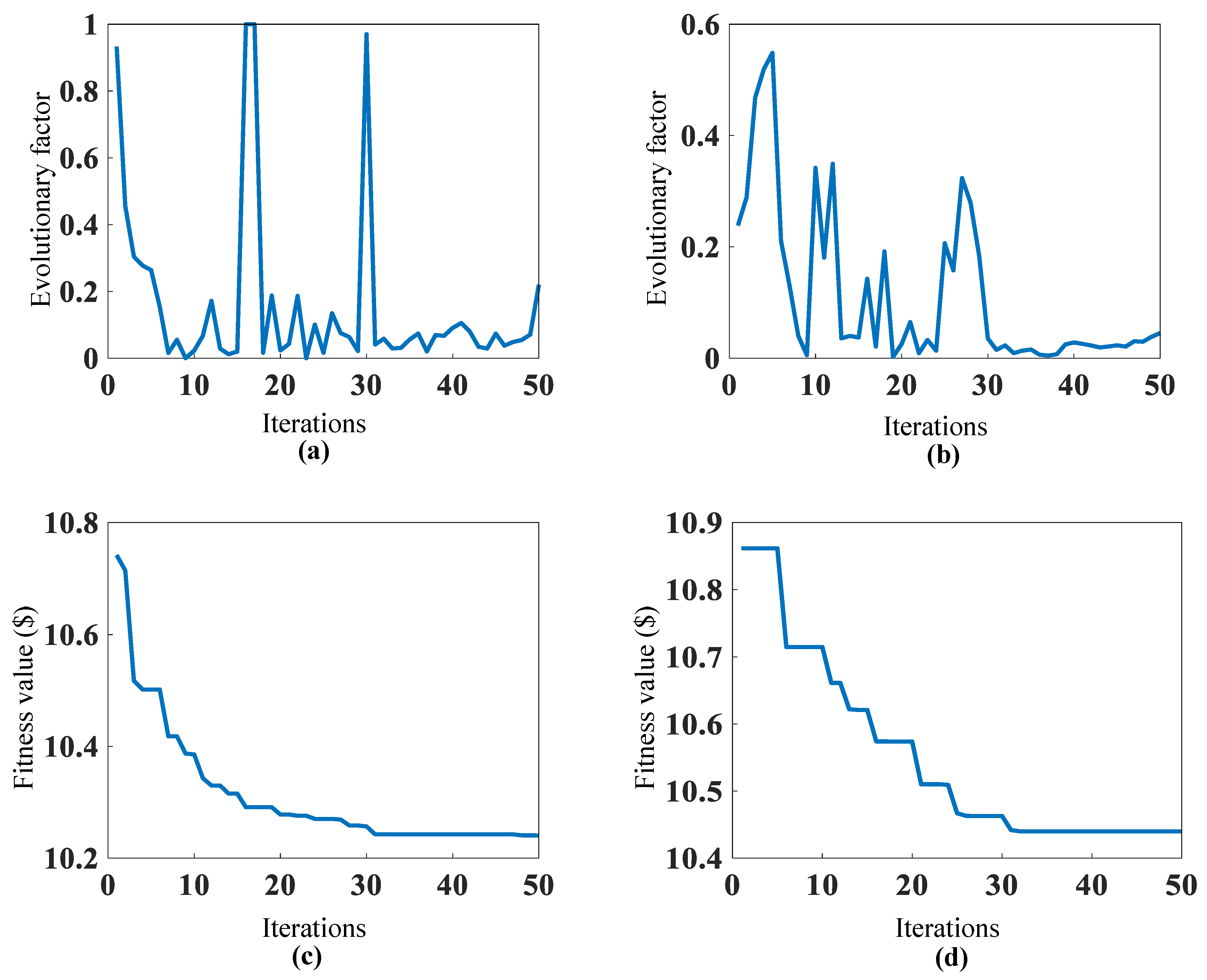
We proposed an adaptive bat algorithm to perform LED-problem optimization. First, by revealing the essence of $r_d$ in RCBA, we developed the ESE method to evaluate the relationship between the population distribution, fitness value, and $r_d$ of RCBA. ESE can improve the reliability of RCBA without increasing the algorithm’s complexity. Second, inspired by the principle of the evolutionary factor in ESE, we proposed an average evolutionary factor method to adaptively update $r_d$. Based on this, an adaptive bat algorithm was proposed, which eliminates the irrationality of the previous piecewise setting.

The rest of this paper is organized as follows. Section 2 describes the economic dispatch problem. Section 3 describes the related work. The proposed algorithm and surrogate are introduced in Section 4. Section 5 presents the experimental studies on the IEEE 118- and 300-bus systems, as well as the IEEE 40-unit test system. Finally, Section 6 concludes this paper and provides future research directions.

2. Problem Formulation

This section describes LED problems and aims to minimize the cost, which is subject to constraints. The LED problem is to increase decision variables and search space on the basis of the ED problem. Specifically, constraints are introduced to the objective function. The object is to minimize the fuel cost functions of thermal units with or without valve points, which are given

$$\min F_1=\sum _{j=1}^{N_g}{F}_j\left(P_j\right)=\sum _{j=1}^{N_g}\left({\alpha }_j{P}_j^2+{\beta }_j{P}_j+{\gamma }_j\right),$$

(1)

where $F_j\left(P_j\right)$ is the cost function of the jth generator (USD/h); $N_g$ is the number of generators; $P_j$ is the active output of the jth generator (MW); and ${\alpha }_j,{\beta }_j,{\gamma }_j$ are the cost coefficients of the jth generator. In the practical ED problem, when the intake valve is opened, the drawing effect will cause the fuel cost to rise sharply in a short time, finally causing the cost function to have many non-differentiable points [43]. Therefore, if the valve-point effects are considered, the fuel cost function is expressed as follows:

$$\begin{array}{cc}\hfill \min F_2& =\sum _{j=1}^{N_g}{F}_j\left(P_j\right)\hfill \\ \hfill & =\sum _{j=1}^{N_g}\left[{\alpha }_j{P}_j^2+{\beta }_j{P}_j+{\gamma }_j+\left|e_{j}sin\left(d_j(P_j^{min}-P_j)\right)\right|\right],\hfill \end{array}$$

(2)

where $e_j$ and $d_j$ are the valve-point coefficients of the jth generator; $P_j^{min}$ is the minimum active output of the jth generator (MW).

To describe the economic dispatch problem more practically, we considered reactive power limits, voltage magnitude constraints, line flow constraints, prohibited operation zones, ramp rate limits, and valve-point effects [41].

• Generation capacity constraints: the real active and reactive outputs of generators should be limited between their minimum and maximum, which means that generators should satisfy the following inequality constraint:

  $$P_j^{min}\le P_j\le P_j^{max},Q_j^{min}\le Q_j\le Q_j^{max},$$

  (3)

  where $P_j^{min}$ and $P_j^{max}$ are the minimum and maximum active power outputs of the jth generator, respectively; $Q_j^{min}$ and $Q_j^{max}$ are the minimum and maximum reactive power outputs of the jth generator, respectively.
• Power balance constraint: the whole active power output should include the total load demand $P_d$ and total transmission line loss $P_l$.

  $$\sum _{j=1}^{N_g}{P}_j=P_d+P_l,$$

  (4)
  The $P_l$ is calculated by [44]:

  $$P_j-P_{dj}-V_j\sum _{k=1}^{N_b}{V}_k(G_{jk}cos{\theta }_{jk}+B_{jk}sin{\theta }_{jk})=0,$$

  (5)

  $$Q_j-Q_{dj}-V_j\sum _{k=1}^{N_b}{V}_k(G_{jk}sin{\theta }_{jk}-B_{jk}cos{\theta }_{jk})=0,$$

  (6)

  where $P_j$ and $Q_j$ are the active and reactive powers of the jth bus, respectively; $P_{dj}$ and $Q_{dj}$ are the active and reactive power load needs of the jth bus, respectively; $G_{jk}$ and $B_{jk}$ are the transfer conductance and susceptance of the jth bus to kth bus, respectively; $V_j$ and $V_k$ are the voltage magnitudes of the jth bus and kth bus, respectively, (V); $N_b$ is the number of buses; and ${\theta }_{jk}$ are the voltage angles of the jth bus to kth bus, respectively. The real $P_l$ is calculated after obtaining $V_j$, $V_k$, and ${\theta }_{jk}$ by:

  $$P_l=\sum _{m=1}^{N_{\mathrm{line}}}{G}_m[V_j^2+V_k^2-2V_j{V}_{k}cos{\theta }_{jk}],$$

  (7)

  where $G_m$ is the conductance of the mth line connecting buses j and k; $N_{\mathrm{line}}$ is the number of transmission lines.
• Voltage magnitude constraints: the voltage magnitude should be limited from the lower to upper bounds for secure operation.

  $$V_j^{min}\le V_j\le V_j^{max},j=1,\dots ,N_b.$$

  (8)
• Line flow constraints: the security constraint of the transmission line is limited by

  $$S_j\le S_j^{max},j=1,\dots ,N_{\mathrm{line}},$$

  (9)

  where $S_j$ and $S_j^{max}$ are the line flows of the jth line and jth line, respectively.
• Ramp rate limits: the active output of the generators cannot be suddenly increased or decreased. Thus, it is limited by:

  $$\left\{\begin{array}{cc}{P}_j-P_j^0\hfill & \le U{R}_j,\hfill \\ P_j^0-P_j\hfill & \le D{R}_j,\hfill \end{array}\right.$$

  (10)

  where $P_j^0$, $U{R}_j$, and $D{R}_j$ are the previous active output power and the up- and down-ramp limits of the jth generator, respectively;
• Prohibited operating zones: the thermal generator’s steam valve operation or bearing vibration makes the cost function discontinuous. Therefore, prohibited operating zones are considered as below:

  $$\left\{\begin{array}{c}{P}_j^{min}\le P_j\le P_{j,1}^l,\hfill \\ P_{j,k-1}^u\le P_j\le P_{j,k}^l,k=2,\dots ,z,j=1,2\dots ,N_g\hfill \\ P_{j,z}^u\le P_j\le P_j^{max},\hfill \end{array}\right.$$

  (11)

  where z is the number of prohibited operation zones of the jth generator; $P_{j,z}^u$ and $P_{j,z}^l$ are the upper and lower active power outputs of the zth prohibited operation zones for the jth thermal unit.

3. Related Technology

This section is devoted to introducing the original hybrid bat algorithm RCBA, evolutionary state evaluation method, general regression neural network, and self-adaptive “minimizing the predictor” strategy.

3.1. Original Hybrid Bat Algorithm RCBA

RCBA [8] is an improved hybrid bat algorithm, which was proposed to solve ED with random wind power. The main idea of RCBA is to integrate the random black hole model and chaotic maps with the bat algorithm, greatly increasing the global search ability, enlarging the exploitation area, and accelerating convergence speed during the search. To enhance convergence for solving ED problems, the authors adopted the random black hole model to replace the random walk of the bat algorithm, which shows high performance for its convergence and search abilities. Our use method of the random black hole model is stated as follows:

$$f_i=f_{min}+(f_{max}-f_{min})\beta ,$$

(12)

$$V_i^{t+1}=V_i^t+(X_i^t-X_g^t)f_i,$$

(13)

$$\begin{array}{c}\hfill \left\{\begin{array}{c}{X}_i^{t+1}\left(m\right)=X_g^t\left(m\right)+r_d\ast \sigma ,l\le p,\hfill \\ X_i^{t+1}=X_i^t+V_i^{t+1},l>p,\hfill \end{array}\right.\end{array}$$

(14)

where $f_{max}$ and $f_{min}$ represent the maximum and minimum frequencies, respectively; $\beta$ is a random number distributed in the range (0,1); $V_i^t$ is the bat velocity at the tth iteration; $X_g^t\left(m\right)$ is the current best position of each single dimension m at the tth iteration; $X_i^{t+1}\left(m\right)$ is the current position of each single dimension m at the $t+1$th iteration; $r_d$ is the effective radius of the random black hole model, which is set as a piecewise parameter; $\sigma$ obeys uniform distribution in [−1,1]; l is a random number that takes a value between 0 and 1; and p is the threshold of the random black hole model—a constant.

Accordingly, loudness $A_i$ and pulse emission rate $r_i$ are updated by Equations (15) and (16), respectively.

$$\begin{array}{ccc}\hfill A_i^{t+1}& =& \left\{\begin{array}{c}{A}_i^t/0.7,if{A}_i^t<0.7,\hfill \\ 10(1-A_i^t)/3,if{A}_i^t\ge 0.7,\hfill \end{array}\right.\hfill \end{array}$$

(15)

$$\begin{array}{ccc}\hfill r_i^{t+1}& =& r_i^t+0.2-((0.5/\left(2\pi \right))\times sin(2\pi \times r_i^t))mod1,\hfill \end{array}$$

(16)

The update steps of RCBA are as follows:

(1)

Initialize bat population, velocity, frequency, loudness, and pulse emission rate;

(2)

Obtain fitness values by Equation (1) or (2);

(3)

Generate p, $\sigma$, and new solutions by frequency, speed, position, and Equations (12)–(14);

(4)

Update $X_i^{t+1}\left(m\right)$ according to Equation (14) if $l\le p$;

(5)

Generate new fitness;

(6)

Update new fitness and position if the solution improves, or update if not;

(7)

Update the best solution, loudness, and pulse emission rate updated by Equations (15) and (16);

(8)

Repeat steps 3 to 7 until the stopping criterion is satisfied.

The effect radius $r_d$ of the random black hole model is a piecewise parameter, which has an important effect on convergence and global search ability. If $r_d$ is considerably large, the final solution will be away from the global best solution. In contrast, when $r_d$ is considerably small, the ability to enlarge the search area may be reduced.

3.2. Evolutionary State Evaluation Method

In the optimization process, it can be expected that the population distribution will cluster around the global optimum from the initial uniform random distribution to the later stage. First, we proposed the ESE method to calculate the average distance of each particle to all other particles [42]. The population distribution state is reflected through the average distance. The average distance of the global optimal particle to all other particles tends to be the smallest, because all other particles tend to surround the global optimal. At this point, the evolutionary state can be judged as a convergent state. In contrast, when the average distance is the largest, the global optimum is far from all other particles in the jumping-out state. Detailed steps are introduced as follows:

(1)

Average distance is calculated by the Euclidean metric from the particle i to all the other particles, where $N_p$ is the population size and D is the number of dimensions, respectively.

$$d_{ip}=\frac{1}{N-1}\sum _{j=1,j\ne i}^{N_p}\sqrt{\sum _{k=1}^D{(x_i^k-x_j^k)}^2};$$

(17)

(2)

Evolutionary factor is denoted as the variation in the average distance of the global optimal particle during the optimization process, where $d_{\ast }$ is the average distance of the global optimal particle. In addition, the maximum and minimum average distances of all $d_i$ are defined as $d_{max}$ and $d_{min}$, respectively.

$$f_{ese}=\frac{d_{\ast }-d_{min}}{d_{max}-d_{min}}\in [0,1];$$

(18)

(3)

According to the concept of fuzzy classification, $f_{ese}$ is classified into four sets, namely $S_1$, $S_2$, $S_3$, and $S_4$, which represent the states of exploration, exploitation, convergence, and jumping out, respectively.

3.3. General Regression Neural Network

The GRNN, which can approximate any regression surface in theory, was proposed by Specht [45]. In this paper, we used the GRNN to approximate cost function (1) or (2) in the LED problem. Compared with other neural networks, such as the back propagation neural network, the GRNN requires only one training process. Therefore, the GRNN is suitable for solving time-consuming LED problems. Assuming that x and y are two random variables, their joint probability density is $f(x,y)$, and the regression of y relative to $x_0$ is given by

$$E\left(y\mid x_0\right)=\left(x_0\right)=\frac{{\int }_{-\infty }^{0}yf\left(x_0,y\right)dy}{{\int }_{-\infty }^{0}f\left(x_0,y\right)dy},$$

(19)

where $y\left(x_0\right)$ is the predicted output of y given the input $x_0$. A Parzen sub-parameter estimation of the density function $f(x_0,y)$ can be obtained from the sample dataset ${(x_i,y_i)}_{i=1}^n$ [46]:

$$f\left(x_0,y\right)=\frac{1}{n{\left(2\pi \right)}^{\frac{p+1}{2}}{\sigma }^{p+1}}\sum _{i=1}^n{\mathrm{e}}^{-d\left(x_0,x_i\right)}{\mathrm{e}}^{-d\left(x_0,x_i\right)},$$

(20)

$$\begin{array}{c}d\left(x_0,x_i\right)=\sum _{j=1}^p{\left[\left(x_{0j}-x_{ij}\right)/\sigma \right]}^2,\\ d\left(y,y_i\right)={\left[y-y_i\right]}^2,\end{array}$$

(21)

where n is the number of sample points; p is the dimension of random variables x; $\sigma$ is called the smoothing factor, which is actually the standard deviation of the Gaussian function. By combining Equations (19)–(21), $y\left(x_0\right)$ is calculated by:

$$E\left(y\mid x_0\right)=\frac{{\sum }_{i=1}^{n}y{\mathrm{e}}^{-d\left(y_0,y_i\right)}}{{\sum }_{i=1}^n{\mathrm{e}}^{-d\left(x_0,x_i\right)}},$$

(22)

Obviously, when given input $x_0$, the predicted result is $E\left(y\mid x_0\right)$. It should be noted that the value of the smoothing factor has a large impact on network performance.

3.4. A Self-Adaptive “Minimizing the Predictor” Strategy

To make the Kriging model gradually approximate the real objective function through continuous sampling, a self-adaptive “minimizing the predictor” (SAMP) strategy [34] is presented by Dong. Specifically, by continuously sampling the local optimal solution of the minimization problem, the surrogate model continuously approximates the true objective function. Because the surrogate model has a better approximation effect near the local optimum point $x_0$, a search radius is required to determine the next sample point $x_1$. The initial search radius $r_0$ may be set by a specific problem. The next sampling point can be sampled by the surrogate model in the interval $x_0\pm r_0$. The trust-region factor r is obtained by:

$$r=\frac{f\left(x_{j-1}\right)-f\left(x_j\right)}{f\left(x_{j-1}\right)-\widehat{y}\left(x_j\right)},$$

(23)

where $f\left(x_{j-1}\right)$ and $f\left(x_j\right)$ are the real objective function values at sample points $x_{j-1}$ and $x_j$, respectively; $\widehat{y}\left(x_j\right)$ is the function value computed by the surrogate model at the sampling point $x_j$. The next search radius ${\sigma }_1$ is calculated by:

$${\delta }_j=\left\{\begin{array}{cc}{c}_1∥x_j-x_{j-1}∥\hfill & \mathrm{if}r<r_1\\ min\left\{c_2∥x_j-x_{j-1}∥,\Delta \right\}\hfill & \mathrm{if}r>r_2\\ ∥x_j-x_{j-1}∥\hfill & \mathrm{otherwise}\end{array}\right.$$

(24)

where $c_1$ and $c_2$ represent the contraction and expansion degree coefficients of the new search area (trust region), respectively. The parameters $r_1$ and $r_2$ determine the boundaries of contraction and expansion, respectively. If the model performance is low, r will be less than $r_1$ and the trust region will shrink. Conversely, if the model performance is high, r will be more than $r_1$ and the trust region will expand.

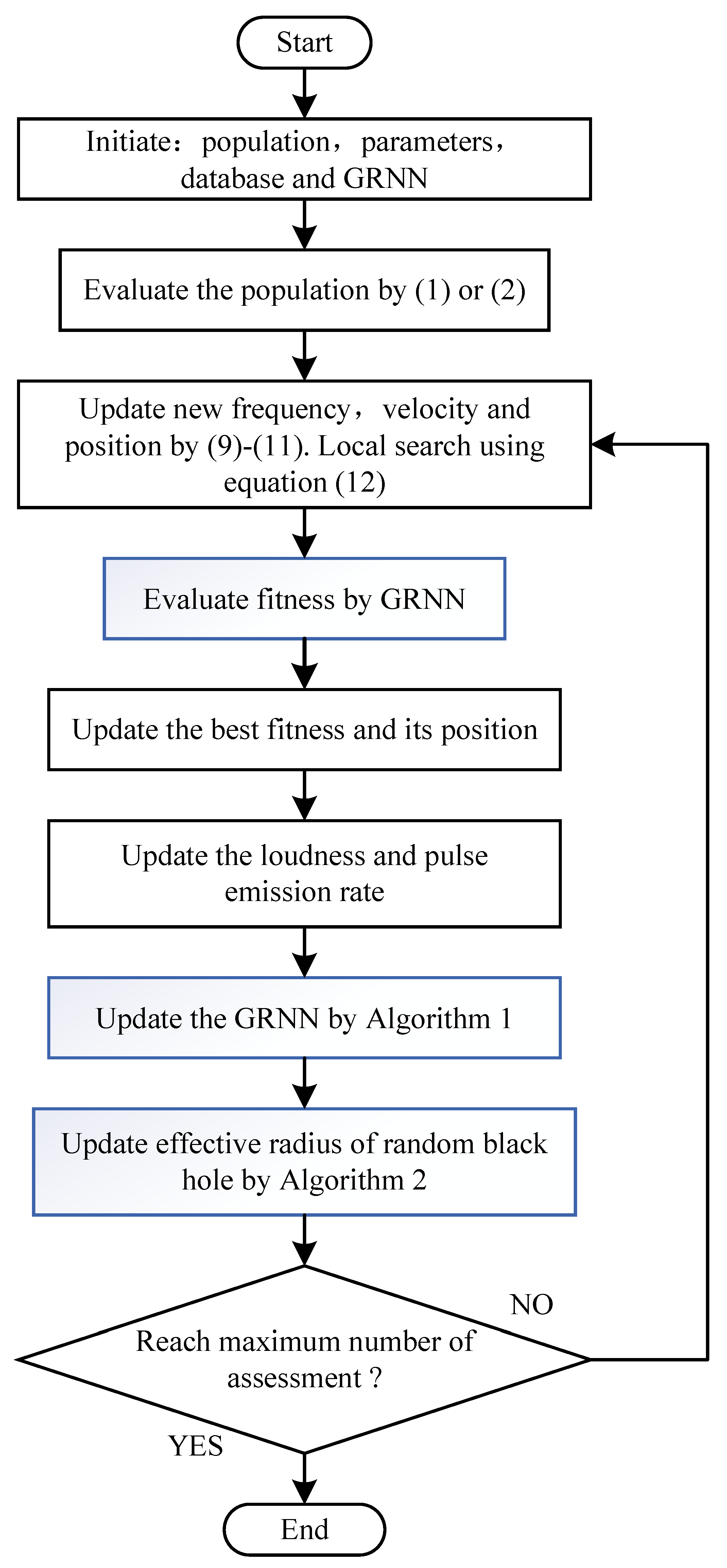
4. Proposed Method (GARCBA)

In our work, we proposed an improved general regression neural network surrogate-assisted adaptive bat algorithm (GARCBA) for LED problems. Figure 1 shows a flowchart of our method. Unlike the existing algorithms for ED, the GARCBA consists of two parts: a surrogate model and an algorithm. In the GARCBA, the GRNN is employed as the surrogate model to approximate the objective function, which can greatly reduce computational time. For a accurate GRNN, we adopted the SAMP sampling strategy for promising points to join the database in every generation. The GRNN is updated every five generations. To obtain better fitness for enhancing the GRNN’s quality and further solving the LED problem, we proposed an adaptive bat algorithm. First, we developed ESE to estimate the relationship of the population distribution, fitness value, and $r_d$ of the RCBA. Second, we proposed an adaptively updated $r_d$ of the random black hole method to remove the irrationality of the segmented setting of $r_d$.

(1)

Initialization: The initial population is generated by pseudo-random number generators when meeting the constraints. The database is built through the initial population and used to build a GRNN for replacing objective function (1) or (2). In addition, the initial parameters include the maximum frequencies $f_{max}$, minimum frequencies $f_{min}$, velocity $v_0$, loudness $A_0$, pulse emission rate $r_0$, population size $r_0$, and system load.

(2)

Evaluate the population by exact function: If the valve-point effect is considered, Equation (2) is used to evaluate the initial population; otherwise Equation (1) is used to evaluate the initial population.

(3)

Update bat frequency, velocity, position, and local search by random black hole model: The frequency, velocity, and position are updated by Equations (12)–(14). The random black hole model is used for local search, which not only enhances the search ability but also increases convergence. Note that $r_d$ is set as a piecewise parameter that seriously effects the algorithm’s performance.

(4)

Evaluate the fitness by the GRNN: The GRNN is used to replace the real objective function for evaluating the fitness, which can greatly reduce the computational time.

(5)

Obtain the current best fitness and its position: The best fitness value and the corresponding bat position are predicted by the GRNN at each iteration, where the best fitness value is used for the SAMP sampling strategy of the GRNN, and the best bat position is used in the random black hole model (see Equation (14)).

(6)

Update the loudness and pulse emission rate: Finally, the loudness and pulse emission rate are updated according to the chaotic map (see Equations (15) and (16)).

(7)

Update GRNN: Within the SAMP sampling strategy, the promising points of 10 percent of the population are randomly generated and evaluated by the real cost function. Then, the promising points are taken in the database. Finally, the GRNN is retrained using the database every five generations.

(8)

Estimate the relationship between evolutionary factor and fitness by ESE and adaptively update the effective radius $r_d$ of the random black hole: The ESE is introduced to clearly show the state of the bat position and fitness in every generation. According to the ESE, the average evolutionary factor is proposed to adaptively update $r_d$.

(9)

Repeat steps 3 to 7 until the stopping criterion is satisfied.

4.1. An Improved GRNN Base on SAMP Sampling Strategy

As noted in Section 3.3, the GRNN training process is only needed once, which can greatly reduce computational time. In addition, the GRNN parameter is only a smoothing factor, which can reduce the GRNN complexity. However, the aforementioned GRNN is trained by the initial data, which causes an increasing error between the surrogate model and real objective function. To prevent the algorithm from convergence to a false optimum, we considered that the SAMP strategy samples new promising points, which can increase GRNN accuracy to approximate the real objective function. Algorithm 1 describes the steps of updating the GRNN by SAMP.

Algorithm 1 Pseudo-code of updating GRNN by SAMP.

1: Input: $\widehat{f}\left(x_i^t\right)$, $\widehat{f}\left(x_{best}^t\right)$, $x_{best}^t$, $f\left(x_{best}^t\right)$   2: Output: GRNN   3: if$t>1$then   4:        if $f\left(x_{best}^{t-1}\right)$ - $f\left(x_{best}^t\right)$ >0 then   5:              $x_c=x_{best}^t$   6:        else   7:              $x_c=x_{best}^{t-1}$   8:        end if   9:        Get the trust region factor r and trust region radius ${\delta }_j$ by Equations (23) and (24), respectively 10:      ${\delta }_j=max({\delta }_j,\lambda R)$ 11:      $B_j=[x_c-{\delta }_j,x_c+{\delta }_j]$ 12:      ${\widehat{B}}_j=B_j\cap A$ 13:      for each position j in 10 percent of population do 14:            Sample promising points $x_p$ 15:            Calculate the fitness $f\left(x_p\right)$ by Equation (1) or Equation (2) within the trust region 16:      end for 17: end if 18: Take $x_p$ and $f\left(x_p\right)$ into database 19: Update the GRNN in every five generations

In Algorithm 1, $x_i^t$ is the position of bat i at iteration t; $\widehat{f}\left(x_i^t\right)$ is the fitness at iteration t evaluated by the GRNN; $\widehat{f}\left(x_{best}^t\right)$ and $f\left(x_{best}^t\right)$ are the approximate and real best values, respectively, at iteration t; $x_{best}^t$ is the current best position at iteration t; and $x_c$ is defined as the center of SAMP. After multiple iterations, the sampling space’s radius ${\sigma }_j$ may be too small, causing the new sample points to be concentrated, which is not helpful for improving the GRNN’s accuracy. Therefore, we set a minimum sampling space’s radius $\lambda R$ to prevent the risk of the sampling space being too small. In addition, the sampling space $B_j$ may also exceed the problem space (the upper and lower limits of the active output of economic dispatch); therefore, we set $\widehat{B_j}$ as the sampling space of the SAMP strategy. In this paper, $c_1$, $c_2$, $r_1$, $r_2$, $\delta$, and $\lambda$ are 0.55, 1.25, 0.3, 0.75, 0.05, and 0.05, respectively. The number of new sampling points is 10 percent of the population size, which can effectively increase database accuracy. Furthermore, we updated the GRNN surrogate model every five iterations after each database update.

4.2. An Adaptive Bat Algorithm

As noted in Section 3.1, it is vital to obtain an appropriate $r_d$. We know the population distribution and search space range from widely distributed to concentrated convergence. In the original RCBA, $r_d$ is set to a relatively large value to enlarge the individual search horizon and improve the search efficiency at the beginning of the iteration. As the iteration goes on, the value of $r_d$ gradually decreases when a good current global solution is obtained. In RCBA, $r_d$ is set to a piecewise parameter, as shown in

Table 1. Piecewise parameter of $r_d$ as iteration, from [8].

Steps	[0, 50]	[50, 100]	[100, 200]	[200, 300]	[300, 400]
${\mathit{r}}_{\mathit{d}}$	1 × 10${}^{-1}$	1 × 10${}^{-3}$	1 × 10${}^{-4}$	1 × 10${}^{-6}$	1 × 10${}^{-9}$
Steps	[400, 500]	[500, 600]	[600, 700]	[700, 2 × 10${}^4$]
${\mathit{r}}_{\mathit{d}}$	1 × 10${}^{-12}$	1 × 10${}^{-14}$	1 × 10${}^{-17}$	1 × 10${}^{-20}$

. Table 1 shows that the size of the $r_d$ decreases with a fixed number of iterations, which may reduce the search area or cause the next given solution to be far from the global optimal.

Based on our above analysis, we proposed an adaptive hybrid bat algorithm named ARCBA and used ESE to evaluate the population distribution; furthermore, we proposed the fitness and average evolutionary factor to adaptively update $r_d$. Algorithm 2 shows the pseudo-code of the adaptively updating random black hole radius strategy.

Figure 2 shows the evolutionary state and fitness in Case 1. Figure 2a,b show that the value of the early evolutionary factor is generally large before gradually shrinking. In addition, compared with Figure 2b–d, when the evolutionary factor is big enough, the fitness value remains unchanged. The reasons for the above phenomena are as follows: When $f_{ese}$ is large enough, that is, close to 1, the current optimal individual is the farthest from all other particles, and the $r_d$ needs to be large enough to improve the search efficiency and speed up the convergence. When $f_{ese}$ becomes very small, that is, close to 0, the current optimal individual is very close to all other individuals, that is, it tends to converge. At this time, to further improve the search efficiency and speed up, $r_d$ should be smaller.

The variable $r_{hT}$ is a collection of $r_d$ from large to small, which are shown in

Table 2. Parameters of $r_{hT}$.

Items	${\mathit{r}}_{\mathit{h}\mathit{T}1}$	${\mathit{r}}_{\mathit{h}\mathit{T}2}$	${\mathit{r}}_{\mathit{h}\mathit{T}3}$	${\mathit{r}}_{\mathit{h}\mathit{T}4}$	${\mathit{r}}_{\mathit{h}\mathit{T}5}$	${\mathit{r}}_{\mathit{h}\mathit{T}6}$	${\mathit{r}}_{\mathit{h}\mathit{T}7}$	${\mathit{r}}_{\mathit{h}\mathit{T}8}$	${\mathit{r}}_{\mathit{h}\mathit{T}9}$	${\mathit{r}}_{\mathit{h}\mathit{T}10}$
Case 1.1	15	8	6	4	1	1 × 10${}^{-3}$	1 × 10${}^{-5}$	1 × 10${}^{-7}$	1 × 10${}^{-9}$	1 × 10${}^{-13}$
Case 1.2	15	8	6	4	1	1 × 10${}^{-3}$	1 × 10${}^{-5}$
Case 2	30	20	18	15	10	8	6	4	1

. The exact size depends on the problem because the evolution factor can reflect the fitness value of each iteration and the relationship between the evolutionary state and $r_d$ in real time. Furthermore, the change in fitness value can be regarded as a change in evolutionary factor and $r_d$. Therefore, we proposed an average evolutionary factor to adaptively update $r_d$. The details are introduced as follows:

$$f_{mese}=\frac{f_{ese}^t-f_{ese}^{t-A}}{A}$$

(25)

Algorithm 2 Adaptive bat algorithm.

1: Initialize related parameters   2: Get fitness values, set threshold p   3: while$t<N_{gen}$do   4:       Update frequency, velocity and position   5:       if $rand>r_i^t$ then   6:             for each dimension in $X_i^{t+1}$ do   7:                    Randomly generate l   8:                    if $l\le p$ then   9:                           Update $X_i^{t+1}\left(m\right)$ according to (14) 10:                  end if 11:           end for 12:     end if 13:     Generate new fitness value $f_{\mathrm{new}}$ with $X_i^{t+1}$ 14:     if $rand<A_i^t$&&$f_{\mathrm{new}}<fitness\left(i\right)$ then 15:           Accept new solution 16:           Rank the bats and find the current best position $X_g$ 17:           Update loudness $A_i^{t+1}$ and pulse rate $r_i^{t+1}$ by(15),(16) 18:     end if 19:     Calculate average distance $d_{ip}$ and evolutionary factors $f_{ese}$ by (17),(18) 20:     Set the number of participating in average fitting A, radius set $r_{hT}$ and mean evolutionary factor threshold $\mu$ 21:     $I=1$ and $p_{rh}=1$ 22:     if ($p_{rh}<=length\left(r_{hT}\right)$) && ($t>I\ast A)$ then 23:           $I=I+1$ 24:           Calculate the average evolutionary factor $f_{mese}$ 25:           if $f_{mese}<\mu$ then 26:                  $p_{rh}=p_{rh}+1$ 27:                  if $p_{rh}<=length\left(r_{hT}\right)$ then 28:                         Update the next $r_d$ 29:                  end if 30:           end if 31:     end if 32: end while 33: Post process results

5. Simulation Results

The effectiveness of our proposed method for LED is demonstrated through two test systems: the IEEE 118- and 300-bus systems. The units of active power, cost, and run time are MW, USD/h, and s, respectively. Due to the lack of experimental comparison results, we used the GA, PSO, and CSO algorithms in PlatEMO to compare with the GARCBA [47]. As meta-heuristic optimization algorithms are stochastic, each algorithm is independently tested 25 times for each case. The GARCBA population size and the number of iterations are 50. The minimum and maximum frequencies of the pulse emission rate are 0 and 0.01, respectively. The parameters of $r_{hT}$, the effective radius of a random black hole, are shown in Table 2, and the threshold p is 0.9.

5.1. Case 1: Simulation of Standard IEEE 118-Bus System

In this case, the IEEE 118-bus system includes 19 thermal generators with a demand of 3668 MW, which is divided into two cases: without/with valve-point effects for the comparison.

5.1.1. Case 1.1: No Valve-Point Effects Are Included

In this case, the IEEE 118-bus system with additional constraints, such as line loss, ramp rate limits, reactive power, and POZ, is used as the simulation experiment. The algorithm’s parameters are introduced in the previous section.

Table A1. Cost coefficients and unit characteristics of Case 1.

Items	a	b	c	e	f	${\mathit{P}}_{\mathit{max}}$	${\mathit{P}}_{\mathit{min}}$	Ramp Rate
$P_1$	0.0012	1.2420	0	120	0.073	900	100	305/60
$P_2$	0.0054	5.4050	0	50	0.032	90	10	18/60
$P_3$	0.0031	3.1250	0	120	0.073	300	30	1/1
$P_4$	0.0024	2.4150	0	120	0.073	400	40	80/60
$P_5$	0.0093	9.3460	0	25	0.026	10	1	2/60
$P_6$	0.0084	8.4030	0	25	0.026	23	3	5/60
$P_7$	0.0033	3.2890	0	120	00.073	240	30	48/60
$P_8$	0.0068	6.7570	0	30	0.051	50	5	10/60
$P_8$	0.0039	3.9220	0	120	0.073	200	20	40/60
$P_{10}$	0.0038	3.8460	0	120	0.073	200	20	40/60
$P_{11}$	0.0020	2.0370	0	120	0.073	400	90	130/60
$P_{12}$	0.0020	2.0320	0	120	0.073	400	90	130/60
$P_{13}$	0.0018	1.8180	0	120	0.073	500	50	200/60
$P_{14}$	0.0017	1.7330	0	120	0.073	600	50	120/60
$P_{15}$	0.0096	9.6150	0	25	0.026	5	1	1/60
$P_{16}$	0.0014	1.4140	0	120	0.073	700	50	150/60
$P_{17}$	0.0028	2.8410	0	120	0.073	300	30	60/60
$P_{18}$	0.0071	7.1430	0	30	0.051	50	5	10/60
$P_{19}$	0.0074	7.3530	0	30	0.048	40	4	8/60

shows the parameters, including cost coefficients, active power limits, and ramp rate limits. POZ data are taken from [48]. The bus data and power load are taken from [49]. MATPOWER software is applied to calculate power flow and power losses [49]. To prove the effectiveness of our proposed method, the best experimental results of the GARCBA and the other three algorithms from 25 runs are shown in

Table 3. Best cost solutions for Case 1.1 from 25 runs.

Items	GARCBA	GA	PSO	CSO
$P_1$ (MW)	854.77	680.43	638.23	619.31
$P_2$ (MW)	10.00	86.29	90.00	88.42
$P_3$ (MW)	80.00	300.00	300.00	294.77
$P_4$ (MW)	212.89	400.00	322.34	383.81
$P_5$ (MW)	1.00	9.62	9.93	9.67
$P_6$ (MW)	3.00	23.00	23.00	22.78
$P_7$ (MW)	74.53	235.94	240.00	224.40
$P_8$ (MW)	5.00	48.01	50.00	47.84
$P_8$ (MW)	20.00	200.00	200.00	152.34
$P_{10}$ (MW)	22.08	199.98	176.26	180.89
$P_{11}$ (MW)	400.00	398.87	339.88	227.66
$P_{12}$ (MW)	324.97	99.69	325.48	185.34
$P_{13}$ (MW)	458.58	90.82	406.76	212.99
$P_{14}$ (MW)	552.33	263.09	244.77	444.31
$P_{15}$ (MW)	1.00	2.80	1.13	2.01
$P_{16}$ (MW)	651.13	424.18	525.18	461.15
$P_{17}$ (MW)	155.96	269.73	182.59	87.77
$P_{18}$ (MW)	5.00	22.49	48.80	18.17
$P_{19}$ (MW)	4.00	9.67	8.97	17.46
$P_l$ (MW)	168.26	96.64	465.38	41.78
Time (s)	34.38	38.21	47.41	86.13
Cost (USD)	10,179.52	10,485.59	10,440.37	10,446.03

.

In Table 3, the comparison algorithms (GA, PSO, and CSO) come from Wang et al.’s PlatEMO. To compare with the GARCBA, the population, number of iterations, and related parameters of the comparison algorithms are the same as those of the GARCBA. The best fuel cost is USD 10,179.52, which is obtained by the the GARCBA and is better than the other values given by GA, PSO, and CSO (USD 306.07, USD 260.85, and USD 266.51, respectively). Additionally, the GARCBA’s running time for generating the 50 solutions is 34.38 s, which is faster than the 38.21 s, 47.41 s, and 86.13 s of GA, PSO, and CSO, respectively. Table 3 shows that the GARCBA’s running time and best solution are better than those of the comparison algorithms.

To further demonstrate the superiority of our proposed method, statistical results for cost and running time from 25 runs are provided in

Table 4. Statistical results for Case 1.1 from 25 runs.

Algorithm		Fuel Cost (USD)			Mean Time (s)
	Minimum	Median	Maximum	Average
GARCBA	10,179.52	10,209.21	10,297.29	10,234.96	36.24
GA	10,485.59	10,553.75	10,637.39	10,556.12	41.93
PSO	10,440.37	10,547.67	10,646.60	10,547.59	40.84
CSO	10,445.87	10,569.72	10,628.48	10,559.04	82.57

. The DARCBA’s minimum, median, maximum, and average costs are USD 10,179.52, USD 10,209.21, USD 10,297.29, and USD 10,234.96, respectively. All these values are smaller than the values obtained by the comparison algorithms. The DARCBA’s mean running time is 36.24 s; however, for the other three algorithms, the minimum mean running time is 40.84 s, which is given by PSO. Due to the effects of the GRNN based on the SAMP sampling strategy, our proposed method’s time is shorter than those of the other original algorithms. Moreover, the difference between the maximum and minimum costs of the GARCBA after 25 runs is only USD 177.77. This is because the ESE method can effectively improve the algorithm’s reliability, and the method of adaptively updating $r_d$ can improve the optimization performance.

5.1.2. Case 1.2: All Constraints Are Included

Compared with Case 1.1, the valve-point effects are considered in the simulation, and the coefficients are shown in Table A1.

Based on this, all constraints described in Section 2 have been considered. The other parameters of the algorithm are same as in Case 1.1.

Table 5. Best cost solutions for Case 1.2 from 25 runs.

Items	GARCBA	GA	PSO	CSO
$P_1$ (MW)	835.84	661.81	709.40	844.05
$P_2$ (MW)	10.97	90.00	90.00	51.81
$P_3$ (MW)	123.97	300.00	300.00	164.38
$P_4$ (MW)	275.65	400.00	400.00	251.63
$P_5$ (MW)	1.00	10.00	10.00	7.56
$P_6$ (MW)	3.00	23.00	23.00	14.94
$P_7$ (MW)	159.70	240.00	240.00	174.35
$P_8$ (MW)	5.00	50.00	50.00	27.46
$P_8$ (MW)	108.84	200.00	200.00	167.80
$P_{10}$ (MW)	23.58	200.00	198.33	137.47
$P_{11}$ (MW)	304.82	400.00	392.97	221.78
$P_{12}$ (MW)	229.12	397.96	320.45	341.58
$P_{13}$ (MW)	331.83	171.04	330.38	366.55
$P_{14}$ (MW)	550.53	312.60	207.95	424.08
$P_{15}$ (MW)	1.00	3.65	4.08	3.51
$P_{16}$ (MW)	660.99	492.14	263.21	263.52
$P_{17}$ (MW)	184.97	48.90	52.53	184.45
$P_{18}$ (MW)	58.80	7.72	25.46	19.41
$P_{19}$ (MW)	8.83	18.24	35.41	13.20
$P_l$ (MW)	160.5964	359.09	185.23	11.65
Time (s)	35.37	37.99	39.62	86.13
Cost (USD)	10,388.99	10,440.68	10,621.19	10,479.25

shows the best solution of cost from 25 runs. The best fuel cost is USD 10,388.99, which is larger than that in Table 3 (USD 10,179.52) because of the influence of the valve-point effects. Compared with the USD 10,440.68 obtained by the GA, which was the lowest fuel cost among the other three algorithms, the GARCBA’s fuel cost decreased by USD 51.69. In addition, the GARCBA’s run time is 35.37 s. For the other three algorithms, the shortest run time is 37.99 s, which is slightly larger than that of the GARCBA.

Table 6. Statistical results for Case 1.2 from 25 runs.

Algorithm		Fuel Cost (USD)			Mean Time (s)
	Minimum	Median	Maximum	Average
GARCBA	10,388.99	10,461.89	10,633.05	10,476.91	33.47
GA	10,440.68	10,562.40	10,622.96	10,556.10	42.37
PSO	10,621.19	10,852.95	11,017.31	10,843.59	44.86
CSO	10,479.25	10,567.57	10,619.97	10,558.45	87.34

gives the statistical results for the best fuel cost from 25 runs. The GARCBA’s average fuel cost over 25 runs is USD 10,476.91, which is lower than the minimum average fuel cost of the other three algorithms (USD 10,556.10). Note that for comparison, the relevant parameters (population, number of iterations, and power system coefficients) are the same. The minimum mean time produced by the GARCBA is 33.47 s.

5.2. Case 2: Simulation of Standard IEEE 300-Bus System

To further test the GARCBA’s performance when solving LED problems, we considered the IEEE 300-bus system for the simulation. The IEEE 300-bus system’s units and total load demand are 57 and 23,525.85MW, respectively. The fuel cost coefficients and active power output constraints are shown in

Table A2. Cost coefficients and unit characteristics of Case 2.

Items	a	b	c	${\mathit{P}}_{\mathit{max}}$	${\mathit{P}}_{\mathit{min}}$	Items	a	b	c	${\mathit{P}}_{\mathit{max}}$	${\mathit{P}}_{\mathit{min}}$	Items	a	b	c	${\mathit{P}}_{\mathit{max}}$	${\mathit{P}}_{\mathit{min}}$
$P_1$	0.0018	1.818	0	500	50	$P_{20}$	0.001	1.12	0	1300	130	$P_{39}$	0.001	1.12	0	1350	135
$P_2$	0.0031	3.125	0	300	30	$P_{21}$	0.0017	1.733	0	600	60	$P_{40}$	0.0024	2.415	0	400	40
$P_3$	0.0024	2.415	0	400	40	$P_{22}$	0.0009	1.11	0	2100	210	$P_{41}$	0.0018	1.818	0	500	50
$P_4$	0.0039	3.922	0	200	20	$P_{23}$	0.0017	1.733	0	600	60	$P_{42}$	0.0018	1.818	0	500	50
$P_5$	0.0039	3.922	0	250	25	$P_{24}$	0.0024	2.415	0	400	40	$P_{43}$	0.0031	3.125	0	300	30
$P_6$	0.0009	1.11	0	2030	203	$P_{25}$	0.0039	3.922	0	200	20	$P_{44}$	0.0017	1.733	0	600	60
$P_7$	0.0024	2.415	0	400	40	$P_{26}$	0.0017	1.733	0	600	60	$P_{45}$	0.0017	1.733	0	600	60
$P_8$	0.0024	2.415	0	400	40	$P_{27}$	0.0031	3.125	0	350	35	$P_{46}$	0.0054	5.405	0	137	13.7
$P_9$	0.0012	1.242	0	800	80	$P_{28}$	0.0024	2.415	0	403	40.3	$P_{47}$	0.0008	1.1	0	2400	240
$P_{10}$	0.0039	3.922	0	200	20	$P_{29}$	0.0018	1.818	0	500	50	$P_{48}$	0.0054	5.405	0	145	14.5
$P_{11}$	0.0031	3.125	0	350	35	$P_{30}$	0.0024	2.415	0	400	40	$P_{49}$	0.0031	3.125	0	300	30
$P_{12}$	0.0039	3.922	0	250	25	$P_{31}$	0.0014	1.414	0	700	70	$P_{50}$	0.0018	1.818	0	500	50
$P_{13}$	0.0018	1.818	0	500	50	$P_{32}$	0.0031	3.125	0	350	35	$P_{51}$	0.0018	1.818	0	500	50
$P_{14}$	0.0031	3.125	0	350	35	$P_{33}$	0.0014	1.414	0	700	70	$P_{52}$	0.0039	3.922	0	250	25
$P_{15}$	0.0031	3.125	0	350	35	$P_{34}$	0.0014	1.414	0	700	70	$P_{53}$	0.001	1.12	0	1400	140
$P_{16}$	0.0031	3.125	0	350	35	$P_{35}$	0.0031	3.125	0	300	30	$P_{54}$	0.0012	1.31	0	800	80
$P_{17}$	0.0039	3.922	0	200	20	$P_{36}$	0.0039	3.922	0	200	20	$P_{55}$	0.0012	1.242	0	1000	100
$P_{18}$	0.0031	3.125	0	300	30	$P_{37}$	0.0017	1.733	0	600	60	$P_{56}$	0.0054	5.405	0	150	15
$P_{19}$	0.001	1.12	0	1300	130	$P_{38}$	0.0012	1.31	0	800	80	$P_{57}$	0.0054	5.405	0	108	10.8

. Other power-system parameters are from the IEEE 300-bus system by MATPOWER. The simulation experiments in this case mainly emphasize the performance of the GARCBA in solving LED problems; therefore, constraints such as transmission line loss, ramp rate limit, and POZs are no longer considered. In this case, the $r_d$ (Table 2) shows that the other algorithm parameters are the same as in Case 1.

The detailed best solutions of the 57 units obtained with the GARCBA, as well as the other three algorithms, are shown in

Table 7. Best cost solutions for Case 2 from 25 runs.

Items	GARCBA	GA	PSO	CSO	Items	GARCBA	GA	PSO	CSO	Items	GARCBA	GA	PSO	CSO
$P_1$	354.58	393.51	359.43	190.39	$P_{20}$	1026.02	1281.87	1300.00	1283.13	$P_{39}$	1092.73	1214.48	246.08	1048.35
$P_2$	293.93	299.97	300.00	300.00	$P_{21}$	547.08	577.05	599.45	567.25	$P_{40}$	202.05	60.78	139.09	286.29
$P_3$	392.96	400.00	400.00	400.00	$P_{22}$	1493.32	1943.81	1526.57	1692.19	$P_{41}$	303.98	482.57	279.35	362.81
$P_4$	193.14	200.00	200.00	200.00	$P_{23}$	302.99	596.04	181.82	508.65	$P_{42}$	409.93	500.00	83.22	304.18
$P_5$	238.45	250.00	250.00	250.00	$P_{24}$	275.11	172.61	275.71	339.19	$P_{43}$	146.03	269.34	227.43	178.87
$P_6$	1742.67	2030.00	2030.00	2030.00	$P_{25}$	174.65	133.00	178.83	168.13	$P_{44}$	264.86	113.62	176.62	287.07
$P_7$	355.47	397.54	400.00	400.00	$P_{26}$	469.87	554.86	238.67	406.77	$P_{45}$	417.45	506.30	129.82	203.26
$P_8$	282.70	400.00	400.00	400.00	$P_{27}$	232.69	210.79	310.45	258.76	$P_{46}$	94.71	64.01	13.70	45.54
$P_9$	699.25	800.00	800.00	800.00	$P_{28}$	369.19	230.77	235.96	174.28	$P_{47}$	1317.24	2221.69	2400.00	1711.67
$P_{10}$	168.80	200.00	199.15	200.00	$P_{29}$	283.96	322.19	500.00	180.73	$P_{48}$	72.96	18.96	139.54	102.89
$P_{11}$	257.89	350.00	350.00	350.00	$P_{30}$	342.26	269.86	324.31	122.30	$P_{49}$	131.27	63.00	56.83	76.28
$P_{12}$	133.71	250.00	250.00	250.00	$P_{31}$	561.34	115.76	93.65	287.69	$P_{50}$	240.62	404.92	271.21	178.89
$P_{13}$	425.68	500.00	500.00	500.00	$P_{32}$	195.61	199.18	57.93	332.85	$P_{51}$	410.88	191.23	87.98	312.90
$P_{14}$	210.81	317.64	350.00	350.00	$P_{33}$	587.06	300.28	333.68	247.14	$P_{52}$	197.84	224.26	121.19	210.31
$P_{15}$	169.07	350.00	350.00	350.00	$P_{34}$	509.70	81.23	252.35	397.42	$P_{53}$	1073.70	1400.00	1385.45	171.85
$P_{16}$	233.67	350.00	350.00	350.00	$P_{35}$	153.20	212.95	282.33	135.61	$P_{54}$	444.97	498.45	299.31	633.26
$P_{17}$	104.35	200.00	200.00	200.00	$P_{36}$	92.08	147.21	148.11	140.97	$P_{55}$	756.39	692.88	900.89	611.65
$P_{18}$	199.68	300.00	300.00	300.00	$P_{37}$	464.22	516.29	144.46	380.14	$P_{56}$	138.40	65.99	134.94	105.02
$P_{19}$	1201.78	1300.00	1300.00	1268.31	$P_{38}$	677.32	689.86	152.15	444.33	$P_{57}$	58.05	68.15	90.23	29.95
$P_l$ (MW)	664.77	3,379.23	82.21	491.61
Time (s)	86.09	150.99	199.23	306.92
Cost (USD)	55,724.11	56,893.90	56,980.33	57,004.06

. The results of the other three algorithms are the same as those from Case 1 using PlatEMO.The best fuel cost obtained by the GARCBA is USD 55,724.11, which is less than the best fuel cost of the other three algorithms. The GARCBA, GA, PSO, and CSO run times are 86.09s, 150.99s, 199.23s, and 306.92s, respectively. From the run time of solving the IEEE 300-bus system, the time spent by the GARCBA is 57.01% of GA, 43.21% of PSO, and 28.04% of CSO. Compared with Case 1, the GARCBA considerably outperforms the results of the other three algorithms in terms of best fuel cost and running time.

To prove the GARCBA’s stability when solving the IEEE 300-bus system’s economic dispatch problem, a statistical result of 25 runs is shown in

Table 8. Statistical results for Case 2 from 25 runs.

Algorithm		Fuel Cost (USD)			Mean Time (s)
	Minimum	Median	Maximum	Average
GARCBA	55,724.11	58,106.37	60,709.82	57,996.27	88.29
GA	56,893.91	58,668.93	64,007.34	60,351.17	164.47
PSO	56,980.33	60,400.96	64,017.93	60,611.33	166.51
CSO	57,004.06	59,227.10	63,667.94	60,274.10	319.06

. In the GARCBA’s 25 runs, the difference between the maximum and minimum fuel costs is only USD 4985.71, whereas the other three algorithms have differences of USD 7113.43 USD/h, USD 7037.6 USD/h, and USD 6663.88 USD/h, respectively. The GARCBA’s average fuel cost is also much lower than the results of the other three algorithms. From the above analysis, we determined that the GARCBA is less random and more stable when solving LED problems. This is because the algorithm’s optimization state is effectively evaluated by the ESE method, and adaptively updating the random black hole radius strategy improves the optimization’s reliability, accuracy, and convergence. In addition, the GARCBA’s average running time from 25 runs is 88.29s, which is much shorter than those of the other three algorithms. This is mainly because a GRNN based on the SAMP sampling strategy can effectively reduce evaluation times by the exact objective function and make the overall running time shorter. Based on the above analysis, it is obvious that the GARCBA is more suitable for solving LED problems.

5.3. Case 3: Simulation of IEEE 40-Unit Test System

This test system considers 40 generators with valve-point effects to further confirm the superiority of the GARCBA over other state-of-the-art algorithms. The demand of this system is 10,500 MW. The generator cost coefficients and generation limits are shown in

Table A3. Cost coefficients and unit characteristics of Case 3.

Items	a	b	c	e	f	${\mathit{P}}_{\mathit{max}}$	${\mathit{P}}_{\mathit{min}}$	Items	a	b	c	e	f	${\mathit{P}}_{\mathit{max}}$	${\mathit{P}}_{\mathit{min}}$
$P_1$	0.00690	6.73	94.705	100	0.084	114	36	$P_{21}$	0.00298	6.63	785.96	300	0.035	550	254
$P_2$	0.00690	6.73	94.705	100	0.084	114	36	$P_{22}$	0.00298	6.63	785.96	300	0.035	550	254
$P_3$	0.02028	7.07	309.540	100	0.084	120	60	$P_{23}$	0.00284	6.66	794.53	300	0.035	550	254
$P_4$	0.00942	8.18	369.030	150	0.063	190	80	$P_{24}$	0.00284	6.66	794.53	300	0.035	550	254
$P_5$	0.01140	5.35	148.890	120	0.077	97	47	$P_{25}$	0.00277	7.10	801.32	300	0.035	550	254
$P_6$	0.01142	8.05	222.330	100	0.084	140	68	$P_{26}$	0.00277	7.10	801.32	300	0.035	550	254
$P_7$	0.00357	8.03	287.710	200	0.042	300	110	$P_{27}$	0.52124	3.33	1055.10	120	0.077	150	10
$P_8$	0.00492	6.99	391.980	200	0.042	300	135	$P_{28}$	0.52124	3.33	1055.10	120	0.077	150	10
$P_9$	0.00573	6.60	455.760	200	0.042	300	135	$P_{29}$	0.52124	3.33	1055.10	120	0.077	150	10
$P_{10}$	0.00605	12.9	722.820	200	0.042	300	130	$P_{30}$	0.01140	5.35	148.89	120	0.077	97	47
$P_{11}$	0.00515	12.9	635.200	200	0.042	375	94	$P_{31}$	0.00160	6.43	222.92	150	0.063	190	60
$P_{12}$	0.00569	12.8	654.690	200	0.042	375	94	$P_{32}$	0.00160	6.43	222.92	150	0.063	190	60
$P_{13}$	0.00421	12.5	913.400	300	0.035	500	125	$P_{33}$	0.00160	6.43	222.92	150	0.063	190	60
$P_{14}$	0.00752	8.84	1760.400	300	0.035	500	125	$P_{34}$	0.00010	8.95	107.87	200	0.042	200	90
$P_{15}$	0.00752	8.84	1760.400	300	0.035	500	125	$P_{35}$	0.00010	8.62	116.58	200	0.042	200	90
$P_{16}$	0.00752	8.84	1760.400	300	0.035	500	125	$P_{36}$	0.00010	8.62	116.58	200	0.042	200	90
$P_{17}$	0.00313	7.97	647.850	300	0.035	500	220	$P_{37}$	0.01610	5.88	307.45	80	0.098	110	25
$P_{18}$	0.00313	7.95	649.690	300	0.035	500	220	$P_{38}$	0.01610	5.88	307.45	80	0.098	110	25
$P_{19}$	0.00313	7.97	647.830	300	0.035	550	242	$P_{39}$	0.01610	5.88	307.45	80	0.098	110	25
$P_{20}$	0.00313	7.97	647.810	300	0.035	550	242	$P_{40}$	0.00313	7.97	647.83	300	0.035	150	242

. Although all practical test systems consider transmission loss, this test system neglects it. Accordingly, two cases have been considered: with and without valve-point effects. The algorithm’s parameters are the same as in Case 1 except that the number of iterations is 100.

5.3.1. Case 3.1: Standard of IEEE 40-Unit Test System

This case is used to test our proposed method’s performance on the IEEE 40-unit test system standard. Figure 3 shows the graphs of the convergence curve for the BA and GARCBA. The GARCBA outperforms the BA in terms of obtaining a lower cost for a high-dimensional problem.

Table 9. Best cost solutions for Case 3.1.

Items	GARCBA	BA [50]	BA-Penalty [50]	Items	GARCBA	BA [50]	BA-Penalty [50]
$P_1$	67.3344	113.1233	111.9952	$P_{21}$	522.0699	548.6068	523.2853
$P_2$	86.1292	111.4569	110.9453	$P_{22}$	546.3573	545.562	523.2868
$P_3$	118.6434	120	97.39597	$P_{23}$	496.7465	545.9307	523.2973
$P_4$	172.6246	179.9948	179.7417	$P_{24}$	501.5560	543.7959	514.5068
$P_5$	57.7019	97	88.92837	$P_{25}$	546.5400	549.7956	523.2821
$P_6$	130.0937	139.9736	105.4038	$P_{26}$	533.9505	543.9368	523.8991
$P_7$	292.4075	300	259.6279	$P_{27}$	121.3725	10	10.00444
$P_8$	251.1615	296.7893	284.6572	$P_{28}$	78.7507	10.04373	9.999218
$P_9$	260.2802	292.5603	284.6307	$P_{29}$	98.2577	10.00774	9.999577
$P_{10}$	245.6100	130.0603	131.9808	$P_{30}$	89.8568	96.83174	89.70938
$P_{11}$	215.7838	94	168.7988	$P_{31}$	183.2669	189.9952	110.7659
$P_{12}$	368.1091	94.1694	318.3965	$P_{32}$	76.9153	189.8675	191.6123
$P_{13}$	250	484.0661	375.8561	$P_{33}$	162.4044	190	191.5734
$P_{14}$	200	125.0045	394.2805	$P_{34}$	159.7818	199.9782	164.8092
$P_{15}$	425.2913	125.0941	125.0027	$P_{35}$	183.9541	199.9634	165.5802
$P_{16}$	214.1350	304.6026	394.2744	$P_{36}$	186.7423	200	164.9268
$P_{17}$	434.3557	489.5124	489.2821	$P_{37}$	101.6365	110	90.73679
$P_{18}$	469.7557	489.3235	489.3007	$P_{38}$	77.0279	110	111.304
$P_{19}$	503.7925	547.7208	511.2816	$P_{39}$	105.4998	110	111.1426
$P_{20}$	523.5192	549.9241	511.2772	$P_{40}$	433.9072	511.3088	511.3018
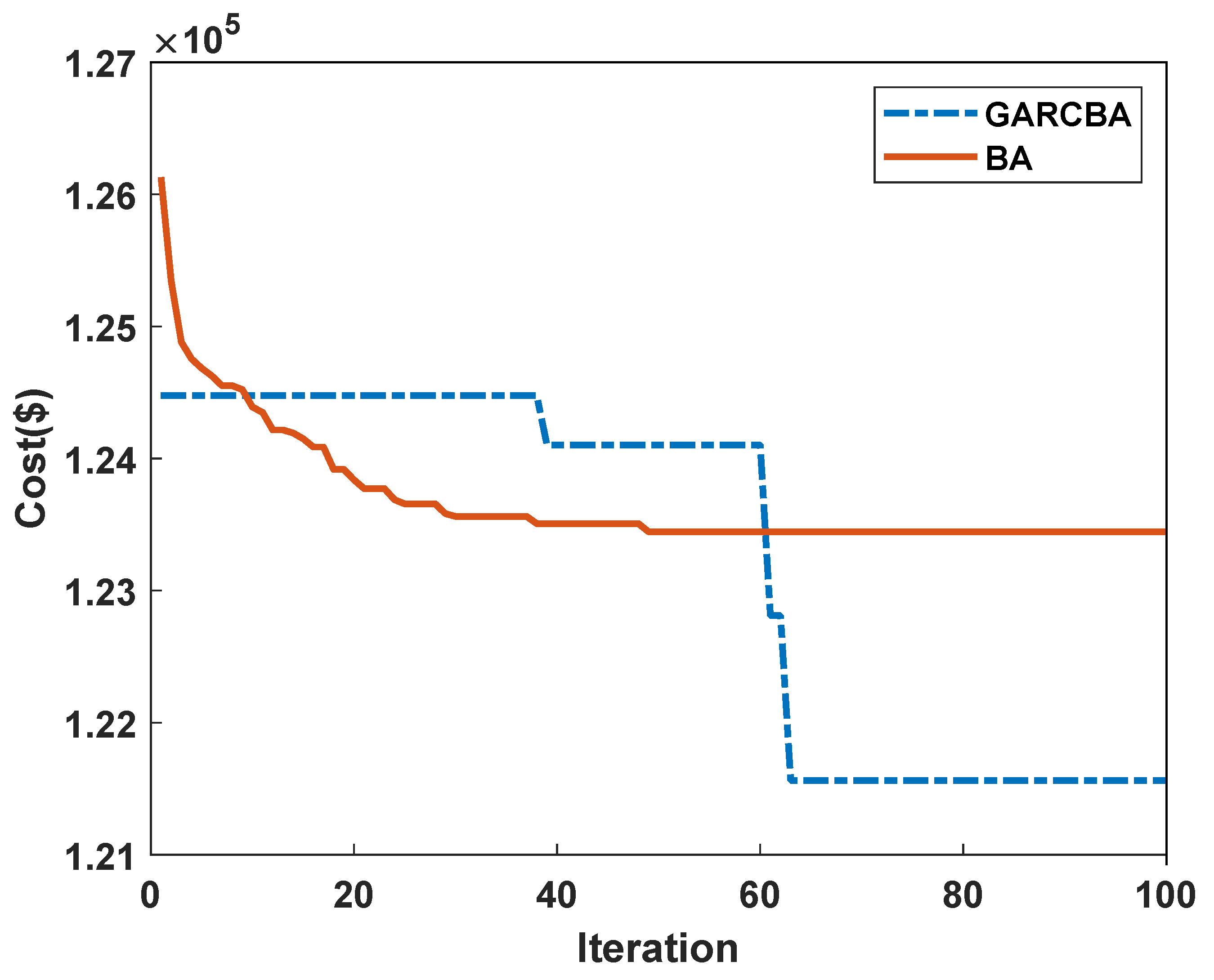
Cost (USD)	121,563.2091	123,757.39	122,936.74

displays the best cost of solving the LED problem using the proposed GARCBA compared with the BA and BA-Penalty [50] in the IEEE 40-unit test system. Table 9 shows the GARCBA produces the better results in terms of minimum total cost compared with other algorithms. The optimal cost is USD 121,563.2091/h.

Table 10. Statistical results for Case 3.1.

Algorithm		Fuel Cost (USD)		Mean Time (s)
	Minimum	Maximum	Average
GARCBA	121,563.2091	122,089.762	122,432.1055	32.5984
BA [50]	123,757.39	128,510.43	125,979.26	NA
BA-Penalty [50]	122,936.74	129,218.58	126,093.09	NA
MBA [51]	121,578.4856	121,601.0042	121,583.3047	NA
ESO [52]	122,122.1600	123,143.0700	122,558.4565	NA

shows a comparison of the GARCBA’s statistical results with other algorithms. The GARCBA optimization process is implemented for 25 trials. Although the GARCBA is slightly less stable than the MBA [51], it is clear that it performs better in terms of minimum total cost of ownership. The GARCBA’s average execution time is 32.5984 s.

5.3.2. Case 3.2: Valve-Point Effect and POZs Are Considered

To make the test system more realistic, we considered the valve-point effect in this case. The parameters of the valve-point effect are shown in Table A3. The GARCBA’s parameters are the same as in Case 3.1.

Table 11. Best cost solutions for Case 3.2.

Items	GARCBA	NGWO [10]	PSO-LRS [53]	Items	GARCBA	NGWO [10]	PSO-LRS [53]
$P_1$	95.3933	111.3177	111.9858	$P_{21}$	522.0699	526.1137	523.4072
$P_2$	91.3479	112.7551	110.5273	$P_{22}$	546.3573	532.1443	523.4599
$P_3$	106.9435	118.6377	98.5560	$P_{23}$	496.7465	536.8421	523.4756
$P_4$	164.2468	183.3649	182.9622	$P_{24}$	501.5560	524.4669	523.7032
$P_5$	84.5461	91.8097	87.7254	$P_{25}$	546.5400	525.2461	523.7854
$P_6$	121.5171	104.3697	139.9933	$P_{26}$	533.9505	529.3289	523.2757
$P_7$	233.2553	297.6533	259.6628	$P_{27}$	121.3725	9.9500	10.0000
$P_8$	297.5397	289.4349	297.7912	$P_{28}$	78.7507	9.9500	10.6251
$P_9$	271.7046	298.4044	284.8459	$P_{29}$	98.2577	9.9500	10.0727
$P_{10}$	266.2047	129.3500	130.0000	$P_{30}$	89.8568	88.4106	51.3321
$P_{11}$	215.7838	241.9702	94.6741	$P_{31}$	183.2669	188.9088	189.8048
$P_{12}$	368.1091	166.9113	94.3734	$P_{32}$	76.9153	188.8126	189.7386
$P_{13}$	250	214.8490	214.7369	$P_{33}$	162.4044	186.9624	189.9122
$P_{14}$	200	215.6690	394.1370	$P_{34}$	159.7818	195.0897	199.3258
$P_{15}$	425.2913	305.6922	483.1816	$P_{35}$	183.9541	171.5047	199.3065
$P_{16}$	214.1350	394.6479	304.5381	$P_{36}$	186.7423	176.1085	192.8977
$P_{17}$	434.3557	494.7618	489.2139	$P_{37}$	101.6365	89.5297	109.8628
$P_{18}$	469.7557	493.1559	489.6154	$P_{38}$	77.0279	89.3589	111.304
$P_{19}$	503.7925	512.7416	511.1782	$P_{39}$	105.4998	109.3222	92.8751
$P_{20}$	523.5192	520.8929	511.7336	$P_{40}$	433.9072	512.5412	511.6883
Cost (USD)	121,768.1229	121,881.81	122,035.7946

shows the detailed best solution of Case 3.2 with the GARCBA, NGWO [10], and PSO-LRS [53]. Table 11 shows the best cost obtained by the proposed GARCBA is 121,768.1229 USD/h. To further explain the superior performance of the GARCBA in solving the LED problem of a 40-unit test system, we show a comparison between the statistical results obtained by the GARCBA and the other algorithms in

Table 12. Statistical results for Case 3.2.

Algorithm		Fuel Cost (USD)		Mean Time (s)
	Minimum	Maximum	Average
GARCBA	121,768.1229	121,801.0585	121,864.9455	28.3488
NGWO [10]	121,881.81	NA	122,787.77	NA
PSO-LRS[53]	122,035.7946	NA	122,558.4565	NA
IGA [54]	121,915.93	NA	122,811.41	NA
PSO [55]	123,930.45	123,143.0700	124,154.49	933.39
CJAYA [53]	121,799.88	NA	122,581.85	NA
CPSO [56]	121,865.23	NA	122,100.87	114.65
DEC-SQP [57]	121,741.9793	122,981.5913	122,295.1278	386.1809

. The GARCBA outperforms other algorithms in terms of minimum, maximum, and average values over 25 runs. Additionally, the best running time is 28.3488 s, which is also obtained from the GARCBA.

6. Conclusions

In this paper, to solve the LED problem in a short time, we proposed and applied a surrogate-assisted adaptive bat algorithm to the IEEE 118- and 300-bus systems, as well as an IEEE 40-unit test system. On the one hand, we used a GRNN to approximate the cost function of LED problems to reduce the computational cost of obtaining fitness values. Furthermore, we integrated a self-adaptive “minimizing the predictor” sampling strategy into the original GRNN to improve the accuracy online. The abundant execution times of LED problems are reduced by using the GRNN surrogate model. On the other hand, to obtain a better, more stable solution for the LED problem, we proposed the GARCBA to execute LED optimization problems. Furthermore, compared with the original RCBA, ESE ensures the reliability of the GARCBA. Moreover, we proposed an average evolutionary factor for the adaptive updating of random black hole radius in the GARCBA. Our simulation experiments demonstrate the superiority of the GARCBA in solving LED problems. In our paper, we studied the static LED problem; however, a future study of dynamic LED involving renewable energy would provide another direction.

References

- Alawode, K.O.; Jubril, A.M.; Kehinde, L.O.; Ogunbona, P.O. Semidefinite programming solution of economic dispatch problem with non-smooth, non-convex cost functions. Electr. Power Syst. Res. 2018, 164, 178–187. [Google Scholar] [CrossRef]
- Shuai, H.; Fang, J.; Ai, X.; Tang, Y.; Wen, J.; He, H. Stochastic Optimization of Economic Dispatch for Microgrid Based on Approximate Dynamic Programming. IEEE Trans. Smart Grid 2019, 10, 2440–2452. [Google Scholar] [CrossRef] [Green Version]
- Zhan, J.P.; Wu, Q.H.; Guo, C.X.; Zhou, X.X. Fast λ-iteration method for economic dispatch with prohibited operating zones. IEEE Trans. Power Syst. 2013, 29, 990–991. [Google Scholar] [CrossRef]
- Guo, Y.; Tong, L.; Wu, W.C.; Zhang, B.M.; Sun, H.B. Coordinated multi-area economic dispatch via critical region projection. IEEE Trans. Power Syst. 2017, 32, 3736–3746. [Google Scholar] [CrossRef]
- Ponciroli, R.; Stauff, N.E.; Ramsey, J.; Ganda, F.; Vilim, R.B. An improved genetic algorithm approach to the unit commitment/economic dispatch problem. IEEE Trans. Power Syst. 2020, 35, 4005–4013. [Google Scholar] [CrossRef]
- Xu, S.; Xiong, G.; Mohamed, A.W.; Bouchekara, H.R. Forgetting velocity based improved comprehensive learning particle swarm optimization for non-convex economic dispatch problems with valve-point effects and multi-fuel options. Energy 2022, 256, 124511. [Google Scholar] [CrossRef]
- Al-Rubayi, R.H.; Abd, M.K.; Flaih, F.M. A new enhancement on PSO algorithm for combined economic-emission load dispatch issues. Int. J. Intell. Eng. Syst. 2020, 13, 77–85. [Google Scholar] [CrossRef]
- Liang, H.J.; Liu, Y.G.; Shen, Y.J.; Li, F.Z.; Man, Y.C. A hybrid bat algorithm for economic dispatch with random wind power. IEEE Trans. Power Syst. 2018, 33, 5052–5061. [Google Scholar] [CrossRef]
- Ellahi, M.; Abbas, G.; Satrya, G.B.; Usman, M.R.; Gu, J. A modified hybrid particle swarm optimization with bat algorithm parameter inspired acceleration coefficients for solving eco-friendly and economic dispatch problems. IEEE Access 2021, 9, 82169–82187. [Google Scholar] [CrossRef]
- Xu, J.; Yan, F.; Yun, K.; Su, L.; Li, F.; Guan, J. Noninferior Solution Grey Wolf Optimizer with an Independent Local Search Mechanism for Solving Economic Load Dispatch Problems. Energies 2019, 12, 2274. [Google Scholar] [CrossRef]
- Pothiya, S.; Ngamroo, I.; Kongprawechnon, W. Ant colony optimisation for economic dispatch problem with non-smooth cost functions. Int. J. Elect. Power Energy Syst. 2010, 32, 478–487. [Google Scholar] [CrossRef]
- Yang, X.S.; Hosseini, S.S.S.; Gandomi, A.H. Firefly algorithm for solving non-convex economic dispatch problems with valve loading effect. Appl. Soft Comput. 2012, 12, 1180–1186. [Google Scholar] [CrossRef]
- Basu, M.; Chowdhury, A. Cuckoo search algorithm for economic dispatch. Energy 2013, 60, 99–108. [Google Scholar] [CrossRef]
- Noman, N.; Iba, H. Differential evolution for economic load dispatch problems. Electr. Power Syst. Res. 2008, 80, 1322–1331. [Google Scholar] [CrossRef]
- Gholamghasemi, M.; Akbari, E.; Asadpoor, M.B.; Ghasemi, M. A new solution to the non-convex economic load dispatch problems using phasor particle swarm optimization. Appl. Soft Comput. 2019, 79, 111–124. [Google Scholar] [CrossRef]
- Dubey, S.M.; Dubey, H.M.; Salkuti, S.R. Modified Quasi-Opposition-Based Grey Wolf Optimization for Mathematical and Electrical Benchmark Problems. Energies 2022, 15, 5704. [Google Scholar] [CrossRef]
- El-Sehiemy, R.; Shaheen, A.; Ginidi, A.; Elhosseini, M. A Honey Badger Optimization for Minimizing the Pollutant Environmental Emissions-Based Economic Dispatch Model Integrating Combined Heat and Power Units. Energies 2022, 15, 7603. [Google Scholar] [CrossRef]
- Alghamdi, A.S. Greedy Sine-Cosine Non-Hierarchical Grey Wolf Optimizer for Solving Non-Convex Economic Load Dispatch Problems. Energies 2022, 15, 3904. [Google Scholar] [CrossRef]
- Said, M.; Houssein, E.H.; Deb, S.; Ghoniem, R.M.; Elsayed, A.G. Economic Load Dispatch Problem Based on Search and Rescue Optimization Algorithm. IEEE Access 2022, 10, 47109–47123. [Google Scholar] [CrossRef]
- Al-Betar, M.A.; Awadallah, M.A.; Abu-Doush, I.; Alsukhni, E.; Alkhraisat, H. A non-convex economic dispatch problem with valve loading effect using a new modified β-Hill climbing local search algorithm. Arab. J. Sci. Eng. 2018, 43, 7439–7456. [Google Scholar] [CrossRef]
- Chiang, C.L. Improved genetic algorithm for power economic dispatch of units with valve-point effects and multiple fuels. IEEE Trans. Power Syst. 2005, 20, 1690–1699. [Google Scholar] [CrossRef]
- Jin, Y. Surrogate-assisted evolutionary computation: Recent advances and future challenges. Swarm Evol. Comput. 2011, 1, 61–70. [Google Scholar] [CrossRef]
- Song, Z.; Wang, H.; He, C.; Jin, Y. A Kriging-Assisted Two-Archive Evolutionary Algorithm for Expensive Many-Objective Optimization. IEEE Trans. Evol. Comput. 2021, 25, 1013–1027. [Google Scholar] [CrossRef]
- Qian, J.; Yi, J.; Cheng, Y.; Liu, J.; Zhou, Q. A sequential constraints updating approach for Kriging surrogate model-assisted engineering optimization design problem. Eng. Comput. 2020, 36, 993–1009. [Google Scholar] [CrossRef]
- Guo, D.; Wang, X.; Gao, K.; Jin, Y.; Ding, J.; Chai, T. Evolutionary Optimization of High-Dimensional Multiobjective and Many-Objective Expensive Problems Assisted by a Dropout Neural Network. IEEE Trans. Syst. Man Cybern. 2022, 52, 2084–2097. [Google Scholar] [CrossRef]
- Sun, G.; Wang, S. A review of the artificial neural network surrogate modeling in aerodynamic design. P I Mech. Eng. G-J. AER 2019, 233, 5863–5872. [Google Scholar] [CrossRef]
- Kurtulus, E.; Yildiz, A.R.; Sait, S.M.; Bureerat, S. A novel hybrid Harris hawks-simulated annealing algorithm and RBF-based metamodel for design optimization of highway guardrails. Mater. Test. 2020, 62, 251–260. [Google Scholar] [CrossRef]
- Yan, C.; Yin, Z.; Shen, X.; Mi, D.; Guo, F.; Long, D. Surrogate-based optimization with improved support vector regression for non-circular vent hole on aero-engine turbine disk. Aerosp. Sci. Technol. 2020, 96, 105332. [Google Scholar] [CrossRef]
- Wang, H.; Jin, Y.; Sun, C.; Doherty, J. Offline data-driven evolutionary optimization using selective surrogate ensembles. IEEE Trans. Evol. Comput. 2018, 23, 203–216. [Google Scholar] [CrossRef]
- Park, J.; Kim, K.Y. Meta-modeling using generalized regression neural network and particle swarm optimization. Appl. Soft Comput. 2017, 51, 354–369. [Google Scholar] [CrossRef]
- Wang, Y.; Yin, D.Q.; Yang, S.; Sun, G. Global and local surrogate-assisted differential evolution for expensive constrained optimization problems with inequality constraints. IEEE Trans. Cybern. 2018, 39, 1642–1656. [Google Scholar] [CrossRef] [PubMed] [Green Version]
- Gheyas, I.A.; Smith, L.S. Feature subset selection in large dimensionality domains. Pattern Recognit 2010, 43, 1–13. [Google Scholar] [CrossRef] [Green Version]
- Alexandrov, N.M.; Dennis, J.E.; Lewis, R.M.; Torczon, V. A trust-region framework for managing the use of approximation models in optimization. Struct. Optim. 1998, 15, 16–23. [Google Scholar] [CrossRef]
- Dong, H.; Song, B.; Wang, P.; Huang, S. A kind of balance between exploitation and exploration on kriging for global optimization of expensive functions. J. Mech. Sci. Technol. 2015, 29, 2121–2133. [Google Scholar] [CrossRef]
- Aalimahmoody, N.; Bedon, C.; Hasanzadeh-Inanlou, N.; Hasanzade-Inallu, A.; Nikoo, M. Bat algorithm-based ANN to predict the compressive strength of concrete—A comparative study. Infrastructures 2021, 6, 80. [Google Scholar] [CrossRef]
- Guerraiche, K.; Dekhici, L.; Chatelet, E.; Zeblah, A. Multi-objective electrical power system design optimization using a modified bat algorithm. Energies 2021, 14, 3956. [Google Scholar] [CrossRef]
- Said, M.; El-Rifaie, A.M.; Tolba, M.A.; Houssein, E.H.; Deb, S. An efficient chameleon swarm algorithm for economic load dispatch problem. Mathematics 2021, 9, 2770. [Google Scholar] [CrossRef]
- Qi, Y.; Cai, Y. Hybrid chaotic discrete bat algorithm with variable neighborhood search for vehicle routing problem in complex supply chain. Appl. Sci. 2021, 11, 10101. [Google Scholar] [CrossRef]
- Tariq, F.; Alelyani, S.; Abbas, G.; Qahmash, A.; Hussain, M.R. Solving Renewables-Integrated Economic Load Dispatch Problem by Variant of Metaheuristic Bat-Inspired Algorithm. Energies 2020, 13, 6225. [Google Scholar] [CrossRef]
- Rugema, F.X.; Yan, G.; Mugemanyi, S.; Jia, Q.; Zhang, S.; Bananeza, C. A cauchy-Gaussian quantum-behaved bat algorithm applied to solve the economic load dispatch problem. IEEE Access 2020, 9, 3207–3228. [Google Scholar] [CrossRef]
- Liang, H.; Liu, Y.; Li, F.; Shen, Y. A multiobjective hybrid bat algorithm for combined economic/emission dispatch. Int. J. Elect. Power Energy Syst. 2018, 101, 103–115. [Google Scholar] [CrossRef]
- Zhan, Z.H.; Zhang, J.; Li, Y.; Chung, H.S.H. Adaptive particle swarm optimization. IEEE Trans. Syst. Man Cybern. Syst. 2009, 39, 1362–1381. [Google Scholar] [CrossRef] [PubMed] [Green Version]
- Pan, S.; Jian, J.; Yang, L. A hybrid MILP and IPM approach for dynamic economic dispatch with valve-point effects. Int. J. Elect. Power Energy Syst. 2018, 97, 290–298. [Google Scholar] [CrossRef] [Green Version]
- Chaib, A.E.; Bouchekara, H.R.E.H.; Mehasni, R.; Abido, M.A. Optimal power flow with emission and non-smooth cost functions using backtracking search optimization algorithm. Int. J. Elect. Power Energy Syst. 2016, 81, 64–77. [Google Scholar] [CrossRef]
- Specht, D.F. General regression neural network. IEEE Trans. Neural Netw. 1991, 2, 568–576. [Google Scholar] [CrossRef] [Green Version]
- Parzen, E. On estimation of a probability density function and mode. Ann. Math. Stat. 1962, 33, 1065–1076. Available online: http://www.jstor.org/stable/2237880 (accessed on 9 December 2022). [CrossRef]
- Tian, Y.; Cheng, R.; Zhang, X.; Jin, Y. A MATLAB platform for evolutionary multi-objective optimization [educational forum]. IEEE Comput. Intell. Mag. 2017, 12, 73–87. [Google Scholar] [CrossRef] [Green Version]
- Muthuswamy, R.; Krishnan, M.; Subramanian, K.; Subramanian, B. Environmental and economic power dispatch of thermal generators using modified NSGA-II algorithm. Int. Trans. Electr. Energy Syst. 2015, 25, 1552–1569. [Google Scholar] [CrossRef]
- Zimmerman, R.; Gan, D. MATPOWER—A MATLAB Power System Simulation Package. 2009. Available online: http://www.pserc.cornell.edu/matpower (accessed on 26 December 2022).
- Karakonstantis, I.; Vlachos, A. Bat algorithm applied to continuous constrained optimization problems. Inf. Sci. 2021, 42, 57–75. [Google Scholar] [CrossRef]
- Baziar, A.; Rostami, M.A.; Akbari-Zadeh, M.R. An intelligent approach based on bat algorithm for solving economic dispatch with practical constraints. Int. J. Fuzzy Syst. 2014, 27, 1601–1607. [Google Scholar] [CrossRef]
- Pereira-Neto, A.; Unsihuay, C.; Saavedra, O.R. Efficient evolutionary strategy optimization procedure to solve the nonconvex economic dispatch problem with generator constraints. Proc. Inst. Elect. Eng. Gen. Transm. Distrib. 2005, 152, 653–660. [Google Scholar] [CrossRef]
- Wang, Y.-K.; Chen, X.-B. Improved multi-area search and asymptotic convergence PSO algorithm with independent local search mechanism. Control Decis. 2018, 33, 1382–1389. [Google Scholar]
- Ling, S.H.; Leung, F.H.F. An Improved genetic algorithm with average-bound crossover and wavelet mutation operation. Soft Comput. 2007, 11, 7–31. [Google Scholar] [CrossRef] [Green Version]
- Kumar, R.; Sharma, D.; Sadu, A. A hybrid multi-agent based particle swarm optimization algorithm for economic power dispatch. Int. J. Electr. Power Energy Syst. 2011, 33, 115–123. [Google Scholar] [CrossRef]
- Victoire, T.A.A.; Jeyakumar, A.E. Hybrid PSO–SQP for economic dispatch with valve-point effect. Elect. Power Syst. Res. 2004, 71, 51–59. [Google Scholar] [CrossRef]
- Coelho, L.D.S.; Mariani, V.C. Combining of chaotic differential evolution and quadratic programming for economic dispatch optimization with valve-point effect. IEEE Trans. Power Syst. 2006, 21, 989–996. [Google Scholar] [CrossRef]