Coordinated Dispatch Optimization between the Main Grid and Virtual Power Plants Based on Multi-Parametric Quadratic Programming

Abstract

Virtual power plants (VPPs) are a critical technology for distribution systems that can integrate various renewable energy resourcescontrollable loads and energy storage systems into one specific power plant through a distributed energy management system. This paper proposes a coordinated dispatch optimization model between the main grid and VPPs aiming to minimize both the power generation cost and total system active loss. When the time of the equivalent dispatching model is not divisible due to the existence of a time coupling constraint inside the VPPs, this model can obtain the global optimal solution through iteration between the main grid and the VPPs. By employing multi-parametric quadratic programming to obtain accurate critical domains and optimal cost functions, the convergence speed and stability are significantly improved. Additionally, a reactive power and voltage optimization technique leveraging the generalized Benders decomposition is presented for the coordination of the main grid and the VPPs. Moreover, the impact of distributed energy resource (DER) clusters on the main grid was studied, from which we proved that the proposed approach can expeditiously abate energy production expenditure and system active dissipation whilst enhancing the system equilibrium.

1. Introduction

Distributed energy resources (DERs) have many advantages such as low pollution, high energy utilization efficiency, and low investment and construction costs [1,2,3]. The rapid expansion of distributed generators has caused DER technologies to become prevalent, which play an important part in energy markets [4]. However, there are many problems in their actual operation and application processes, such as the high cost of a single distributed power supply and coordination and control difficulties. To address these problems, the concept of virtual power plants (VPPs) has been introduced into grid control [5], which can coordinate and control DERs effectively, thus enabling their seamless integration into the main grid. They can exist as cloud power plants, which aggregate heterogeneous DERs to form a single operating unit to facilitate the management of individual DERs, enabling system operators to develop dispatch optimization strategies [6].

Moreover, the decarbonization of the energy system has driven many studies about DER aggregators with network operators. António Coelho et al. [7] proposed a market participation of aggregators of multi-energy systems. The alternating direction method of multipliers (ADMM) was utilized in their paper, in which the aggregator worked together with the operators of electricity, gas and heat networks to calculate network-secure bids to ensure the network’s reliability and stability. Jose Iria et al. [8] presented a new bidding optimization strategy for an aggregator of prosumers to make decisions in real-time markets. The bidding strategy employed the ADMM within a rolling horizon framework to facilitate the negotiation of MV-LV network-secure bids between the aggregator and DSO while maintaining the data privacy of both parties. Nuno Soares Fonseca et al. [9] presented a novel decentralized framework for distribution system operators (DSOs) to assess the network feasibility of aggregator bids and compensate them for providing network support services. These studies have played a crucial role in facilitating the integration of DERs into the grid.

However, with the increasing penetration of DERs, VPPs using centralized energy management and dispatching operations face many problems such as high communication costs, low optimization efficiency, and variable operating conditions of distributed power sources, and it is difficult to coordinate the randomness and volatility of a large number of uncontrollable power sources [10,11]. This forces the main grid to act as a power backup for DERs and VPPs, which impacts the main grid, thereby increasing the difficulty of its operational control. In order to improve the observability and controllability of VPPs and make the most of the coordination capabilities of VPPs to control DERs, it is urgent to study the coordinated and optimal control technology of DER clusters to realize the full consumption and optimal control of DERs in distribution systems [12,13,14].

There are some methodologies about optimal scheduling for VPPs. Wang et al. [15] proposed an economic operation optimization model based on a modified genetic algorithm with the voltage control requirements of VPP scheduling considered. Vale et al. [16] presented a multi-level consultation mechanism that leverages the advantages of VPP management to achieve optimal operation and negotiation in power markets with smart grids. Bertram et al. [17] used a reactive power supply control model to analyze the small-signal stability of voltage regulation in medium-voltage distribution networks. Ruthe et al. [18] introduced a new distributed coordination algorithm as well as the concept of direct control to allow small loads or generator sets to provide a secondary control reserve. Bao et al. [19] analyzed the functions of different resources to ensure the maximum security of a distribution network. Vasirani et al. [20] described electric vehicles as a storage medium connected to wind turbines. They suggested an agent-oriented methodology to refine its grid-energy-provisioning strategies and leverage energy storage to maximize profits in response to uncertainties associated with wind power forecasts. Zhu et al. [21] considered the uncertainty of DERs and load and proposed a mapping method and a two-layer optimization method to solve the dynamic dispatch problem of VPPs. Giuntoli et al. [22] proposed a novel model to solve the day-ahead thermoelectric and electrical optimization of VPPs problem, which also considered the precise geospatial coordinates of each DER within the main grid and its unique characteristics. They demonstrated how the promise of clusters of DERs at virtual public coupling points affects optimal VPP operations in microgrids and active distribution networks.

However, there has been a lack of research on coordinated scheduling between VPPs and the main grid. The transition from centralized to distributed energy resources brings the diversity of variables in smart grids [23]. The intermittent generation of heterogeneous DERs can destabilize the system and result in significant fluctuations. Time-varying market prices and flexible load demands cause uncontrollable confusion in the deployment system [24,25,26]. These tasks necessitate the development of a flexible operation control strategy to consider the optimal dispatching process of VPPs and the main grid, to alleviate conflicts and to facilitate energy trading.

In this paper, we comprehensively study the dynamic scheduling method of the coordination between the main grid and VPPs, considering the cost of energy production and system active loss. A multi-parameter planning projection algorithm for the hierarchical coordination control of VPPs and the power grid is proposed, which improves the convergence by more than one order of magnitude, realizes the combination of centralized online coordination optimization and local fast control of the power supply and solves the difficult problem of the centralized control of a large-scale distributed power supply. The operational framework is shown in Figure 1. The contribution of our work contains the following features:

First, a dynamic economic scheduling model for the coordination of the main grid and VPPs is presented. We adopted an iterative strategy to address the time inseparability of the equivalent scheduling model caused by time coupling constraints. Our method can obtain the global optimal solution even when there are time coupling constraints inside the VPPs. We employed multi-parametric quadratic programming to generate the precise critical domain and the optimal cost function, which significantly improved the convergence speed and stability.

Then, for reactive power and voltage optimization between the main grid and VPPs, we leveraged the generalized Benders decomposition with an expeditious practicable cut generation algorithm to reduce the system active loss. We utilized the second-order cone programming relaxation method for reactive VPP optimization as an ancillary task. After relaxation, the subproblem becomes convex, ensuring convergence. Moreover, the proposed method can prevent the overvoltage caused by massive access to DERs in VPPs.

Finally, we analyzed the impact of DER cluster operations on the power grid. If there is no coordination between the main grid and VPPs, power flow reversal and voltage limit violations may occur when a large number of DERs are injected into the power grid. To address this issue, we presented a robust optimal power flow model that considers the uncertainty of the DER and provides strategies with better comprehensive economic benefits for different scenarios.

This paper is structured as follows: Section 2 elucidates the main grid–VPPs decomposition coordinated dispatch model, which considers the power generation cost and system loss. Section 3 provides the problem analysis and solutions. In Section 4, we show our case study. In Section 5, we present an assessment of the implications of the DER cluster operation on the smart grid. Finally, Section 6 offers a summation of our approach.

2. Materials and Methods

In this section, we present our economic optimization and reactive power and voltage control model for the coordination between the main grid and VPPs. The coordination between the main grid and VPPs is showcased in Figure 2. The circled part is the VPP, and the DERs are seen as a resource cluster of it. The red line density is the main grid. This paper mainly focuses on the coordination and interaction between the main grid and VPPs.

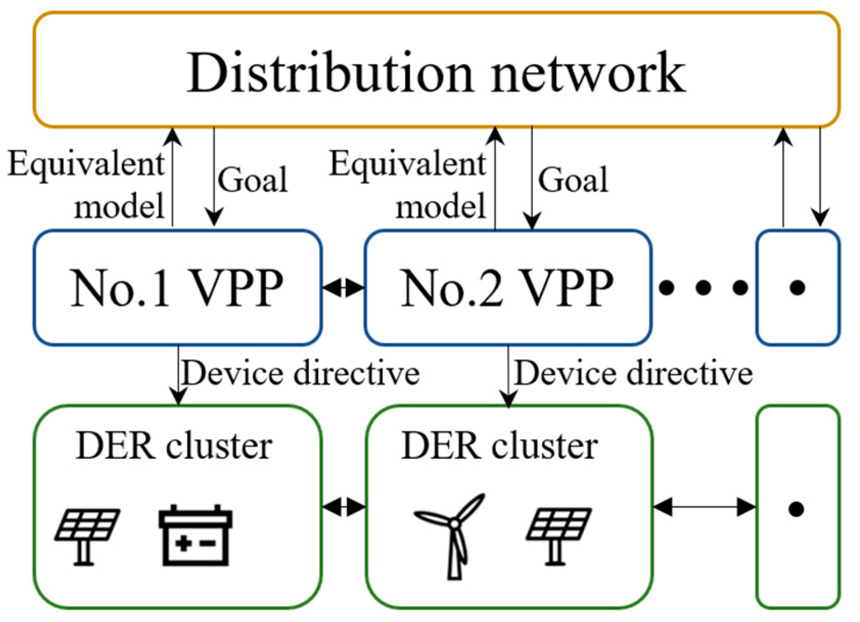
2.1. Coordinated Dispatch Model between Main Grid and VPPs

To achieve dynamic scheduling coordination, our goal was to minimize the aggregate generation costs and losses. The former focuses on the economic dispatch between the VPPs and the main grid in order to minimize power generation costs. The latter considers reactive voltage control to minimize the total network losses. The equations are illustrated by the following formulas:

$$\min \left(Cost+Loss\right)$$

(1a)

$$Cost={\displaystyle \sum _{t\in T}{\displaystyle \sum _{i\in G^{trans}}{C}_i^{trans}\left(p{g}_{i,t}^{trans}\right)}}+{\displaystyle \sum _{t\in T}{\displaystyle \sum _{k\in DIST}{\displaystyle \sum _{i\in G^{dist,k}}{C}_i^{dist,k}\left(p{g}_{i,t}^{dist,k}\right)}}}$$

(1b)

$$Loss={\displaystyle \sum _{i\in I^{trans}}\left(P_{Gi}^{trans}-P_{Di}^{trans}\right)}+{\displaystyle \sum _{k\in DIST}{\displaystyle \sum _{i\in I^{dist,k}}\left(P_{Gi}^{dist,k}-P_{Di}^{dist,k}\right)}}$$

(1c)

The cost function is as follows:

$$C_i\left(p{g}_{i,t}\right)=a_{0,i}+a_{1,i}p{g}_{i,t}+a_{2,i}p{g}_{i,t}^2$$

(2)

where $T$ is the set of dispatching moments, $G$ is the set of nodes where generator sets are located, $I$ is the set of a node index, and $DIST$ is the set of VPPs. The superscript ${\left(·\right)}^{trans}$ denotes the variable/function/set of the main network, while superscript ${\left(·\right)}^{dist,k}$ denotes the variable/function/set of the $k\mathrm{th}$ VPP. The function $C_i\left(·\right)$ represents the power generation cost function of the generator set of node $i$, and $p{g}_{i,t}$ represents the output of the generator set of node $i$ at time $t$. $P_{Gi}^{}$ and $P_{Di}^{}$ are the active injection and load of the generator $i$. $a_{0,i}$, $a_{1,i}$ and $a_{2,i}$ are the power generation cost constant, primary term and secondary term, respectively, of the generator set at node $i$.

2.1.1. Main Grid Model

In the main grid, the generation set needs to satisfy the following constraints:

Power balance constraints:

$${\displaystyle \sum _{i\in G^{trans}}p{g}_{i,t}^{trans}}={\displaystyle \sum _{i\in B^{trans}}p{b}_{i,t}^{trans}}+{\displaystyle \sum _{i\in D^{trans}}P{D}_{i,t}^{trans}},\forall t\in T$$

(3)

where $B$ is the set of boundary nodes between the main network and the VPP, and $D$ is the set of load nodes. The variable $p{b}_{i,t}^{trans}$ represents the power transmitted from node $i$ to the VPP at time $t$, and $P{D}_{i,t}$ represents the load forecast value of node $i$ at time $t$.

Power flow constraints:

$$P_{ij}^{trans}={\left(V_i^{trans}\right)}^2{G}_{ij}^{trans}-V_i^{trans}{V}_j^{trans}\left(G_{ij}^{trans}\cos {\theta }_{ij}^{trans}+B_{ij}^{trans}\sin {\theta }_{ij}^{trans}\right)$$

(4)

$$Q_{ij}^{trans}={\left(V_i^{trans}\right)}^2{B}_{ij}^{trans}-V_i^{trans}{V}_j^{trans}\left(G_{ij}^{trans}\sin {\theta }_{ij}^{trans}-B_{ij}^{trans}\cos {\theta }_{ij}^{trans}\right)$$

(5)

$${\displaystyle \sum _{j\in \pi (i)}{P}_{ij}^{trans}}=P_{Gi}^{trans}-P_{Di}^{trans}$$

(6)

$${\displaystyle \sum _{j\in \pi (i)}{Q}_{ij}^{trans}}=Q_{Gi}^{trans}-Q_{Di}^{trans}$$

(7)

Constraints (4) and (5) ($P_{ij}$ and $Q_{ij}$) are the active and reactive power flow formulas of branch $ij$, where $G_{ij}$ and $B_{ij}^{}$ are the conductance and susceptance of the branch connecting nodes $i$ and $j$, respectively. $V_i^{}$ and $V_j^{}$ represent the voltage amplitude of nodes $i$ and $j$, and ${\theta }_{ij}$ represents the phase angle of branch $ij$. Constraints (6) and (7) are for the active and reactive power balances, where $Q_{Gi}^{}$ and $Q_{Di}^{}$ represent the reactive injection and load of node $i$, and $\pi (i)$ represents the set of nodes directly connected to node $i$.

Line transmission capacity constraints:

$$\begin{array}{l}-P{L}_j^{trans}\le {\displaystyle \sum _{i\in G^{trans}}S{F}_{j-i}^{trans}p{g}_{i,t}^{trans}}-{\displaystyle \sum _{i\in B^{trans}}S{F}_{j-i}^{trans}p{b}_{i,t}^{trans}}\\ \hspace{1em}-{\displaystyle \sum _{i\in D^{trans}}S{F}_{j-i}^{trans}P{D}_{i,t}^{trans}}\le P{L}_j^{trans},\forall j\in L^{trans},\forall t\in T\end{array}$$

(8)

where $P{L}_j$ is the transmission capacity of branch $j$, $S{F}_{j-i}$ is the transfer distribution factor from node $i$ to branch $j$, and $L$ is the line set.

Spinning reserve constraint:

$$0\le r{u}_{i,t}^{trans}\le R{U}_i^{trans}\Delta t,r{u}_{i,t}^{trans}\le {\overline{PG}}_i^{trans}-p{g}_{i,t}^{trans},\forall i\in G^{trans},\forall t\in T$$

(9)

$$0\le r{d}_{i,t}^{trans}\le R{D}_i^{trans}\Delta t,r{d}_{i,t}^{trans}\le p{g}_{i,t}^{trans}-{\underset{¯}{PG}}_i^{trans},\forall i\in G^{trans},\forall t\in T$$

(10)

$${\displaystyle \sum _{i\in G^{trans}}r{u}_{i,t}^{trans}}\ge SR{U}_t^{trans},{\displaystyle \sum _{i\in G^{trans}}r{d}_{i,t}^{trans}}\ge SR{D}_t^{trans},\forall t\in T$$

(11)

where $r{u}_{i,t}$ and $r{d}_{i,t}$ represent the upward and downward rotation of the spare capacity of node $i$ at time $t$, respectively. $R{U}_i$ and $R{D}_i$ are the upward and downward ramp rates of node $i$, respectively. $\Delta t$ is the scheduling interval. ${\overline{PG}}_i$ and ${\underset{¯}{PG}}_i$ are the upper and lower limits of the generator set output of node $i$. $SR{U}_t$ and $SR{D}_t$ represent the upward and downward rotation reserve capacity requirements of the system at time $t$, respectively.

Unit ramping constraint:

$$-R{D}_i^{trans}\Delta t\le p{g}_{i,t+1}^{trans}-p{g}_{i.t}^{trans}\le R{U}_i^{trans}\Delta t,\forall i\in G^{trans},\forall t\in T$$

(12)

Unit output constraints:

$${\underset{¯}{PG}}_i^{trans}\le p{g}_{i,t}^{trans}\le {\overline{PG}}_i^{trans},\forall i\in G^{trans},\forall t\in T$$

(13)

Security constraints:

$$P_{Gi,\min }^{trans}\le P_{Gi}^{trans}\le P_{Gi,\max }^{trans}$$

(14)

$$Q_{Gi,\min }^{trans}\le Q_{Gi}^{trans}\le Q_{Gi,\max }^{trans}$$

(15)

$$V_{i,\min }^{trans}\le V_i^{trans}\le V_{i,\max }^{trans}$$

(16)

$${\left(P_{ij}^{trans}\right)}^2+{\left(Q_{ij}^{trans}\right)}^2\le {\left(S_{ij,\max }^{trans}\right)}^2$$

(17)

Constraints (14) and (15) are the active power and reactive power output constraints, where $P_{Gi,\min }$ and $P_{Gi,\max }$ are the minimum and maximum magnitudes of the generator active output of node $i$, and $Q_{Gi,\min }$ and $Q_{Gi,\max }$ are the minimum and maximum magnitudes of the generator reactive output of node $i$. Constraint formula (16) specifies the main grid voltage amplitude limit, where $V_{i,\min }$ and $V_{i,\max }$ are the minimum and maximum voltage magnitudes of node $i$. Constraint formula (17) identifies the transmission capacity constraint for each line, where $S_{ij,\max }$ is the maximum transmission capacity of branch $ij$.

2.1.2. VPP Model

The modeling of the VPPs is similar to that of the main grid.

Power balance constraints:

$$p{b}_t^{dist,k}+{\displaystyle \sum _{i\in G^{dist,k}}p{g}_{i,t}^{dist,k}}={\displaystyle \sum _{i\in D^{dist,k}}P{D}_{i,t}^{dist,k}},\forall t\in T$$

(18)

Line transmission capacity constraints:

$$\begin{array}{l}-P{L}_j^{dist,k}\le {\displaystyle \sum _{i\in G^{dist,k}}S{F}_{j-i}^{dist,k}p{g}_{i,t}^{dist,k}}+{\displaystyle \sum _{i\in B^{dist,k}}S{F}_{j-i}^{dist,k}p{b}_{i,t}^{dist,k}}\\ \hspace{1em}-{\displaystyle \sum _{i\in D^{dist,k}}S{F}_{j-i}^{dist,k}P{D}_{i,t}^{dist,k}}\le P{L}_j^{dist,k},\forall j\in L^{dist,k},\forall t\in T\end{array}$$

(19)

Spinning reserve constraint:

$$0\le r{u}_{i,t}^{dist,k}\le R{U}_i^{dist,k}\Delta t,r{u}_{i,t}^{dist,k}\le {\overline{PG}}_i^{dist,k}-p{g}_{i,t}^{dist,k},\forall i\in G^{dist,k},\forall t\in T$$

(20)

$$0\le r{d}_{i,t}^{dist,k}\le R{D}_i^{dist,k}\Delta t,r{d}_{i,t}^{dist,k}\le p{g}_{i,t}^{dist,k}-{\underset{¯}{PG}}_i^{dist,k},\forall i\in G^{dist,k},\forall t\in T$$

(21)

$${\displaystyle \sum _{i\in G^{dist,k}}r{u}_{i,t}^{dist,k}}\ge SR{U}_t^{dist,k},{\displaystyle \sum _{i\in G^{dist,k}}r{d}_{i,t}^{dist,k}}\ge SR{D}_t^{dist,k},\forall t\in T$$

(22)

Unit ramping constraint:

$$-R{D}_i^{dist,k}\Delta t\le p{g}_{i,t+1}^{dist,k}-p{g}_{i.t}^{dist,k}\le R{U}_i^{dist,k}\Delta t,\forall i\in G^{dist,k},\forall t\in T$$

(23)

Unit output constraints:

$${\underset{¯}{PG}}_i^{dist,k}\le p{g}_{i,t}^{dist,k}\le {\overline{PG}}_i^{dist,k},\forall i\in G^{dist,k},\forall t\in T$$

(24)

Power flow constraints:

Let $L_{ij}^{dist}={\left(I_{ij}^{dist}\right)}^2$ and $U_i^{dist}={\left(V_i^{dist}\right)}^2$, which represent the squared amplitudes of the current and voltage, respectively. The power flow constraints of a VPP are as follows:

$${\left(P_{ij}^{dist}\right)}^2+{\left(Q_{ij}^{dist}\right)}^2\le L_{ij}^{dist}{U}_i^{dist}$$

(25)

$${\displaystyle \sum _{i\in u(j)}\left(P_{ij}^{dist}-L_{ij}^{dist}{r}_{ij}^{dist}\right)}+P_{Gj}^{dist}={\displaystyle \sum _{k\in v(j)}\left(P_{jk}^{dist}\right)}+P_{Dj}^{dist}$$

(26)

$${\displaystyle \sum _{i\in u(j)}\left(Q_{ij}^{dist}-L_{ij}^{dist}{x}_{ij}^{dist}\right)}+Q_{Gj}^{dist}={\displaystyle \sum _{k\in v(j)}\left(Q_{jk}^{dist}\right)}+Q_{Dj}^{dist}$$

(27)

$$U_j^{dist}=U_i^{dist}-2\left(r_{ij}^{dist}{P}_{ij}^{dist}+x_{ij}^{dist}{Q}_{ij}^{dist}\right)+\left({\left(r_{ij}^{dist}\right)}^2+{\left(x_{ij}^{dist}\right)}^2\right)L_{ij}^{dist}$$

(28)

where $r_{ij}$ and $x_{ij}$ are the resistance and impedance of branch $ij$, and $u(i)$ and $v(i)$ are the ancestor and subordinate nodes of node $i$.

Security constraints:

$$P_{Gi,\min }^{dist}\le P_{Gi}^{dist}\le P_{Gi,\max }^{dist}$$

(29)

$$Q_{Gi,\min }^{dist}\le Q_{Gi}^{dist}\le Q_{Gi,\max }^{dist}$$

(30)

$${\left(V_{i,\min }^{dist}\right)}^2\le U_i^{dist}\le {\left(V_{i,\max }^{dist}\right)}^2$$

(31)

$$I_{ij}^{dist}\le I_{ij,\max }^{dist}$$

(32)

Constraints (29) and (30) are the active power and reactive output constraints of the generator $i$. Constraint formula (31) specifies the voltage amplitude limit. Constraint (32) is the transmission capacity constraint for each line, where $I_{ij,\max }$ is the maximum current amplitude of branch $ij$.

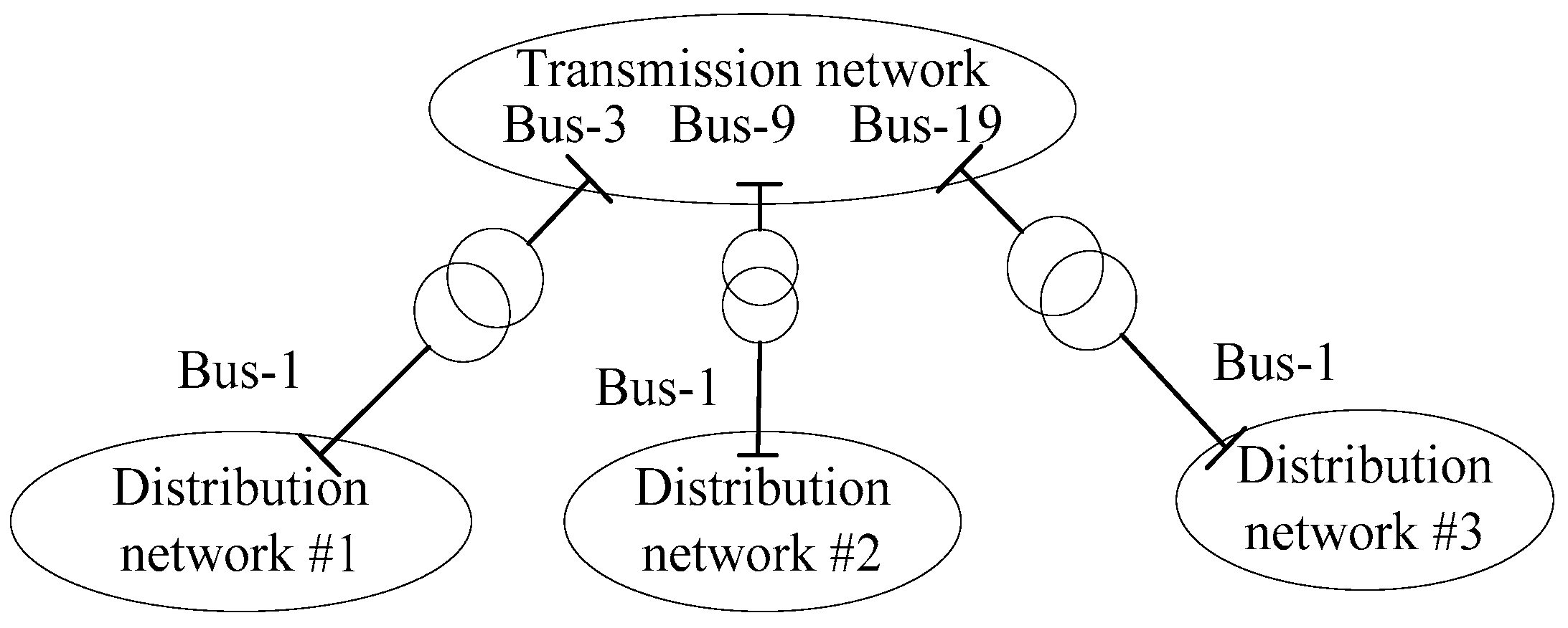
2.1.3. Boundary Conditions

The electricity transmission capacity between the main grid and the VPPs should be balanced as follows:

$$p{b}_{I\left(k\right),t}^{trans}=p{b}_t^{dist,k}$$

(33)

where $I(k)$ is the set of main network nodes that are connected to the $k\mathrm{th}$ VPP.

The DisFlow model must account for certain boundary conditions as follows:

$$V_{T\left(k\right)}^{trans}=V_{root}^{dist,k}$$

(34)

$$P_{T\left(k\right)}^{trans}=P_{root}^{dist,k}$$

(35)

$$Q_{T\left(k\right)}^{trans}=Q_{root}^{dist,k}$$

(36)

where $V_{T\left(k\right)}^{trans}$, $P_{T\left(k\right)}^{trans}$ and $Q_{T\left(k\right)}^{trans}$ are the voltage amplitude, equivalent active power and equivalent reactive power of nodes in the main grid that connect to the $k\mathrm{th}$ VPP, which are equal to $V_{root}^{d,k}$, $P_{root}^{dist,k}$ and $Q_{root}^{dist,k}$, which are the voltage amplitude, active power injection and reactive power injection of the root node in the $k\mathrm{th}$ VPP, respectively.

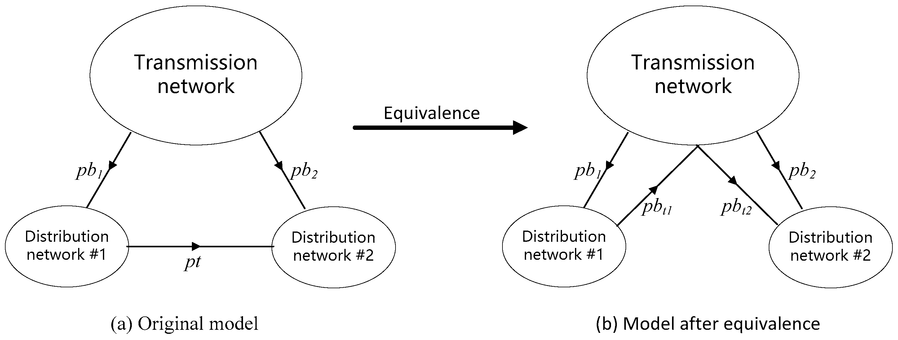
2.1.4. Equivalence of Tie Lines in VPPs

There may be additional connection lines among VPPs, as shown in Figure 2.

The arrow in Figure 3 is the directionality of the active power flow. Recording $pt$ as the power transmitted between VPP 1 and VPP 2, the precedent model (a) can be corresponded to model (b), wherein the main grid receives power, $p{b}_{t1}$, from VPP1 and transmits power, $p{b}_{t2}$, to VPP2 [27]. Then, we have:

$$p{b}_{t1}=p{b}_{t2}=pt$$

(37)

2.2. Robust Optimal Power Flow Considering Impact of DERs on System Operation

The access of many DER clusters requires effective coordination within VPPs. Considering the uncertainty of DERs, a robust optimal power flow model is established.

The robust optimal power flow model reduces the aggregate expenditure in the worst scenario while the requirements are still fulfilled. The uncertainty of DERs is described by the upper and lower limits, which can be addressed as follows:

$$\begin{array}{l}\underset{p_i^G}{\min }\left\{\underset{\Delta P_i^R\in \left[\Delta P_i^{R\min },\Delta P_i^{R\max }\right]}{\max }{\displaystyle \sum _{i\in I^G}\left[C_i^G\left(p_i^G+\Delta p_i^G\right)\right]}\right\}\\ s.t.{\displaystyle \sum _{i\in I^G}{p}_i^G}+{\displaystyle \sum _{i\in I^R}{P}_i^R}={\displaystyle \sum _{i\in I^D}{P}_i^D}+p^{loss}\\ \hspace{1em}\hspace{0.17em}\hspace{0.17em}\hspace{0.17em}{p}^{loss}={\displaystyle \sum _{i\in I^G}{L}_i^G{p}_i^G}+{\displaystyle \sum _{i\in I^R}{L}_i^R{P}_i^R}+P^{LB}\\ \hspace{1em}\hspace{0.17em}\hspace{0.17em}\hspace{0.17em}\Delta p_i^G=-\frac{K_i^G}{1-L_i^G}{\displaystyle \sum _{j\in I^R}\left(1-L_j^R\right)\Delta P_j^R},\forall i\in I^G\\ \hspace{1em}\hspace{0.17em}\hspace{0.17em}\hspace{0.17em}\left|{\displaystyle \sum _{i\in I^G}{S}_{j-i}^G\left(p_i^G+\Delta p_i^G\right)}+{\displaystyle \sum _{i\in I^R}{S}_{j-i}^R\left(P_i^R+\Delta P_i^R\right)}-{\displaystyle \sum _{i\in I^D}{S}_{j-i}^D{P}_i^D}\right|\\ \hspace{1em}\hspace{1em}\hspace{1em}\le P_j^L,\forall j\in I^L\\ \hspace{1em}\hspace{0.17em}\hspace{0.17em}\hspace{0.17em}{P}_i^{G\min }\le p_i^G+\Delta p_i^G\le P_i^{G\max },\forall i\in I^G\end{array}$$

(38)

where $p_i^G$ and $C_i^G\left(p_i^G\right)$ are the power generation output and cost function of conventional generator set $i$, $P_i^R$ is the power generation output of RE unit $i$, $P_i^D$ is the power demand of load $i$, $p^{loss}$ is the total network loss of the system, $L_i^G$ and $L_i^R$ are the linear coefficients of conventional generator $i$ and RE unit $i$, $P^{LB}$ is a constant term and $K_i^G$ is the adjustment factor for each conventional generator set. $I^G$, $I^R$, $I^D$ and $I^L$ are the set of conventional generator sets, RE units, loads and lines in the system. $P_i^{G\min }$ and $P_i^{G\max }$ are the lower and upper bounds of the power generation output of conventional generator set $i$, respectively. $S_{j-i}^G$, $S_{j-i}^R$ and $S_{j-i}^D$ are the transfer distribution factors of conventional generator set, RE units and loads from $i$ to line $j$.

Considering $\Delta p_i^G$ and $\Delta P_j^R$ have a negative correlation, the optimization objective can be rendered more succinctly as:

$$\underset{p_i^G}{\min }{\displaystyle \sum _{i\in I^G}\left[C_i^G\left(p_i^G-\frac{K_i^G}{1-L_i^G}{\displaystyle \sum _{j\in I^R}\left(1-L_j^R\right)\Delta P_j^{R\min }}\right)\right]}$$

(39)

Further, variable $x$ is used to represent the optimization variable $\Delta p_i^G$, and $\zeta$ is used to represent the uncertain parameter $\Delta P_j^R$.

3. Problem Analysis and Solution

In this section, we divide the coordinated dispatch problem into two parts and solve them, respectively. The first part is regarded as a cooperative economic dispatch problem between the main grid and VPPs. The objective function is as follows:

$$\min {\displaystyle \sum _{t\in T}{\displaystyle \sum _{i\in G^t}{C}_i^{trans}\left(p{g}_{i,t}^{trans}\right)}}+{\displaystyle \sum _{t\in T}{\displaystyle \sum _{k\in DIST}{\displaystyle \sum _{i\in G^{dist,k}}{C}_i^{dist,k}\left(p{g}_{i,t}^{dist,k}\right)}}}$$

(40)

The variables in the model are divided into main grid variables and VPP variables, recorded as $x^t$ and $x^d$, respectively. The subproblem can be expressed as follows:

$$\begin{array}{l}\min C^{trans}\left(x^{trans}\right)+{\displaystyle \sum _{k\in DIST}{C}^{dist,k}\left(x^{dist,k}\right)}\\ s.t.A^k{x}^{trans}+B^k{x}^{dist,k}\le c^k\\ \hspace{1em}\hspace{0.17em}{x}^{trans}\in X^{trans}\\ \hspace{1em}\hspace{0.17em}{x}^{dist,k}\in X^{dist,k},\forall k\in DIST\end{array}$$

(41)

The first constraint represents the boundary constraint, $X^{trans}$ represents the feasible region of the main grid variables (constraints (3), (8)–(13)) and $X^{dist,k}$ represents the feasible region of the $k\mathrm{th}$ VPP variable (constraints (18)–(24)).

Furthermore, a decomposition–coordination method is employed. The algorithmic procedures are as follows:

Step 1: Optimize the main problem of economic scheduling on the main grid by initializing the number of iterations, $m=0$, and making the set of feasible cut constraints, $FC$, a complete set. In the main problem, the boundary variable is not considered, and its form is as follows. The optimal solution is $x_{\left(m\right)}^{trans}$.

$$\begin{array}{l}\min C^{trans}\left(x^{trans}\right)\\ s.t.x^{trans}\in X^{trans}\\ \hspace{1em}\hspace{0.17em}{x}^{trans}\in FC\end{array}$$

(42)

Step 2: According to the optimal solution of the main problem, $x_{\left(m\right)}^{trans}$, solve the economic scheduling subproblem of each VPP with boundary conditions. The subproblem of the first $k$ VPPs is as follows:

$$\begin{array}{l}\min C^{dist,k}\left(x^{dist,k}\right)\\ s.t.A^k{x}_{\left(m\right)}^{trans}+B^k{x}^{dist,k}\le c^k\\ \hspace{1em}\hspace{0.17em}{x}^{dist,k}\in X^{dist,k}\end{array}$$

(43)

Step 3: If the subproblem is feasible, the critical domain of the main grid variables and the optimal objective function of the subproblem within the critical domain can be generated; if the subproblem is infeasible, $FC$ will update the feasible cut set.

Step 4: Solve the root problem:

$$\begin{array}{l}\min C^{trans}\left(x^{trans}\right)+{\displaystyle \sum _{k\in DIS{T}_{\left(m\right)}}{C}_{\left(m\right)}^k\left(x^{trans}\right)}\\ s.t.x^{trans}\in X^{trans}\\ \hspace{1em}\hspace{0.17em}{x}^{trans}\in FC\\ \hspace{1em}\hspace{0.17em}{x}^{trans}\in C{R}_{\left(m\right)}^k,\forall k\in DIS{T}_{\left(m\right)}\end{array}$$

(44)

Here, $DIS{T}_{\left(m\right)}$ represents the number of feasible subproblems of $m$ VPPs in the first iteration. $C{R}_{\left(m\right)}^k$ is the set of subproblems. Increase the number of iterations $m=m+1$ and denote the optimum resolution of the root issue as $x_{\left(m\right)}^{trans}$.

Step 5: If the change in the optimum resolution of the main issue is less than the threshold during the iteration, the iteration converges and the iteration is terminated. Otherwise, return to the second step to solve the subproblems. Then, the solution of the next part is regarded as a reactive optimization problem in terms of minimizing the system active loss:

$$\min \left(\left({\displaystyle \sum _{i\in I^t}\left(P_{Gi}^t-P_{Di}^t\right)}\right)+{\displaystyle \sum _{k\in DIST}\left({\displaystyle \sum _{i\in I^{d,k}}\left(P_{Gi}^{d,k}-P_{Di}^{d,k}\right)}\right)}\right)$$

(45)

Considering that some of the constraints in Section 2 are non-convex, the second-order cone–convex relaxation is employed to ensure the convergence of the generalized Benders decomposition algorithm [28]. The following outlines the solution process:

Step 1: Initialize the main grid variables, including boundary variables, and record the initialization values as $\widehat{y}$; additionally, define the upper and lower bounds of the objective function ($UBD$ and $LBD$, respectively) as well as the number of optimal and feasible cuts ($p$ and $q$) [28]. Set $UBD$ to positive infinity, $LBD$ to negative infinity, and $p$ and $q$ to 0 [28].

Step 2: Solve the subproblem. The subproblem is the optimization problem of the VPPs formulated as a mathematical programming problem:

$$\begin{array}{l}\underset{x}{\min } f\left(x,\widehat{y}\right)\\ s.t.\hspace{0.17em}\hspace{0.17em}H\left(x,\widehat{y}\right)=0\\ \hspace{1em}\hspace{0.17em}\hspace{0.17em}\hspace{0.17em}x\in X\end{array}$$

(46)

$f$ is an optimization objective with boundary constraints, $H$, expressed in a square form as constraints (34)–(36). $X$ represents the feasible region of the VPPs, which is the relaxed convex feasible region. If the objective function of the subproblem is greater than or equal to $UBD$, the iteration is terminated; otherwise, $UBD$, the objective function of the subproblem, is updated. Let $\widehat{u}$ be the Lagrange multipliers of the subproblem, and generate the optimal cut as follows [28]:

$$L^{\ast }\left(y,\widehat{u}\right)=\underset{x\in X}{\inf }\left\{f\left(x,y\right)+{\widehat{u}}^{T}H\left(x,y\right)\right\},y\in Y$$

(47)

Let $p$ be equal to 1, and $u^p=\widehat{u}$. If the subproblem is found to be infeasible, we can identify a feasible cut in the following form:

$$L_{\ast }\left(y,\widehat{\lambda }\right)=\underset{x\in X}{\inf }\left\{{\widehat{\lambda }}^{T}H\left(x,y\right)\right\},y\in Y$$

(48)

Moreover, the feasible cut generated must comply with $L_{\ast }\left(\widehat{y},\widehat{\lambda }\right)=\underset{x\in X}{\inf }\left\{{\widehat{\lambda }}^{T}H\left(x,\widehat{y}\right)\right\}>0$.

Step 3: Solve the primary issue. The primary issue facing the main grid is outlined as follows [28]:

$$\begin{array}{l}\underset{y\in Y}{\min }LBD\\ s.t.\hspace{0.17em}LBD\ge L^{\ast }\left(y,u^j\right),j=1,2,\dots ,p\\ \hspace{1em}\hspace{0.17em}\hspace{0.17em}{L}_{\ast }\left(y,{\lambda }^j\right)\le 0,j=1,2,\dots ,q\end{array}$$

(49)

The iteration can be concluded when the distance between two boundaries is less than the pre-specified threshold [28]. Otherwise, update $\widehat{y}$ and return to step 2.

4. Case Study

In this section, numerical examples are utilized to affirm the effectiveness of the proposed approach in terms of reducing the power generation cost and power loss.

4.1. Simulation of Coordinated Economic Dispatching

To validate the proposed approach, four algorithms were compared in the calculation examples: an improved multi-parametric quadratic programming algorithm (R-MPQP), a conventional multi-parametric programming algorithm (C-MPQP), a modified generalized Benders decomposition algorithm (M-GBD) and a centralized algorithm (CEN).

All calculations were conducted by MATLAB, and Gurobi solver was employed to solve the resulting equations. Two example systems were used for the testing. System 1 was a twenty-four-node system with three thirty-three-node VPPs connected to nodes 3, 9 and 19 of the main grid, with node 1 of the VPPs connected to the main grid. System 2 was a 118-node system and had the same configuration. Figure 4 shows the structure.

4.1.1. Comparison of Numerical Results

To illustrate the economic necessity of main grid–VPPs scheduling, we tested two methods: main grid–VPPs dispatching and independent dispatching. The results are shown in

Table 1. Comparison of coordinated dispatching and independent dispatching.

		Power Generation Cost
		Independent Scheduling	Coordinated Scheduling
System 1	Main grid	1,153,438	1,199,478
	VPP 1	125,713	32,203
	VPP 2	125,713	32,203
	VPP 3	125,713	32,203
	Total cost	1,530,577	1,296,087
System 2	Main grid	1,305,719	1,353,715
	VPP 1	125,713	32,649
	VPP 2	125,713	32,790
	VPP 3	125,713	32,300
	Total cost	1,682,858	1,451,454

.

It is evident from the above table that, in comparison with the independent dispatching of the main grid–VPPs, the coordinated dispatching method reduced the power generation cost by 18.34% in System 1 and by 16.78% in System 2.

4.1.2. Computing Performance Test

We compared the performances of the four algorithms using CEN as reference.

From

Table 2. Algorithm calculation performance comparison.

		R-MPQP	C-MPQP	M-GBD
System 1	Total cost	1,296,087	1,296,087	1,296,087
	Total cost error	0%	0%	0%
	Iterations	2	101	151
	Calculating time	0.2133 s	7.5314 s	15.8011 s
System 2		R-MPQP	C-MPQP	M-GBD
	Total cost	1,451,454	1,451,454	1,451,454
	Total cost error	0%	0%	0%
	Iterations	2	97	150
	Calculating time	0.9529 s	117.4592 s	232.2385 s

, we can see that the R-MPQP algorithm could reach the same optimal solution as that of the centralized algorithm. In addition, the R-MPQP method had fewer iterations than the traditional C-MPQP method, and the convergence speed was faster.

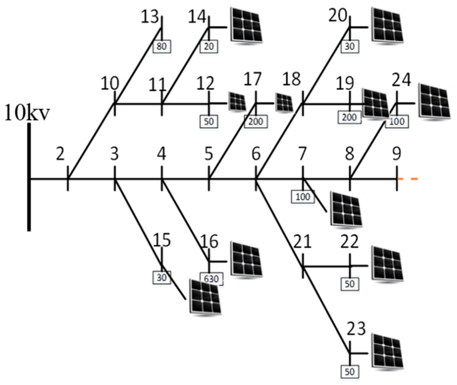
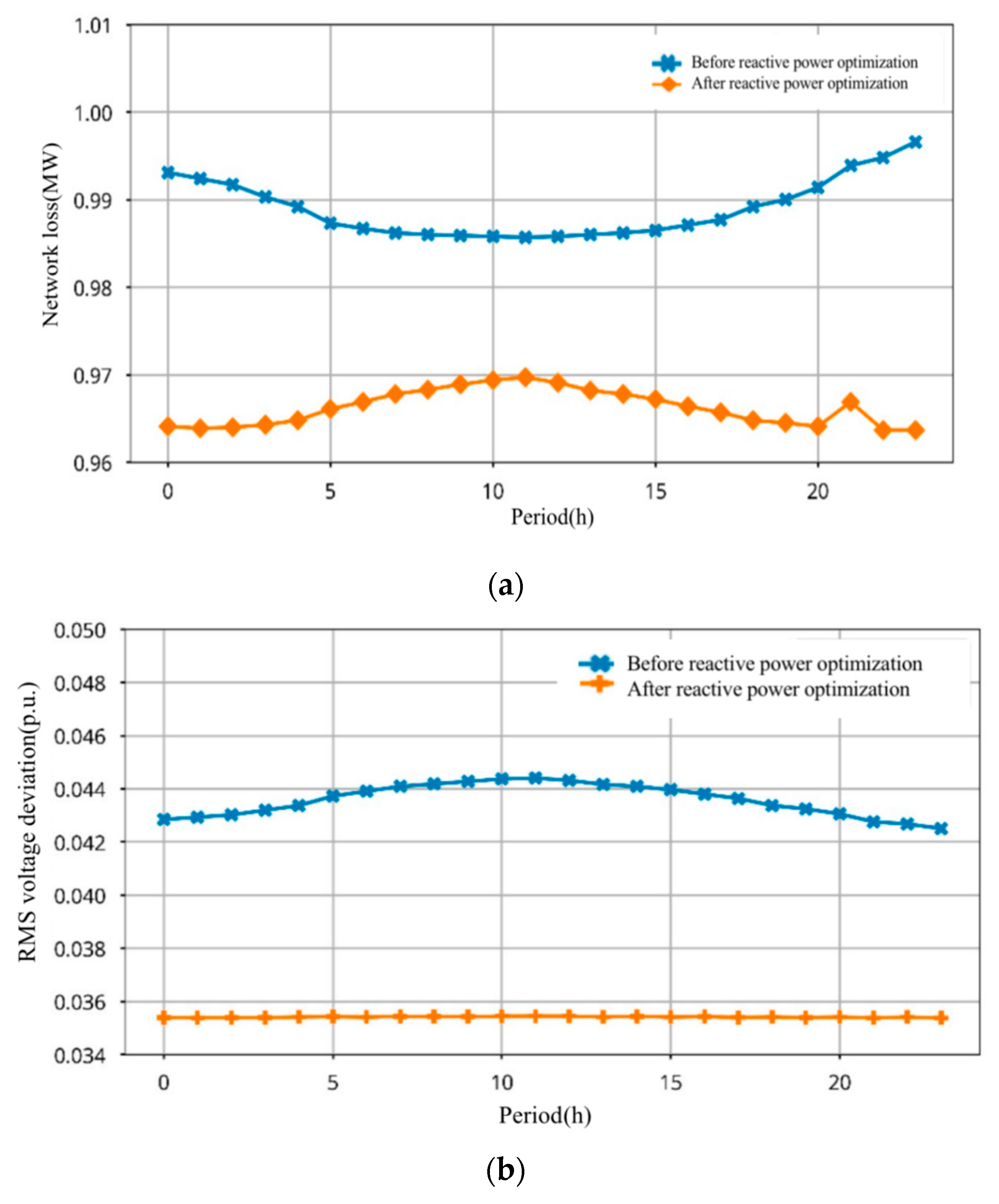
4.2. Simulation of Reactive Power and Voltage Control Model

Using a typical power system (shown in Figure 5) as a case study, we conducted a 24 h active power–reactive power coordination optimization study between the main grid and VPPs, utilizing the reactive power adjustment capability of the power plant as an adjustable resource. The system we used has 24 nodes as shown in Figure 5. The aim was to minimize the grid loss and average voltage deviations. By optimizing the adjustable resources among the VPPs collaboratively, grid loss and voltage deviations were reduced, and the voltage distribution was improved. The corresponding grid loss and voltage comparison before and after the optimization are shown in Figure 6.

5. Analysis of the Impact of the DER

This section studies the influence of the DER clusters on the grid. First, in the case of many DER clusters being injected into the grid, if the VPPs and the main grid are lacking in synergy, there will be a power flow reversal and voltage overload. Then, a robust optimal power flow model is utilized with the uncertainties of the DERs being considered to give strategies with better comprehensive economic benefits in different scenarios.

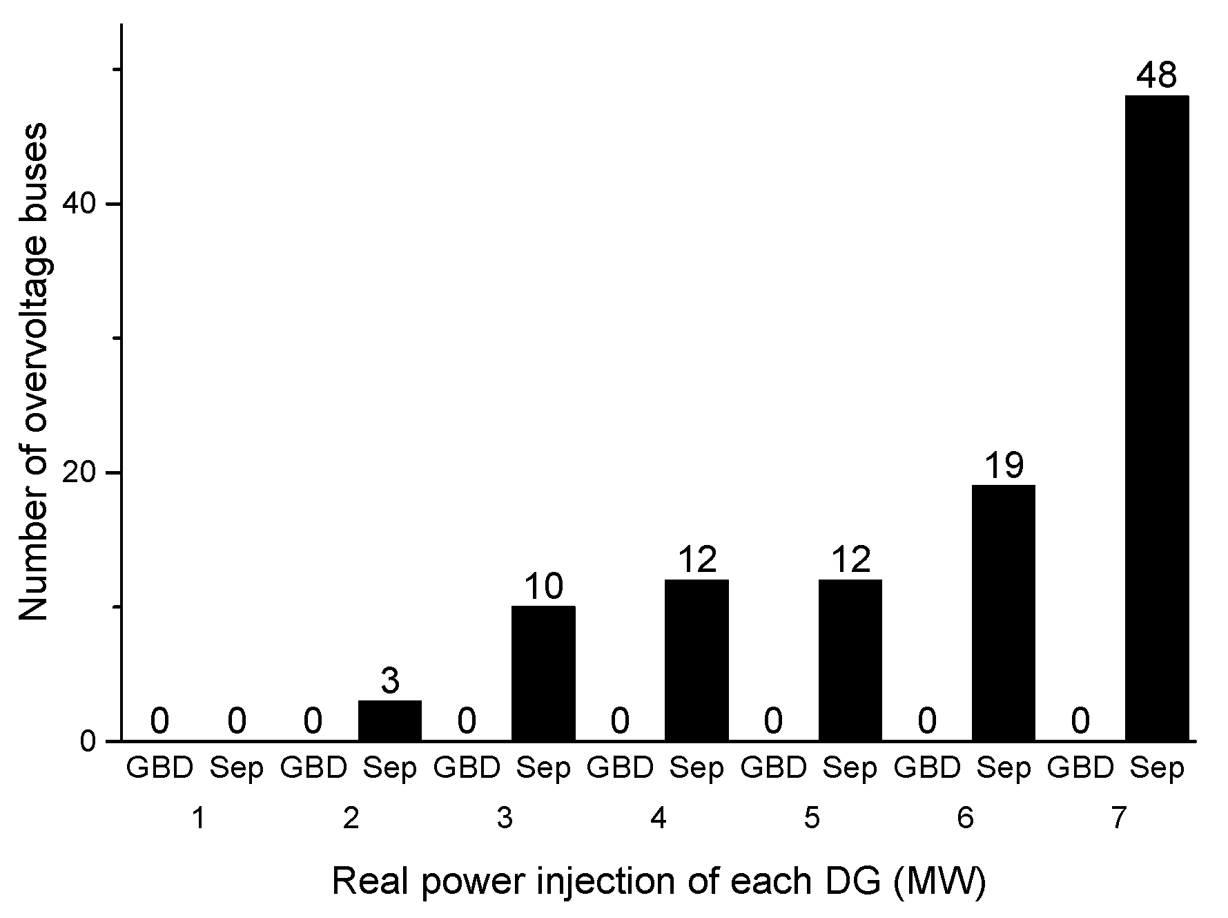
5.1. Impact of DER Clusters on Grid Voltage Security

Based on the generalized Benders decomposition, the proposed grid–VPPs reactive voltage optimization method (GBD) is compared with the independent algorithm (SEP). SEP is the current scheduling mode, that is, the voltage and transmission power of the boundary node are pre-set between the main grid and the VPP, and then each regional network is optimized, respectively. This method cannot obtain the global optimal solution, and sometimes there will be overvoltage problems.

Considering the power flow constraints in the VPP model (Constrains (25)–(28)), we can see that when a large number of DER clusters are connected to a node of a VPP, the node may appear to reverse the flow. A one-hundred-and-eighteen-node system is used as the main grid with three sixty-nine-node VPPs connected to nodes 54, 62, and 80, respectively. The boundary node of each VPP is node 1. DERs are located at nodes 3, 4, 8, 9, 11, 12, 27, 35, 39, 41, 54, 56, 58, and 69 of each VPP, with an adjustable reactive power range of [−50, 50] MVar.

Figure 7 shows the number of nodes whose voltage is higher thanthat of the third VPP as the output of the DERs increases. The proposed grid–VPP decomposition coordination algorithm can effectively eliminate the voltage overlimit problem through the iterative generation method of feasible cuts, while the traditional grid–VPP independent scheduling method can cause a serious voltage overshoot.

5.2. Influence of DERs Uncertainty on Power Grid Operation

Three scenarios are examined in this part: (a) the actual output of DER is at its lower bound; (b) the actual output of DER is at its predicted value; and (c) the actual output of DER is at its upper bound. The comparison results are as follows.

From the

Table 3. Comparison of total power generation costs under different scenarios.

		Scene a	Scene b	Scene c
System 1	Robust model	95,182	92,299	90,379
	Deterministic Model	94,627	94,627	94,627
System 2	Robust model	274,196	226,836	195,434
	Deterministic model	261,352	261,352	261,352

, we can observe that the robust optimal power flow model effectively diminishes the aggregate generation cost in Scene b and c through an affine adjustment strategy.

6. Conclusions

This paper introduced an interactive and coordinated optimization control method between VPPs and the main grid. The proposed method considered the VPP operation of multiple time scales, including intra-day and day-ahead. To address intra-day and day-ahead scheduling, a decomposed, coordinated and interactive method was provided, which was based on the multi-parametric programming projection decomposition method and generated the exact critical domain and the optimal cost function of the VPP internal scheduling model, which could significantly improve the convergence speed and stability compared with the existing decomposition and coordination algorithms. In terms of the reactive power and voltage control, the goal was to decrease the total loss of the VPPs and the main grid. The test results showed that the proposed method could quickly converge to the global optimal solution. In addition, the reactive power optimization method of VPPs–grid coordination could significantly reduce the overvoltage problem caused by the large number of DERs in the VPPs. Overall, this approach can efficaciously reduce the cost of the power grid and VPPs with fast convergence rates while also minimizing the system loss and voltage deviation to improve the voltage profile.

References

1. Akorede, M.F.; Hizam, H.; Pouresmaeil, E. Distributed energy resources and benefits to the environment. Renew. Sustain. Energy Rev. 2010, 14, 724–734. [Google Scholar] [CrossRef]
2. Huang, J.; Jiang, C.; Xu, R. A review on distributed energy resources and MicroGrid. Renew. Sustain. Energy Rev. 2008, 12, 2472–2483. [Google Scholar]
3. Spiller, E.; Esparza, R.; Mohlin, K. The role of electricity tariff design in distributed energy resource deployment. Energy Econ. 2023, 120, 106500. [Google Scholar] [CrossRef]
4. Strbac, G.; Jenkins, N.; Green, T.; Pudjianto, D. Review of innovative network concepts. In DG-GRID Project Report; Energy Research Centre of the Netherlands (ECN): Petten, The Netherlands, 2006. [Google Scholar]
5. Zhang, Y.; Pan, W.; Lou, X.; Yu, J.; Wang, J. Operation characteristics of virtual power plant and function design of operation management platform under emerging power system. In Proceedings of the 2021 International Conference on Power System Technology (POWERCON), Haikou, China, 10–11 November 2021; pp. 194–196. [Google Scholar] [CrossRef]
6. Ruiz, N.; Cobelo, I.; Oyarzabal, J. A direct load control model for virtual power plant management. IEEE Trans. Power Syst. 2009, 24, 959–966. [Google Scholar] [CrossRef]
7. Coelho, A.; Iria, J.; Soares, F. Network-secure bidding optimization of aggregators of multi-energy systems in electricity, gas, and carbon markets. Appl. Energy 2021, 301, 117460. [Google Scholar] [CrossRef]
8. Iria, J.; Scott, P.; Attarha, A.; Gordon, D.; Franklin, E. MV-LV network-secure bidding optimisation of an aggregator of prosumers in real-time energy and reserve markets. Energy 2022, 242, 122962. [Google Scholar] [CrossRef]
9. Fonseca, N.S.; Soares, F.; Coelho, A.; Iria, J. DSO framework to handle high participation of DER in electricity markets. In Proceedings of the 2023 19th International Conference on the European Energy Market (EEM), Lappeenranta, Finland, 6–8 June 2023; pp. 1–6. [Google Scholar] [CrossRef]
10. Gholami, K.; Azizivahed, A.; Arefi, A.; Li, L. Risk-averse Volt-VAr management scheme to coordinate distributed energy resources with demand response program. Int. J. Electr. Power Energy Syst. 2023, 146, 108761. [Google Scholar] [CrossRef]
11. Zhang, Y.; Yuan, F.; Zhai, H.; Song, C.; Poursoleiman, R. Optimizing the planning of distributed generation resources and storages in the virtual power plant, considering load uncertainty. J. Clean. Prod. 2023, 387, 135868. [Google Scholar] [CrossRef]
12. Danish, M.S.S.; Senjyu, T.; Nazari, M.; Zaheb, H.; Nassor, T.S.; Danish, S.M.S.; Karimy, H. Smart and sustainable building appraisal. J. Sustain. Energy Revolut. 2021, 2, 1–5. [Google Scholar] [CrossRef]
13. Himeur, Y.; Elnour, M.; Fadli, F.; Meskin, N.; Petri, I.; Rezgui, Y.; Bensaali, F.; Amira, A. Next-generation energy systems for sustainable smart cities: Roles of transfer learning. Sustain. Cities Soc. 2022, 85, 104059. [Google Scholar] [CrossRef]
14. Chen, J.; Deng, G.; Zhang, L.; Ahmadpour, A. Demand side energy management for smart homes using a novel learning technique–economic analysis aspects. Sustain. Energy Technol. Assess. 2022, 52, 102023. [Google Scholar] [CrossRef]
15. Wang, W.; Liu, H.; Ji, Y.; Qu, X. Optimal scheduling strategy for virtual power plant considering voltage control. In Proceedings of the 2021 International Conference on Power System Technology (POWERCON), Haikou, China, 14–16 September 2021; pp. 870–874. [Google Scholar] [CrossRef]
16. Vale, Z.; Pinto, T.; Morais, H.; Praça, I.; Faria, P. Virtual power plant’s multi-level negotiation in smart grids and competitive electricity markets. In Proceedings of the 2011 IEEE Power and Energy Society General Meeting, Detroit, MI, USA, 22 February 2011; pp. 1–8. [Google Scholar] [CrossRef]
17. Bertram, R.; Schnettler, A. A control model of virtual power plant with reactive power supply for small signal system stability studies. In Proceedings of the 2017 IEEE Manchester PowerTech, Manchester, UK, 18–22 June 2017; pp. 1–6. [Google Scholar] [CrossRef]
18. Ruthe, S.; Rehtanz, C.; Lehnhoff, S. Towards frequency control with large scale virtual power plants. In Proceedings of the 2012 3rd IEEE PES Innovative Smart Grid Technologies Europe (ISGT Europe), Berlin, Germany, 14–17 October 2012; pp. 1–6. [Google Scholar] [CrossRef]
19. Bao, Y.; Cheng, X.; Pi, J.; Zhang, Y.; Hou, C.; Guo, Y. Selection strategy of virtual power plant members considering power grid security and economics of virtual power plant. In Proceedings of the 2021 IEEE 5th Conference on Energy Internet and Energy System Integration (EI2), Taiyuan, China, 22–24 October 2021; pp. 1314–1319. [Google Scholar] [CrossRef]
20. Vasirani, M.; Kota, R.; Cavalcante, R.L.G.; Ossowski, S.; Jennings, N.R. An agent-based approach to virtual power plants of wind power generators and electric vehicles. IEEE Trans. Smart Grid 2013, 4, 1314–1322. [Google Scholar] [CrossRef] [Green Version]
21. Zhu, J.; Duan, P.; Liu, M.; Xia, Y.; Guo, Y.; Mo, X. Bi-level real-time economic dispatch of virtual power plant considering uncertainty of renewable energy sources. IEEE Access 2019, 7, 15282–15291. [Google Scholar] [CrossRef]
22. Giuntoli, M.; Poli, D. Optimized thermal and electrical scheduling of a large scale virtual power plant in the presence of energy storages. IEEE Trans. Smart Grid 2013, 4, 942–955. [Google Scholar] [CrossRef]
23. Alanne, K.; Saari, A. Distributed energy generation and sustainable development. Renew. Sust. Energ. Rev. 2006, 10, 539–558. [Google Scholar] [CrossRef]
24. Wang, Q.; Zhang, C.; Ding, Y.; Xydis, G.; Wang, J.; Østergaard, J. Review of real-time electricity markets for integrating distributed energy resources and demand response. Appl. Energy 2015, 138, 695–706. [Google Scholar] [CrossRef]
25. Järventausta, P.; Repo, S.; Rautiainen, A.; Partanen, J. Smart grid power system control in distributed generation environment. Annu. Rev. Control 2010, 34, 277–286. [Google Scholar] [CrossRef]
26. Mohd, A.; Ortjohann, E.; Schmelter, A.; Hamsic, N.; Morton, D. Challenges in integrating distributed energy storage systems into future smart grid. In Proceedings of the 2008 IEEE International Symposium on Industrial Electronics, Orlando, FL, USA, 30 June–2 July 2008; pp. 1627–1632. [Google Scholar]
27. Lin, C.; Wu, W.; Chen, X.; Zheng, W. Decentralized dynamic economic dispatch for integrated transmission and active distribution networks using multi-parametric programming. IEEE Trans. Smart Grid 2018, 9, 4983–4993. [Google Scholar] [CrossRef]
28. Lin, C.; Wu, W.; Zhang, B.; Wang, B.; Zheng, W.; Li, Z. Decentralized reactive power optimization method for transmission and distribution networks accommodating large-scale DG integration. IEEE Trans. Sustain. Energy 2017, 8, 363–373. [Google Scholar] [CrossRef]
Figure 1. The control framework of coordination between VPPs and the main grid.
Energies 16 05593 g001
Figure 2. A schematic of the main grid–VPPs coordination.
Energies 16 05593 g002
Figure 3. Equivalence of tie lines between VPPs.
Energies 16 05593 g003
Figure 4. Test system structure.
Energies 16 05593 g004
Figure 5. The topology of the typical power system.
Energies 16 05593 g005
Figure 6. (a) Comparison of grid loss before and after optimization. (b) Voltage comparison before and after optimization.
Energies 16 05593 g006
Figure 7. Test results of the voltage limit calculation example.
Energies 16 05593 g007