Article

Precise Dynamic Modelling of Real-World Hybrid Solar-Hydrogen Energy Systems for Grid-Connected Buildings

1
School of Engineering, Robert Gordon University, Aberdeen AB10 7GJ, UK
2
Department of Electrical and Control Engineering, College of Engineering and Technology, Arab Academy for Science, Technology and Maritime Transport, Alexandria P.O. Box 1029, Egypt
3
School of Computing, Engineering and the Built Environment, Edinburgh Napier University, Edinburgh EH10 5DT, UK
*
Author to whom correspondence should be addressed.
Energies 2023, 16(14), 5449; https://doi.org/10.3390/en16145449
Submission received: 14 June 2023 / Revised: 11 July 2023 / Accepted: 13 July 2023 / Published: 18 July 2023
(This article belongs to the Special Issue Advances on Solar Energy Materials and Solar Cells)

Abstract

:
Hybrid renewable hydrogen energy systems could play a key role in delivering sustainable solutions for enabling the Net Zero ambition; however, the lack of exact computational modelling tools for sizing the integrated system components and simulating their real-world dynamic behaviour remains a key technical challenge against their widespread adoption. This paper addresses this challenge by developing a precise dynamic model that allows sizing the rated capacity of the hybrid system components and accurately simulating their real-world dynamic behaviour while considering effective energy management between the grid-integrated system components to ensure that the maximum possible proportion of energy demand is supplied from clean sources rather than the grid. The proposed hybrid system components involve a solar PV system, electrolyser, pressurised hydrogen storage tank and fuel cell. The developed hybrid system model incorporates a set of mathematical models for the individual system components. The developed precise dynamic model allows identifying the electrolyser’s real-world hydrogen production levels in response to the input intermittent solar energy production while also simulating the electrochemical behaviour of the fuel cell and precisely quantifying its real-world output power and hydrogen consumption in response to load demand variations. Using a university campus case study building in Scotland, the effectiveness of the developed model has been assessed by benchmarking comparison between its results versus those obtained from a generic model in which the electrochemical characteristics of the electrolyser and fuel cell systems were not taken into consideration. Results from this comparison have demonstrated the potential of the developed model in simulating the real-world dynamic operation of hybrid solar hydrogen energy systems for grid-connected buildings while sizing the exact capacity of system components, avoiding oversizing associated with underutilisation costs and inaccurate simulation.

1. Introduction

Increased energy security and global warming concerns have led to tremendous change in the global energy mix, moving towards more localised renewable generation while reducing the reliance on imported fossil fuels. According to BP’s 2023 Energy Outlook [1], the renewables’ share from the global energy mix is expected to increase up to 65% by 2050, with fossil fuel resources falling to 20–50% from the global market share. To allow the integration of more renewables and help decarbonise the energy supply sector, there is an increasing need to store the surplus of renewable power generation for backup usage to secure energy demands. State-of-the-art hydrogen energy storage technologies have been identified as clean, sustainable solutions to achieve this aim, being at the forefront of the Net Zero carbon pathways. Renewable hydrogen energy systems can be used to absorb the excess of renewable power generation via water electrolysis and then feed it back as electricity when needed using fuel cell technologies, thus compensating for the renewables’ intermittency while accelerating the clean energy transition.
A key challenge facing the implementation of renewable hydrogen energy systems is the ability to precisely quantify the hydrogen production levels of an electrolyser when powered by a renewable energy source, as well as the hydrogen consumption levels and output power generation of a fuel cell when operating in response to load demand. While several models [2,3,4,5] are available in the literature for modelling the operating performance of electrolysis and fuel cell technologies, a research gap exists in modelling the dynamic operation of an entire hybrid renewable hydrogen energy system for backup power applications. When coupled with renewable energy, a real-world electrolyser will be operated under variable power levels in response to the intermittent nature of a renewable energy source, thus affecting the efficiency at which a hydrogen quantity can be produced. Similarly, when a real-world fuel cell is operating in response to variable load demand requirements, the electrochemical characteristics taking place inside the fuel cell will affect the output power being generated and thus the amount of hydrogen being consumed. This will then have a direct impact on the exact sizing of the hydrogen storage system required to avoid extra storage capacities following a complete cycle of filling and discharging this on-demand hydrogen fuel. Within the context of sizing and energy management of renewable hydrogen energy systems, recent research studies [6,7,8,9] have developed mathematical models for sizing and modelling the operation of hydrogen storage elements from techno-economic prospects of minimising the overall system cost while ensuring energy balance between generation and consumption. However, none of these has considered the electrochemical behaviour of electrolysers and fuel cell systems at variable power levels. This represents a significant deviation from simulating real-world renewable hydrogen energy systems and identifying realistic opportunities for decarbonising different sectors. In addition to the mathematical models developed, different computational modelling tools for simulating the performance of hydrogen energy storage systems have also been documented [10]. However, few software tools were found to be capable of sizing and simulating the dynamic operation of hybrid renewable hydrogen energy systems. Among these tools, HOMER 2 software (from National Renewable Energy Laboratories (NREL)) has been commonly used by researchers in recent literature [11,12,13,14,15,16] for simulating and optimising hybrid renewable energy systems incorporating hydrogen storage facilities. However, this tool does not account for the changes in electrochemistry losses occurring in electrolysis and fuel cell stacks under variable loading conditions [3]. Therefore, this introduces a significant drawback in determining the actual amount of hydrogen production by electrolysis and output power generation by fuel cells within hybrid renewable hydrogen energy systems. More emphasised modelling of renewable hydrogen energy systems can be provided via HYDROGEMS software [17], lately integrated with the TRANSYS 16 simulation platform; however, it lacks a capacity sizing feature for the integrated system components [18].
It is then obvious that sizing and simulating the real-world operation of renewable hydrogen energy systems is still in a less-advanced state. To address this challenge, this paper develops a precise dynamic model for sizing and simulating real-world hybrid solar hydrogen energy systems (HSHESs) to reduce the carbon emissions of grid-connected buildings. The developed model enables sizing the rated capacity of the HSHES components and accurately simulating their real-world dynamic behaviour, while considering effective energy management between the grid-integrated system components to ensure the maximum possible proportion of energy demand is supplied from clean sources rather than the grid. A set of mathematical models were developed through this research to allow identifying the real-world hydrogen production levels from electrolysers in response to the intermittent solar energy powering it, while also simulating the electrochemical behaviour of fuel cells and precisely quantifying their real-world output power generation and hydrogen consumption levels in response to load demand requirements. Combining the developed individual system component mathematical models together with the employed energy management strategy has formed the basis of the HSHES dynamic model presented in this research. To demonstrate the effectiveness of the developed dynamic system model, it was implemented on a Scottish university campus building in the city of Aberdeen, and the results were compared to those obtained from a generic model in which the electrochemical behaviours of the electrolyser and fuel cell systems are not considered. Analysis of this comparison has highlighted the potential benefits of the developed model in simulating the real-world dynamic operation of renewable hydrogen energy systems and sizing the exact capacity of their system components compared to the oversized capacities obtained from a generic simulation model.

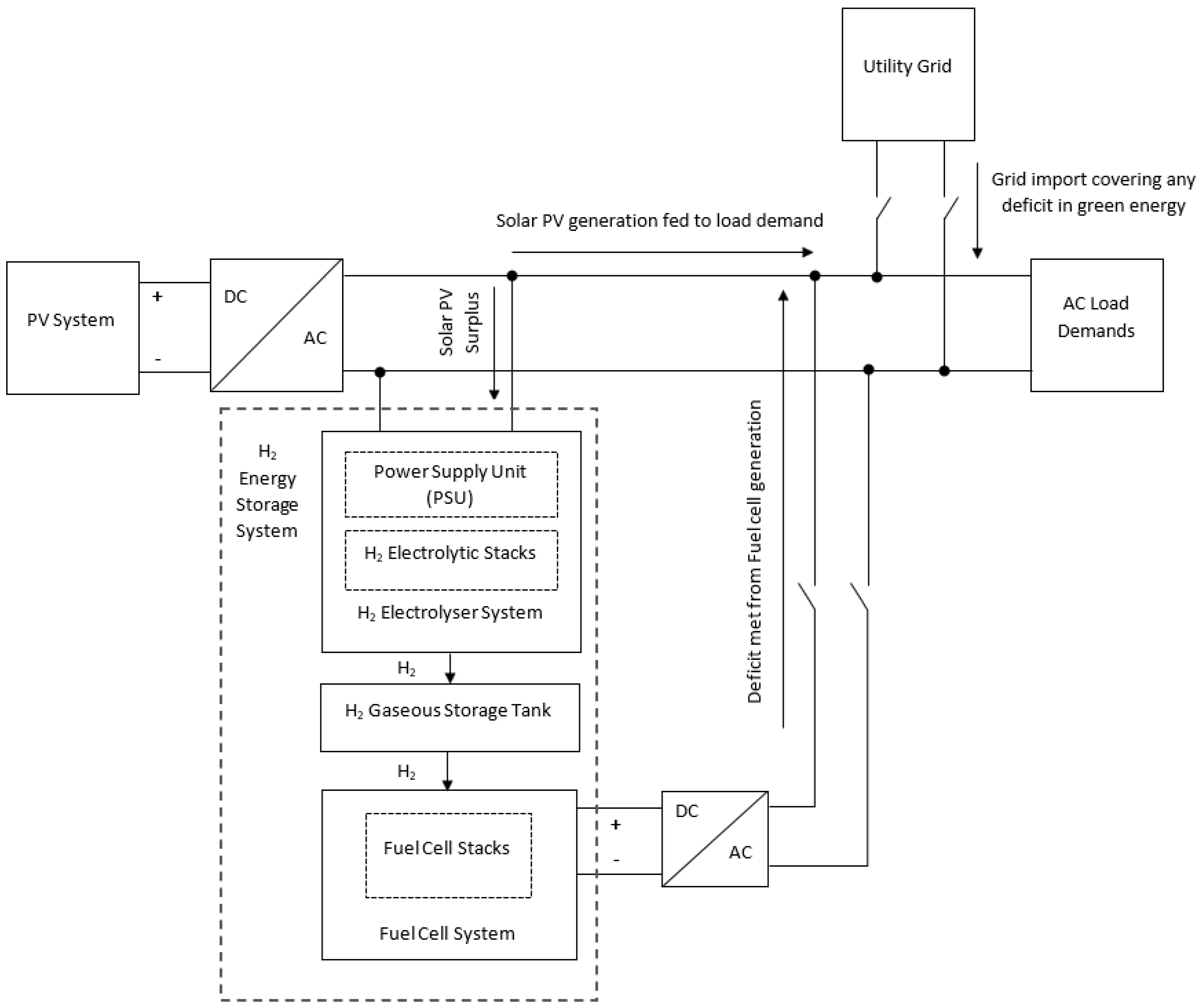
2. The Developed Model of Hybrid Solar-Hydrogen Energy System (HSHES)

The proposed HSHES is composed of a solar PV system, water electrolyser, gaseous hydrogen storage tank and fuel cell facility. Figure 1 shows the schematic diagram developed for the proposed HSHES. As can be seen from Figure 1, the outgoings from the PV system and fuel cell facility are connected to DC/AC inverters as auxiliary components for serving the AC load demands. In this configuration, the load demands are primarily fed by the combination of PV system and fuel cell facility. Using the excess of PV generation, the electrolyser is powered to produce renewable hydrogen, which is subsequentially stored in a pressurised hydrogen storage tank for backup usage. The stored hydrogen gas is then converted into electrical power by the fuel cell for feeding the load demands during the hours of deficiency in PV generation. To maintain energy balance between generation and consumption, the utility grid is only allowed to take place to cover any remaining loads unsatisfied by the renewable energy production from PV and fuel cell facilities. In this way, the proposed hybrid configuration can ensure the security of energy demands and the power system operation reliability while increasing the clean energy supply and reducing grid energy purchase requirements. The developed model of the proposed HSHES involved a set of mathematical models for sizing and modelling the integrated system components and their dynamic interaction with each other under the considered energy management strategy. Details of the developed mathematical models are given in the following subsections. More clarification regarding the mathematical equations used in developing these models can be found in Appendix A.

2.1. PV System Model

The solar PV system represents the main power source feeding the load demands during hours of high solar power availability. The first step in modelling the operation of the proposed hybrid system involves sizing the rated capacity of solar PV arrays, considering the capacity factor of the proposed PV system. In practice, PV capacity factors are highly dependent on the geographical location where the PV system is planned to be installed due to variations in weather conditions. Given that PV arrays are rated by manufacturers with a reference value of solar irradiation at standard test conditions (1000 W/m2), it is then possible to estimate the capacity factor of the proposed PV system using actual data of solar irradiation over a given period at the location the PV system is going to be installed. The fraction of average actual solar irradiation at the PV installation site to the reference value undertaken by manufacturers can then be used to estimate the PV capacity factor [18]. With the PV capacity factor determined, the installed capacity of the proposed PV system can be calculated using Equation (1), where the sized PV capacity average output power should be at least enough to supply the average power demand. As the surplus in PV production will be utilised to generate green hydrogen by electrolysis during hours of high PV production, it is then essential to compute the output power from the sized PV capacity at a particular time step. This mainly depends on actual values of solar irradiation and ambient temperature at the given time step to account for losses in PV arrays. For accuracy, a one-hour time step is considered in this model to account for variations in atmospheric conditions over a one-year timescale. The hourly output power from the sized PV capacity can then be calculated using Equations (2) and (3), as a function of hourly solar irradiation and PV cell temperature at the PV installation site [6,7].
P P V = P P V a v g C F P V
P P V t = P P V × G ( t ) G S T C 1 + K t × T C ( t ) T S T C
T C t = T a m b t + N O C T T N O C T × G S T C G N O C T
where
P P V Installed capacity of the proposed PV system
P P V a v g Average output power of the sized PV capacity
C F P V PV capacity factor
P P V t The hourly output power from the sized PV capacity
T a m b t The hourly ambient temperature at the PV installation site
T C ( t ) The hourly PV cell temperature at the PV installation site
G ( t ) The hourly solar irradiation at the PV installation site
G S T C Solar irradiation in standard test conditions (1000 W/m2)
T S T C PV cell temperature in standard test conditions (25 °C)
N O C T Nominal operating cell temperature (46 °C)
T N O C T Ambient temperature at which defined NOTC (20 °C)
G N O C T Solar irradiation at which defined NOTC (800 W/m2)
K t Temperature coefficient of power (−0.38%/°C)
As can be seen from Figure 1, the outgoing from the sized PV system is connected to DC/AC inverter for serving the AC load demands. Solar PV inverters are often highly efficient with standard rated efficiencies reaching up to 96% based on the inverter model and materials [19]. Considering a 90% inverter efficiency, the hourly output power at the outgoing of the PV inverter could be calculated using Equation (4). The hourly power served to the load from the sized PV system could then be identified using Equation (5).
P P V i n v t = P P V ( t ) × η i n v
P P V l ( t ) = P P V i n v t , P P V i n v t P l ( t ) P l ( t ) , P P V i n v t > P l ( t )
where P P V i n v t is the hourly output power at the outgoing of the PV inverter, P P V l ( t ) is the hourly power served to the load from the sized PV system, P l ( t ) is the hourly actual load demand, and η i n v is the PV inverter efficiency.

2.2. Electrolyser Model

In order to appropriately size the electrolyser to absorb the surplus in PV generation, it is essential to compute the power mismatch taking place between the hourly output power at the outgoing of the PV inverter and the hourly actual power demand during hours of PV surplus power generation. Identifying the maximum power mismatch occurring throughout the considered time interval then yields the maximum PV surplus power resulting from the sized PV capacity due to the time shift between hours of peak solar energy generation and hours of peak energy demand. In terms of cost-effectiveness, it is recommended to operate electrolysers at higher utilisation rates to compensate for their associated high capital expenditures, particularly when the maximum PV surplus power is unlikely to frequently occur over the considered time. To account for the level of underutilisation of the proposed electrolyser during hours of deficit in PV production, a reduction in the maximum PV surplus power is undertaken in this model [18], to size the capacity of the proposed electrolyser as given by Equation (6). It should be noted that the closest standard capacity to this value is taken into consideration when sizing the electrolyser based on a conducted market survey of commercially available electrolyser products. The downside of this method is that there will be time periods where the PV excess production surpasses the rated power that the sized electrolyser can absorb.
Given that the proposed electrolyser will be operated at variable power levels in response to the excess in PV production, the electrolyser is then allowed to absorb the hourly PV surplus power if this is less than or equal to the sized capacity of the proposed electrolyser as given by Equation (8). If the PV surplus power exceeds the sized capacity of the electrolyser, then the hourly power absorbed by the electrolyser is set equivalent to its sized capacity and the remainder accounts for non-utilised PV excess as given by Equation (9).
P e l e = m a x . [ P t ] 2
P t = P P V i n v ( t ) P l ( t ) , P P V i n v ( t ) > P l ( t )
P e l e t = P t , P ( t ) P e l e P e l e , P ( t ) > P e l e
P e x P V t = P t P e l e t , P ( t ) > P e l e
where P e l e is the rated capacity of the proposed electrolyser, P t is the hourly PV surplus power, P e l e t is the hourly power absorbed by the electrolyser, P e x P V t is the hourly non-utilised PV excess, and m a x is the maximum value of hourly PV surplus power identified over the considered time interval.
To simulate the output of a real-world electrolyser running back renewable energy source, there is a need to develop an accurate dynamic model to account for variations in hydrogen production levels under electrolyser variable loading conditions. In general, the hydrogen quantity being generated by the electrolyser depends on the electric current flowing in the electrolytic cell [3]. Large-scale electrolysers are often comprised of smaller stacks connected in parallel to increase the output gas flow. Each electrolytic stack consists of several cells connected in series. Based on industry standards, the power supply unit (PSU) (with ac to dc converter) is internally integrated with the electrolytic stack as changes in the power supply output voltage are what controls the current density and therefore the ultimate gas production rate. Standard voltage ratings of electrolyser units in the MW scale are typically 400 V, 690 V or 11 kV, depending on the size of the machine. Considering a 400 V large-scale electrolyser unit for absorbing the excess in PV production and given that an electrolysis unit is formed of multiple electrolytic stacks connected in parallel, it is then possible to determine the hourly input current per electrolytic stack using the number of operational stacks and the total input current to the electrolyser unit. It should be noted that the number of electrolytic stacks that get into operation will vary according to the electrolyser operating point. The more power absorbed by the electrolyser, the higher the number of electrolytic stacks that get into operation to increase the output gas flow and vice versa. Given that smaller electrolytic stacks are stacked together to allow the absorption of hourly PV surplus power up to the sized capacity of the electrolyser, the number of operational stacks can then be identified by the selection of a commercially available electrolytic stack that will be used to build up the whole electrolyser unit.
In order to accurately quantify the hydrogen production levels by electrolysers at variable power consumption levels, Faraday efficiency is used. Faraday efficiency accounts for parasitic current losses occurring within the electrolytic cell stack due to gas crossover. In basic terms, this can be defined as the fraction of actual hydrogen quantity that could be produced by an electrolyser to the maximum theoretical quantity of hydrogen production [20]. The impact of Faradaic current losses on the rate of hydrogen production per electrolytic stack is modelled using Equation (10) [3]. The rate of hydrogen production per single cell is directly proportional to the electrons’ transfer rate at the electrodes, which depends on the electric current passing through the electrolytic cell. An empirical model [3] is then used in Equation (11) to account for variations in Faraday efficiency as a function of electrolysis current densities. With the proposed electrolyser running back the excess in intermittent PV production, Faradaic current losses will then vary with the electrical current passing through the electrolytic cell. It is then most importantly to account for hourly variations in the Faraday efficiency as more or less current is absorbed by the electrolyser. The total hydrogen quantity produced by the whole electrolyser consisting of multiple stacks can then be accordingly identified by means of the number of operational stacks as expressed in Equation (12).
n H 2 p ( t ) = η F ( t ) n c i e l e ( t ) z F
η F ( t ) = ( i e l e ( t ) / A ) 2 f 1 + ( i e l e ( t ) / A ) 2 f 2
m H 2 p t = n H 2 p × M × N e t × 3600
where
n H 2 p ( t ) The molar flow rate of hydrogen production per electrolytic stack (mol/s).
η F ( t ) Faraday efficiency at the value of current absorbed by the electrolytic cell.
i e l e ( t ) The input current per electrolytic cell.
m H 2 p t The hourly mass of total hydrogen production by the electrolyser unit (kg/h).
N e t Number of operational electrolytic stacks.
n c Number of cells per electrolytic stack.
M Molar mass of hydrogen gas ( 2.016 × 10 3 kg/mol).
z Number of electrons transferred per reaction (2).
F Faraday constant (96,485 C/mol).
A Electrode area (m2).
f 1 Parameter used in modelling the Faraday efficiency (mA2cm−4).
f 2 Performance coefficient whose value is empirically selected between 0 and 1.
The parameters f 1 and f 2 are two factors that have been introduced in the modelling equation of the Faraday efficiency for hydrogen production, whose values are empirically selected to help model the non-linear cell characteristic in such a way that best represents the real-world performance of an electrolytic cell.

2.3. Hydrogen Storage Tank and Fuel Cell Model

The size of the hydrogen storage tank depends on the hydrogen quantity being consumed by the fuel cell with this on-demand hydrogen fuel being continuously charged during peak sunlight hours and conversely discharged during night hours on a daily basis over the considered time interval. Therefore, the electrochemical characteristic of the fuel cell system is dynamically modelled in this work to accurately identify the output power generation and hydrogen consumption levels by the fuel cell in response to load demand requirements and accordingly indicate the maximum capacity of the hydrogen storage tank following the annual charging and discharging of hydrogen fuel.
The first criterion is to size the proposed fuel cell system. Given that the proposed fuel cell system will be operating to cover the deficit of PV production in supplying the load demand, the size of the fuel cell system should be at least enough to cover the maximum hourly deficit in load demand that can occur during hours of deficiency in PV production throughout the considered time interval. Accordingly, the maximum hourly deficit in load demands is identified over the year in this model to size the rated capacity of the fuel cell system as given by Equation (13). It should be noted that the closest standard capacity to this value is taken into consideration when sizing the fuel cell based on a conducted market survey of commercially available fuel cell products.
P F C = m a x . [ P d e f t ]
P d e f t = P l ( t ) P P V i n v ( t ) , P P V i n v t < P l ( t )
where P F C is the rated capacity of the proposed fuel cell system, P d e f t is the hourly deficit in load demand, and m a x is the maximum hourly deficit in load demand identified over the considered time interval.
In common with electrolysers, most fuel cell systems are composed of smaller stacks connected in parallel to increase the total output current, and each stack has several cells connected in series. To deliver accurate simulation results, the stack voltage model [18,21] is considered in this work to dynamically quantify the output power generation by the sized fuel cell system based on the hydrogen availability in the storage tank and load demand requirements while accounting for electrochemical losses occurring in fuel cell stacks. The basic reaction of a single fuel cell implies the transfer of two electrons per hydrogen mole. Therefore, the hydrogen consumption rate in a fuel cell stack consisting of several cells connected in a series is given by Equation (15) [21]. Using the hydrogen mass available in the storage tank, the hydrogen consumption molar flow rate per fuel cell stack can be identified given the hydrogen gas molar mass and the number of fuel cell stacks required to build up the sized capacity of the fuel cell system. The hydrogen mass available in the storage tank is given by Equations (16) and (17).
n H 2 c t = n f c i f c t 2 F
m H 2 a v t = m t a n k t 1
m t a n k t = m t a n k t 1 + m H 2 p t
where n H 2 c t is the hydrogen consumption molar flow rate per fuel cell stack (mol/s), n f c is the number of fuel cells per stack, i f c t is the fuel cell operating current (A), m H 2 a v t is the hydrogen mass available in the storage tank at time step (t) in kg/h, and m t a n k t is the hydrogen storage tank hourly mass status.
To identify the output power that the sized fuel cell system can deliver with the hydrogen available in the storage tank, it is essential to account for irreversible losses taking place inside the fuel cell. Each fuel cell experiences some losses due to fuel cell electric resistance, inefficiency of reactant gas transport and slow reactions taking place inside the cell [21]. These losses are often referred to as activation losses, ohmic losses and concentration losses [22]. The difference between the actual cell potential and the ideal (reversible) cell potential represents these losses as shown in Equation (18) [18,21].
U f c ( t ) = U r e v U a ( t ) U o ( t ) U c ( t )
where U f c ( t ) is the hourly actual fuel cell voltage, U r e v is the ideal (reversible) cell voltage, U a ( t ) is the hourly activation losses, U o ( t ) is the hourly ohmic losses and U c ( t ) is the hourly concentration losses.
The ideal or reversible cell voltage can be defined by the Nernst equation from the open circuit voltage of a fuel cell. The ideal cell voltage at the standard reference temperature of 25 °C (298 °K) for a fuel cell in which hydrogen and oxygen are gas reactants is 1.229 V [22]. However, the ideal cell voltage is highly affected by the cell temperature and the partial pressures (concentrations) of reactants, given that the reactant concentrations at the exit of the cell will be lower than those at the entrance, leading to a reduction in the ideal cell voltage [22]. This can be expressed by Nernst correction as shown in Equation (19) [21], to account for variations in cell temperature with respect to the standard reference value and the reduction in gas reactants concentrations.
U r e v = 1.229 0.85 × 10 3 × T 298.15 + 4.3085 × 10 5 T [ ln P h 2 + 1 2 ln P O 2 ]
where T is the fuel cell temperature in Kelvin (°K) and P h 2 and P O 2 are the partial pressures of hydrogen and oxygen gas reactants in Pascal (Pa), respectively.
The activation losses are caused by the activation energy required for slow electrochemical reactions to take place on the surface of the fuel cell electrodes. A small portion of the generated voltage is consumed in facilitating the transfer of electrons to and from the anode and cathode electrodes. The activation losses can be calculated using Equations (20) and (21) [18,21], as functions of the fuel cell operating current.
U a t = [ ξ 1 + ξ 2 T + ξ 3 T ln C O 2 + ξ 4 T ln i f c t ]
C O 2 = P O 2 5.08 × 10 6 × e ( 498 T )
where ξ 1 , ξ 2 , ξ 3 , a n d   ξ 4 are parametric coefficients of the fuel cell whose values are given by theoretical equations with kinetic, thermodynamic and electrochemical foundations, and C O 2 is the concentration of oxygen at the catalytic interface of the cathode (mol/C3).
The ohmic losses occur either due to internal current losses or resistive losses. Internal current losses occur when some electrons leak through the membrane instead of passing through the external circuit, while resistive losses result from electrons flowing through the resistance of the entire electric circuit. These losses are directly proportional to the current density. The ohmic losses can be found using Equations (22) and (23) [18], where the exponential term in Equation (23) represents the temperature correction in membrane resistivity if the cell is not operating at 30 °C (303 °K) [21].
U o t = i f c t [ ρ M ( t ) L A + R c ]
ρ M ( t ) = 181.6 1 + 0.03 i f c t A + 0.062 T 303 2 . i f c t A 2.5 λ 0.634 3 i f c t A . e x p [ 4.18 ( T 303 T ) ]
where ρ M ( t ) is the membrane resistivity in (Ω.cm), A is the membrane active area in (cm2), L is the membrane thickness in (cm), R c is the resistive coefficient in (Ω), T is the fuel cell temperature in degree Kelvin (°K), and λ is the humidification level of the membrane, describing the process of water by-product circulation throughout the membrane and its impact on the fuel cell performance. Dried membranes decrease the conductivity of protons while humid membranes may significantly increase the voltage losses. Thus, there should be a process of water management throughout the membrane to maintain a proper humidity level. The ideal state involves blowing air over the cathode to facilitate the water diffusion from the cathode to the anode and throughout the electrolyte, thus dehydrating any excess water and maintaining an appropriate humidity level. However, variations could occur during this process [21]. Thus, an adjustable design variable ( λ ) is introduced in Equation (23) to help model the impact of the membrane humidity level on the fuel cell performance ( λ = 14 at the ideal humidity state, λ = 23 at oversaturated states).
The concentration losses are due to variations in gas reactant concentrations at the electrode surfaces in each cell and are highly dependent on current densities. A drop in reactant concentrations is associated with an increased voltage drop, particularly at high current densities, meaning that concentration losses are more apparent at increased load operation when more deficit is required to be met by the sized fuel cell system during hours of low or no PV production. The concentration losses can be obtained using Equations (24) and (25) [18,21], as functions of the current density.
U c t = β   l n ( 1 j ( t ) j m a x )
j ( t ) = i f c t A
where β is the parametric coefficient measured in volts, j ( t ) is the hourly current density in (A/cm2), and j m a x is the maximum current density in (A/cm2).
With the hourly actual cell voltage determined, the hourly output voltage from the sized fuel cell system can be obtained as expressed in Equation (26) [4], given that the latter is formed of multiple stacks connected in parallel and each stack has several cells connected in series. The hourly DC output power that the fuel cell can deliver with hydrogen available in the storage tank can be calculated using Equation (27) given that the output current from the fuel cell system is determined based on the number of parallel fuel cell stacks used in building the sized capacity of the fuel cell system. With the fuel cell system connected to an inverter for serving the AC load demands as illustrated in Figure 1, the hourly equivalent AC output power that the sized fuel cell system can deliver to the load demands through the inverter can be calculated using Equation (28):
U f c o u t t = U f c t × n f c
P f c d c t = U f c o u t t × I f c o u t t
P f c a c t = P f c d c t × η i n v
where U f c o u t t and I f c o u t t are the hourly output voltage and hourly output current from the fuel cell system with the hydrogen available in the storage tank, respectively; P f c d c t is the hourly DC output power that the fuel cell system is capable to deliver with the hydrogen available in the storage tank; P f c a c t is the hourly output power that the sized fuel cell system can deliver to the load demands through the inverter; n f c is the number of fuel cells per stack; and η i n v is the inverter efficiency.
The output power of the sized fuel cell system is then controlled to only allow serving the load demand requirements during the PV supply deficit hours using Equations (29) and (30).
P f c l ( t ) = P d e f ( t ) , P d e f ( t ) P f c a c t P f c a c t , P d e f ( t ) > P f c a c t
P g r i d t = P d e f t P f c l t ,   P d e f ( t ) > P f c a c t
where P f c l t is the hourly power served to the load from the sized fuel cell system during hours of low or no PV production, and P g r i d t is the proportion of load deficit met from the utility grid if the deficit exceeds the hourly output power that the fuel cell system can deliver through the inverter.
The fuel cell hydrogen consumption levels in response to load demand requirements are then identified based on the power served to the load from the sized fuel cell system. In case the power served to the load from the fuel cell system is set equal to the load deficit, the mass of hydrogen required to be consumed will depend on the number of fuel cell stacks that get into operation to deliver this deficit. It should be noted that the fuel cell operating current and the molar flow rate of hydrogen consumption per fuel cell stack remain unchanged; only the number of operational stacks will vary according to the required output power. With the stacks connected in parallel, the output voltage from the sized fuel cell system remains constant independent of the number of operational stacks; thus, the new value of output current required to deliver this load deficit will be the only factor driving the required output power from the fuel cell system and, accordingly, the number of operational stacks. The hourly mass of hydrogen that is required to be consumed to deliver the deficit in load demand can then be calculated as given by Equation (31). In case the power served to the load from the fuel cell system is set equal to the output power that the fuel cell system can deliver through the inverter, the hourly mass of hydrogen required to be consumed is set equal to the hydrogen mass available in the storage tank. The hydrogen storage tank hourly mass status is then updated as given by Equation (32). Following the annual charging and discharging of this on-demand hydrogen fuel, the hydrogen storage tank is then sized enough to cover the maximum quantity of hydrogen accumulated in the storage tank throughout the year as given by Equation (33).
m H 2 c t = n H 2 c × M × N f c ( t ) × 3600 , P f c l t = P d e f ( t ) m H 2 a v t , P f c l t = P f c a c t
m t a n k t = m t a n k t 1 m H 2 c t
M t a n k = m a x . [ m t a n k t ]
where m H 2 c t is the hourly hydrogen mass being consumed by the sized fuel cell system in response to load demand requirements in kg/h, M is the hydrogen gas molar mass ( 2.016 × 10 3 kg/mol), N f c ( t ) is the number of operational fuel cell stacks, M t a n k is the storage capacity of the hydrogen storage tank in kg, and m a x is the maximum value of hydrogen mass accumulated in the storage tank throughout the year.
It should be noted that the closest higher standard capacity to this value is considered when sizing the hydrogen storage tank based on a conducted market survey of commercially available pressurised hydrogen storage vessels. The equivalent gas volume and target pressure of the hydrogen storage tank were accordingly identified based on the sized mass storage capacity.

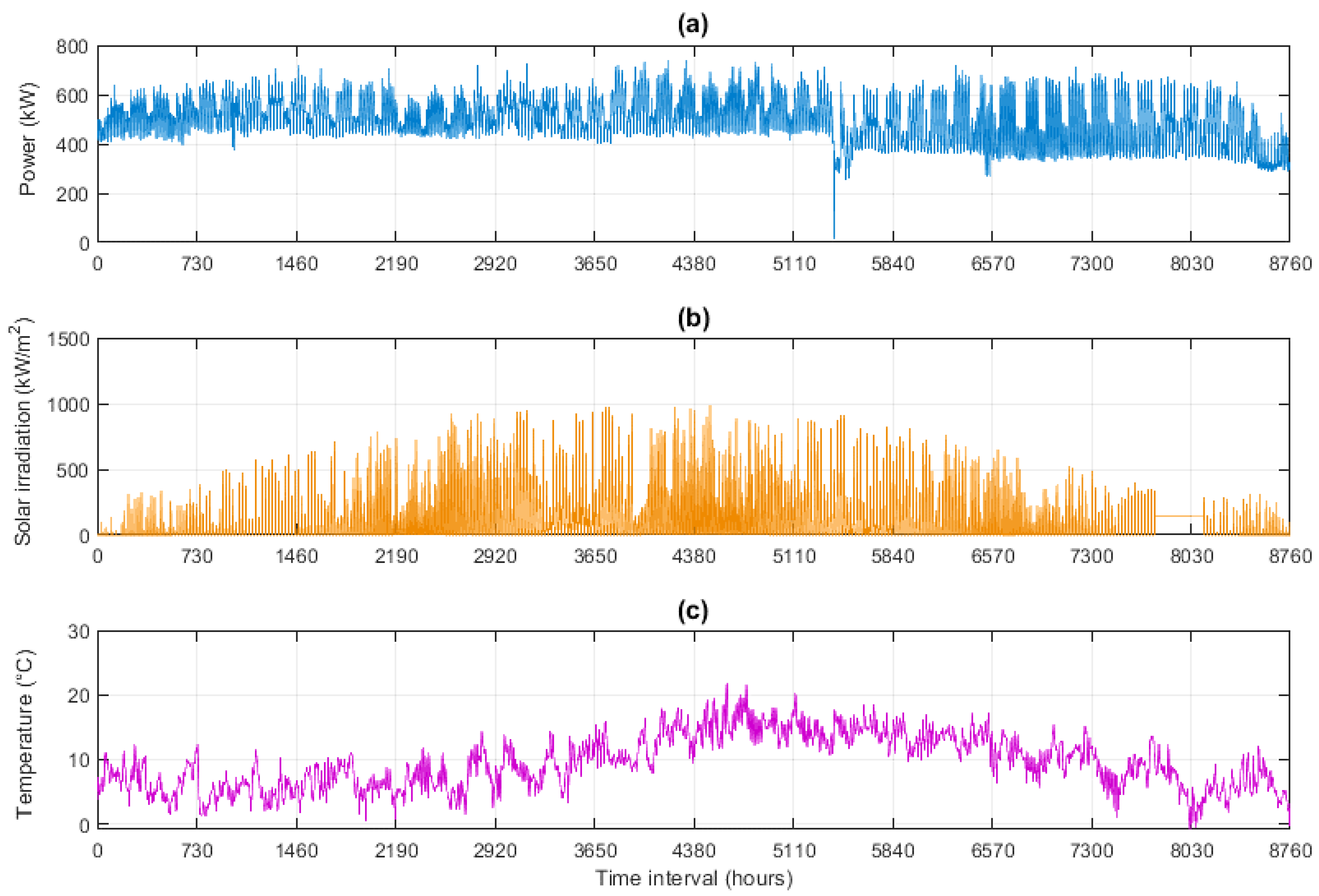
3. Case Study: The Sir Ian Wood Building—Robert Gordon University

The Robert Gordon University (RGU), an educational institution in Aberdeen city in Scotland, has recently initiated a commitment to Net Zero aiming to support the Scottish government’s goals in achieving the Net Zero ambition by 2045. In line with the university’s ongoing campaign to reduce its carbon footprint, the Sir Ian Wood Building (SIWB), one of the campus buildings with the largest energy needs, has been selected as a case study to implement the developed model for planning a realistic and successful building energy transition. Figure 2a shows the actual data of the hourly load demand profile collected for SIWB over a one-year time interval. The building annual energy demand is around 4356 MWh, with an average hourly power demand of 497.2 kW and peak hourly power demand of 738 kW. Figure 2b,c show the hourly data of solar irradiation and ambient temperature at the building location, respectively, over a one-year time interval. The illustrated data of atmospheric conditions are collected using the PVGIS web interface. From the data of hourly solar irradiation at the building location, the average hourly solar irradiation was found to be around 120 W/m2 and, accordingly, the PV capacity factor is estimated at approximately 12%. The parameters used in developing the electrolyser, hydrogen storage and fuel cell system models are given in Table 1 and Table 2, respectively, and they were extracted from [4,18], respectively.

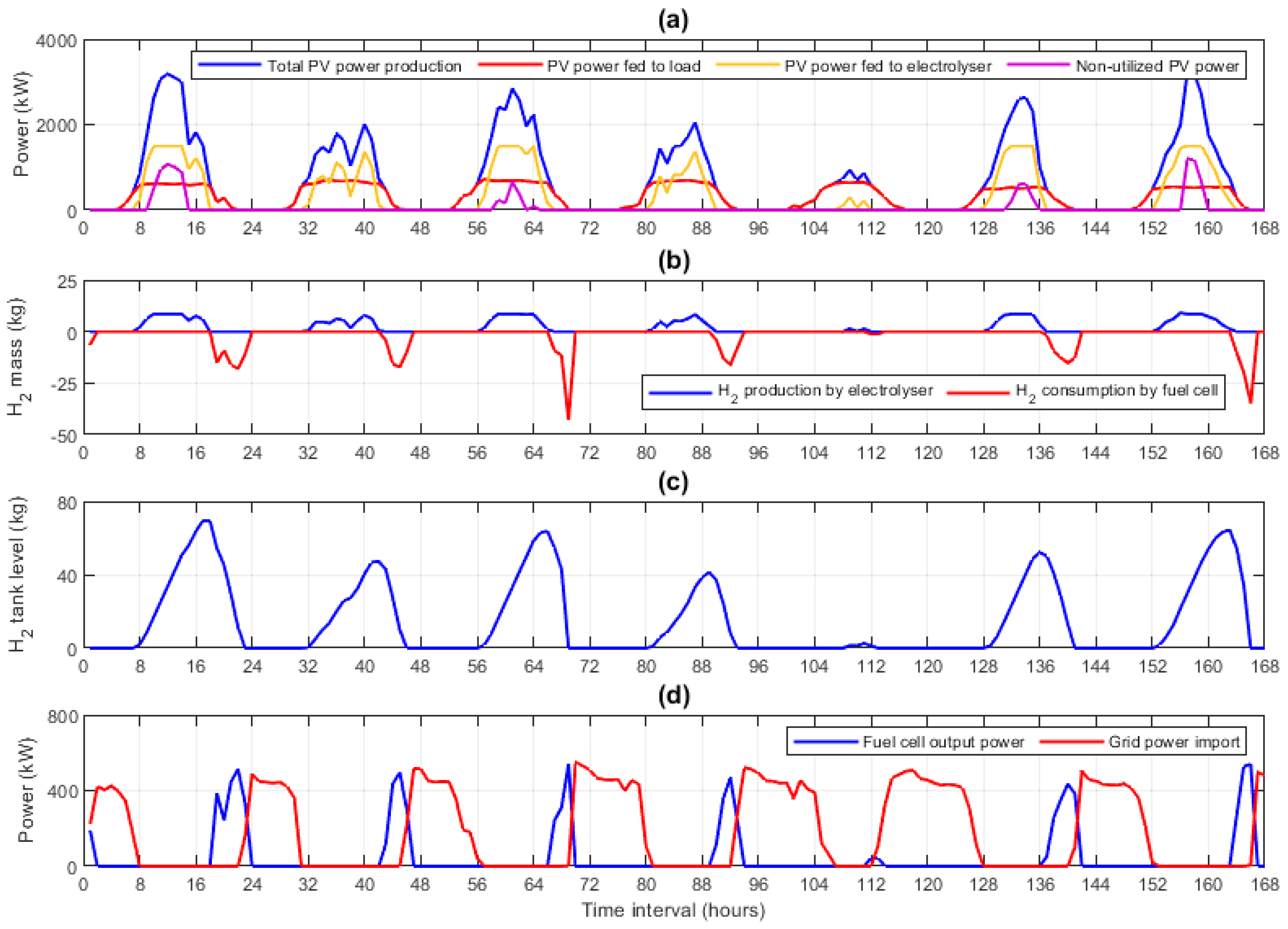
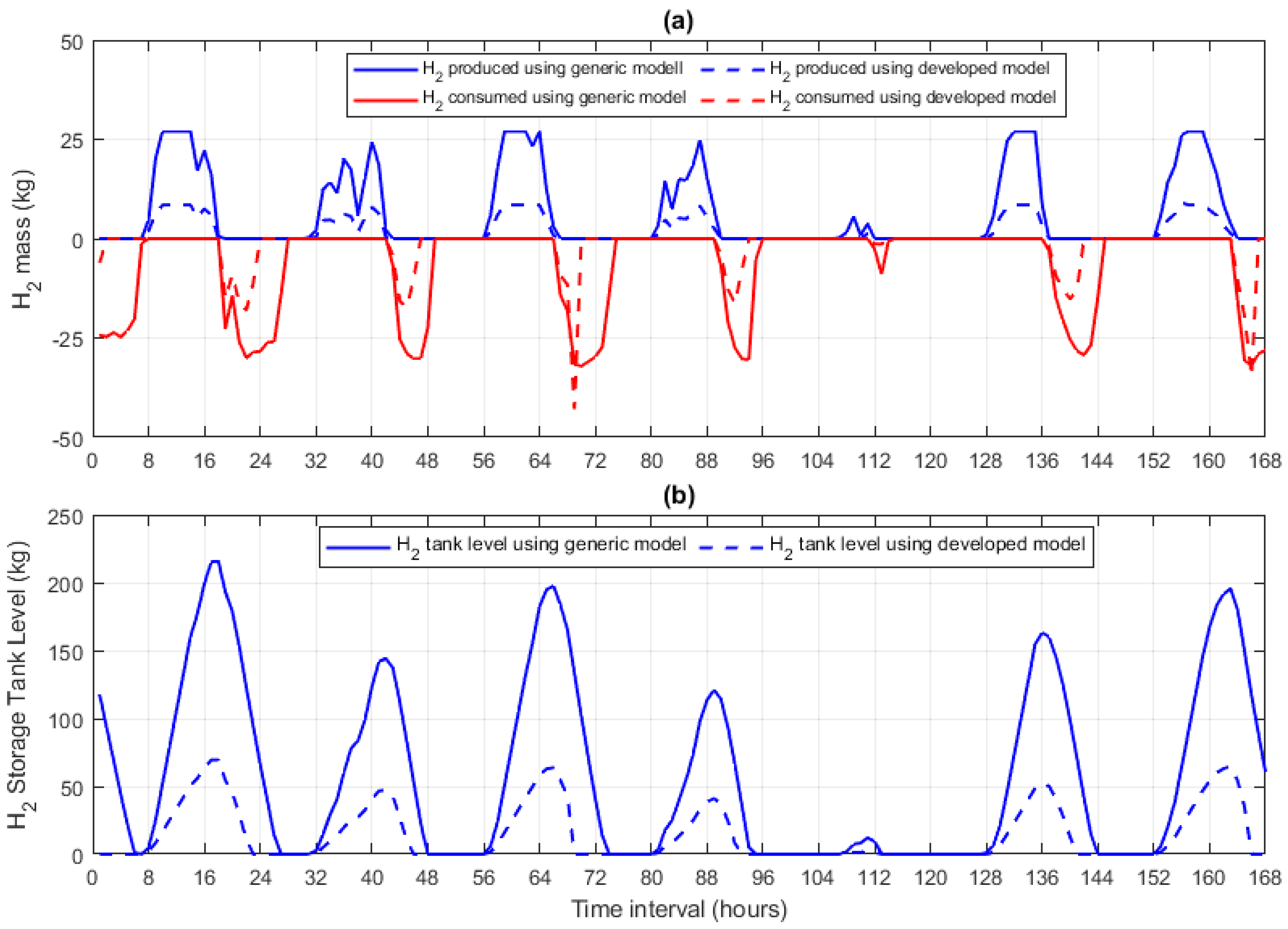
4. Results and Discussion

Table 3 shows the developed model sizing results for the HSHES suited for reducing SIWB carbon footprint. The sized hybrid system comprised a 4.15 MW PV capacity in conjunction with a 1.5 MW electrolyser unit, 600 kW fuel cell system and 106 kg of pressurised hydrogen storage tank to mitigate the intermittency of solar energy production. Figure 3a shows the sized PV system hourly simulation results over an exemplary period (one summer week). This includes the hourly total PV power production, the hourly PV power fed to load demand, the hourly PV power fed to the electrolyser and the hourly non-utilised PV power. Figure 3b shows the hourly hydrogen production levels by the electrolyser during the hours of PV surplus power generation and, conversely, the hourly hydrogen consumption levels by fuel cell during the hours of deficiency in PV generation over the same exemplary period. Consequently, Figure 3c shows the hourly hydrogen storage tank level over the same exemplary period, indicating that the storage tank is filling hydrogen during the hours of excess in PV generation while consuming the stored hydrogen during the hours of deficiency in PV generation. Figure 3d shows the fuel cell hourly output power generated during the hours of deficiency in PV generation, together with the hourly power imported from the utility grid over the same exemplary period. From the obtained results, it can be concluded that the sized electrolyser is operated at variable power levels in response to intermittent solar energy generation to store the PV surplus power as green hydrogen during the hours of excess in PV generation. In contrast, the sized fuel cell system, in conjunction with the utility grid, operates in response to load demand requirements during the hours of deficiency in PV generation, therefore maintaining a successful energy balance between the integrated system components while ensuring an increased proportion of green energy supply.
To evaluate the effectiveness of the developed model in quantifying the real-world hydrogen production levels by electrolysers when running back intermittent renewable energy sources while also identifying the real-world output power generation by fuel cells and their corresponding hydrogen consumption levels in response to variable load demand requirements, the developed model simulation results have been compared to those obtained from a generic model [23] in which the changes in electrochemical losses taking place inside the electrolysers and fuel cell stacks are not taken into consideration. For the purpose of comparison, the hourly operation of the integrated system components is simulated in both models using the same sized capacities listed in Table 3, together with the same PV system model included in Section 2.1. Figure 4a compares the hourly hydrogen production by the electrolyser and the hourly hydrogen consumption by the fuel cell obtained using the developed model versus those obtained using the generic model over the same exemplary period. The analysis of comparative results shows that lower hydrogen production levels are obtained from the electrolyser using the developed model compared to those obtained using the generic model. This shows the impact of accounting for hourly variations in Faradaic current losses on the molar flow rate of hydrogen production as more or less PV surplus power is absorbed by the electrolyser. Similarly, lower hydrogen quantities are seen consumed by the fuel cell using the developed model compared to those consumed using the generic model as a result of modelling the changes in the Faraday efficiency and their impact on the ultimate gas production rate resulting in less hydrogen availability in the storage tank within the developed model. Furthermore, modelling the electrochemical losses taking place inside the fuel cell and their impact on the output power generation that the fuel cell is capable to deliver has consequently lowered the equivalent hydrogen quantities being consumed by the fuel cell within the developed model. Figure 4b compares the hourly hydrogen storage tank level obtained using the developed model versus the one obtained using the generic model over the same exemplary period. As can be seen from Figure 4b, modelling the real-world dynamic behaviour of the sized HSHES within the developed model considering intermittency in solar energy production and variability of load demand has a great impact on reducing the hydrogen storage tank level attained using the developed model compared to the one attained using the generic model. From the simulation results of hourly hydrogen storage tank level over the whole year interval, the maximum level attained in the hydrogen storage tank was found to be 86.5 kg of hydrogen using the developed model, versus approx. 315 kg of hydrogen using the generic model, thus highlighting the potential benefits of the developed model in sizing the exact capacity of hydrogen storage systems, avoiding oversized storage capacities associated with additional costs and bulky space requirements.
Figure 5 compares the hourly fuel cell output power and hourly grid power import obtained using the developed model versus those obtained using the generic model over the same exemplary period. As can be seen from Figure 5a, the developed model simulation results show the sized fuel cell system serving the load demand for shorter time intervals compared to those illustrated by the generic model. This is due to less hydrogen availability in the storage tank obtained within the developed model as a result of precise dynamic modelling of the sized HSHES, thus restricting the operation of the fuel cell system for limited periods of time according to the real quantity of hydrogen available in the storage tank. Conversely, in Figure 5b, the utility grid is seen operating for longer time intervals within the developed model compared to its operation time using the generic model to maintain the system reliability and secure the remaining load demand unmet by the sized fuel cell system, as a result of its limited operation within the developed model.
Figure 6 compares the annual power flow results of the sized HSHES obtained using the developed model versus those obtained using the generic model. As can be seen from Figure 6, the total annual PV energy production fed to the load demand from the sized PV system has resulted in around 1840 MWh in both models, thus contributing by 42% alone in feeding the annual building load demand, given that the same PV system modelling approach is utilised in both models to simulate the solar energy generation from the sized capacity of the PV system. The share of the sized fuel cell system in feeding the total annual building load demand was found to be 260.5 MWh using the developed model versus around 484 MWh using the generic model. This share reduction found within the developed model reflects the impact of modelling the real-world hydrogen production levels by the electrolyser when running back the intermittent solar energy generation and, accordingly, the quantity of hydrogen being available in the storage tank for consumption by fuel cell. Another reason for this share reduction is owing to the dynamic modelling of electrochemical losses taking place inside the fuel cell system and their impact on the output power that the sized fuel cell system is capable of delivering in response to variable load demand requirements. Consequently, more energy is required to be imported annually from the electricity grid to compensate for this share reduction in the fuel cell system in feeding the building load demand using the developed model (2254.7 MWh annual grid import), compared to the annual grid energy requirements obtained using the generic model (2031.7 MWh annual grid import). The total annual contribution of green energy supply provided to the building load demand from the sized HSHES was found to be around 48% using the developed model (2100.9 MWh in total from both the sized PV facility and fuel cell system) versus approx. 53% using the generic model (2324.34 MWh in total from both the sized PV facility and fuel cell system). While the generic model gives more optimistic results for decarbonising the building sector, the developed model reflects more realistic results for measuring the actual uptake of clean energy supply to the building load demands considering the dynamic electrochemical behaviour of electrolysers and fuel cell systems under variable loading conditions.
The comparative analysis of the developed model results versus those of the generic model has demonstrated the effectiveness of the developed model in simulating a real-world dynamic operation of an entire hybrid renewable hydrogen energy system and thus identifying realistic opportunities for decarbonising the building sector while accounting for electrochemical losses taking place inside the electrolysers and fuel cell systems towards addressing future improvements in their efficiencies and operating performances.

5. Conclusions

This paper presents the development of a precise dynamic model for sizing and simulating the operation of real-world hybrid solar hydrogen energy systems (HSHESs) suited for grid-connected buildings. The developed model has proven effectiveness in planning the building sector clean energy transition while ensuring effective and reliable energy management between the sized hybrid system components, the utility grid, and the building load demand. The application of the developed model is expected to bring valuable outputs to the energy industry by using it as a tool to accelerate the decarbonisation of the building sector while promoting the deployment of state-of-the-art renewable hydrogen energy storage systems. Being implemented on a Scottish university campus building, the developed model has proven effectiveness in simulating real-world hydrogen production levels by electrolysers in response to intermittent solar energy production, while also simulating the fuel cell real-world output power generation and hydrogen consumption levels in response to load demand requirements. The effectiveness of the developed model has been assessed by comparing its results with those obtained from a generic model in which the electrochemical behaviour of electrolysers and fuel cell systems was not taken into consideration. Results highlighted the potential benefits of the developed model in simulating the real-world dynamic operation of HSHES and sizing the exact capacity of system components while avoiding the generic model oversized hydrogen tank capacity associated with increased costs and inaccurate simulation of the system operation. Such benefits are considered key output findings for both the renewable and hydrogen industries as they allow the simulation and assessment of the real-world performance of a full hydrogen energy storage system (from production to end-use application) when integrated with renewables, thus accelerating the utilisation and upscaling the development of hydrogen technologies for empowering the vision of the low-carbon economy.
Results showed that the sized HSHES was able to meet around half of the annual building demands with clean energy supply; however, the remainder of building energy demands still need to be imported from the electricity grid to ensure reliable system operation. Future work should look into opportunities for maximising the annual contribution of clean energy supply to the building demands while maintaining the reliability of the system operation. Further research is also required to look into minimising the levelized cost of energy of hybrid renewable hydrogen energy systems when integrated within grid-connected buildings towards the building sector Net Zero transition.

Author Contributions

Conceptualization, A.I.A. and D.A.; methodology, A.I.A. and D.A.; software, A.I.A.; validation, A.I.A. and D.A.; formal analysis, A.I.A.; investigation, A.I.A.; resources, D.A. and N.S.; data curation, A.I.A.; writing—original draft preparation, A.I.A.; writing—review and editing, D.A. and N.S.; visualization, A.I.A., D.A. and N.S.; supervision, D.A. and N.S.; project administration, D.A.; funding acquisition, A.I.A. and D.A. All authors have read and agreed to the published version of the manuscript.

Funding

This research is part of studentship no. ENG20-02, funded by the School of Engineering at Robert Gordon University, Aberdeen, United Kingdom.

Data Availability Statement

Data are contained within the article.

Acknowledgments

The authors would like to thank RGU Estates for providing the actual load data of the SIWB building to conduct this study. Special thanks also go to industrial advisor Ross Gazey from Pure Energy Centre for his valuable input and discussions that have made the work described within this paper presentation possible.

Conflicts of Interest

The authors declare no conflict of interest. The funders had no role in the design of the study; in the collection, analyses, or interpretation of data; in the writing of the manuscript; or in the decision to publish the results.

Appendix A

This appendix briefly characterises the mathematical equations used in developing the HSHES dynamic model presented in this research.
Equation (1) defines the PV capacity factor, which measures the actual output energy generated by a PV system as a percentage of its rated maximum capacity.
Equation (2) calculates the output power generated by a PV system at a particular time step, considering the impact of actual solar irradiation and PV cell temperature values at the considered time step and their deviations from their reference values under standard test conditions.
Equation (3) calculates the PV cell temperature at a particular time step as a function of ambient temperature and solar irradiation striking the PV array at the considered time step. Details of equation derivations can be found in [24].
Equation (4) calculates the output power generated by a PV system considering PV inverter losses.
Equation (5) identifies the output power served to the load from the PV system in accordance with the hybrid system configuration considered in this research.
Equation (6) is used for sizing the appropriate electrolyser capacity in accordance with the hybrid system configuration considered in this research.
Equation (7) calculates the PV surplus power at a particular time step when the output power at the outgoing of the PV inverter exceeds the load demand.
Equation (8) identifies the power absorbed by the electrolyser at a particular time step in accordance with the hybrid system configuration considered in this research and the boundaries of the sized electrolyser capacity.
Equation (9) identifies the non-utilised PV power excess at a particular time step in accordance with the hybrid system configuration considered in this research.
Equation (10) calculates the hydrogen production rate in an electrolytic stack formed of multiple cells connected in series, derived from Faraday’s law for modelling the hydrogen production rate in a single cell. Relevant information can be found in [18].
Equation (11) is an approximated empirical equation used for modelling the Faraday efficiency with a reduced number of parameters. This formula is used to describe a phenomenon taking place inside the electrolysis of water, which expresses that higher parasitic current losses (meaning lower Faraday efficiencies) occur at lower current densities where an increased proportion of electrolyte takes place, thus leading to less resistive reactance. Relevant information can be found in [18,25].
Equation (12) calculates the total mass of hydrogen production by the electrolyser unit.
Equation (13) is used for sizing the appropriate fuel cell capacity in accordance with the hybrid system configuration considered in this research.
Equation (14) calculates the PV deficit in feeding the load demand at a particular time step when the output power at the outgoing of the PV inverter is less than the load demand.
Equation (15) is used for modelling the rate of hydrogen consumption in a fuel cell stack formed of multiple cells connected in series, derived from the basic reaction of a single fuel cell, which implies that two electrons are transferred per hydrogen mole. Relevant information can be found in [21].
Equation (16) identifies the mass of hydrogen available in the storage tank at a particular time step.
Equation (17) updates the mass status of the hydrogen storage tank at a particular time step following the process of filling the storage tank with a given mass of hydrogen.
Equation (18) calculates the actual fuel cell voltage at a particular time step, as represented by the fuel cell polarisation curve, which describes the V-I characteristics of an actual fuel cell (this curve is a plot of actual fuel cell voltage against the cell current density, showing that the actual cell voltage gradually decreases from its ideal value at increased fuel cell operating currents due to irreversible cell losses) [21,22].
Equation (19) defines the Nernst voltage equation used to calculate the ideal fuel cell voltage considering deviations of cell temperature from reference value and reduction in gas reactant concentrations. Details of equation derivations can be found in [21].
Equations (20)–(25) are used for modelling the irreversible losses taking place inside the fuel cell at a particular time step. Details of equations derivations can be found in [21].
Equation (26) calculates the output voltage of a fuel cell system at a particular time step, where the fuel cell system involves a number of parallel stacks, and each stack has several cells connected in series.
Equation (27) calculates the DC output power the that fuel cell system can deliver at a particular time step, with the hydrogen available in the storage tank.
Equation (28) calculates the equivalent AC output power that the fuel cell can deliver to the load demand through the inverter at a particular time step, with the hydrogen available in the storage tank.
Equation (29) adjusts the output power served to the load from the fuel cell system at a particular time step, in response to load demand requirements.
Equation (30) calculates the power that needs to be imported from the utility grid at a particular time step in case of any remaining deficit unmet by the sized fuel cell system.
Equation (31) calculates the hydrogen consumption levels of the fuel cell system in response to load demand requirements.
Equation (32) updates the mass status of the hydrogen storage tank at a particular time step following the process of discharging a given mass of hydrogen from the storage tank.
Equation (33) is used for sizing the appropriate storage capacity of the hydrogen storage tank in accordance with the hybrid system configuration considered in this research.

References

  1. Bp Energy Outlook. Available online: https://www.bp.com/en/global/corporate/energy-economics/energy-outlook.html (accessed on 30 January 2023).
  2. El-Fergany, A.A.; Hasanien, H.M.; Agwa, A.M. Semi-Empirical PEM Fuel Cells Model Using Whale Optimization Algorithm. Energy Conv. Manag. 2019, 201, 112197. [Google Scholar] [CrossRef]
  3. Ali, D.; Gazey, R.; Aklil, D. Developing a Thermally Compensated Electrolyser Model Coupled with Pressurised Hydrogen Storage for Modelling the Energy Efficiency of Hydrogen Energy Storage Systems and Identifying Their Operation Performance Issues. Renew. Sustain. Energy Rev. 2016, 66, 27–37. [Google Scholar] [CrossRef]
  4. Hasanien, H.M.; Shaheen, M.A.M.; Turky, R.A.; Qais, M.H.; Alghuwainem, S.; Kamel, S.; Tostado-Véliz, M.; Jurado, F. Precise Modeling of PEM Fuel Cell Using a Novel Enhanced Transient Search Optimization Algorithm. Energy 2022, 247, 123530. [Google Scholar] [CrossRef]
  5. García-Valverde, R.; Espinosa, N.; Urbina, A. Simple PEM Water Electrolyser Model and Experimental Validation. Int. J. Hydrogen Energy 2012, 37, 1927–1938. [Google Scholar] [CrossRef]
  6. Singh, S.; Chauhan, P.; Singh, N.J. Capacity Optimization of Grid Connected Solar/Fuel Cell Energy System Using Hybrid ABC-PSO Algorithm. Int. J. Hydrogen Energy 2020, 45, 10070–10088. [Google Scholar] [CrossRef]
  7. Mokhtara, C.; Negrou, B.; Settou, N.; Bouferrouk, A.; Yao, Y. Design Optimization of Grid-Connected PV-Hydrogen for Energy Prosumers Considering Sector-Coupling Paradigm: Case Study of a University Building in Algeria. Int. J. Hydrogen Energy 2021, 46, 37564–37582. [Google Scholar] [CrossRef]
  8. Gharibi, M.; Askarzadeh, A. Size and Power Exchange Optimization of a Grid-Connected Diesel Generator-Photovoltaic-Fuel Cell Hybrid Energy System Considering Reliability, Cost and Renewability. Int. J. Hydrogen Energy 2019, 44, 25428–25441. [Google Scholar] [CrossRef]
  9. Bernoosi, F.; Nazari, M.E. Optimal Sizing of Hybrid PV/T-Fuel Cell CHP System Using a Heuristic Optimization Algorithm. In Proceedings of the 34th International Power System Conference, PSC 2019, Tehran, Iran, 9–11 December 2019; Institute of Electrical and Electronics Engineers Inc.: New York City, NY, USA, 2019; pp. 57–63. [Google Scholar]
  10. Eriksson, E.L.V.; Gray, E.M.A. Optimization and Integration of Hybrid Renewable Energy Hydrogen Fuel Cell Energy Systems—A Critical Review. Appl. Energy 2017, 202, 348–364. [Google Scholar] [CrossRef]
  11. Okundamiya, M.S. Size Optimization of a Hybrid Photovoltaic/Fuel Cell Grid Connected Power System Including Hydrogen Storage. Int. J. Hydrogen Energy 2021, 46, 30539–30546. [Google Scholar] [CrossRef]
  12. Akhtari, M.R.; Baneshi, M. Techno-Economic Assessment and Optimization of a Hybrid Renewable Co-Supply of Electricity, Heat and Hydrogen System to Enhance Performance by Recovering Excess Electricity for a Large Energy Consumer. Energy Conv. Manag. 2019, 188, 131–141. [Google Scholar] [CrossRef]
  13. Gougui, A.; Djafour, A.; Danoune, B.; Khalfoui, N.; Rehouma, Y. Techno-Economic Analysis and Feasibility Study of a Hybrid Photovoltaic/Fuel Cell Power System. In Proceedings of the 2019 1st International Conference on Sustainable Renewable Energy Systems and Applications (ICSRESA), Tébessa, Algeria, 4–5 December 2019; Institute of Electrical and Electronic Engineers: New York City, NY, USA; pp. 1–5. [Google Scholar]
  14. Rahman, M.M.; Ghazi, G.A.; Al-Ammar, E.A.; Ko, W. Techno-Economic Analysis of Hybrid PV/Wind/Fuel-Cell System for EVCS. In Proceedings of the 3rd International Conference on Electrical, Communication and Computer Engineering, ICECCE 2021, Kuala Lumpur, Malaysia, 12–13 June 2021; Institute of Electrical and Electronics Engineers Inc.: New York City, NY, USA, 2021. [Google Scholar]
  15. Shahinzadeh, H.; Moazzami, M.; Fathi, S.H.; Gharehpetian, G.B. Optimal Sizing and Energy Management of a Grid-Connected Microgrid Using HOMER Software. In Proceedings of the 2016 Smart Grids Conference, SGC 2016, Kerman, Iran, 20–21 December 2016; Institute of Electrical and Electronics Engineers Inc.: New York City, NY, USA, 2017; pp. 13–18. [Google Scholar]
  16. Hossain, K.K.; Jamal, T. Solar PV- Hydrogen Fuel Cell System for Electrification of a Remote Village in Bangladesh. In Proceedings of the 2015 3rd International Conference on Advances in Electrical Engineering, ICAEE 2015, Dhaka, Bangladesh, 17–19 December 2015; Institute of Electrical and Electronics Engineers Inc.: New York City, NY, USA, 2016; pp. 22–25. [Google Scholar]
  17. Ulleberg, Ø.; Nakken, T.; Eté, A. The Wind/Hydrogen Demonstration System at Utsira in Norway: Evaluation of System Performance Using Operational Data and Updated Hydrogen Energy System Modeling Tools. Int. J. Hydrogen Energy 2010, 35, 1841–1852. [Google Scholar] [CrossRef]
  18. Gazey, R.N. Sizing Hybrid Green Hydrogen Energy Generation and Storage Systems (HGHES) to Enable an Increase in Renewable Penetration for Stabilising the Grid. Ph.D. Thesis, Robert Gordon University (RGU), Aberdeen, UK, 2014. [Google Scholar]
  19. Energy Saving Trust Solar Inverters. Available online: www.energysavingtrust.org.uk/domestic/content/solar-panels (accessed on 30 June 2023).
  20. Yodwong, B.; Guilbert, D.; Phattanasak, M.; Kaewmanee, W.; Hinaje, M.; Vitale, G. Faraday’s Efficiency Modeling of a Proton Exchange Membrane Electrolyzer Based on Experimental Data. Energies 2020, 13, 4792. [Google Scholar] [CrossRef]
  21. Ali, D.; Aklil-D’Halluin, D.D. Modeling a Proton Exchange Membrane (PEM) Fuel Cell System as a Hybrid Power Supply for Standalone Applications. In Proceedings of the Asia-Pacific Power and Energy Engineering Conference, APPEEC, Wuhan, China, 25–28 March 2011; Institute of Electrical and Electronics Engineers Inc.: New York City, NY, USA, 2011; pp. 1–5. [Google Scholar]
  22. EG&G Technical Services. Fuel Cell Handbook, 7th ed.; U.S. Department of Energy, Office of Fossil Energy, National Energy Technology Laboratory: Morgantown, WV, USA, 2004; ISBN 9781365101137.
  23. Atteya, A.I.; Ali, D.; Hossain, M. Developing an Effective Capacity Sizing and Energy Management Model for Integrated Hybrid Photovoltaic-Hydrogen Energy Systems within Grid-Connected Buildings. In Proceedings of the 11th International Conference on Renewable Power Generation—Meeting Net Zero Carbon (RPG 2022), London, UK, 22–23 September 2022; Institution of Engineering and Technology: London, UK, 2022; Volume 2022, pp. 204–212. [Google Scholar]
  24. Duffie, J.A.; Beckman, W.A. Solar Engineering of Thermal Processes; Wiley: Hoboken, NJ, USA, 2013; ISBN 9780470873663. [Google Scholar]
  25. Ulleberg, Ø. Modeling of Advanced Alkaline Electrolyzers: A System Simulation Approach. Int. J. Hydrogen Energy 2003, 28, 21–33. [Google Scholar] [CrossRef]
Figure 1. Single−phase schematic diagram of the proposed hybrid solar hydrogen energy system (HSHES).
Energies 16 05449 g001
Figure 2. (a) The actual data of hourly load demand profile for SIWB over one year; (b) the hourly data of solar irradiation at the building location (Aberdeen city); (c) the hourly data of ambient temperature at the building location (Aberdeen city).
Energies 16 05449 g002
Figure 3. (a) The developed model simulation results of hourly PV power production from the sized HSHES over one summer week; (b) the developed model simulation results of hourly hydrogen production by the electrolyser and hydrogen consumption by fuel cell over one summer week; (c) the developed model simulation results of hourly hydrogen storage tank level over one summer week; (d) the developed model simulation results of hourly fuel cell output power generation and hourly grid power import over one summer week.
Energies 16 05449 g003
Figure 4. (a) Comparison of hourly H2 production by the electrolyser and hourly H2 consumption by fuel cell obtained using the developed model versus those obtained using the generic model over same exemplary period; (b) comparison of hourly H2 storage tank level obtained using the developed model versus the one obtained using the generic model over the same exemplary period.
Energies 16 05449 g004
Figure 5. (a) Comparison of hourly fuel cell output power obtained using the developed model versus the one obtained using the generic model over the same exemplary period; (b) comparison of hourly grid power import obtained using the developed model versus the one obtained using the generic model over the same exemplary period.
Energies 16 05449 g005
Figure 6. (a) Annual power flow results of the sized HSHES using the developed model; (b) annual power flow results of the sized HSHES using the generic model.
Energies 16 05449 g006
Table 1. Parameters used in the developed electrolyser model.
ParameterDescriptionUnitValue
A f 1 f 2 Electrode aream20.06
Parameter used in modelling the Faraday efficiencymA2cm−4280,000
Performance coefficient empirically selected between 0 and 1none0.98
n c N e Number of cells per electrolytic stacknone180
Number of stacks used in building up the sized capacity of the electrolysernone6
P e l e s t Rated capacity of electrolytic stack considered in building up the sized capacity of the electrolyserkW250
Table 2. Parameters used in the developed hydrogen storage and fuel cell model.
ParameterDescriptionUnitValue
A L T Membrane active areacm2240
Membrane thicknesscm0.0178
Fuel cell temperatureK343
R c ξ 1 Resistive coefficient0.0001
Parametric coefficientV/K−1.01286
ξ 2 ξ 3 ξ 4 λ Parametric coefficientV/K2.883 × 10−3
Parametric coefficientV/K3.60 × 10−5
Parametric coefficientV/K−9.54 × 10−5
Humidification level of membranenone20
β j m a x Parametric coefficientV0.0136
Maximum current densityA/cm25
P h 2 Partial pressures of hydrogenAtm1
P O 2 Partial pressures of oxygenAtm1
n f c Number of fuel cells per stacknone100
N f c Number of fuel cell stacks used in building up the sized capacity of fuel cell systemnone86
P f c s t Rated capacity of the fuel cell stack considered in building up the sized capacity of the fuel cell systemkW7
Table 3. The developed model sizing results of the HSHES suited for SIWB.
ComponentPV System (kW)Electrolyser (kW)Fuel Cell (kW)H2 Storage Tank (kg)H2 Gas Cylinder Volume (m3)H2 Gas Target Pressure (bar)
Sized Capacity41551500600106.2 kg7.21175
Disclaimer/Publisher’s Note: The statements, opinions and data contained in all publications are solely those of the individual author(s) and contributor(s) and not of MDPI and/or the editor(s). MDPI and/or the editor(s) disclaim responsibility for any injury to people or property resulting from any ideas, methods, instructions or products referred to in the content.

