

Harmonic Mitigation Using Meta-Heuristic Optimization for Shunt Adaptive Power Filters: A Review


Abstract
:1. Introduction
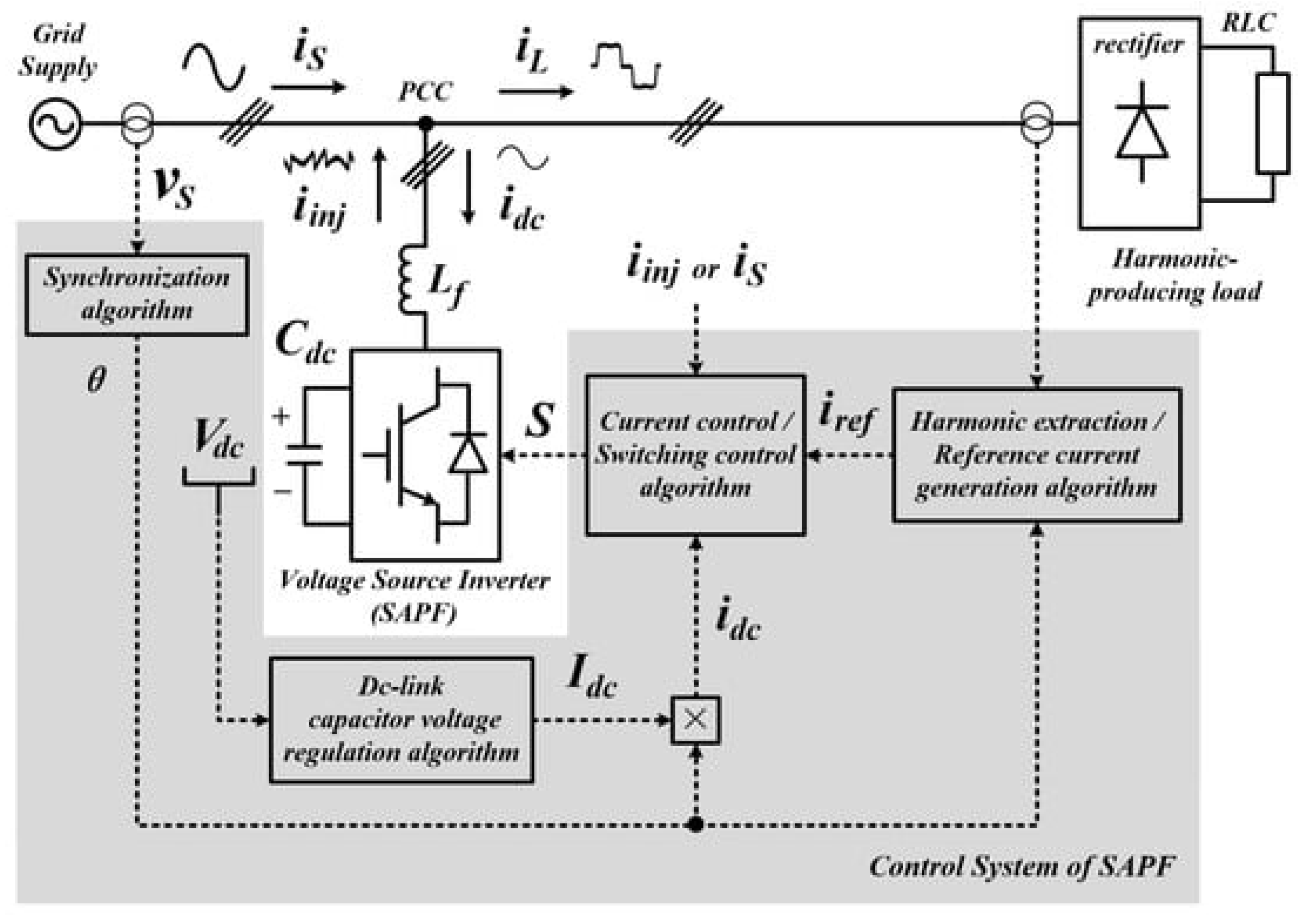
- AI engineering models and meta-heuristic algorithm models are applied to SAPF to perform the extraction of the harmonic component from the measurement signals of the sensors and, at the same time, perform the selection of the optimal compensating current value providing compensation to the power supply;
- Models that combine meta-heuristic algorithm techniques with AI engineering models in shunt adaptive power filter to increase convergence speed into selecting current compensation and improve the quality of the sine wave shape of the power signal.
- The equation relationship between the meta-heuristic algorithm models is also compared via the pseudo-code algorithm;
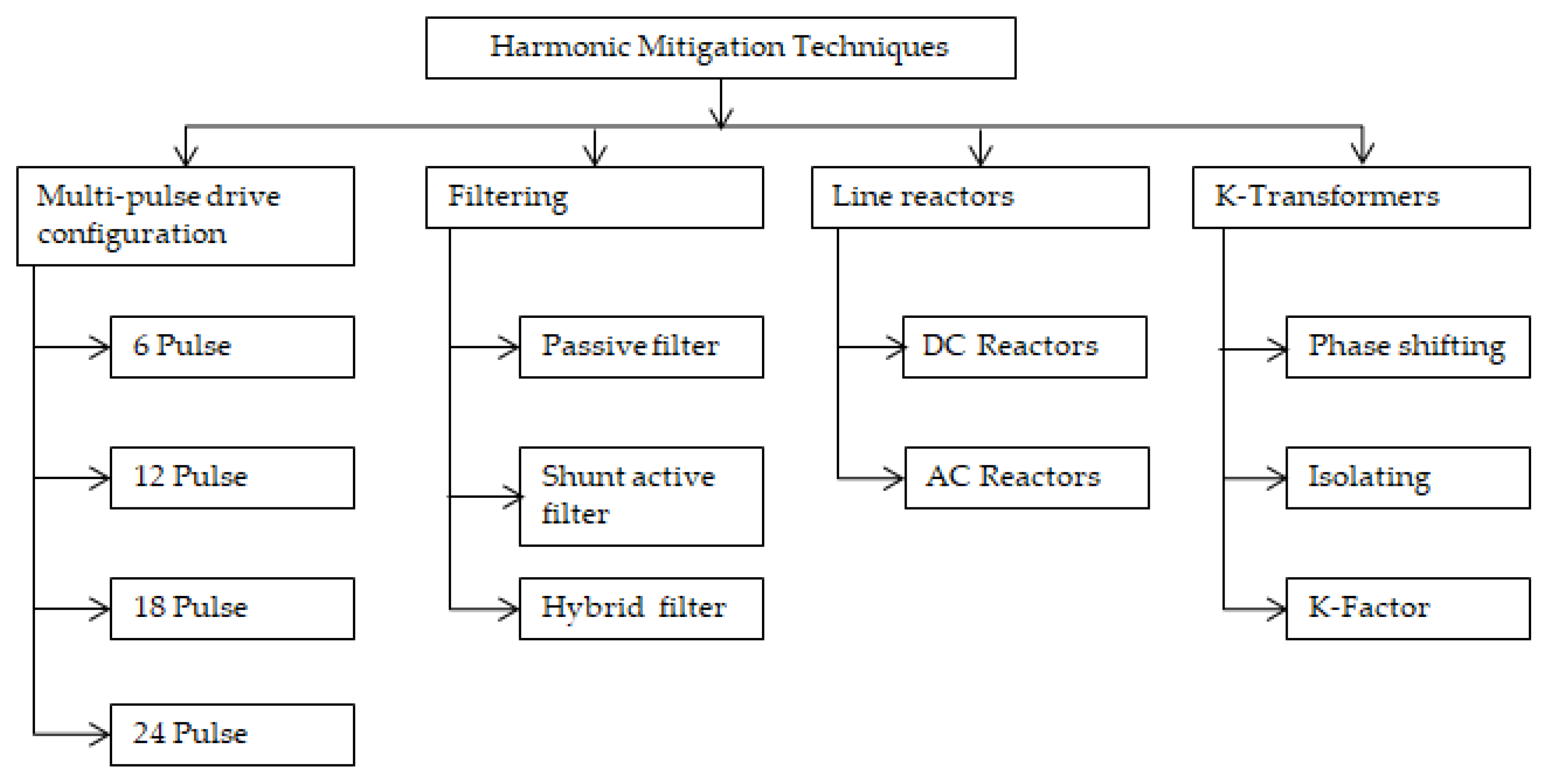
- Overview of applying shunt adaptive power filter to compensate for power loss for power sources that have been connected to the national power grid such as PV Solar, wind power, and combined AI techniques models with meta-heuristic algorithm models into the above power system;
- Overview of current control circuits that compensate for power loss caused by harmonics and harmonic analysis circuits generated in power systems are also described in general.
2. Random Models and Optimization Models
- Meta-heuristic optimization is applied by many researchers to research many aspects of optimization and is widely used, which means that there are many recent research publications in many prestigious journals around the world catalog ISI/SCOPUS and is used in almost every field from engineering to economics and other sciences;
- Artificial intelligence uses meta-heuristic optimization models in training activities and as well as improves the ability to predict results of artificial intelligence (AI) technical models such as artificial neural network (ANN), fuzzy logic, and adaptive neural fuzzy system (ANFIS);
- Meta-heuristic optimization is done very simply with not too complicated mathematical models, with no need for additional training data or initial implementation solutions, just building suitable mathematical models and precise distribution functions’ respective performance to improve the optimization level for the operations;
- Researchers only need to use the population size and number of iterations to build an optimal research model using meta-heuristic optimization without the need to delve into the knowledge of complex mathematical models;
- Researchers only need to build fitness functions and constraints to freely choose meta-heuristic models and modify them to perform optimal problem-solving;
- Meta-heuristic research models are integrated into the test models and validated based on simulation models with various tools available;
- Meta-heuristic optimization gives good processing results for multi-objective processing models and, with many decision variables and constraints, does not restrict solutions and is not dominated;
- Meta-heuristic optimization is used to solve multi-disciplinary problems, and along with many publications in prestigious journals in the world at the present time, it is useful for analysis, comparison, and analysis activities to compare the research results of the proposed work of the authors;
- Compared with the training and learning requirements with complex mathematical models of artificial intelligence (AI) techniques, meta-heuristic optimization shows that the computation process is much simpler with the use of algorithms. Math models are much simpler than those applied in AI techniques;
- Nowadays, the development of computer technology needs to use optimization models more and more to optimize the processing time of real-time problems.
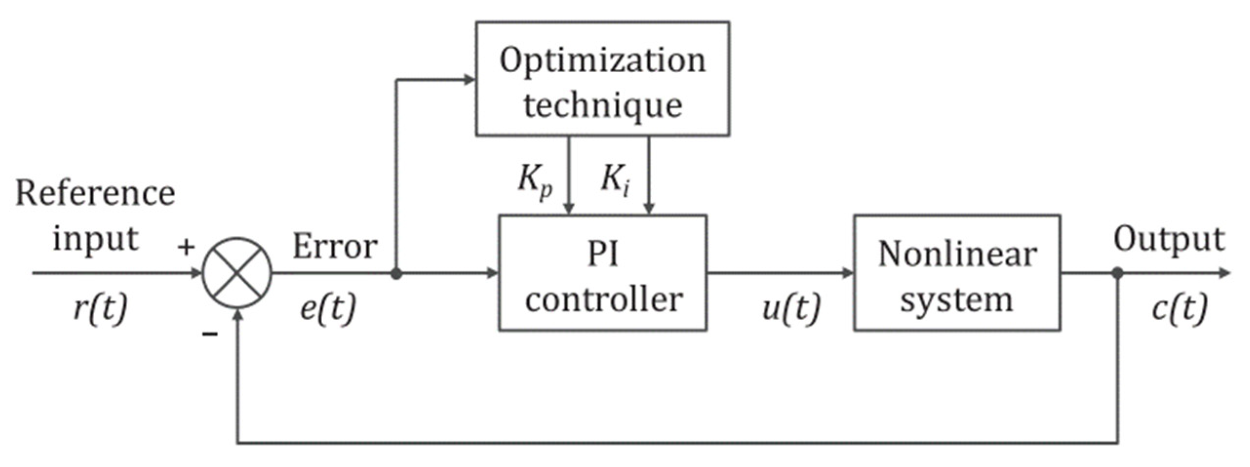
3. Harmonic Mitigation Using Meta-Heuristic Algorithms and Artificial Intelligence
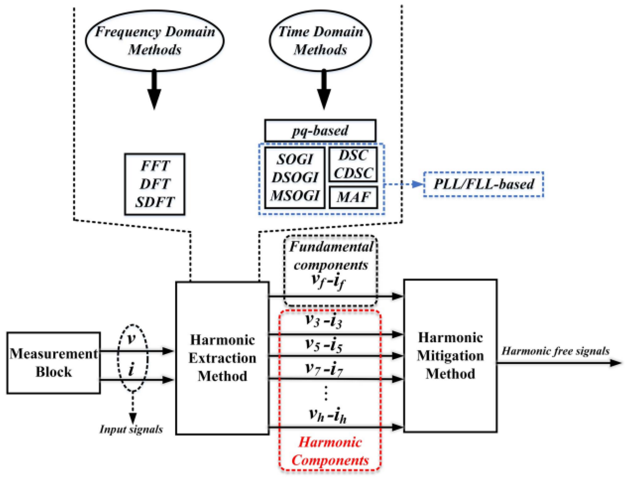
3.1. Analyze and Detect Harmonic Components
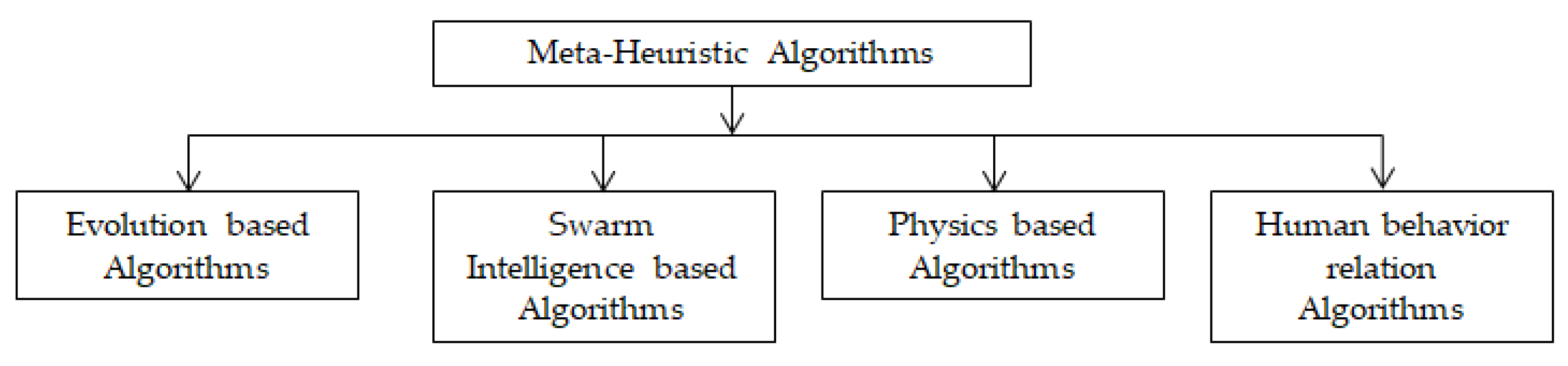
3.2. Harmonic Mitigation Using Meta-Heuristic Algorithms
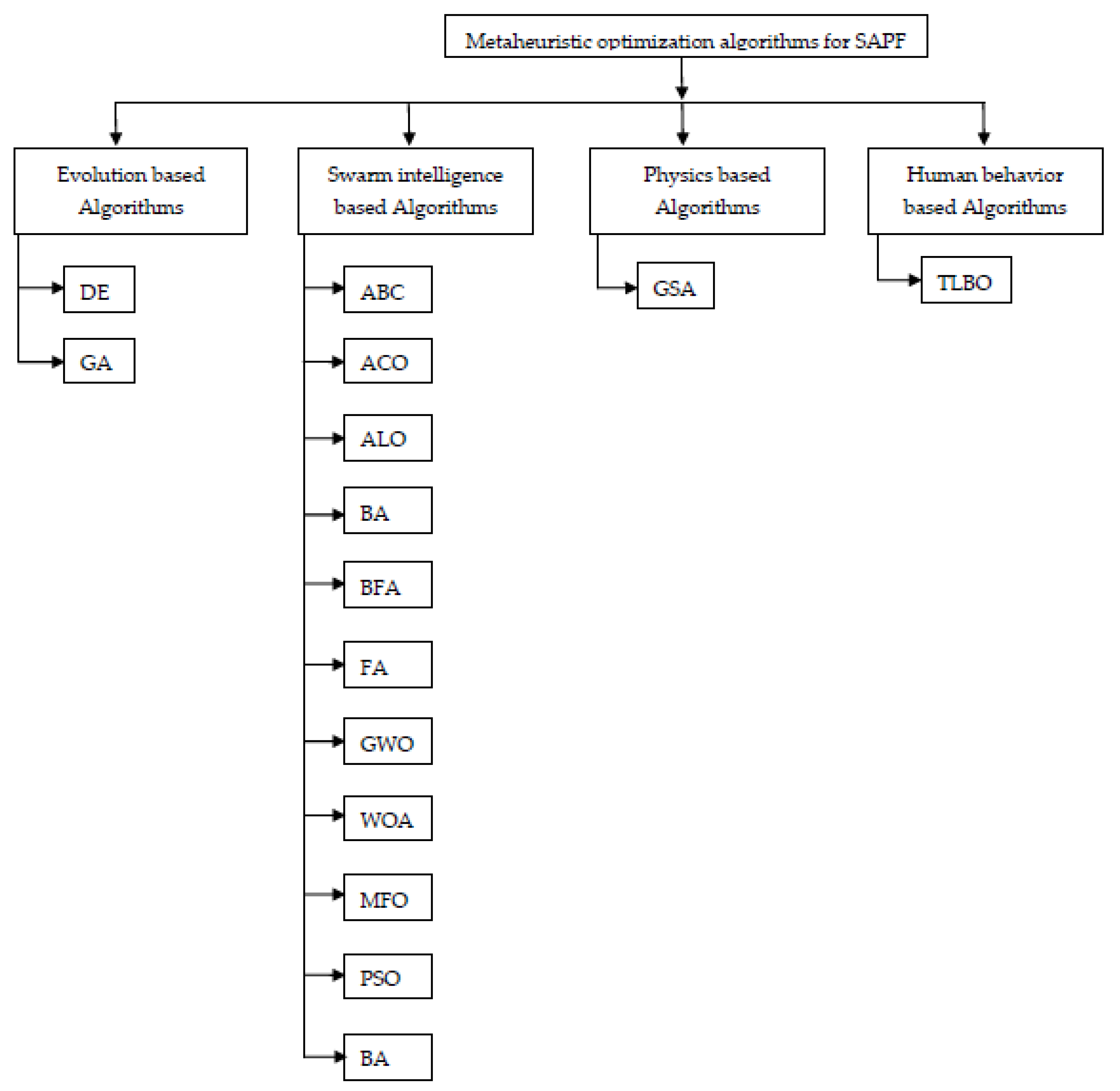
3.2.1. Evolution-Based Algorithms
Difference Evolution Algorithms (DE) for SAPF
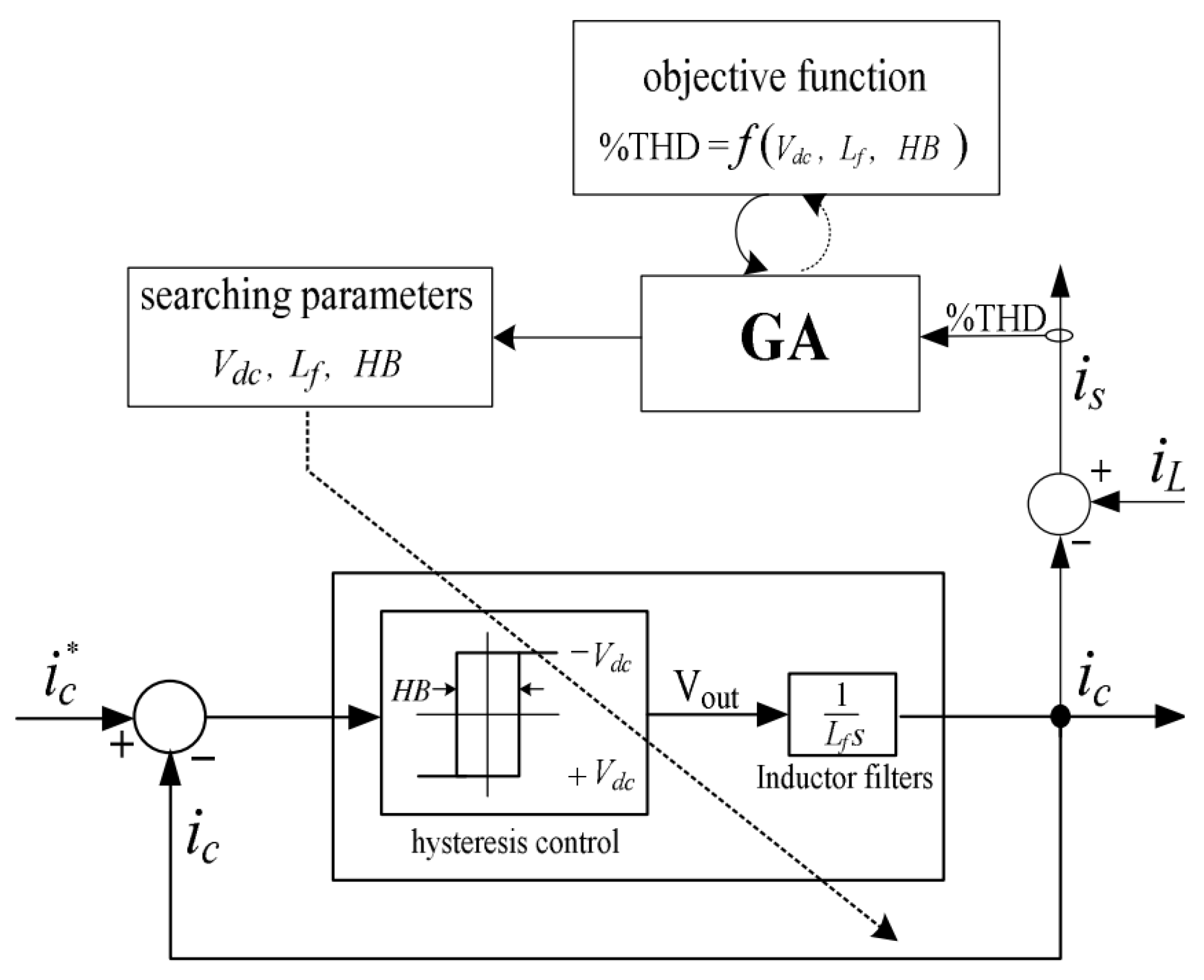
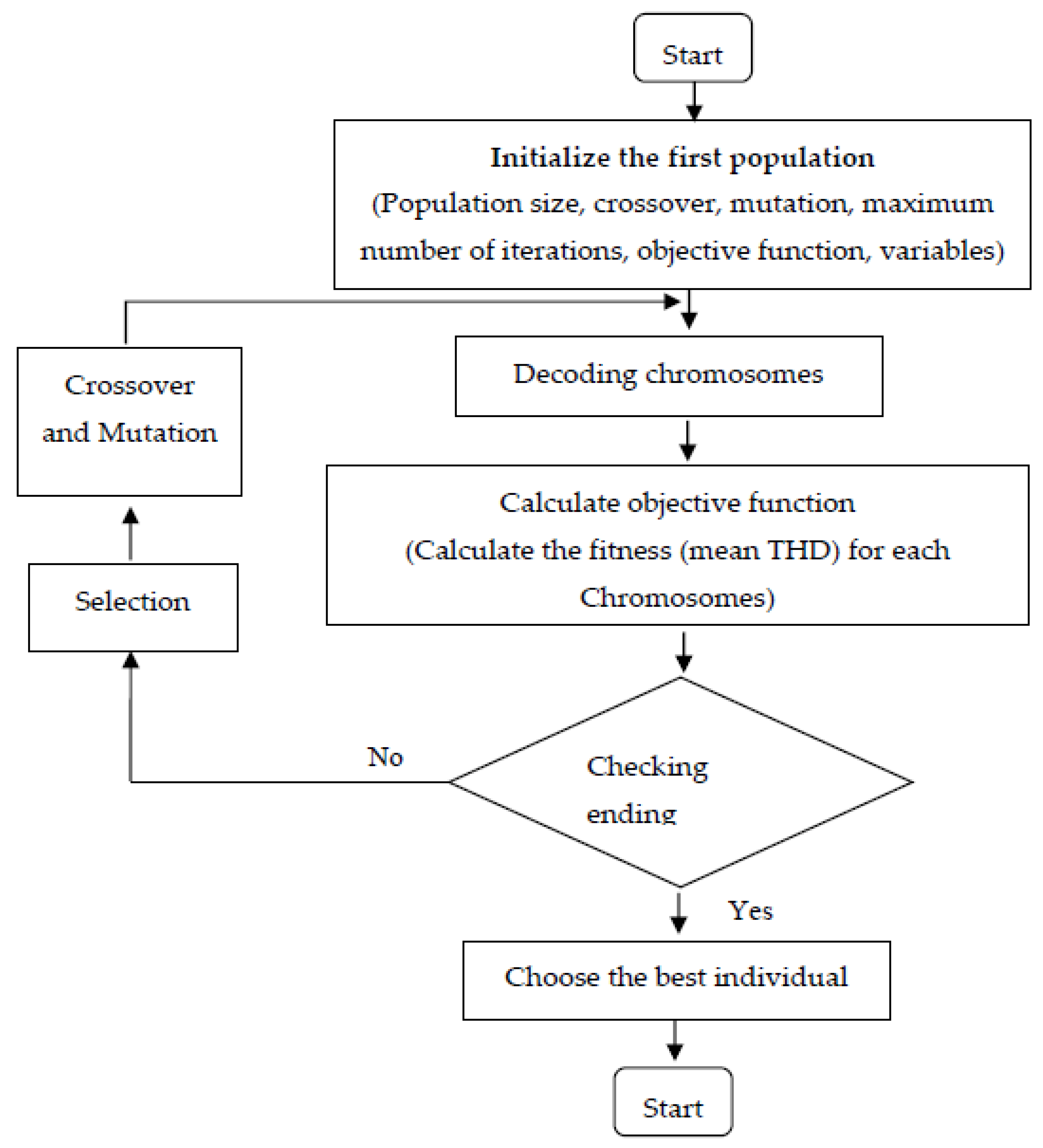
Genetic Algorithms (GAs) Algorithms for SAPF
3.2.2. Swarm Intelligence-Based Algorithms
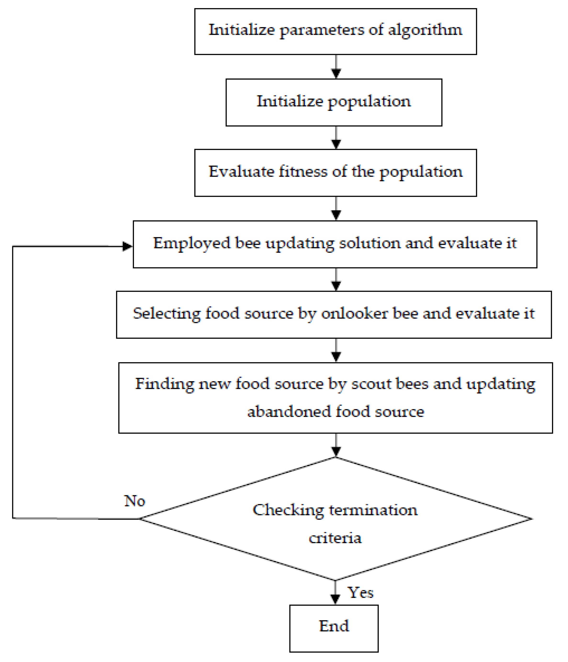
Artificial Bee Colony (ABC) Algorithm for SAPF
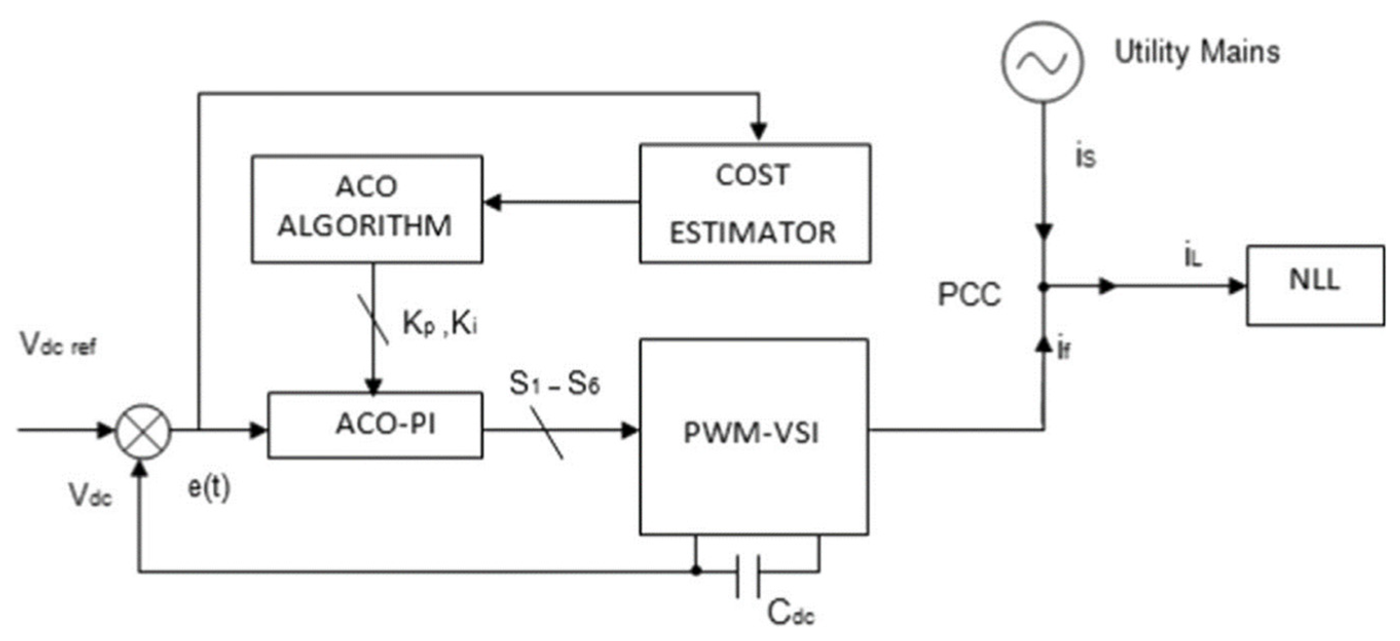
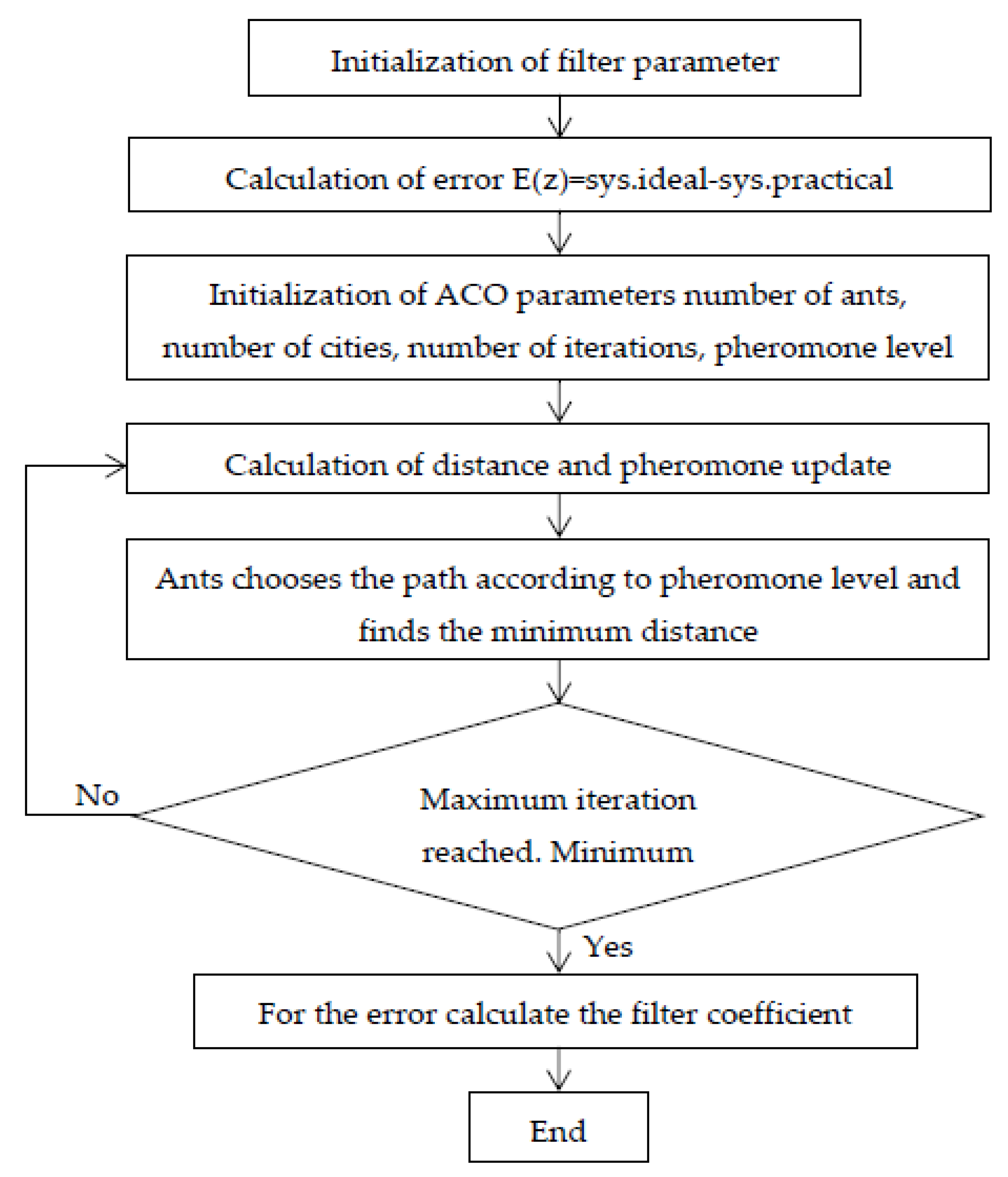
Ant Colony Optimization (ACO) for SAPF
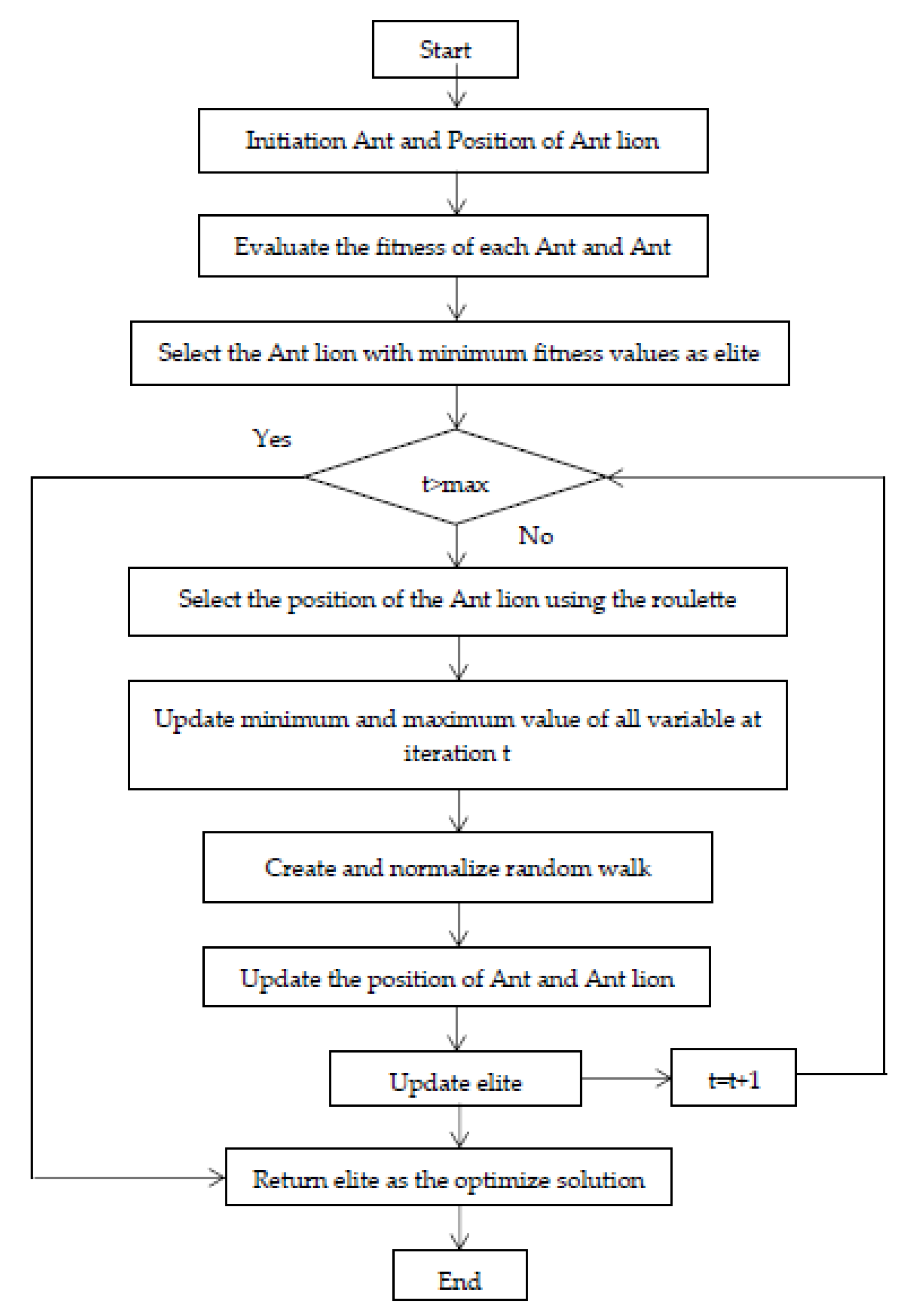
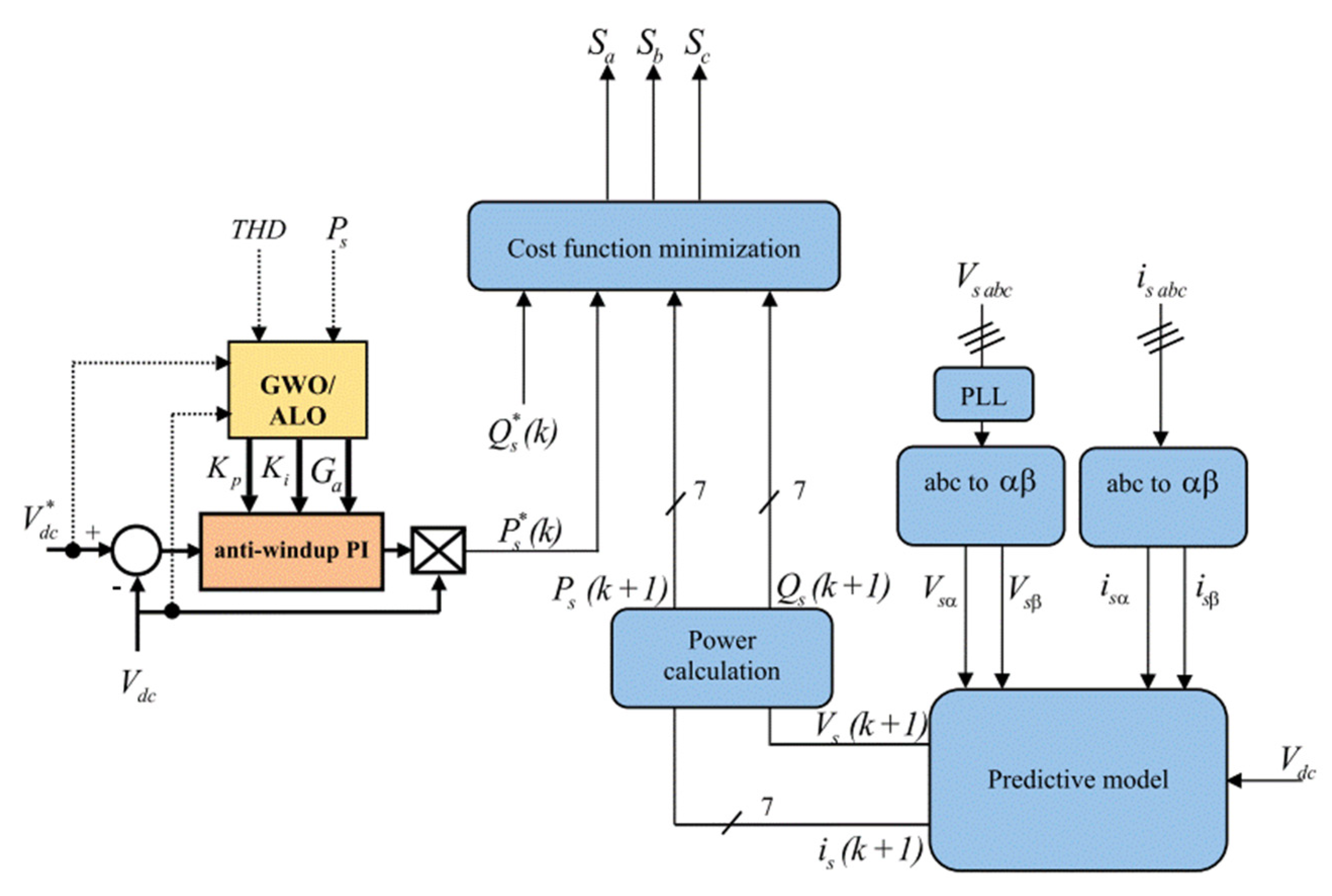
Ant Lion Optimizer (ALO) for SAPF
| Algorithm 1: The pseudo-code of the ALO Algorithm | |||
| 1 | Input (Set input data of SAPF. Set parameters of ALO) | ||
| 2 | K = 1 | ||
| 3 | Create 3 initial sizes of ant and ant lion are | ||
| 4 | Run SAPF with and evaluate the fitness function value of ants and ant lions | ||
| 5 | Identify the best ant lion | ||
| 6 | While do | ||
| 7 | For i = 1 to the number of agents, do: | ||
| 8 | Choose the antlion based on the movement circle | ||
| 9 | Update the position of ants according to Formulas (18) and (19) | ||
| 10 | Update the location of the antlion (update the value) according to Formula (17). | ||
| 11 | Run SAPF updates the value and evaluates the fitness function value of the ant lion | ||
| 12 | Substitute the antlion with ants according to Formula (24) | ||
| 13 | Update elite position | ||
| 14 | K = K + 1 | ||
| 15 | End for | ||
| 16 | End while | ||
| 17 | Return optimization elite | ||
| 18 | Output: Print optimization gains of the PI controller in SAPF according to the optimal elite value | ||
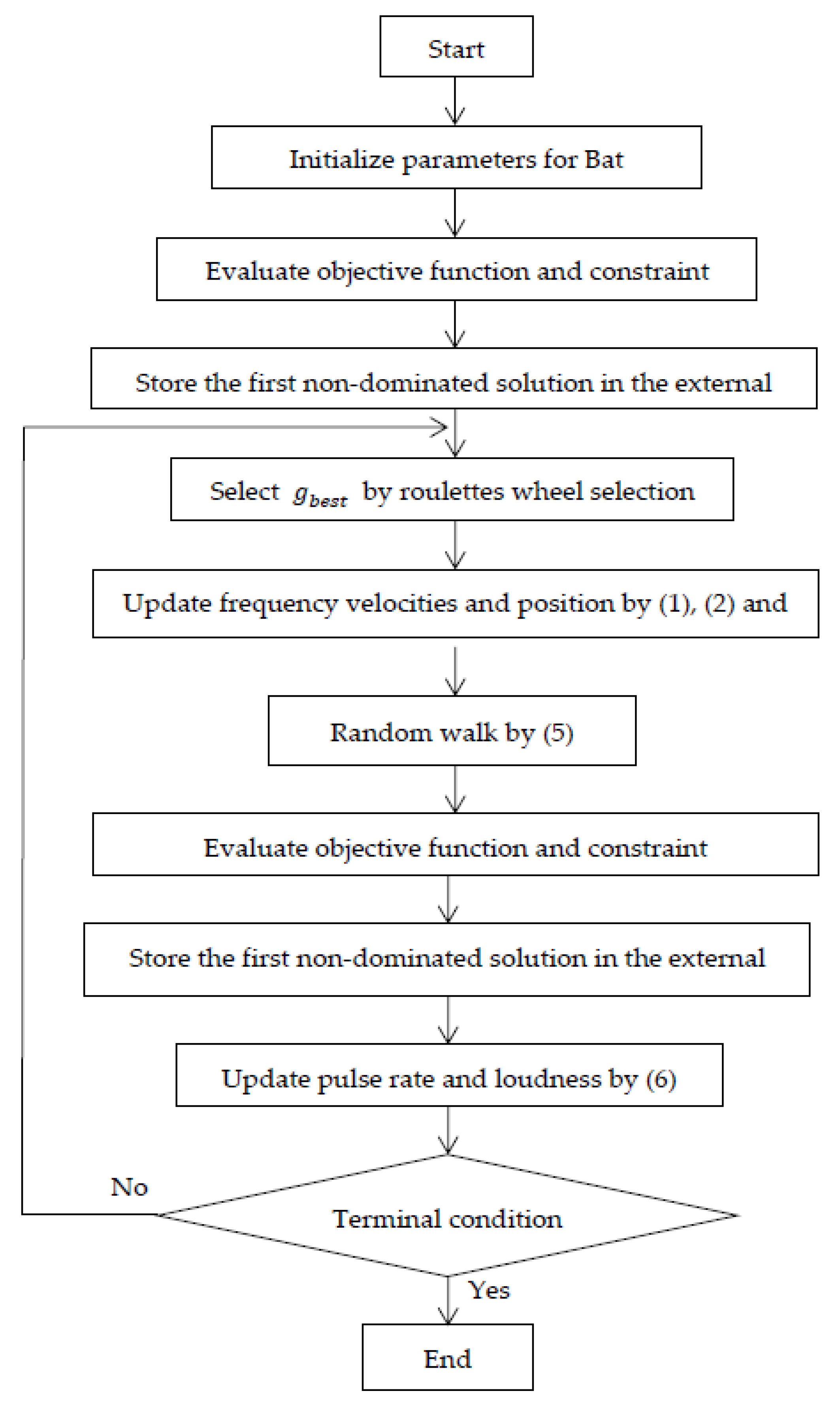
Bat Algorithm (BA) for SAPF
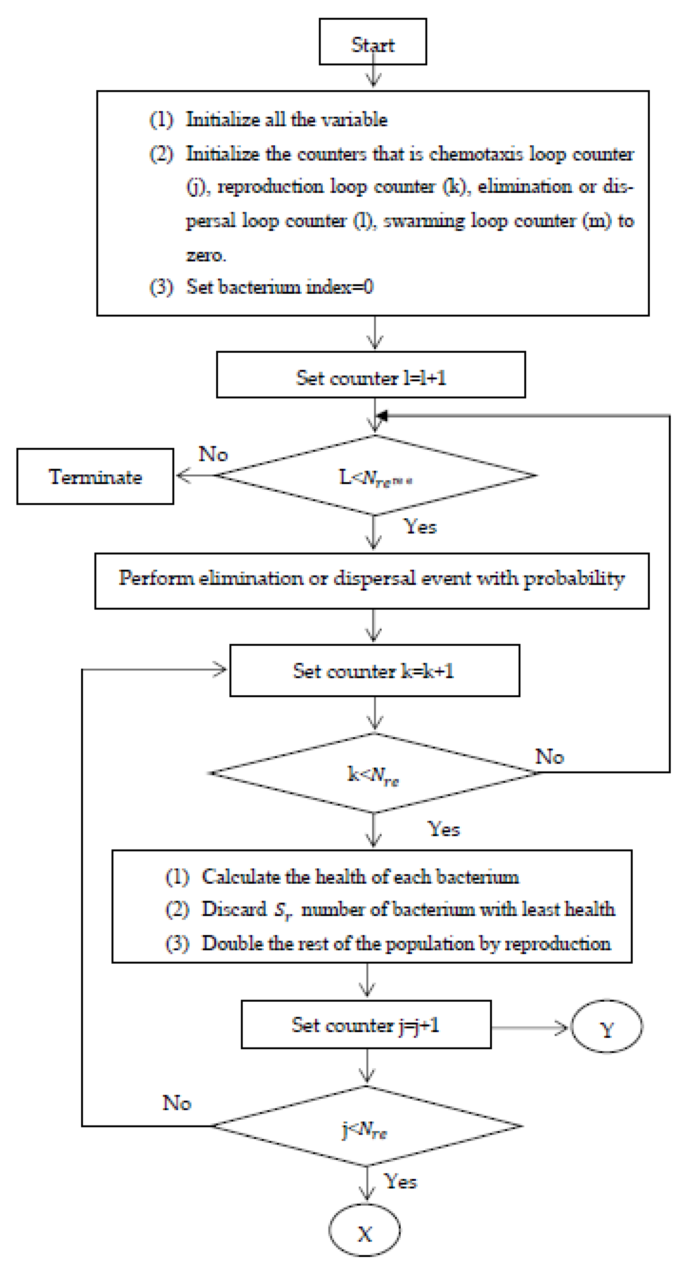
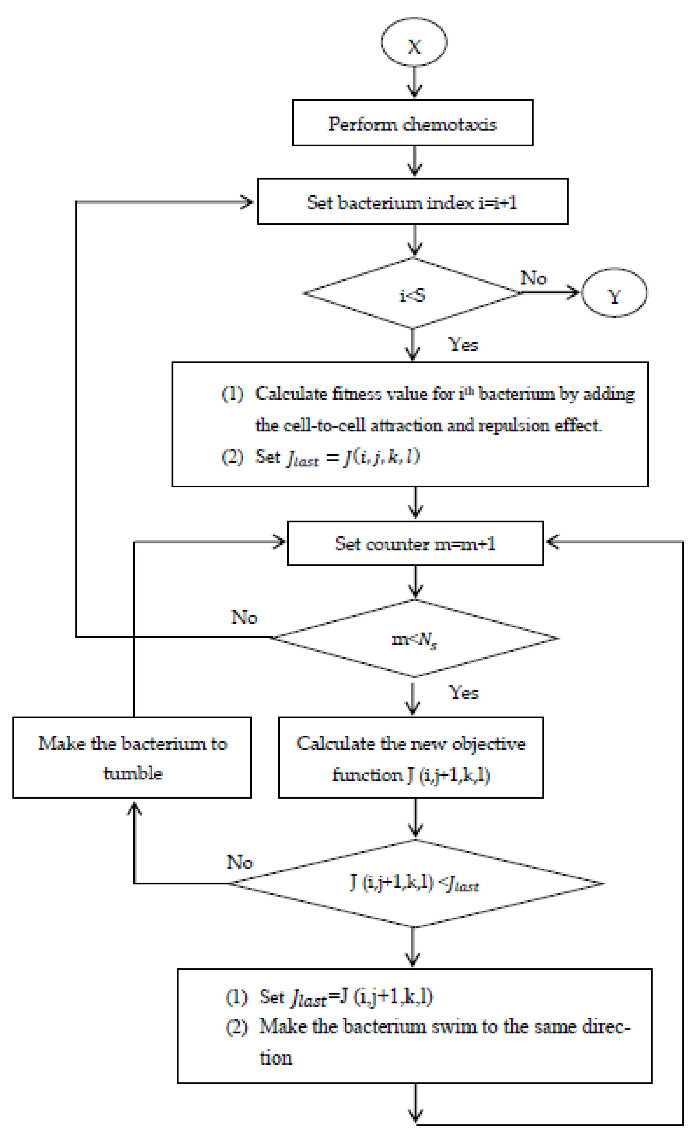
Bacterial Foraging Algorithm (BFA) for SAPF
Firefly Algorithm (FA) for SAPF
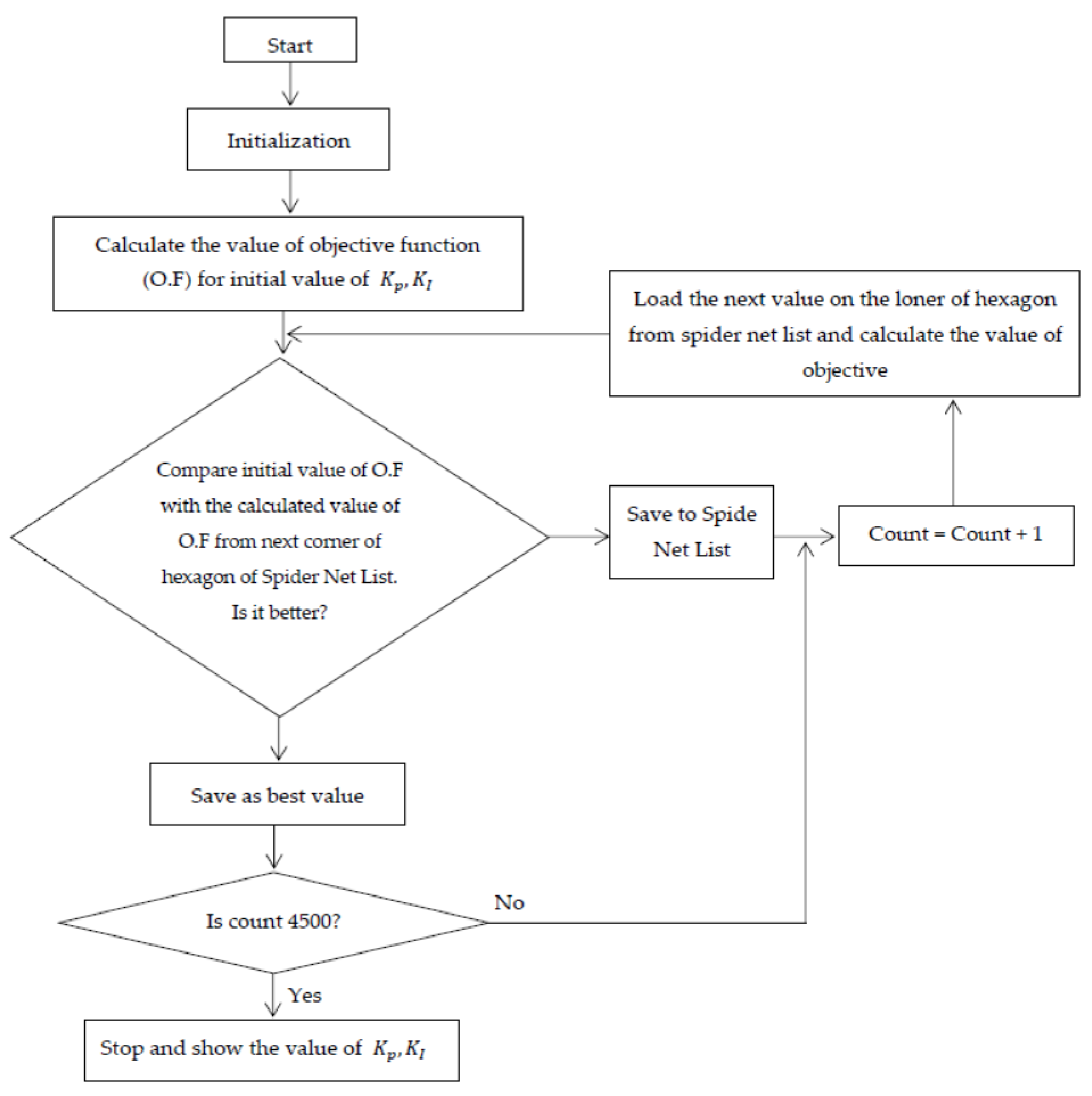
3.2.3. Spider Net Search (ASNS) for SAPF
Adaptive Tabu Search (ATS) for SAPF
Whale Optimization Algorithm (WOA) for SAPF
Swarm Particle Swarm Optimization (PSO) for SAPF
Flower Pollination Algorithm (FPA)
Grey Wolf Optimization (GWO) Algorithm for SAPF
| Algorithm 2: Pseudocode of GWO Algorithms | |||
| 1 | Input (Set input data of SAPF. Set initialize parameters of GWO) | ||
| 2 | K = 1 | ||
| 3 | Create an initial population of search agent with 3 dimension | ||
| 4 | Run SAPF using and evaluate the fitness function value in the search area | ||
| 5 | Sort the positions in the order of first-, second-, and third-best in the search area. | ||
| 6 | While do | ||
| 7 | For i = 1 to the number of search agents, do | ||
| 8 | Update the position and update the value of following Equation (84) | ||
| 9 | Update | ||
| 10 | Update | ||
| 11 | Run SAPF using updated values of and evaluate the fitness function value of the search area. | ||
| 12 | Update | ||
| 13 | K = K + 1 | ||
| 14 | End for | ||
| 15 | End while | ||
| 16 | Return (best solution) | ||
| 17 | Output: Print the optimum again of the PI controller in SAPF in terms of | ||
3.2.4. Physics-Based Algorithms
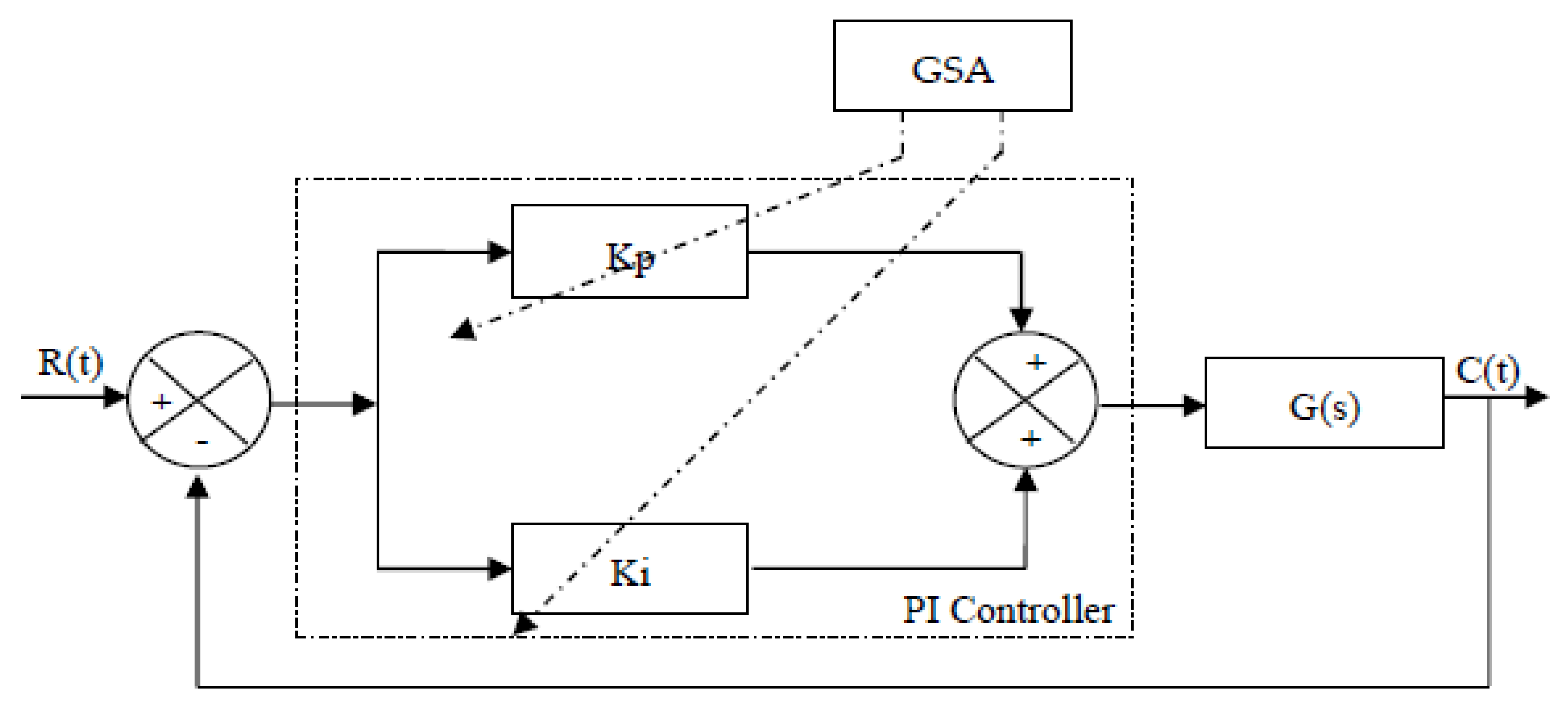
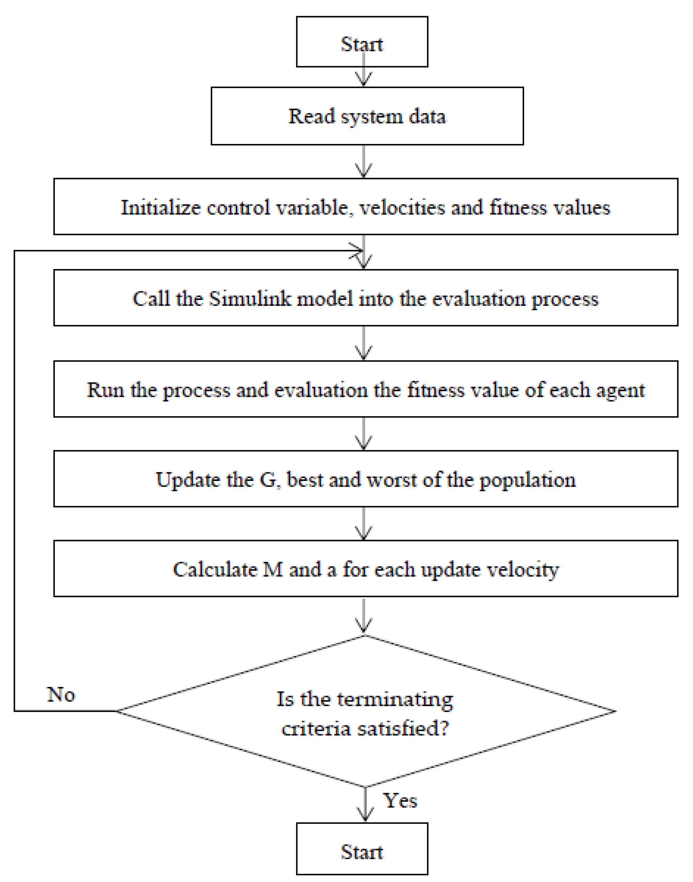
Gravitational Search Algorithm (GSA) for SAPF
3.2.5. Human Behavior Relation Algorithms
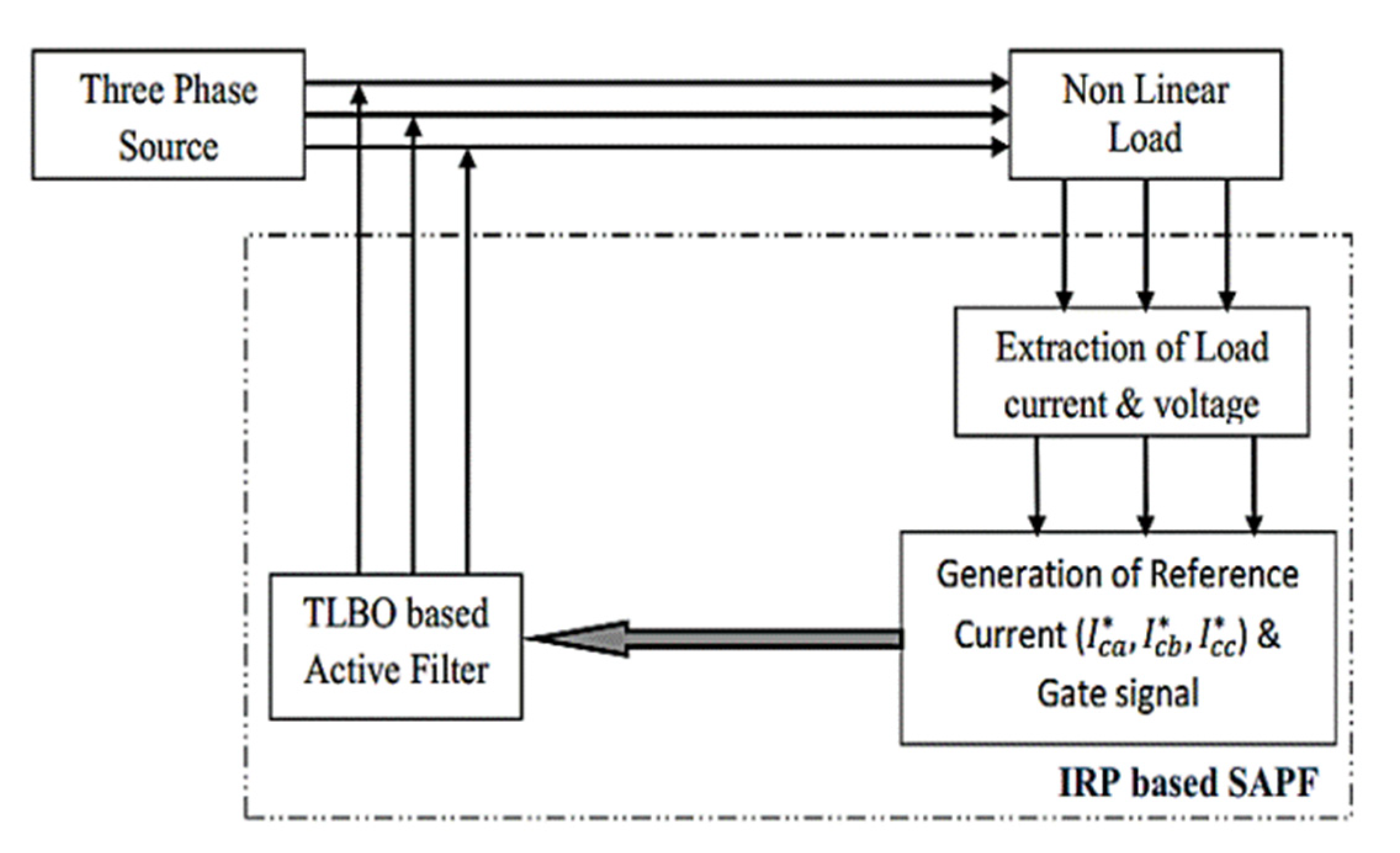
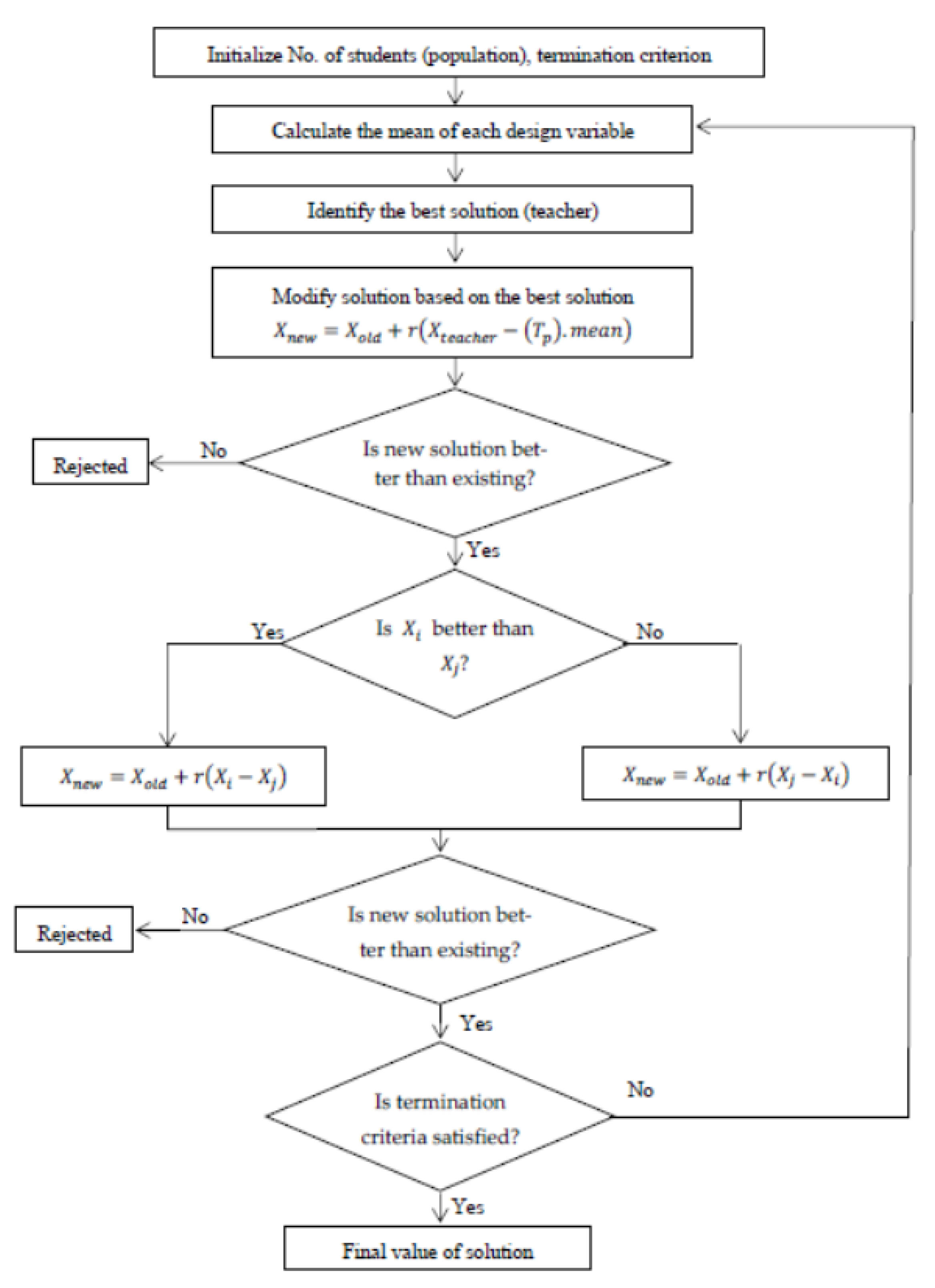
Teaching-Learning-Based Optimization (TLBO)
4. Discussion and Future Research Problems
- Implement improvements to some modern meta-heuristic optimization algorithms to improve functionality and improve optimal performance. In particular, PSO has a fast convergence speed but is limited in the search area, and there is a risk of virtual convergence; it is necessary to have a method to solve the search area which ensures the provision of a complete and accurate hammock number to respond to the best converged PSO optimization algorithm. For example, hybrid optimization methods include GA-PSO and DE-PSO;
- Development of hybrid optimization algorithms between modern meta-heuristic optimization algorithms to solve each other’s weaknesses and enhance each other’s strengths;
- Further changes and improvements are needed to the local and global models of some meta-heuristic optimization algorithms as the trade-off changes the complexity level between them;
- The operation of fine-tuning the parameters of meta-heuristic optimization algorithms in solving optimization problems to be solved thoroughly in order to improve the optimal efficiency;
- Some meta-heuristic optimization algorithms need to develop more parameters to improve the accuracy of convergence results;
- Evaluating the performance of meta-heuristic optimization algorithms by statistical models needs to be developed;
- Solving big data-related content problems with meta-heuristic optimization algorithms needs to use transformation learning to enhance its optimal performance;
- A population parameter is the cause of delay in optimal processing time in optimization problem solving of modern meta-heuristic optimization algorithms;
- The parameters of meta-heuristic optimization algorithms, including exploration, mining, searchability, convergence, and local convergence, need to be proven by specific theoretical models and mathematical models;
- The strong growth of IOT devices used in the industrial 4.0 environment creates big data problems with their complexity and imbalance. Many numbers of decision-making variables are formed. The self-expanding meta-heuristic optimization algorithms feature self-adjusting and evolving to respond to solving big data problems;
- There is a need for a specific way to identify subsets or classes of problems that meet the criteria for selecting the optimal meta-heuristic algorithm that meets the best convergence performance.
5. Conclusions
Author Contributions
Funding
Data Availability Statement
Acknowledgments
Conflicts of Interest
References
- Li, D.; Wang, T.; Pan, W.; Ding, X.; Gong, J. A comprehensive review of improving power quality using active power filters. Electr. Power Syst. Res. 2021, 199, 107389. [Google Scholar] [CrossRef]
- Soliman, H.M.; Saleem, A.; Bayoumi, E.H.E.; De Santis, M. Harmonic Distortion Reduction of Transformer-Less Grid-Connected Converters by Ellipsoidal-Based Robust Control. Energies 2023, 16, 1362. [Google Scholar] [CrossRef]
- Adineh, B.; Keypour, R.; Davari, P.; Blaabjerg, F. Review of Harmonic Mitigation Methods in Microgrid: From a Hierarchical Control Perspective. IEEE J. Emerg. Sel. Top. Power Electron. 2020, 9, 3044–3060. [Google Scholar] [CrossRef]
- Aziz, M.H.A.; Azizan, M.M.; Sauli, Z.; Yahya, M.W. A review on harmonic mitigation method for non-linear load in electrical power system. Proceeding Green Des. Manuf. 2020, 2239, 020022. [Google Scholar] [CrossRef]
- Keypour, R.; Adineh, B.; Khooban, M.H.; Blaabjerg, F. A New Population-Based Optimization Method for online Minimization of Voltage Harmonics in Islanded Microgrids. IEEE Trans. Circuits Syst. II Express Briefs 2019, 67, 1084–1088. [Google Scholar] [CrossRef]
- Langlang, G.; Arif, N.A.; Denis, E.C.; Eli, H.S.; Ahmad, A.B.A. Application of line reactors and harmonic filter in electric power system are integrated renewable energy in Mesh topology. In Proceedings of the 2022 4th International Conference on Cybernetics and Intelligent System (ICORIS) IEEE, Prapat, Indonesia, 8–9 October 2022; pp. 1–5. [Google Scholar] [CrossRef]
- Manish, V.; Neeraj, B.; Scott, D.; Todd, O. Isolation Techniques for Medium-Voltage Adjustable Speed Drives. IEEE Ind. Appl. Mag. 2019, 1, 1077–2018. [Google Scholar] [CrossRef]
- Zailan, F.H.; Soomro, D.M. Mitigating Harmonics by using K-transformer. Evol. Electr. Electron. Eng. 2022, 3, 510–515. [Google Scholar]
- Abbas, A.S.; El-Sehiemy, R.A.; Abou El-Ela, A.; Ali, E.S.; Mahmoud, K.; Lehtonen, M.; Darwish, M.M.F. Optimal Harmonic Mitigation in Distribution Systems with Inverter Based Distributed Generation. Appl. Sci. 2021, 11, 774. [Google Scholar] [CrossRef]
- Iturra, R.G.; Cruse, M.; Figge, K.; Thiemann, P.; Dresel, C. Ultra-Low Losses SiC-Based Active Damper for Industrial Power Systems: Mitigating Harmonic Distortion and Maximizing Harmonic Power Recovery. IEEE Trans. Energy Convers. 2022, 37, 2926–2940. [Google Scholar] [CrossRef]
- Park, B.; Lee, J.; Yoo, H.; Jang, G. Harmonic Mitigation Using Passive Harmonic Filters: Case Study in a Steel Mill Power System. Energies 2021, 14, 2278. [Google Scholar] [CrossRef]
- Chuen, L.T.; Chee, W.T. DC traction power substation using an eighteen-pulse rectifier transformer system. Int. J. Power Electron. Drive Syst. 2021, 12, 2284–2394. [Google Scholar] [CrossRef]
- Du, Q.; Fang, Z.; Gao, L.; Li, Q.; Li, F.; Meng, F. Open-Phase Fault Research on the Parallel-Connected 40-Pulse Rectifier with Multi-Output Auto-Connected Phase-Shifting Transformer. IEEE J. Emerg. Sel. Top. Power Electron. 2023, 1, 1–8. [Google Scholar] [CrossRef]
- Ghayal, S.P.; Gour, S. Analysis of harmonics and neutral to ground (N to G) voltage diminution nusing isolation transformer. In Proceedings of the 2017 Third International Conference on Science Technology Engineering & Management (ICONSTEM), Chennai, India, 23–24 March 2017; Volume 17, pp. 1–4. [Google Scholar] [CrossRef]
- Ragonese, E.; Spina, N.; Parisi, A.; Palmisano, G. An Experimental Comparison of Galvanically Isolated DC-DC Converters: Isolation Technology and Integration Approach. Electronics 2021, 10, 1186. [Google Scholar] [CrossRef]
- Yu, Q.; Chu, S.; Li, W.; Tian, L.; Wang, X.; Cheng, Y. Electromagnetic Shielding Analysis of a Canned Permanent Magnet Motor. IEEE Trans. Ind. Electron. 2019, 67, 8123–8130. [Google Scholar] [CrossRef]
- Lu, G.; Zheng, D.; Zhang, Q.; Zhang, P. Effects of Converter Harmonic Voltages on Transformer Insulation Ageing and an Online Monitoring Method for Interlayer Insulation. IEEE Trans. Power Electron. 2022, 37, 3504–3514. [Google Scholar] [CrossRef]
- Hoon, Y.; Mohd Radzi, M.A.; Mohd Zainuri, M.A.A.; Zawawi, M.A.M. Shunt Active Power Filter: A Review on Phase Synchronization Control Techniques. Electronics 2019, 8, 791. [Google Scholar] [CrossRef]
- Sanjan, P.S.; Gowtham, N.; Bhaskar, M.S.; Subramaniam, U.; Almakhles, D.J.; Padmanaban, S.; Yamini, N.G. Enhancement of Power Quality in Domestic Loads Using Harmonic Filters. IEEE Access 2020, 8, 197730–197744. [Google Scholar] [CrossRef]
- Thulaseedharan, K.R.; Parambil, A.; Puthenveetil, M.J.; Arunodayam, R.A. Compact microstrip plowpass filter with high harmonics suppression using defected structures. AEU Int. J. Electron. Commun. 2020, 115, 153032. [Google Scholar] [CrossRef]
- Du, Q.; Gao, L.; Li, Q.; Liu, W.; Yin, X.; Meng, F. Harmonic Reduction Methods at DC Link of Series-Connected Multi-Pulse Rectifiers: A Review. IEEE Trans. Power Electron. 2022, 37, 3143–3160. [Google Scholar] [CrossRef]
- Kim, J.; Lai, J.-S. Analysis of a Shunt Wye-Delta Transformer for Multi-Generator Harmonic Elimination Under Non-Ideal Phase-Shift Conditions. IEEE Trans. Ind. Appl. 2019, 55, 2412–2420. [Google Scholar] [CrossRef]
- Cheng, Q.; Wang, C.; Wang, J. Analysis on Displacement Angle of Phase-Shifted Carrier PWM for Modular Multilevel Converter. Energies 2020, 13, 6743. [Google Scholar] [CrossRef]
- Stephen, B.J.; Emmanuel, G.D.; Afeez, A.; David, O.O.; Ban, M.K. Metaheuristic algorithms for PID controller parameters tuning: Review, approaches and open problems. Helyon 2022, 8, e09399. [Google Scholar] [CrossRef]
- Yang, B.; Wang, J.; Zhang, X.; Yu, T.; Yao, W.; Shu, H.; Sun, L. Comprehensive overview of meta-heuristic algorithm applications on PV cell parameter identification. Energy Convers. Manag. 2020, 208, 112595. [Google Scholar] [CrossRef]
- IEEE Std 519™-2022; IEEE Standard for Harmonic Control in Electric Power Systems. Transmission and Distribution Committee of the IEEE Power and Energy Society. The Institute of Electrical and Electronics Engineers, Inc. 3 Park Avenue: New York, NY, USA, 2022; STDPD25432. pp. 10016–15997. [CrossRef]
- Jaros, R.; Byrtus, R.; Dohnal, J.; Danys, L.; Baros, J.; Koziorek, J.; Zmij, P.; Martinek, R. Advanced Signal Processing Methods for Condition Monitoring. Arch. Computat. Methods Eng. 2022, 1163, 1553–1577. [Google Scholar] [CrossRef]
- Hanna, N.A.F.; Fadel, M.; Kanaan, H.Y. Design of a direct control strategy for a static shunt compensator to improve power quality in polluted and unbalanced grids. Math. Comput. Simul. 2018, 158, 199–215. [Google Scholar] [CrossRef]
- Ouchen, S.; Gaubert, J.-P.; Steinhart, H.; Betka, A. Energy quality improvement of three-phase shunt active power filter under different voltage conditions based on predictive direct power control with disturbance rejection principle. Math. Comput. Simul. 2018, 158, 506–519. [Google Scholar] [CrossRef]
- Gao, T.; Lin, Y.; Chen, D.; Xiao, L. A novel active damping control based on grid-side current feedback for LCL-filter active power filter. Energy Rep. 2020, 6, 1318–1324. [Google Scholar] [CrossRef]
- Xiao, G.; Hongyi, L.; Guozhu, C. SiC-MOSFET shunt active power filter based on half-cycle SDFT and repetitive control. Energy Rep. 2021, 7, 246–252. [Google Scholar] [CrossRef]
- Karthikeyan, M.; Sharmilee, K.; Balasubramaniam, P.M.; Prakash, N.B.; Rajesh Babu, M.; Subramaniyaswamy, V.; Sudhakar, S. Design and Implementation of ANN-based SAPF Approach for Current Harmonics Mitigation in Industrial Power Systems. Microprocess. Microsyst. 2020, 77, 103194. [Google Scholar] [CrossRef]
- Agrawal, S.; Palwalia, D.K.; Kumar, M. Performance Analysis of ANN Based three-phase four-wire Shunt Active Power Filter for Harmonic Mitigation under Distorted Supply Voltage Conditions. IETE J. Res. 2019, 68, 566–574. [Google Scholar] [CrossRef]
- Chen, D.; Xiao, L.; Lian, H.; Xu, Z. A fault tolerance method based on switch redundancy for shunt active power filter. Energy Rep. 2021, 7, 449–457. [Google Scholar] [CrossRef]
- Chen, D.; Xiao, L.; Yan, W.; Li, Y.; Guo, Y. A harmonics detection method based on triangle orthogonal principle for shunt active power filter. Energy Rep. 2021, 7, 98–104. [Google Scholar] [CrossRef]
- Dongdong, C.; Long, X.; Wenduan, Y.; Yan, L.; Yinbiao, G. A heat dissipation design strategy based on computational fluid dynamics analysis method for shunt active power filter. Energy Rep. 2022, 8, 229–238. [Google Scholar] [CrossRef]
- Amit, V. Shunt active power filtering with reference current generation based on dual second order generalized integrator and LMS algorithm. Energy Rep. 2022, 8, 886–893. [Google Scholar] [CrossRef]
- Hiral, H.; Vaidehi, D.; Amit, V. Modified symmetrical sinusoidal integrator and instantaneous reactive power theory-based control of shunt active filter. Energy Rep. 2022, 8, 515–523. [Google Scholar] [CrossRef]
- Fang, Y.; Fei, J.; Wang, T. Adaptive Backstepping Fuzzy Neural Controller Based on Fuzzy Sliding Mode of Active Power Filter. IEEE Access 2020, 8, 96027–96035. [Google Scholar] [CrossRef]
- Liu, L.; Fei, J.; An, C. Adaptive Sliding Mode Long Short-Term Memory Fuzzy Neural Control for Harmonic Suppression. IEEE Access 2021, 9, 69724–69734. [Google Scholar] [CrossRef]
- Radhamani, R.; Balamurugan, R. An Enhanced Modified Multiport Interleaved Flyback Converter for Photovoltaic-Shunt Active Power Filter (PV-SHAPF) Applications. Int. Trans. Electr. Energy Syst. 2022, 2022, 1537319. [Google Scholar] [CrossRef]
- Martinek, R.; Rzidky, J.; Jaros, R.; Bilik, P.; Ladrova, M. Least Mean Squares and Recursive Least Squares Algorithms for Total Harmonic Distortion Reduction Using Shunt Active Power Filter Control. Energies 2019, 12, 1545. [Google Scholar] [CrossRef]
- Baros, J.; Sotola, V.; Bilik, P.; Martinek, R.; Jaros, R.; Danys, L.; Simonik, P. Review of Fundamental Active Current Extraction Techniques for SAPF. Sensors 2022, 22, 7985. [Google Scholar] [CrossRef]
- Martinek, R.; Bilik, P.; Baros, J.; Brablik, J.; Kahankova, R.; Jaros, R.; Danys, L.; Rzidky, J.; Wen, H. Design of a Measuring System for Electricity Quality Monitoring within the SMART Street Lighting Test Polygon: Pilot Study on Adaptive Current Control Strategy for Three-Phase Shunt Active Power Filters. Sensors 2020, 20, 1718. [Google Scholar] [CrossRef] [PubMed]
- Bilal, P.M.; Zaheer, H.; Garcia-Hernandez, L.; Abraham, A. Differential Evolution: A review of more than two decades of research. Eng. Appl. Artif. Intell. 2020, 90, 103479. [Google Scholar] [CrossRef]
- Jesús, G.F.; Carlos, A. Indicator-based Multi-objective Evolutionary Algorithms: A Comprehensive Survey. ACM Comput. Surv. 2020, 53, 1–35. [Google Scholar] [CrossRef]
- Rostami, M.; Berahmand, K.; Nasiri, E.; Forouzandeh, S. Review of swarm intelligence-based feature selection methods. Eng. Appl. Artif. Intell. 2021, 100, 104210. [Google Scholar] [CrossRef]
- Tang, J.; Liu, G.; Pan, Q. A Review on Representative Swarm Intelligence Algorithms for Solving Optimization Problems: Applications and Trends. IEEE/CAA J. Autom. 2021, 8, 1627–1643. [Google Scholar] [CrossRef]
- Shashank, R.V.; Sai, N.B.; John, C.M.; Elizabeth, M. A review of physics-based machine learning in civil engineering. Results Eng. 2022, 13, 100316. [Google Scholar] [CrossRef]
- Burton, J.W.; Stein, M.; Jensen, T.B. A systematic review of algorithm aversion in augmented decision making. J. Behav. Decis. Mak. 2019, 33, 220–239. [Google Scholar] [CrossRef]
- Lorenz-Spreen, P.; Lewandowsky, S.; Sunstein, C.R.; Hertwig, R. How behavioural sciences can promote truth, autonomy, and democratic discourse online. Nat. Hum. Behav. 2020, 4, 1102–1109. [Google Scholar] [CrossRef]
- Micallef, A. A Review of the Current Challenges and Methods to Mitigate Power Quality Issues in Single-Phase Microgrids. IET Gener. Transm. Distrib. 2018, 13, 2044–2054. [Google Scholar] [CrossRef]
- Khan, I.; Vijay, J.; Doolla, S. Nonlinear Load Harmonic Mitigation Strategies in Microgrids: State of the Art. IEEE Syst. J. 2022, 16, 4243–4255. [Google Scholar] [CrossRef]
- Schweizer, D.; Ried, V.; Rau, G.C.; Tuck, J.E.; Stoica, P. Comparing Methods and Defining Practical Requirements for Extracting Harmonic Tidal Components from Groundwater Level Measurements. Math. Geosci. 2021, 53, 1147–1169. [Google Scholar] [CrossRef]
- Kashif, M.; Hossain, M.J.; Fernandez, E.; Taghizadeh, S.; Sharma, V.; Ali, S.M.N.; Irshad, U.B. A Fast Time-Domain Current Harmonic Extraction Algorithm for Power Quality Improvement Using Three-Phase Active Power Filter. IEEE Access 2020, 8, 103539–103549. [Google Scholar] [CrossRef]
- Chen, D.; Lin, Y.; Xiao, L.; Xu, Z.; Lian, H. A harmonics detection method based on an improved comb filter of sliding discrete Fourier for the grid-tied inverter. Energy Rep. 2020, 6, 1303–1311. [Google Scholar] [CrossRef]
- Imam, A.A.; Sreerama Kumar, R.; Al-Turki, Y.A. Modeling and Simulation of a PI Controlled Shunt Active Power Filter for Power Quality Enhancement Based on P-Q Theory. Electronics 2020, 9, 637. [Google Scholar] [CrossRef]
- Zhen, Y.T.; Yap, H.; Mohd, A.M. Synchronous Reference Frame with Finite Impulse Response Filter for Operation of Single-phase Shunt Active Power Filter. In Proceedings of the MATEC Web Conference 14th EURECA 2020—International Engineering and Computing Research Conference “Shaping the Future through Multidisciplinary Research”, Subang Jaya, Malaysia, 25 November 2020; Volume 335, pp. 1–8. [Google Scholar] [CrossRef]
- Xu, M.; Sang, Z.; Li, X.; You, Y.; Dai, D. An Observer-Based Harmonic Extraction Method with Front SOGI. Machines 2022, 10, 95. [Google Scholar] [CrossRef]
- Chi, Y.; Yang, S.; Jiao, W.; He, J.; Gu, X.; Papatheou, E. Spectral DCS-based feature extraction method for rolling element bearing pseudo-fault in the rotor-bearing system. Measurement 2018, 132, 22–34. [Google Scholar] [CrossRef]
- Kashif, M.; Hossain, M.J.; Nawazish Ali, S.M.; Sharma, V.; Nizami, M.S.H. Harmonic Identification based on DSC and MAF for Three-phase Shunt Active Power Filter. In Proceedings of the 2019 29th Australasian Universities Power Engineering Conference (AUPEC), Nadi, Fiji, 26–29 November 2019; Volume 1, pp. 1–6. [Google Scholar] [CrossRef]
- Mohamadian, S.; Pairo, H.; Ghasemian, A. A Straightforward Quadrature Signal Generator for Single-Phase SOGI-PLL with Low Susceptibility to Grid Harmonics. IEEE Trans. Ind. Electron. 2021, 69, 6997–7007. [Google Scholar] [CrossRef]
- Dubey, A.K.; Mishra, J.P.; Kumar, A.; Dongre, A.A. MSOGI-FLL based Robust Harmonics Compensation under Distorted Grid Voltage Condition. In Proceedings of the 2020 3rd International Conference on Energy, Power and Environment: Towards Clean Energy Technologies, Shillong, India, 5–7 March 2021; Volume 1, pp. 1–5. [Google Scholar] [CrossRef]
- Mukherjee, S.; Mazumder, S.; Adhikary, S. Harmonic Compensation for Nonlinear Loads Fed by Grid Connected Solar Inverters Using Active Power Filters. In Proceedings of the 2020 IEEE VLSI Device Circuit and System (VLSI DCS), Kolkata, India, 18–19 July 2020; Volume 1, pp. 1–6. [Google Scholar] [CrossRef]
- Zhang, J.; Wang, Z.; Han, X. Fast Transient Harmonic Selective Extraction Based on Modulation-CDSC-SDFT. In Proceedings of the 2021 IEEE International Instrumentation and Measurement Technology Conference (I2MTC), Glasgow, UK, 17–20 May 2021; pp. 1–6. [Google Scholar] [CrossRef]
- Golestan, S.; Guerrero, J.M.; Musavi, F.; Vasquez, J.C. Single-Phase Frequency-Locked Loops: A Comprehensive Review. IEEE Trans. Power Electron. 2019, 34, 11791–11812. [Google Scholar] [CrossRef]
- Geng, J.; Li, X.; Liu, Q.; Chen, J.; Xin, Z.; Loh, P.C. Frequency-Locked Loop Based on a Repetitive Controller for Grid Synchronization Systems. IEEE Access 2020, 8, 154861–154870. [Google Scholar] [CrossRef]
- Vishwakarma, A.P.; Milan Singh, K. Comparative Analysis of Adaptive PI Controller for Current Harmonic Mitigation. In Proceedings of the 2020 International Conference on Computational Performance Evaluation (ComPE), Shillong, India, 2–4 July 2020; Volume 1, pp. 643–648. [Google Scholar] [CrossRef]
- Marquez Alcaide, A.; Leon, J.I.; Laguna, M.; Gonzalez-Rodriguez, F.; Portillo, R.; Zafra-Ratia, E.; Vazquez, S.; Franquelo, L.G.; Bayhan, S.; Abu-Rub, H. Real-Time Selective Harmonic Mitigation Technique for Power Converters Based on the Exchange Market Algorithm. Energies 2020, 13, 1659. [Google Scholar] [CrossRef]
- Costa, B.L.G.; Bacon, V.D.; da Silva, S.A.O.; Angelico, B.A. Tuning of a PI-MR Controller Based on Differential Evolution Metaheuristic Applied to the Current Control Loop of a Shunt-APF. IEEE Trans. Ind. Electron. 2017, 64, 4751–4761. [Google Scholar] [CrossRef]
- Biswas, P.P.; Suganthan, P.N.; Amaratunga, G.A.J. Minimizing harmonic distortion in power system with optimal design of hybrid active power filter using differential evolution. Appl. Soft Comput. 2017, 61, 486–496. [Google Scholar] [CrossRef]
- Sao, J.K.; Naayagi, R.T.; Panda, G.; Patidar, R.D.; Swain, S.D. SAPF Parameter Optimization with the Application of Taguchi SNR Method. Electronics 2022, 11, 348. [Google Scholar] [CrossRef]
- Sundaram, E.; Gunasekaran, M.; Krishnan, R.; Padmanaban, S.; Chenniappan, S.; Ertas, A.H. Genetic algorithm based reference current control extraction based shunt active power filter. Int. Trans. Electr. Energy Syst. 2020, 31, e12623. [Google Scholar] [CrossRef]
- Mohamed, A.A.S.; Berzoy, A.; Mohammed, O.A. Adaptive Transversal digital Filter for reference current detection in shunt active power filter. In Proceedings of the 2015 IEEE Power & Energy Society General Meeting, Denver, CO, USA, 26–30 July 2015; Volume 2, pp. 1–5. [Google Scholar] [CrossRef]
- Song, W.; Yang, Y.; Qin, W.; Wheeler, P. Switching State Selection for Model Predictive Control Based on Genetic Algorithm Solution in an Indirect Matrix Converter. IEEE Trans. Transp. Electrif. 2022, 8, 4496–4508. [Google Scholar] [CrossRef]
- Khalid, S. Power Quality Improvement of Constant Frequency Aircraft Electric Power System Using Genetic Algorithm and Neural Network Control Based Control Scheme. J. Electr. Electron. Syst. 2016, 5, 1000206. [Google Scholar] [CrossRef]
- Devaraj, S.V.; Gunasekaran, M.; Sundaram, E.; Venugopal, M.; Chenniappan, S.; Almakhles, D.J.; Subramaniam, U.; Bhaskar, M.S. Robust Queen Bee Assisted Genetic Algorithm (QBGA) Optimized Fractional Order PID (FOPID) Controller for Not Necessarily Minimum Phase Power Converters. IEEE Access 2021, 9, 93331–93337. [Google Scholar] [CrossRef]
- Sakthivel, A.; Vijayakumar, P.; Senthilkumar, A.; Lakshminarasimman, L.; Paramasivam, S. Experimental investigations on Ant Colony Optimized PI control algorithm for Shunt Active Power Filter to improve Power Quality. Control. Eng. Pract. 2015, 42, 153–169. [Google Scholar] [CrossRef]
- Mousazadeh Mousavi, S.Y.; Zabihi Laharami, M.; Niknam Kumle, A.; Fathi, S.H. Application of ABC algorithm for selective harmonic elimination switching pattern of cascade multilevel inverter with unequal DC sources. Int. Trans. Electr. Energy Syst. 2018, 28, e2522. [Google Scholar] [CrossRef]
- Rajalakshmi, R.; Rajasekaran, V. Improved PLL Tuning of Shunt Active Power Filter for Grid Connected Photo Voltaic Energy System. Circuits Syst. 2016, 7, 3063–3080. [Google Scholar] [CrossRef]
- Yamarthi, R.B.; Rao, R.S.; Reddy, P.L. Optimal load compensation by shunt active power filter employing artificial bee colony optimization. In Proceedings of the 2016 International Conference on Electrical, Electronics, and Optimization Techniques (ICEEOT), Chennai, India, 3–5 March 2016; Volume 1, pp. 1–5. [Google Scholar] [CrossRef]
- Sinha, R. Design of Shunt Active Power Filter with Optimal PI Controller—A Comparative Analysis. In Proceedings of the 2019 International Conference on Applied Machine Learning (ICAML), Bhubaneswar, India, 25–26 May 2019; Volume 1, pp. 1–8. [Google Scholar] [CrossRef]
- Rameshkumar, K.; Indragandhi, V. Real Time Implementation and Analysis of Enhanced Artificial Bee Colony Algorithm Optimized PI Control algorithm for Single Phase Shunt Active Power Filter. J. Electr. Eng. Technol. 2020, 15, 1541–1554. [Google Scholar] [CrossRef]
- Berbaoui, B.; Saba, D.; Dehini, R.; Dahbi, A.; Maouedj, R. Optimal control of shunt active filter based on Permanent Magnet Synchronous Generator (PMSG) using ant colony optimization algorithm. In Proceedings of the 7th International Conference on Software Engineering and New Technologies—ICSENT, New York, NY, USA, 26 December 2018; Volume 1, pp. 1–8. [Google Scholar] [CrossRef]
- Khosravi, N.; Abdolmohammadi, H.R.; Bagheri, S.; Miveh, M.R. Improvement of harmonic conditions in the AC/DC microgrids with the presence of filter compensation modules. Renew. Sustain. Energy Rev. 2021, 143, 110898. [Google Scholar] [CrossRef]
- Balasubramaniam, P.M.; Sudhakar, S.; Krishnamoorthy, S.; Sriram, V.P.; Dhanaraj, S.; Subramaniyaswamy, V. Investigation and strategy of intelligent controller (ACBIC) for DC link control in SAPF system for industrial power systems. J. Discret. Math. Sci. Cryptogr. 2020, 24, 1–17. [Google Scholar] [CrossRef]
- Tiwari, A.K.; Dubey, S.P. Ant colony optimization based hybrid active power filter for harmonic compensation. In Proceedings of the 2016 International Conference on Electrical, Electronics, and Optimization Techniques (ICEEOT), Chennai, India, 3–5 March 2016; Volume 1, pp. 1–6. [Google Scholar] [CrossRef]
- Kumar, R.; Bansal, H.O.; Kumar, D. Improving power quality and load profile using PV-Battery-SAPF system with metaheuristic tuning and its HIL validation. Int. Trans. Electr. Energy Syst. 2020, 30, e12335. [Google Scholar] [CrossRef]
- Baliyan, A.; Shrivastava, N.; Alam, J. An Antlion Optimization technique based Hybrid Series APF for Harmonic Mitigation. In Proceedings of the IECON 2021—47th Annual Conference of the IEEE Industrial Electronics Society, Toronto, ON, Canada, 13–16 October 2021; pp. 1–5. [Google Scholar] [CrossRef]
- Bekakra, Y.; Zellouma, L.; Malik, O. Improved predictive direct power control of shunt active power filter using GWO and ALO—Simulation and experimental study. Ain Shams Eng. J. 2021, 12, 3859–3877. [Google Scholar] [CrossRef]
- Amritha, K.; Rajagopal, V.; Raju, K.N.; Arya, S.R. Ant lion algorithm for optimized controller gains for power quality enrichment of off-grid wind power harnessing units. Chin. J. Electr. Eng. 2020, 6, 85–97. [Google Scholar] [CrossRef]
- Deenadayalan, V.; Vaishnavi, P. Improvised deep learning techniques for the reliability analysis and future power generation forecast by fault identification and remediation. J. Ambient. Intell. Humaniz. Comput. 2021, 13, 57. [Google Scholar] [CrossRef]
- Parandhaman, B.; Nataraj, S.K.; Baladhandautham, C.B. Optimization of DC-link voltage regulator using Bat algorithm for proportional resonant controller-based current control of shunt active power filter in distribution network. Int. Trans. Electr. Energy Syst. 2020, 30, e12369. [Google Scholar] [CrossRef]
- Ürgün, S.; Yiğit, H.; Mirjalili, S. Investigation of Recent Metaheuristics Based Selective Harmonic Elimination Problem for Different Levels of Multilevel Inverters. Electronics 2023, 12, 1058. [Google Scholar] [CrossRef]
- Rajesh, P.; Shajin, F.H.; Umasankar, L. A Novel Control Scheme for PV/WT/FC/Battery to Power Quality Enhancement in Micro Grid System: A Hybrid Technique. Energy Sources Part A Recovery Util. Environ. Eff. 2021, 1, 1–18. [Google Scholar] [CrossRef]
- Patnaik, S.S.; Panda, A.K. Optimal load compensation by 3-phase 4-wire shunt active power filter under distorted mains supply employing bacterial foraging optimization. In Proceedings of the 2011 Annual IEEE India Conference, Hyderabad, India, 16–18 December 2011; pp. 1–6. [Google Scholar] [CrossRef]
- Patnaik, S.S.; Panda, A.K. Optimizing current harmonics compensation in three-phase power systems with an Enhanced Bacterial foraging approach. Int. J. Electr. Power Energy Syst. 2014, 61, 386–398. [Google Scholar] [CrossRef]
- Patnaik, S.S.; Panda, A.K. Particle Swarm Optimization and Bacterial Foraging Optimization Techniques for Optimal Current Harmonic Mitigation by Employing Active Power Filter. Appl. Comput. Intell. Soft Comput. 2012, 1, 1. [Google Scholar] [CrossRef]
- Abdul-Hameed, T.A.; Akorede, M.F.; Abdulrahman, Y.; Tijani, O.M. An investigation of the harmonic effects of nonlinear loads on power distributon network. Niger. J. Technol. 2019, 38, 401–405. [Google Scholar] [CrossRef]
- Mahaboob, S.; Ajithan, S.K.; Jayaraman, S. Optimal design of shunt active power filter for power quality enhancement using predator-prey based firefly optimization. Swarm Evol. Comput. 2019, 44, 522–533. [Google Scholar] [CrossRef]
- Soumya, R.D.; Prakash, K.R.; Sahoo, A.; Gaurav, D. Application of optimisation technique in PV integrated multilevel inverter for power quality improvement. Comput. Electr. Eng. 2022, 97, 107606. [Google Scholar] [CrossRef]
- Farhoodnea, M.; Mohamed, A.; Shareef, H.; Zayandehroodi, H. Optimum D-STATCOM placement using firefly algorithm for power quality enhancement. In Proceedings of the 2013 IEEE 7th International Power Engineering and Optimization Conference (PEOCO), Langkawi, Malaysia, 3–4 June 2013; pp. 1–5. [Google Scholar] [CrossRef]
- Apon, H.J.; Abid, M.S.; Morshed, K.A.; Nishat, M.M.; Faisal, F.; Ibrahim, N.N. Power System Harmonics Estimation using Hybrid Archimedes Optimization Algorithm-based Least Square Method. In Proceedings of the 2021 13th International Conference on Information & Communication Technology and System (ICTS), Surabaya, Indonesia, 20–21 October 2021; pp. 312–317. [Google Scholar] [CrossRef]
- Buła, D.; Grabowski, D.; Maciążek, M. A Review on Optimization of Active Power Filter Placement and Sizing Methods. Energies 2022, 15, 1175. [Google Scholar] [CrossRef]
- Nagarajan, A.; Sivachandran, P.; Suganyadevi, M.V.; Muthukumar, P. A study of UPQC: Emerging mitigation techniques for the impact of recent power quality issues. Circuit World 2020, 47, 11–21. [Google Scholar] [CrossRef]
- Saifullah, K. THD and Compensation Time Analysis of Three-Phase Shunt Active Power Filter Using Adaptive Spider Net Search Algorithm (ASNS) for Aircraft System. Int. J. Com. Dig. Sys. 2016, 5, 1–18. [Google Scholar] [CrossRef]
- Chau, M.T. A new design algorithm for hybrid active power filter. Int. J. Electr. Comput. Eng. (IJECE) 2019, 9, 4507–4515. [Google Scholar] [CrossRef]
- Ravi, T.; Sathish, K. Analysis, monitoring, and mitigation of power quality disturbances in a distributed generation system, Front. Energy Res. 2022, 10, 989474. [Google Scholar] [CrossRef]
- Saifullah, K. Application of Adaptive Tabu Search Algorithm in Hybrid Power Filter and Shunt Active Power Filters: Application of ATS Algorithm in HPF and APF. Sustain. Power Resour. Through Energy Optim. Eng. 2016, 1, 1–4. [Google Scholar] [CrossRef]
- Khalid, S. Performance evaluation of Adaptive Tabu search and Genetic Algorithm optimized shunt active power filter using neural network control for aircraft power utility of 400 Hz. J. Electr. Syst. Inf. Technol. 2017, 5, 723–734. [Google Scholar] [CrossRef]
- Tiyarachakun, S.; Areerak, K.; Areerak, K. Instantaneous Power Theory with Fourier and Optimal Predictive Controller Design for Shunt Active Power Filter. Model. Simul. Eng. 2014, 2014, 381760 . [Google Scholar] [CrossRef]
- Saifullah, K. A novel Algorithm Adaptive Autarchoglossans Lizard Foraging (AALF) in a shunt active power filter connected to MPPT-based photovoltaic array. E Prime-Adv. Electr. Eng. Electron. Energy 2023, 3, 100100. [Google Scholar] [CrossRef]
- Yusuf, S.D.; Loko, A.Z.; Abdullahi, J.; Abdulhamid, A.A. Performance Analysis of Three-Phase Shunt Active Power Filter for Harmonic Mitigation. Asian J. Res. Rev. Phys. 2022, 6, 7–24. [Google Scholar] [CrossRef]
- Darvish Falehi, A. Optimal harmonic mitigation strategy based on multiobjective whale optimization algorithm for asymmetrical half-cascaded multilevel inverter. Electr. Eng. 2020, 102, 1639–1650. [Google Scholar] [CrossRef]
- Abhishek, S.; Dushmanta, K.D. A Whale Optimization Algorithm Based Shunt Active Power Filter for Power Quality Improvement. Int. J. Electr. Energy 2018, 6, 7–12. [Google Scholar] [CrossRef]
- Son, T.J.; Yun, L.K.; Haur, Y.K. Shunt Active Power Filter Design with Whale Optimization Algorithm for Three Phase Power System. In Proceedings of the 2020 2nd International Conference on Electrical, Control and Instrumentation Engineering (ICECIE), Kuala Lumpur, Malaysia, 28 November 2020; Volume 1, pp. 1–10. [Google Scholar] [CrossRef]
- Alasali, F.; Nusair, K.; Foudeh, H.; Holderbaum, W.; Vinayagam, A.; Aziz, A. Modern Optimal Controllers for Hybrid Active Power Filter to Minimize Harmonic Distortion. Electronics 2022, 11, 1453. [Google Scholar] [CrossRef]
- Shrivastava, N.; Baliyan, A.; Alam, S.J. Hybrid Series Active Power Filter for Harmonic Compensation Using PI Controller Tuned with WOA Technique. Russ. Electr. Eng. 2022, 93, 129–140. [Google Scholar] [CrossRef]
- Thakur, N.; Awasthi, Y.K.; Hooda, M.; Siddiqui, A.S. Parametric Analysis of Adaptive Whale Optimization Technique for Power Quality Enhancement in Restructured Electricity Market. In Proceedings of the 2019 2nd International Conference on Power Energy, Environment and Intelligent Control (PEEIC), Greater Noida, India, 18–19 October 2019; pp. 1–7. [Google Scholar] [CrossRef]
- Aguilar-Mejía, O.; Minor-Popocatl, H.; Tapia-Olvera, R. Comparison and Ranking of Metaheuristic Techniques for Optimization of PI Controllers in a Machine Drive System. Appl. Sci. 2020, 10, 6592. [Google Scholar] [CrossRef]
- Gali, V.; Gupta, N.; Gupta, R.A. Improved dynamic performance of shunt active power filter using particle swarm optimization. In Proceedings of the 2017 IEEE International Conference on Intelligent Techniques in Control, Optimization and Signal Processing (INCOS), Srivilliputtur, India, 23–25 March 2017; pp. 1–7. [Google Scholar] [CrossRef]
- Nasyrov, R.R.; Aljendy, R.I.; Diab, A.A.Z. Adaptive PI controller of active power filter for compensation of harmonics and voltage fluctuation based on particle swarm optimization (PSO). In Proceedings of the 2018 IEEE Conference of Russian Young Researchers in Electrical and Electronic Engineering (EIConRus), Moscow/St. Petersburg, Russia, 29 January–1 February 2018; pp. 1–6. [Google Scholar] [CrossRef]
- Cao, W.; Liu, K.; Wu, M.; Xu, S.; Zhao, J. An Improved Current Control Strategy Based on Particle Swarm Optimization (PSO) and Steady State Error Correction for SAPF. IEEE Trans. Ind. Appl. 2019, 55, 4268–4274. [Google Scholar] [CrossRef]
- Awasthi, A.; Chandra, D.; Rajasekar, S.; Singh, A.K.; Karuppanan, P.; Raj, A.-D.-V. An Improved PSO approach for optimal tuning of PI controller for shunt active power filter using FPGA with hardware co-simulation. In Proceedings of the 2016 IEEE International Conference on Power Electronics, Drives and Energy Systems (PEDES), Trivandrum, India, 14–17 December 2016; pp. 1–6. [Google Scholar] [CrossRef]
- Gowtham, N.; Shankar, S. PI tuning of Shunt Active Filter using GA and PSO algorithm. In Proceedings of the 2016 2nd International Conference on Advances in Electrical, Electronics, Information, Communication and Bio-Informatics (AEEICB), Chennai, India, 27–28 February 2016; pp. 1–7. [Google Scholar] [CrossRef]
- Diab, M.; El-Habrouk, M.; Abdelhamid, T.H.; Deghedie, S. Switched Capacitor Active Power Filter Optimization Using Nature-Inspired Techniques. In Proceedings of the 2019 21st International Middle East Power Systems Conference (MEPCON), Cairo, Egypt, 17–19 December 2019; pp. 1–6. [Google Scholar] [CrossRef]
- He, N.; Xu, D.; Huang, L. The Application of Particle Swarm Optimization to Passive and Hybrid Active Power Filter Design. IEEE Trans. Ind. Electron. 2009, 56, 2841–2851. [Google Scholar] [CrossRef]
- Patnaik, S.S.; Panda, A.K. Real-time performance analysis and comparison of various control schemes for particle swarm optimization-based shunt active power filters. Int. J. Electr. Power Energy Syst. 2013, 52, 185–197. [Google Scholar] [CrossRef]
- Ravinder, K. Fuzzy particle swarm optimization control algorithm implementation in photovoltaic integrated shunt active power filter for power quality improvement using hardware-in-the-loop. Sustain. Energy Technol. Assess. 2022, 50, 101820. [Google Scholar] [CrossRef]
- Torabian, E.; Hosseinian, B.; Vahidi, B. A new optimal approach for improvement of active power filter using FPSO for enhancing power quality. Electr. Power Energy Syst. 2015, 69, 188–199. [Google Scholar] [CrossRef]
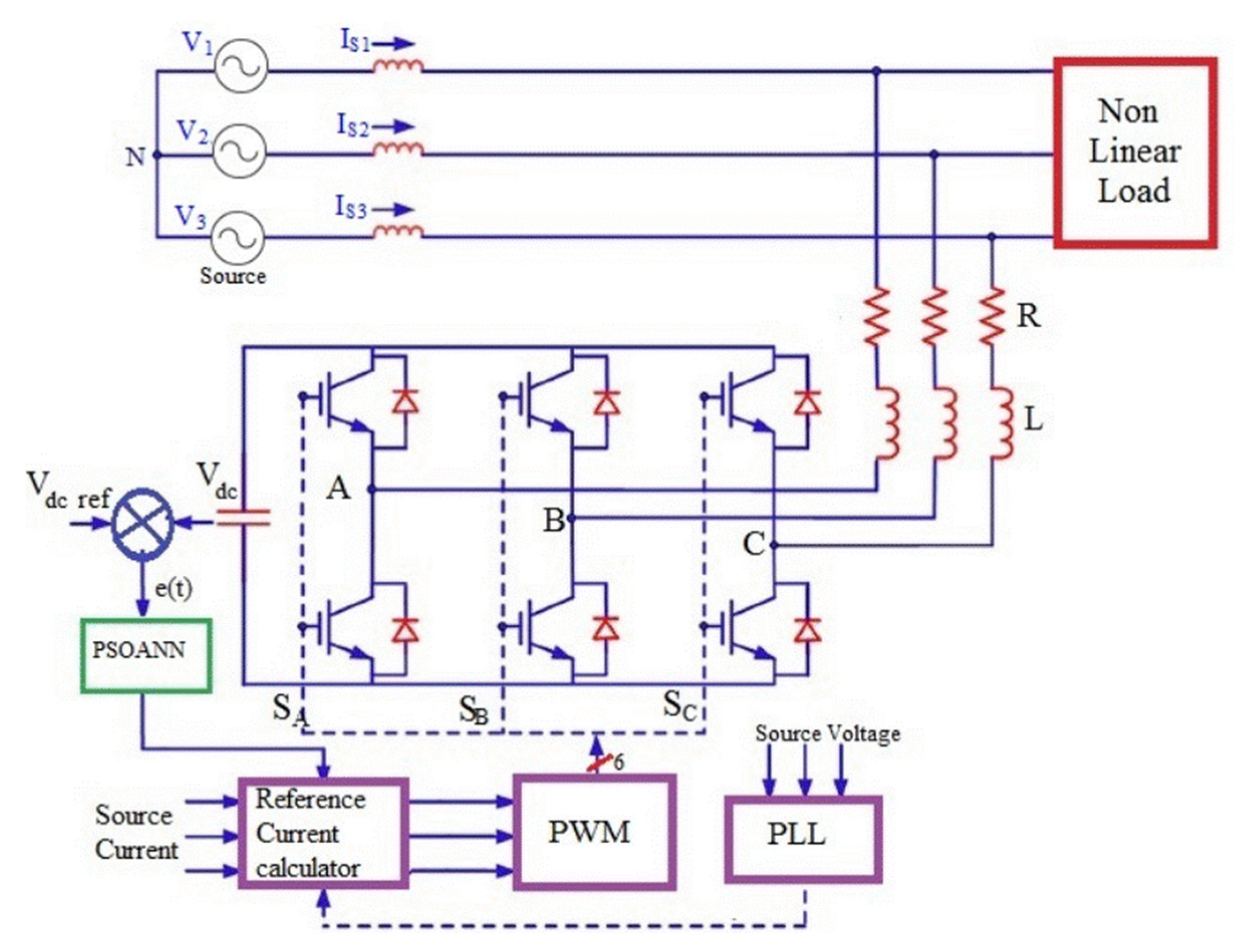
- Sujith, M.; Padma, S. Implementation of PSOANN Optimized PI Control Algorithm for Shunt Active Filter. Comput. Model. Eng. Sci. CMES 2020, 122, 863–888. [Google Scholar] [CrossRef]
- Djerboub, K.; Allaoui, T.; Champenois, G.; Denai, M.; Habib, C. Particle Swarm Optimization Trained Artificial Neural Network to Control Shunt Active Power Filter Based on Multilevel Flying Capacitor Inverter. Eur. J. Electr. Eng. 2020, 22, 199–207. [Google Scholar] [CrossRef]
- Abdedjebbar, T.; Zellouma Mohamed, T.; Benchouia Abdelbasset, K. Adaptive linear neuron control of three-phase shunt active powerfilter with an anti-windup PI controller optimized by particleswarm optimization. Comput. Electr. Eng. 2020, 96, 107471. [Google Scholar] [CrossRef]
- Ismael, K.S.; Kamal, S. Power quality improvement of distribution systems asymmetry caused by power disturbances based on particle swarm optimization-artificial neural network. Indones. J. Electr. Eng. Comput. Sci. 2022, 25, 666–679. [Google Scholar] [CrossRef]
- Patel, R.; Samal, P.; Panda, A.K.; Guerrero, J.M. Implementation of Bio-Inspired Flower Pollination Algorithm in Distribution System Harmonic Mitigation Scheme. In Proceedings of the 2021 1st International Conference on Power Electronics and Energy (ICPEE), Bhubaneswar, India, 2–3 January 2021; pp. 1–7. [Google Scholar] [CrossRef]
- Patel, R.; Samal, P. Performance analysis of bio inspired flower pollination algorithm based 3-phase shunt active power filter for dynamic condition in distribution system. Int. J. Syst. Assur. Eng. Manag. 2023, 2, 1–15. [Google Scholar] [CrossRef]
- Prince, S.K.; Panda, K.P.; Patowary, M.; Panda, G. FPA tuned Extended Kalman Filter for Power Quality Enhancement in PV integrated Shunt Active Power Filter. In Proceedings of the 2019 International Conference on Computing, Power and Communication Technologies (GUCON), New Delhi, India, 27–28 September 2019; pp. 257–262. [Google Scholar]
- Riad, N.; Anis, W.; Elkassas, A.; Hassan, A.E.-W. Three-Phase Multilevel Inverter Using Selective Harmonic Elimination with Marine Predator Algorithm. Electronics 2021, 10, 374. [Google Scholar] [CrossRef]
- Ranjan, S.; Jaiswal, S.; Latif, A.; Das, D.C.; Sinha, N.; Hussain, S.M.S.; Ustun, T.S. Isolated and Interconnected Multi-Area Hybrid Power Systems: A Review on Control Strategies. Energies 2021, 14, 8276. [Google Scholar] [CrossRef]
- Reddy, A.K.V.K.; Narayana, K.V.L. Optimal total harmonic distortion minimization in multilevel inverter using improved whale optimization algorithm. Int. J. Emerg. Electr. Power Syst. 2020, 21, 1–25. [Google Scholar] [CrossRef]
- Golla, M.; Chandrasekaran, K.; Simon, S.P. PV integrated universal active power filter for power quality enhancement and effective power management. Energy Sustain. Dev. 2021, 61, 104–117. [Google Scholar] [CrossRef]
- Lakshmi Kanthan Bharathi, S.; Selvaperumal, S. MGWO-PI controller for enhanced power flow compensation using unified power quality conditioner in wind turbine squirrel cage induction generator. Microprocess. Microsyst. 2020, 76, 103080. [Google Scholar] [CrossRef]
- Rao, B.C.; Sahu, P.; Jhapte, R. Comparative analysis of SRF based Shunt Active Filter using Grey Wolf and Eagle Perching Optimization. In Proceedings of the 2022 Second International Conference on Advances in Electrical, Computing, Communication and Sustainable Technologies (ICAECT), Bhilai, India, 21–22 April 2022; pp. 1–7. [Google Scholar] [CrossRef]
- Mishra, A.K.; Das, S.R.; Ray, P.K.; Mallick, R.K.; Mohanty, A.; Mishra, D.K. PSO-GWO Optimized Fractional Order PID based Hybrid Shunt Active Power Filter for Power Quality Improvements. IEEE Access 2020, 8, 74497–74512. [Google Scholar] [CrossRef]
- Almani, A.A.; Han, X.; Umer, F.; ul Hassan, R.; Nawaz, A.; Shah, A.A.; Mustafa, E. Optimal Solution for Frequency and Voltage Control of an Islanded Microgrid Using Square Root Gray Wolf Optimization. Electronics 2022, 11, 3644. [Google Scholar] [CrossRef]
- Alam, S.J.; Arya, S.R. Observer-based control for UPQC-S with optimized gains of PI controller. Int. Trans. Electr. Energy Syst. 2020, 30, e47233. [Google Scholar] [CrossRef]
- Manimegalai, M.; Sebasthirani, K. An Optimal Model for Power Quality Improvement in Smart Grid using Gravitational Search-based Proportional Integral Controller and Node Microcontroller Unit. Electr. Power Compon. Syst. 2022, 50, 989–1005. [Google Scholar] [CrossRef]
- Pattnayak, S.K.; Choudhury, S.; Nayak, N.; Bagarty, D.P.; Biswabandhya, M. Maximum Power Tracking & Harmonic Reduction on grid PV System Using Chaotic Gravitational Search Algorithm Based MPPT Controller. In Proceedings of the 2020 International Conference on Computational Intelligence for Smart Power System and Sustainable Energy (CISPSSE), Keonjhar, India, 29–31 July 2020; pp. 1–6. [Google Scholar] [CrossRef]
- Mishra, S.; Ray, P.K. Power quality improvement with shunt active filter under various mains voltage using Teaching Learning Based optimization. In Proceedings of the 2015 2nd International Conference on Recent Advances in Engineering & Computational Sciences (RAECS), Chandigarh, India, 21–22 December 2015; pp. 1–6. [Google Scholar] [CrossRef]
- Ali, S.; Bhargava, A.; Saxena, A.; Kumar, P. A Hybrid Marine Predator Sine Cosine Algorithm for Parameter Selection of Hybrid Active Power Filter. Mathematics 2023, 11, 598. [Google Scholar] [CrossRef]


| Harmonic Mitigation Techniques | 15 kW (Price) | 75 kW (Price) | 300 kW (Price) | THD-I (%) (Non-Linear Loads) | THD-I (%) (Mixed (50–50) Loads) |
|---|---|---|---|---|---|
| Reactor (5%) | 520 | 1100 | 3800 | 35 | 17.5 |
| Isolation Transformer | 2650 | 6340 | 18,000 | 35 | 17.5 |
| K-factor (13) Transformer | 5300 | 11,000 | 48,000 | 35 | 17.5 |
| Tuned Filter | 2800 | 3900 | 7000 | 12–20 | 3–12 |
| Low Pass Filter | 2400 | 5600 | 13,000 | 8–15 | N/A |
| Active Filter | N/A | 27,000 | 65,000 | 5 | 5 |
| Harmonic Limits a,b | TDD Required | |||||
|---|---|---|---|---|---|---|
| <20 | 4.0 | 2.0 | 1.5 | 0.6 | 0.3 | 5.0 |
| 20 < 50 | 7.0 | 3.5 | 2.5 | 1.0 | 0.5 | 8.0 |
| 50 < 100 | 10.0 | 4.5 | 4.0 | 1.5 | 0.7 | 12.0 |
| 100 < 1000 | 12.0 | 5.5 | 5.0 | 2.0 | 1.0 | 15.0 |
| >1000 | 15.0 | 7.0 | 6.0 | 2.5 | 1.4 | 20.0 |
| Bus Voltage (V) at PCC | Total Voltage Distortion THD (%) | Individual Voltage Distortion (%) |
|---|---|---|
| ≤8.0% | ≤5.0% | |
| ≤5.0% | ≤3.0% | |
| ≤2.5% | ≤1.5% | |
| ≤1.5% | ≤1.0% |
| Ref. | Years | Methodology | Feature | Result and Advantage | Disadvantage |
|---|---|---|---|---|---|
| [29] | 2019 | p-q theory | Power 3 phase | = 8.2%, Generate reference currents for modern power systems based on the steady-state variation of current and voltage vectors. | Unsatisfactory harmonic compensation efficiency less than 5% according to IEEE 519-2022 standard. |
| [29] | 2019 | DCAP method | = 3.5%, Divide the sinusoidal current into n parts and balance the source side. | Satisfactory harmonic compensation efficiency is less than 5% according to IEEE 519-2022 standard. | |
| [30] | 2019 | Predictive Direct Power Control (P-DPC) | = 1.2%, Maintain the DC bus offset voltage to a specified value and the anti-reverse compensated PI controller to regulate the DC bus voltage. | Effect of the sampling period and parameter error on power quality of distribution system. | |
| [31] | 2020 | LCL Filter | = 4.56%, The design is higher than the harmonic frequency compensation that the SAPF has to compensate for the higher order harmonics of the grid. | The control algorithm is complex. Resonance generation. The parameters of the LCL Filter are very complicated. | |
| [32] | 2020 | SiC-MOSFET | = 4.15%. Using the L-locator to suppress the switch sub-harmonics to a smaller level simplifies circuit design and control algorithms. The switching frequency is increased to 50 kHz. | Increases the second harmonic. | |
| [33,34] | 2020 | An ADALINE-based Neural Network (ANN) | = 2.39%, The current is measured using the Least Mean Square (LMS) algorithm; the weights are obtained with the help of online calculations. | Analysis under severe abnormal conditions is the direction of future research. | |
| [35] | 2021 | Space Vector Pulse Width Modulation (SVPWM) | = 3.73%, Trace and identify the reference voltage in a static coordinate system through coordinate transformation and determine the reference voltage. | The reference structure has only 4 transformation modes and no vector 0. This reduces the freedom of the composite vector and is difficult to control. | |
| [36] | 2021 | Triangle Orthogonal Principle (TOP) | = 4.98%, Using the phase signal from the phase-locked loop is synchronized with the grid signal based on the principle of triangle orthogonality. | Lack of selective harmonic compensation. | |
| [37] | 2021 | Computation Fluid Dynamics (CFD) | = 4.25%, Simulation of a heat transfer coupling under forced cooling conditions. | Designing power electronic components requires high precision. | |
| [38] | 2022 | Least Mean Square (LMS) | = 3.7%, Separation of the elementary active, reactive, and harmonic components of the distorted current. | Performance is low when using the same speed for components when estimating the feedback operation. | |
| [39] | 2022 | Modified Symmetrical Sinusoidal Integrator (MSSI) | = 3.94%, Extract the basic components of the corresponding forward sequence and use instantaneous reactive power theory to process the reference flow. | Look up the parameters of the transfer function. | |
| [40] | 2020 | Adaptive Backstepping Fuzzy Neural Controller based on Fuzzy Sliding Mode (FNN-based FSM) | Power 1 phase | = 4.48%, Establish a subsystem and use virtual controls to simplify controller design. | Satisfactory harmonic compensation efficiency is less than 5% according to IEEE 519-2022 standard. |
| [41] | 2021 | Long and Short Term Memory Fuzzy Neural Network (LSTMFNN) | = 4.67%, Combine fuzzy neural network and long and short-term memory mechanism to enhance self-learning ability and high performance. | Improve control effect, new neural network learning strategies, finite time control and reduction of system chattering are future research directions. | |
| [42] | 2022 | Modified Multiport Interleaved Flyback Convertor (MMPIFC) | Photovoltaic (PV) three-phase power | = 2.61%, Multi-port interlaced flyback conversion to connect n number of input sources to DC bus to overcome partial shadow problem. | Replacing fuzzy controls with advanced artificial intelligence algorithms like bio-inspired optimization is the direction of future research. |
| Step | Step-By-Step Explanation of the GA Method |
|---|---|
| Step 1: | Determining the ranges of the parameters; the upper and lower bound |
| Step 2: | Set the value |
| Step 3: | Set population size |
| Step 4: | Set the initial population by random within the space of parameters |
| Step 5: | Set maximum numbers of generations |
| Step 6: | Set the selection process following the tournament method, mutation, and crossover |
| Step | Step-By-Step Explanation of the ABC Algorithm Method | |
|---|---|---|
| Step 1: | Parameters are set like colony number, size, the value of limits, restrictions and maximum number of cycles for foraging | |
| Step 2: | , with constraints set up for each bee at random (Equation (7)). | |
| (7) | ||
| Step 3: | The function value is established (Equations (8) and (9)) | |
| (8) | ||
| (9) | ||
| : The i-th root obtained in the cost function. | ||
| Step 4: | Establish a foraging process for hired bees, observers and scout bees. There, the role of the hired bees is to search and evaluate the quality of the found food source; if the food source is unsatisfactory, they store it in memory and start looking for a new and better food source, and they divide this information to the observer bees in the hive. | |
| Step 5: | bees observe, receive information, evaluate the information received and choose a quality food source. They then pass the information back to the swarm, and together they rate the quality of the nectar and compare it to the quality of the previous nectar. Where the quality of the nectar is better than the quality of the previous nectar, they switch to a source with better quality nectar. At the same time, they also change the memory of the old nectar information (Equation (10)). | |
| (10) | ||
| With, i: is the i-th food source. P(i): Probability that the observed bee chooses a food source. | ||
| Step 6: | The old food source is also removed and improved with a new food source after each establishment, and this work is performed by scout bees. | |
| Step 7: | Loop when reaching the maximum value, the algorithm terminates. Otherwise, the loop is updated next with the formula iter = iter + 1 and goes back to step 4 to continue executing the program. | |
| Step 1: | (Parameter Initiation) | |
| End | ||
| Step 2: | (Local Update Rules) | |
| with a transition probability given in Equation (12). | ||
| Calculate cost k | ||
| End | ||
| For k = 1 to m | ||
| For k = 1 to m | ||
| Update the pheromone using Equation (11) | ||
| End | ||
| End | ||
| Step 3: | (Global update rules) Update pheromone for best and worst tours of ant using Equations (11) and (12). | |
| Globally update pheromone using Equation (16) | ||
| Tour = tour + 1 | ||
| If (tour < maximum tour) | ||
| Go to step 2 | ||
| Else | ||
| Print the best node values for the minimum cost function | ||
| End | ||
| Step | Step-By-Step Explanation of the ABC Algorithm Method | |
|---|---|---|
| Step 1: | Establish the function of the bat according to the formula F. | |
| Step 2: | Initialize functional variables, including upper bound information and lower bound information of each bat, number of bats, maximum number of repetitions, and number of variables looking for food sources. Each bat has different upper and lower bound parameters in the foraging zone. | |
| Step 3: | Call and Find the initial value of the objective function | |
| Step 4: | The maximum number of repetitions is to be performed from the start of the main loop, and the frequency is randomly chosen according to Formula (30). | |
| (30) | ||
| Step 5: | Update the speed and position of the bat. After each update of the upper and lower bound values, the new position of the bat is updated according to Formula (31). | |
| (31) | ||
| Step 6: | Check the pulse rate of each bat. The random step size limiting factor is 0.001. | |
| Step 7: | Recalculate the fitness value after optimization according to Formula (32). Plot the convergence curve for the best fit and repeat. The best position is also called the optimized value. | |
| (32) | ||
| Step | Step-By-Step Explanation of the BFO Algorithm Method | |
|---|---|---|
| Step 1: | (Chemotaxis): bacteria move to find a source of more nutrients in the intestines thanks to the mechanism of bladder action in directions such as swimming or somersaults. Assume is the ith bacterium in the jth trophic zone, the kth spawning zone, and the lth elimination dispersal step. The bacteria in motion were calculated according to Formula (34). | |
| (34) | ||
| where C(i) is the size of a single step and movement in a random direction, and Δ(i) is the vector in an arbitrary direction of the elements in the range [−1, 1]. | ||
| Step 2: | (Swarming): bacteria move in swarms with high density in the activity of sourcing nutrients through mechanisms of attracting and repelling substances given by Formula (35). | |
| (35) | ||
| are measures of the number, rate of diffusion, and strength of the forward and backward effects of bacteria, respectively. | ||
| Step 3: | (Reproduction): the acclimatization value of bacteria i in NC migration and calculated according to Formula (36). | |
| (36) | ||
| is the health of the representative ith bacterium. The healthy bacteria eventually eliminate other healthy bacteria, and the population stays the same in the end. | ||
| Step 4: | after the Nre spawning event with the goal that the bacteria are not trapped and ensure that the local optimum replaces the global optimal. The objective function is optimized following Formula (37). | |
| (37) | ||
| is the steady-state time of the transition period. | ||
| Step | Step-By-Step Explanation of PPFO Algorithms | |
|---|---|---|
| Step 1: | Read the problem data | |
| Step 2: | ||
| Step 3: | Generate the initial population of fireflies as represented by Equations (38) and (39) | |
| Step 4: | ||
| While termination requirements are not met, do | ||
| firefly as a design parameter in the Simulink model of SAPF. | ||
| Run the Simulink model and compute THD | ||
| using Equation (40) | ||
| firefly as a design parameter in the Simulink model of SAPF. | ||
| Run the Simulink model and compute THD | ||
| using Equation (40). | ||
| using Equation (42). | ||
| using Equation (41). | ||
| firefly through Equation (43). | ||
| End if | ||
| If rand < n?. | ||
| firefly using Equations (44) and (45). | ||
| End | ||
| End-(i) | ||
| End-(j) | ||
| Rank the fireflies and find the current best and worst fireflies. | ||
| End-(while) | ||
| The firefly possessing the largest brightness is the optimal solution. | ||
| Step | Step-By-Step Explanation of ASNS Algorithms |
|---|---|
| Step 1: | is updated after each iteration |
| Step 2: | |
| Step 3: | The objective function value of ASNS is compared to step 2 and updated at the first corner starting from the left of the hexagon |
| Step 4: | and replaces the objective function. Then, turn back to step 3 |
| Step 5: | If the value meets the optimal level, ASNS is selected as the optimal solution and saved in the best solutions list |
| Step 6: | . Then, update the objective function and reperform step 3 |
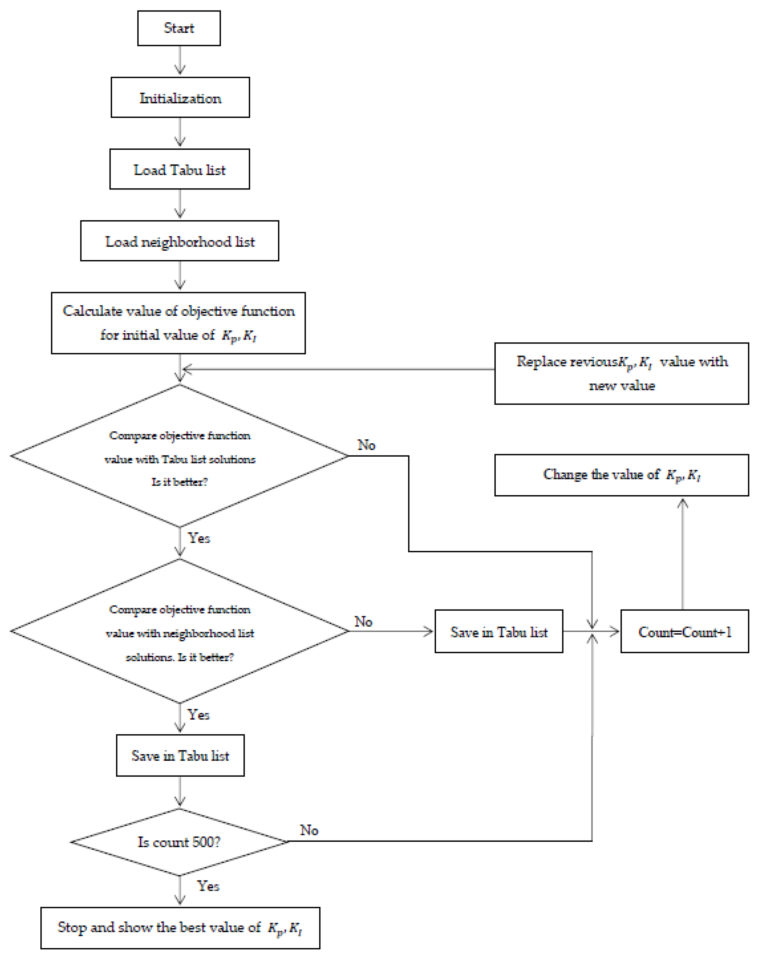
| Step | Step-By-Step Explanation of ATS Algorithms |
|---|---|
| Step 1: | Initialize Tabu TL and count values to 0 |
| Step 2: | is the best neighbor |
| Step 3: | is the set of N solutions |
| Step 4: | , then choose the optimal value and assign it to the best neighbor 1 |
| Step 5: | as thebest neighbor. In addition, set the best neighbor 1 in TL |
| Step 6: | Evaluate the last criteria (TC) and the aspiration criteria (AC). If count max = count (the maximum number allowed in the search area), stop the search process. The current best solution is the best overall solution. If not, go back to step 2 and continue the process |
| Step | Step-By-Step Explanation of ATS Algorithms | |
|---|---|---|
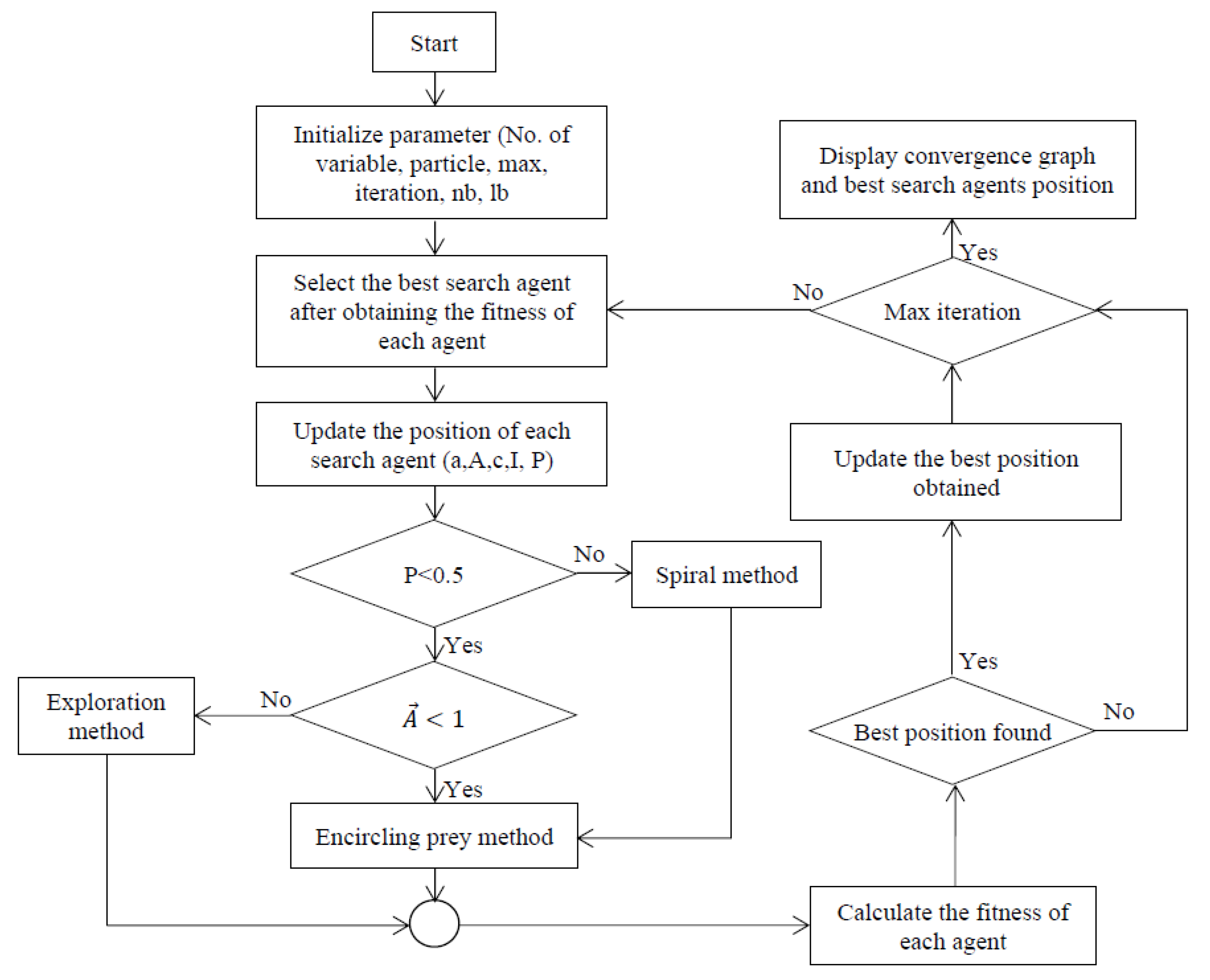
| Step 1: | At first, the whale acquaints itself with the prey, then surrounds the prey. The whale predicts the best solution and calls it objective prey and is substituted when there is another better solution. Variables are updated according to the Formulas (47) and (48). | |
| (47) | ||
| (48) | ||
| are updated by Formulas (49) and (50) | ||
| (49) | ||
| (50) | ||
| = random vector between [0, 1]. | ||
| Step 2: | Exploitation phase, whales will attack their prey with a bubble net strategy and do so with twomethods, including shrinking, encircling, and spiral updating. Spiral is shown according to Formulas (51) and (52). | |
| (51) | ||
| (52) | ||
| whale compared to the best updated solution. L = random number in [−1,1], b = fixed number for the spiral algorithm. The algorithm model is built as Formula (53). | ||
| (53) | ||
| where the random value of p is selected in [0, 1] . | ||
| Step 3: | vector number is selected randomly to update the search location and perform according to Formulas (54) and (55). | |
| (54) | ||
| (55) | ||
| = random vector chosen from whales’ location from the current population. After applying WOA and SAPF, the THD = 1.49%, within the IEEE 519-2022 standard, where the objective function is according to Formula (56). | ||
| (56) | ||
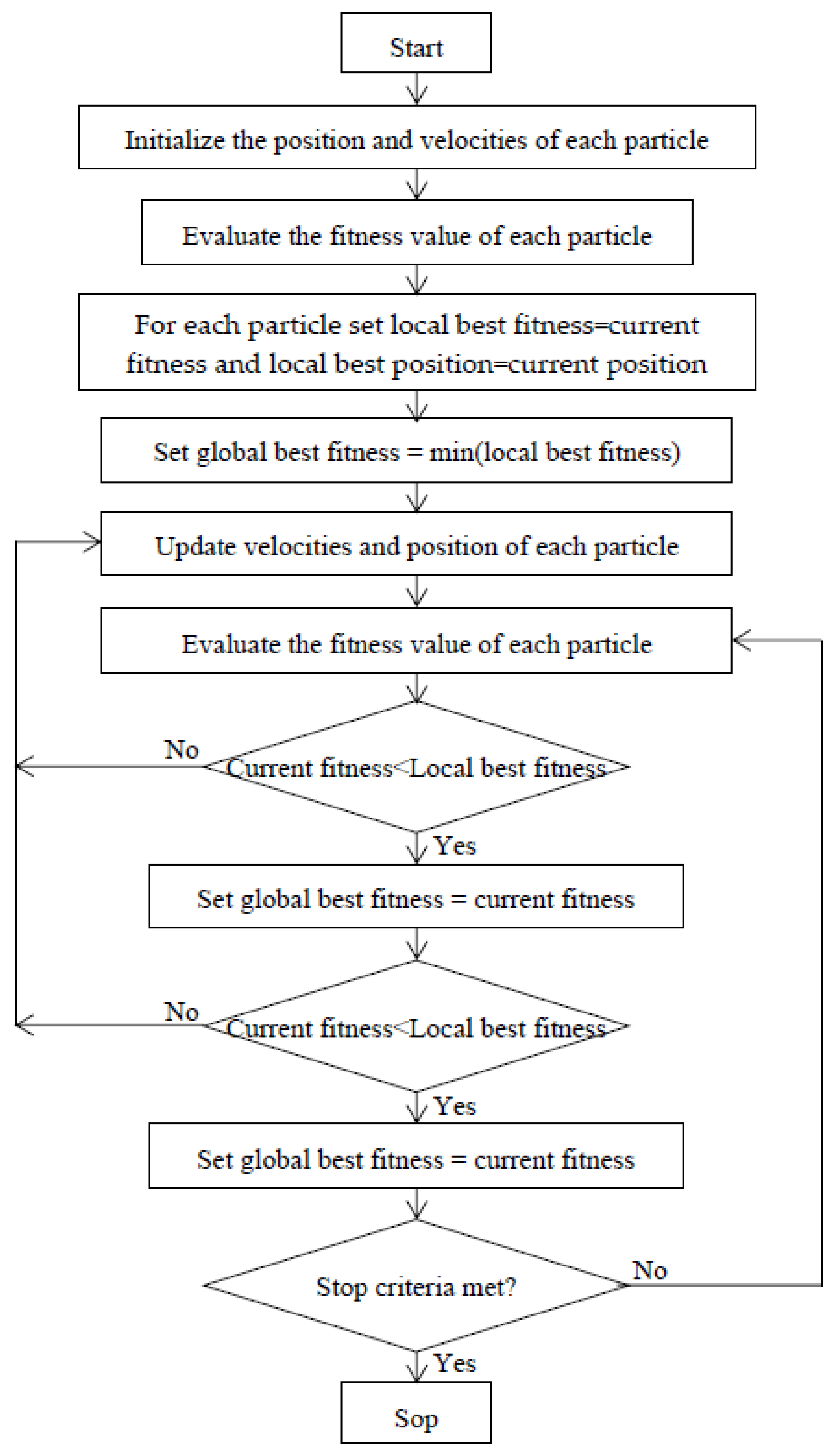
| Step | Step-By-Step Explanation of PSO Algorithms | |
|---|---|---|
| Step 1: | , find the current fitness of each particle in the population. | |
| Step 2: | of each county at their respective current position according to Formula (60). | |
| (60) | ||
| Step 3: | The global best fitness value is calculated according to Formula (61) | |
| (61) | ||
| . | ||
| Step 4: | Update the position and velocity of the particles according to Formulas (62) and (63). | |
| Step 5: | and find the current fitness of each particle. If current fitness < local best fitness, set. | |
| (62) | ||
| (63) | ||
| Step 6: | loop is calculated as follows: | |
| (64) | ||
| If current global best fitness < global best fitness, then. | ||
| (65) | ||
| . | ||
| Step 7: | Repeat steps 5 and 6 until k is equal to the maximum value of the loop defined in step 1 or there is no global best fitness improved. | |
| Step 8: | End the algorithm loop or until no more loops are executed | |
| Step | Step-By-Step Explanation of ANN Network Algorithms | |
|---|---|---|
| Step 1: | The training network generates a control pulse (z) with a time interval (t) input | |
| Step 2: | is made using Formula (72) | |
| (72) | ||
| Step 3: | The above equation is the output of the network. | |
| (73) | ||
| where a is a function node deviation of one or two and n | ||
| Step 4: | The weight of each neuron is calculated using Formula (74). | |
| (74) | ||
| Step 5: | Weight adjustment is calculated as follows: | |
| (75) | ||
| Step 6: | All above steps repeat until LMBP min (LMBP < 1) | |
| Rule | Explanation of the FPA Algorithm’s Rules | |
|---|---|---|
| Rule 1: | Pollen and the best global solutions are defined by Formula (76) | |
| (76) | ||
| is the most recent best pollen with oneset of pollen. L = represents theLevy factor that is responsible for the movement of the pollen group, and this factor follows the Levy distribution and is calculated using Formula (77) | ||
| (77) | ||
| Rule 2: | The equation for local pollination or self-pollination, following Formula (78) | |
| (78) | ||
| is a random number in the range 0–1. | ||
| Rule 3: | , make the transition from local to global search, and a p-value = 0.8 often gives the optimal result. | |
| Step | Step-By-Step Explanation of FPA Algorithms | |
|---|---|---|
| Step 1: | ||
| Step 1: | Main FPA algorithm | |
| First of all, the first decision variable is chosen randomly in the lower and upper bounds, as shown in the flowchart below. | ||
| For i = 1:n; | ||
| ; | ||
| End | ||
| Next, identify the fitness or error of the first population and do the following flowchart. | ||
| For i = 1:n; | ||
| End | ||
| Where CF = current fitness and PIC is a function that combines the Matlab and Simulink models of SAPF. Normally, CF is in 50 × 1 size | ||
| In the next step, pollen is updated according to rules 1 and 2, and the probability p-value is randomly selected in the range 0–1. If the random number is greater than p, then the pollen value is calculated according to Formula (79) | ||
| (79) | ||
| Provide by rule 1. On the other hand, if the random number is less than p, then the pollen obeys rule 2 | ||
| Evaluate the fitness value after updating the pollen value according to the following equation. | ||
| For I = 1:n | ||
| = PIC(x.u(i)); : updated value of fitness and x.u: updated pollen value | ||
| End | ||
| Updating the current global best fitness value from local best fitness is described in detail by the following equation | ||
| If CFU < CF | ||
| BESTP = PIC(x()i); | ||
| CF = CFU | ||
| End | ||
| These steps are repeated until the value of the mathematical equation reaches convergence and the iteration becomes more than the maximum number of iterations initially set; then, the program is stopped. | ||
| flower pollination value achieved with the minimum error value | ||
| Step | Step-By-Step Explanation of the GSA Algorithms | |
|---|---|---|
| Step 1: | The position of the third agent in the N agents is determined by Formula (88) | |
| (88) | ||
| dimension; N: the size of the search space. | ||
| Step 2: | At time t, the i-th force is applied from the j-th, and this applied force is calculated by Formula (89) | |
| (89) | ||
| : euclidean distance between regions i and j. | ||
| Step 3: | The total force acting on i in the dimension d over time t is calculated by Formula (90) | |
| (90) | ||
| : first K-zone with the best fitness value. | ||
| Step 4: | Acceleration relative to mass i in time t in terms of size d is calculated by Formula (91) | |
| (91) | ||
| : mass of inertia of agent i | ||
| Step 5: | The next velocity of space is a fraction of the current velocity plus its acceleration. The position and velocity of the agent are calculated according to Formulas (92) and (93) | |
| (92) | ||
| (93) | ||
| Step 6: | The weight constant (G) is first set at the start of the search, and its value is decreased over time to achieve the goal of controlling accuracy when searching in the search space and following Formula (94) | |
| (94) | ||
| and a: constants. | ||
| Step 7: | Gravitational mass and initial mass are updated according to Formulas (95)–(97) | |
| (95) | ||
| (96) | ||
| (97) | ||
| : fitness value of region i at time t. | ||
| Step 8: | : the minimum and best value of the problem is calculated by Formulas (98) and (99). | |
| (98) | ||
| (99) | ||
| Ref. | Method | Results and Benefits of Applying Meta-Heuristic Optimization to SAPF | Limitation or Future Research |
|---|---|---|---|
| [67,68,69,70] | DE | Improve turning of the proportional-integral control loop of SAPF. The THD value reaches 3.42% to meet the IEEE 519-2022 standard. | The meta-heuristic hybrid method is different from DE; the aim is to reduce the THD value to meet the IEEE 519-2022 standard. |
| [71,72,73,74,75,76,77] | GA | Controller turning to obtain optimum gain values to switch SAPF and THD in the supply current present in the hardware is 1.4%, more than the simulation results of 1.24%. | Control technique for the SAPF system with time-varying parametric uncertainties. |
| [78,79,80,81,82] | ABC | To solve the nonlinear equation of selective harmonic elimination patterns considering unequal direct current sources, satisfying fundamental components, and eliminating low-order harmonics. The THD of the hardware is 11.78%, more than the simulation results of 10.46%. | Propose a hybrid method that combines meta-heuristics and ABC to reduce THD and meet the IEEE 519-2022 standard. |
| [83,84,85,86,87] | ACO | Optimize the gain values of the PI controller used in SAPF. The setting time (Ts) is 28 ms, and the THD of the supply current is 3.85%, 2.92%, and 3.49% for phase a, phase b, and phase c, respectively. | Consider the proposed systems to be an efficient solution to the growing demand forpower at the present and in the future. |
| [88,89,90,91] | ALO | To properly tune the circuit in order to reduce the harmonics in the source current and load voltages, the THD of the supply current with RL load is 3.73%, and the RLC load is 4.03%. The THD of the supply voltage with RL load is 4.2%, and the RLC load is 4.44%. | The technique works for different load variations in the system. |
| [92,93,94] | BA | Proportional resonant controller-based pulse width modulation. Current control for three-phase, three-leg SAPF with the optimized DC-link controller. The THD value reaches 0.7% to meet the IEEE 519-2022 standard. | BA is very promising for solving other multi-objective optimization problems. |
| [95,96,97] | BFO | To optimize the parameters of the PI controller through an online self-adaptive self-turning algorithm. The THD value reaches 1.9% to meet the IEEE 519-2022 standard. | BFO-based SAPF proves to be a significant approach to reducing the ripple current harmonics. |
| [98,99,100,101,102,103,104,105,106] | FA | Optimization problems with the objective of minimizing the THD and solving it using predator-prey-based firefly optimization. The THD is 1.9092%. | The proposed method can be extended to designing hybrid active power filters in future works. |
| [107,108] | ASNS | The optimization of conventional control scheme used in SAPF. THD of supply current is 1.21%, 1.14%, and 1.11% for balanced, unbalanced, and distorted loads, respectively. Compensation time (Ts) is 0.055 (s), 0.003 (s), and 0.001 (s) for balanced, unbalanced, and distorted loads, respectively. | Design for all different types of HAPF. |
| [109,110,111,112] | TS | The instantaneous power theory with Fourier and the optimal design of the current predictive controller. The THD of the supply current is 0.96%. | The proposed novel active filter can be applied to higher-frequency systems. |
| [113,114,115,116,117,118,119] | WOA | ). The THD of the supply current is 3.07% | A tuned PI controller can be used in hardware for real-time implementation. The proposed modern industrial optimization should be tested under various range constraints by using new techniques to handle the constraints. |
| [120,121,122,123,124,125,126,127,128,129,130,131,132,133] | PSO | The selection of a proper reference compensation current extraction scheme plays the most crucial role in the performance of SAPF and includes conventional instantaneous active and reactive power (p-q),modified p-q, and instantaneous active and reactive current component (id-iq) schemes.THD of supply current is 3.45%, 2.97%, and 3.07%, based on phase a, phase b, and phase c, respectively. | A hybrid method that combines other meta-heuristic methods into the search area of PSO to help limit the fast convergence error of PSO, such as DE-PSO, GA-PSO, and Levy-flight-PSO. |
| [133,134,135,136,137,138] | FPA | To maintain the DC link voltage constant, the proportional-integral (PI) controller being employed on the DC side of SAPF is used to minimize the error between voltage and actual value. The THD of the supply current is 3.13%, and Ts is 0.001 s. | Application of some hybrid optimization algorithm for the determination of optimal controller parameters. |
| [139,140,141,142,143,144] | GWO | To reduce the maximum overshoot and undershoot of the DC-link voltage variation and minimize power ripples with current distortion in IEEE 519-2022. Improve the predictive direct power control of three-phase SAPF. The THD of the supply current is 3.8% and 57%, based on simulation and experimental data, respectively. | Propose a hybrid method that combines meta-heuristics and GWO to enhance work efficiency. |
| [145,146] | GSA | The harmonic content reduction in the source current is carried out with optimal turning of the PI controller. The THD of the supply current is 1.76%. | Propose a hybrid method that combines meta-heuristics and GSA with the aim of maximizing work efficiency. |
| [147,148,149,150] | TLBD | The reference current signals are generated by sensing the source voltage load current and DC bus voltage; with these signals, the gate driving pulses are generated by a band current controller. THD of the supply current is 1.06%. | Propose a hybrid method that combines meta-heuristics and TLBO to maximize productivity. |
Disclaimer/Publisher’s Note: The statements, opinions and data contained in all publications are solely those of the individual author(s) and contributor(s) and not of MDPI and/or the editor(s). MDPI and/or the editor(s) disclaim responsibility for any injury to people or property resulting from any ideas, methods, instructions or products referred to in the content. |
© 2023 by the authors. Licensee MDPI, Basel, Switzerland. This article is an open access article distributed under the terms and conditions of the Creative Commons Attribution (CC BY) license (https://creativecommons.org/licenses/by/4.0/).
Share and Cite
Duc, M.L.; Hlavaty, L.; Bilik, P.; Martinek, R. Harmonic Mitigation Using Meta-Heuristic Optimization for Shunt Adaptive Power Filters: A Review. Energies 2023, 16, 3998. https://doi.org/10.3390/en16103998
Duc ML, Hlavaty L, Bilik P, Martinek R. Harmonic Mitigation Using Meta-Heuristic Optimization for Shunt Adaptive Power Filters: A Review. Energies. 2023; 16(10):3998. https://doi.org/10.3390/en16103998
Chicago/Turabian StyleDuc, Minh Ly, Lukas Hlavaty, Petr Bilik, and Radek Martinek. 2023. "Harmonic Mitigation Using Meta-Heuristic Optimization for Shunt Adaptive Power Filters: A Review" Energies 16, no. 10: 3998. https://doi.org/10.3390/en16103998