Influence of the Longitudinal and Tree-Shaped Fin Parameters on the Shell-and-Tube LHTES Energy Efficiency

Abstract

Changes in the energy sector, associated with the move away from fossil fuels, pose a challenge for appropriate thermal energy management in residential buildings. The important element to deal with the variability of renewable energy in thermal systems is latent heat thermal energy storage. Due to the low thermal conductivity of phase change materials, a number of techniques are proposed to enhance the heat transfer process. In this research, the global sensitivity of fin geometrical parameters on the melting and solidification times and energy efficiency of these processes was investigated. The computational model of the phase change was developed using the finite volume method with the enthalpy-porosity model and Boussinesq approximation. Numerical simulations were carried out according to the design of experiments technique. The multi-dimensional response surface was developed, and the multi-objective optimisation was done. The research shows that the melting process is most influenced by the position of the top fin ($\alpha$ angle) and the solidification process by the position of the bottom fin ($\gamma$ angle). The angle of the tree fin ($\beta$) has a different effect on both processes, with the energy efficiency decreasing during melting and increasing during solidification. Maximum values for the energy efficiencies of melting (${\eta }_m=0.973$) and solidification (${\eta }_s=0.988$) were obtained for $\alpha =18.2^{°}$, $\beta =89.0^{°}$, $L=10.7$ mm and $\gamma =21.0^{°}$.

1. Introduction

In relation to energy transformation, the topic of changes in the thermal management of buildings is coming up more and more frequently. Over the past decades, the increasing use of renewable energy sources requires a solution to the problem of optimal energy generation, conversion and storage. Taking additionally into account the need to match the efficiency of the energy source with the fluctuating energy demand, Thermal Energy Storage (TES) could soon become one of the main energy supply chains components from Combined Heat and Power (CHP) plants, as well as facilitating private prosumers’ move towards energy independence.

TES technology stands at various stages of development. Sensible Heat TES (SHTES), which uses the specific heat capacity of a medium by changing its temperature, is the current solution [1]. Storage units based on reversible endothermic and exothermic reactions are under research and development. On the other hand, Latent Heat TES (LHTES), which utilises the heat of phase change, is becoming increasingly popular [2]. The shell-and-tube unit is among the most commonly developed designs for TES purposes. In these systems, Phase Change Materials (PCMs) are usually placed in the space between the tube and enclosure [3]. Heat Transfer Fluid (HTF) flows through the pipe in case of TES charging or discharging. Nowadays, PCMs are being used more extensively in climate-controlled floor and ceiling systems, server rooms and data centres [4]. PCMs have also found applications in the construction [5], transport [6], electronics, medical, pharmaceutical, and agricultural industries [7]. 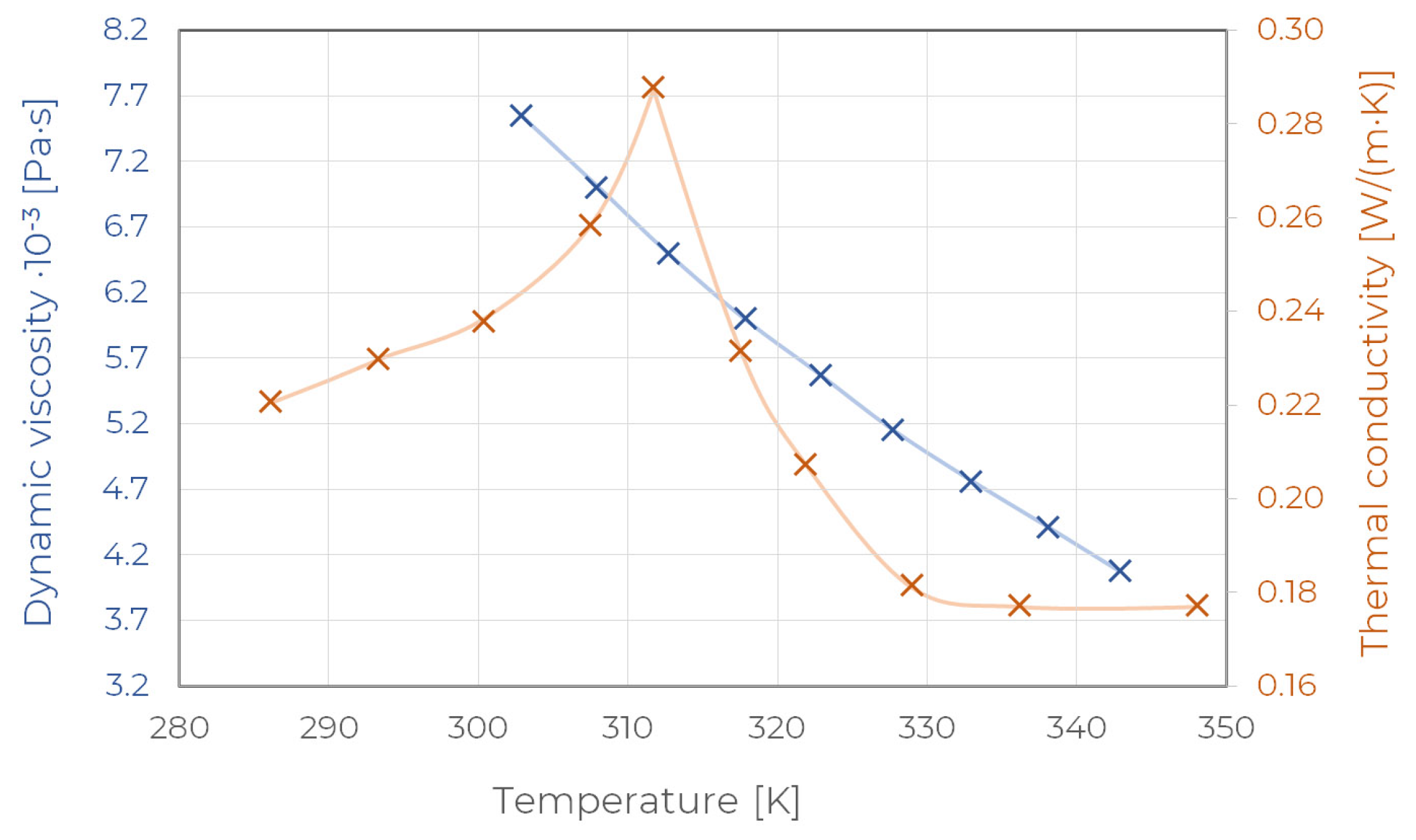Considering the high energy density of the PCM [8], it is expected that it will be used to create compact and economical TES. However, the main disadvantage associated with the implementation of efficient solutions based on PCM is their low thermal conductivity [9]. Rathore and Shukla [10] noted that the thermal conductivity of the majority of organic PCMs is typically between 0.18 and 0.3 W/(m · K), whereas for molten salts [11] these values are in the range 0.5–1.8 W/(m · K) Consequently, over the past few decades, attention has turned to heat transfer enhancement methods. In principle, three general methods were studied: augmenting the effective thermal conductivity of the PCM [12], increasing heat transfer surface area [13] and improving the process uniformity [14].

Among the techniques to improve the effective thermal conductivity of PCM is to insert additives [15,16]. One of the most popular additives are carbon-based materials, because of their high thermal conductivity, stable thermal and chemical properties and good compatibility [17]. Due to the many challenges in the application of these materials, metal-based additives such as nickel foam, silver nanowire [18], copper nanoparticles [19] or paraffin–nanomagnetite composites [20] are increasingly being used [21]. However, metal-based additives are affected by a number of limitations in practical implementations due to their high density, difficulty in uniform dispersion (resulting in unstable heat transfer), and high reactivity with other substances [22].

The second way to enhance heat transfer in LHTES is to increase heat transfer surface area, and it has received significant research attention. Different methods have been investigated for this purpose, including fins [23], shell and tube geometry modification [24], using embedding heat pipe [25], using multi-tube heat exchangers [26], micro-encapsulation [27], nano-encapsultaion [28].

Although researchers have explored various innovative methods to improve the efficiency of PCM applications, the method of using extended surfaces such as fins is one of the most commonly used methods because of its simplicity. Moreover, a common construction option for LHTES is horizontally oriented shell-and-tube systems [29].

In LHTES systems, straight longitudinal fins are frequently used. The effect of fin geometric parameters on charging performance has been studied many times. The results show that melting time decreases as the number [30], length, and thickness of the fin increase [31], due to an enlargement of the heat transfer surface area.

Research has pointed out that natural convection has the main influence on PCM melting. In the early stages of this process, heat transport by conduction has a dominant contribution, but over time the effect of natural convection becomes more pronounced [32]. Considering previous observations, the placement of the fins in the lower part of the horizontal shell and tube unit is more effective in reducing the total melting time [33]. Such an arrangement of the fins prevents blockage of convection currents. However, the placement of an excessive number of fins leads to suppression of the induced natural convection [34]. A study by Khan and Khan [35] considering the influence of angular orientations of the fins showed that the fins at the top, especially in the vertical axis of the cross-section is undesirable which is supported by the results of melting time and the overall energy capacity of LHTES. Investigations into the effect of geometric parameters of the fins, with their volume, held constant, are proving important. In the study developed by Yang et al. [36], it turns out that increasing the number of fins while keeping their volume constant, does not always lead to a reduction in melting time. The total melting time decreases as the number of fins increases to the optimal value of 52 in this study. In another work, Nie et al. [37] noted that a smaller number of long fins is more efficient when it comes to enhancing the rate of phase change than a larger number of short fins. The research results of phase change studies in a rectangular box [38] showed that long upper fins and short lower fins usually suppress convective cells. The opposite condition intensifies natural convection and reduces phase change time. In addition, by lengthening and thickening the lower fins while shortening and thinning the fins in the upper part of the LHTES cross-section, the melting time is reduced by 54.1% in comparison with the base case [39]. Yu et al. [40] used the appropriate gradients of fin thickness and noted that the central angle promotes the reduction in melting time by up to 30.5%. Therefore, it is recommended that the fin configuration be spaced with a gradient angle and thinner at the top and thicker at the bottom of the LHTES unit. In the cited studies, the effect of one geometric parameter on the melting process is investigated, while the others are unchanged. When one parameter is modified, the effect of the other on the investigated value may already be different. Furthermore, the simulations determined the melting time at specific points, while the character of the relationship over the entire range of parameter changes is unknown.

During solidification, on the other hand, convection dominates at the beginning, when the contribution of the liquid phase is significant, and conduction is prevalent when there is sufficient solid PCM in the LHTES unit. Nobrega et al. [41] examined the influence of geometric parameters that include the number and fin width. The results demonstrated that an increase in the number and the width of the fins reduces the total solidification time. However, there is an optimal number of fins and an optimal fin width above which there is no significant reduction in the total phase change time. Shahsavar et al. [42] showed that the use of a uniform fin arrangement in an LHTES unit can reduce solidification time by 9.7%. The minimisation of melting time is more pronounced with a reduction of 41.4%. Li and Wu [43] found that the use of the fins allowed the device to increase performance and accelerate melting and solidification processes by 14%. The use of fins at the bottom of the LHTES unit, which leads to an improvement in the melting time, contributes to a delay in the solidification process. Increasing the length of the fins and their number, with an even distribution, is more effective for solidification than for melting [37]. The thickness of the fins, on the other hand, is a parameter that does not have a significant effect on the time of the solidification process [44].

To further improve solidification and melting performance, a number of innovative fin shapes have recently been proposed, including triangular [45], corrugated [46], V-shaped [47], exponential [48], spider web-shaped [49], snowflake-shaped [50], tree-shaped [51], Y-shaped [52], longitudinal triangular fin [53], circular superimposed longitudinal fin [54] structures. Sarani et al. [55] proposed a novel configuration of discontinuous fins that resulted in an 89% reduction in discharge time. Al-Mudhafar et al. [56] observed that the total phase change time was decreased by 33% with the tee fins, relative to the implementation of longitudinal fins. Pahamli et al. [57] designed a novel LHTES with a set of Blossom-Shaped Fins (BSFs). Increasing the number of fins by addition of five BSFs to the LHTES unit, extends the melting time by 6%. Reducing the height of the fins from 28 mm to 24 mm significantly improves the melting process, but prolongs the final stage of phase change. It is worth noting that the shape of some of the proposed fin types is difficult to manufacture, which affects the cost–effectiveness of TES. Many numerical studies are also limited to investigating the influence of only one parameter while the values of the others are constant. Moreover, the interactions between all geometrical parameters are neglected.

Many approaches have been used to analyse heat transfer in LHTES units. Empirical research has been carried out on laboratory stations [58]. Despite its many advantages, there is often a need to carry out experiments on many different designs, which is associated with an increase in the cost of the testing time. Huang et al. [59] developed and compared two approximation-assisted reduced-order LHTES models. The mathematical model of solid-liquid and liquid-solid phase change in the form of partial differential equations has also been proposed many times. Among other things, they were solved using the standard finite element method, the Galerkin formulation [60]. A significant number of publications focus on the application of the finite volume method [42,61] using the enthalpy-porosity method. This approach involves solving the Navier-Stokes equations. The Lattice-Boltzmann Method, on the other hand, as an explicit approach with second-order accuracy, allows the use of molecular motions to determine macroscopic properties [62]. Many methods have been used to optimise the system and to develop a surrogate model, including the Adaptive-Kriging-High dimensional model representation (HDMR) method [63]. Sensitivity analysis and optimisation of the LHTES system were carried out using the multi-objective particle swarm optimisation (MOPSO) method and multiple attribute decision-making (MADM) algorithm [64]. Among the methods used to determine the response surface in LHTES systems, Genetic Aggregation [65] and Kriging’s method [66] are also used. The distribution of fins and phase-change material in the TES has also been obtained using topology optimisation [67]. What is more, machine learning in combination with numerical simulation is increasingly being used by researchers [68].

Based on the literature review, it was concluded that the fin arrangement in LHTES has a significant impact on melting and solidification times and optimisation of geometrical parameters is becoming an important part of the process of developing efficient designs. The majority of authors investigate the influence of individual geometrical parameters based on one factor at a time experiment, while the influence of interactions between input parameters is often neglected. Furthermore, the value of the energy efficiency during the melting and solidification process, which is important for the evaluation of the LHTES system, is rarely determined. Only a few publications carry out a multi-objective optimisation of the geometrical parameters of the LHTES system taking into account both solidification and melting processes.

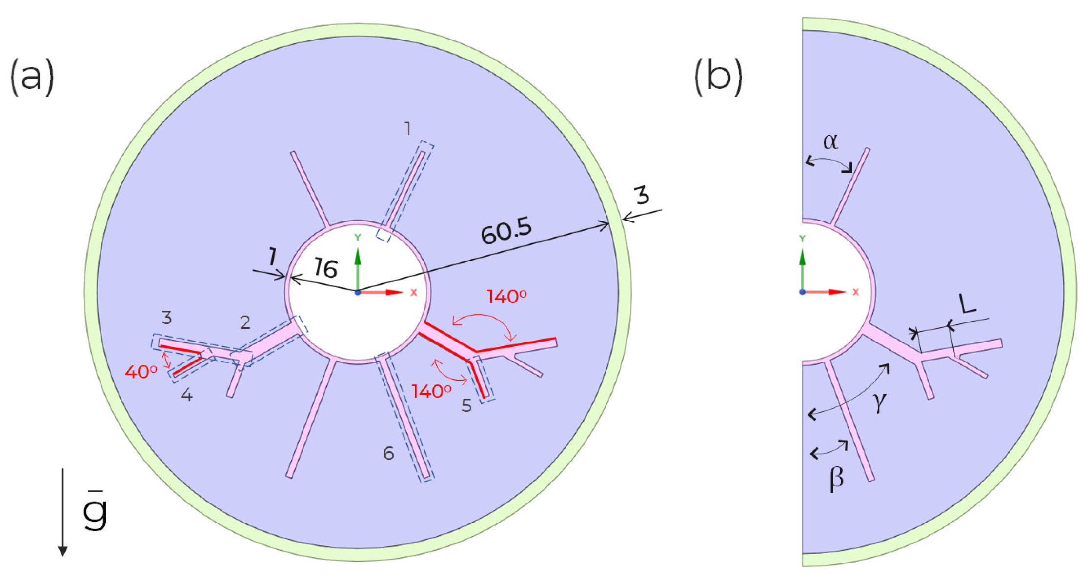
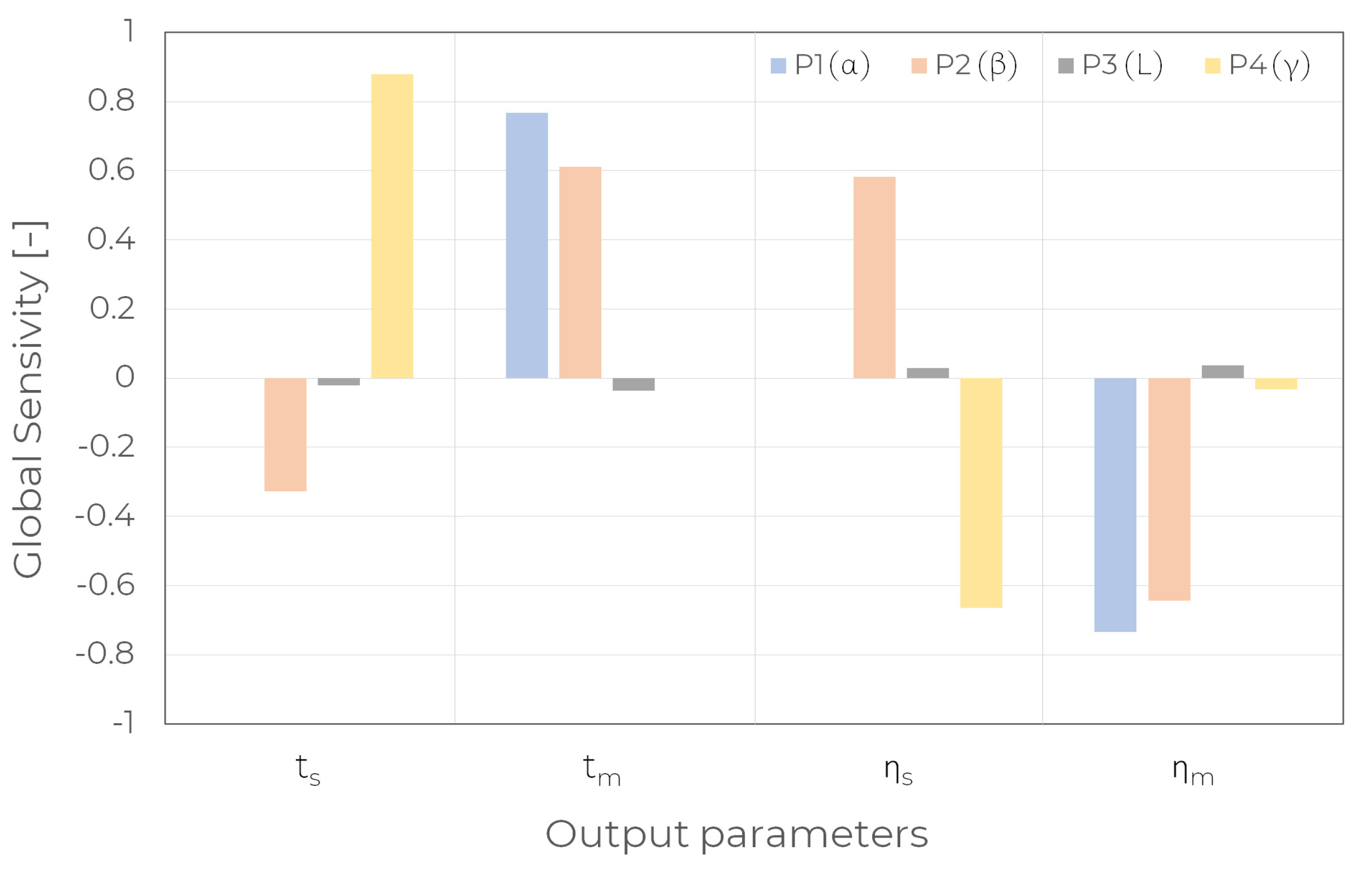
The objective of this research was to identify the global sensitivity analysis (GSA) values and point out the most important geometric parameters of the fin that affect the energy efficiency and phase change times during melting and solidification of the proposed shell-and-tube LHTES unit. For the defined input parameter space, the GSA provides a robust sensitivity measure for the whole space not only at a single point like local sensitivity analysis provides. The GSA also provides the sensitivity values in the presence of both non-linearity and interactions between the parameters [69]. In this research, the GSA for four fin design parameters was used. The analysis of the phase-change interface propagation, PCM temperatures, and velocities was also conducted. This allowed the identification of factors and phenomena affecting the reduction of melting and solidification times. The use of the Design and Analysis of Computer Experiments technique (DACE) allowed identifying the metamodel to quickly assess melting/solidification times and energy efficiency. All these activities are an original element of this research. The multi-objective optimisation is based on the four input parameters: the angle between the top fin and vertical axis, the angle between the lower fin and vertical axis, the length of the fin segment offset and the angle between the tree fin and vertical axis was another objective of this study. The optimisation aimed to maximise the energy efficiency during melting and solidification.

2. LHTES Description and Computational Domain

The three basic components, such as the inner tube, the outer shell, and a PCM-filled space, constitute an LHTES unit. During the charging process, the heat is supplied to the system from the heat transfer fluid (internal side). During discharging, the process occurs in a reverse way. A cross-section of the horizontally oriented shell-and-tube LHTES unit considered in this research is simplified as a two–dimensional annulus. The geometry, presented in Figure 1a, was prepared with reference to the results of a topological optimisation of the fin shape to reduce the melting time [70]. The inner radius of the inner and outer tubes are 16 mm and 60.5 mm, respectively, and the thicknesses are 1 mm and 3 mm, respectively. Each fin, or part of a fin, is marked in Figure 1a with the numbers 1 to 6, and dimensions such as length and width are shown in

Table 1. Dimensions of the individual fins.

Number of Fin	Thickness [mm]	Length [mm]
1	2	20
2	3	14
3	2	20
4	1	10
5	1.5	10
6	1.5	30

. To make a quantitative comparison, the occupied volume of the fins is kept as 2.8% of the whole volume. Half of the cross-section of an LHTES system constitutes the computational domain because of the symmetry of the geometric model, the boundary conditions and the phenomenon taking place. The last condition was investigated by carrying out comparative numerical simulations of the solid-liquid phase change, for the whole section and half of it. The temperature values at selected points are shown in Figure 2. No discrepancies were observed in either the phenomenon or the results analysed. All factors at time strategy were applied and a central composite inscribed (CCI) design was used. Input parameters adopted values on five levels which is the advantage of this type of design. For four factors P1 - P4, there is a need to conduct $2^4+2·4+1=25$ computer experiments. The fins location is designated by four parameters: P1-$\alpha$ denotes the angle between the top fin and y-axis, P2-$\beta$ denotes the angle between the lower fin and y-axis, P3-L is the length of the fin segment offset and P4-$\gamma$ denotes the angle between the tree fin and y-axis. The assumed control variables P1, P2, P3 and P4, shown in Figure 1b, are varied within practically achievable ranges (

Table 2. Input parameters variability range.

Parameter Name	MIN	MAX	Unit
P1	18	28	${}^{°}$
P2	50	90	${}^{°}$
P3	5	12	mm
P4	10	70	${}^{°}$

).

The fin geometrical parameters variability ranges were based on literature data and were proposed by the authors of the study [71,72,73].

3. Methodology

Heat transfer in the LHTES system occurs by natural convection and conduction. Conduction is observed in the tube and fins and the solid-phase PCM. In contrast, heat transfer by convection is dominant at the PCM-pipe interface and in the liquid-phase PCM. An important aspect of the research is to additionally consider solid-liquid and liquid-solid phase change with moving interface.

3.1. Numerical Model Assumptions and Governing Equations

The simulation of solidification/melting and natural convection phenomenon was performed with the following assumptions:

• considered phase change material is RT50 (Rubitherm GmbH),
• the liquid PCM is an incompressible Newtonian fluid,
• the PCM assumed thermophysical values according

  Table 3. Thermophysical properties of PCM (RT50) [74].

  Properties	${\mathit{T}}_{\mathit{s}}$	${\mathit{T}}_{\mathit{l}}$	L	$\mathit{\beta }$	${\mathit{c}}_{\mathit{p}}$	k	${\mathit{\rho }}_{\mathbf{solid}}$	${\mathit{\rho }}_{\mathbf{liquid}}$	$\mathit{\mu }$
  Units	${}^{°}$C	${}^{°}$C	kJ/kg	1/K	J/(kg·K)	W/(m·K)	kg/m3	kg/m3	Pa·s
  PCM	45	51	170.320	0.0006	2000	Figure 3	880 (at 15 ${}^{°}$C)	760 (at 80 ${}^{°}$C)	Figure 3

  ,
• the proper mapping of the PCM thermal conductivity and dynamic viscosity non–linear character reported in [74] the temperature–dependent values from [74] were assumed (Figure 3); as can be seen, thermal conductivity reaches its maximum value near the phase-change temperature, while the dynamic viscosity decreases with the PCM temperature increase,
• the effect of the PCM volumetric expansion, thermal radiative and viscous dissipation are not modelled,
• to take natural convection into account the Boussinesq approximation was used,
• the heat loss to the surrounding was negligible,
• the flow in the liquid phase of the PCM was laminar,
• the temperature change of the pipe wall in space and time has been omitted,
• the third-dimensional heat convection and conduction have been neglected.

Based on the above assumptions the continuity, momentum and energy equations are given below.

The continuity equation including incompressible PCM reduces to the following form:

$$\nabla ·\overrightarrow{v}=0$$

(1)

where v represents the fluid velocity.

In the momentum equation:

$$\frac{\partial \overrightarrow{v}}{\partial t}+\nabla ·\left(\overrightarrow{v}\overrightarrow{v}\right)=\frac{1}{{\rho }_{ref}}(-\nabla p+\mu {\nabla }^2\overrightarrow{v}+\rho \overrightarrow{g})+S\overrightarrow{v}$$

(2)

the Boussinesq approximation was used according to which the fluid density $\rho$ was constant except for the buoyancy term in the momentum equation [75]:

$$\rho ={\rho }_{ref}(1-\beta (T-T_{ref}))$$

(3)

In the above equations, ${\rho }_{ref}$ represents the liquid PCM density at a reference temperature ($T_{ref}=51{}^{°}$C), T denotes the temperature, p stands for the pressure and t represents the time. The symbols $\beta$ and $\mu$ denote thermal expansion coefficient, and dynamic viscosity, respectively and g is the gravitational acceleration ($g=9.81{\mathrm{m}/\mathrm{s}}^2$).

The momentum source term S, according to the enthalpy-porosity approach [76,77], is used to model the mush zone as a porous medium that operates as a partially solidified region. The porosity in each cell signifies the volume of liquid fraction in a cell of a grid system [75]:

$$S=A_{mush}\frac{{(1-\alpha )}^2}{({\alpha }^3+ϵ)}$$

(4)

The mushy zone constant $A_{mush}$ controls the width of the mush zone with a numerical value typically in the range of ${10}^4$–${10}^7$ [78]. In this study, the appropriate value ($3·{10}^6$) of the mushy zone constant is considered considering the finned geometric model [79]. The $\alpha$ represents the liquid fraction, and $ϵ$ is a small number (0.001) added to prevent division by zero.

The thermal energy equation in the PCM domain is as follows:

$${\rho }_{ref}\frac{\partial H}{\partial t}+{\rho }_{ref}\nabla ·\left(\overrightarrow{v}H\right)=\nabla ·(k\nabla T)$$

(5)

H represents the enthalpy, equal to the sum of reference enthalpy $h_{ref}$ at the reference temperature $T_{ref}$, sensible enthalpy and the heat of phase change:

$$H=h_{ref}+{\int }_{T_{ref}}^T{c}_{p}dT+\alpha L$$

(6)

Liquid fraction $\alpha$ can simply be calculated by the dependency in Equation (7):

$$\alpha =\left\{\begin{array}{ccc}0& \mathrm{for}\hfill & T<T_s\hfill \\ 1& \mathrm{for}\hfill & T>T_l\hfill \\ \frac{T-T_s}{T_l-T_s}& \mathrm{for}\hfill & T_s<T<T_l\hfill \end{array}\right.$$

(7)

With decreasing $\alpha$, the velocities decrease, resulting in the porous region becoming a solid. Consequently, the porosity varies from 0 to 1 as the PCM changes from solid to fluid. In the above equations, $c_p$, L, $T_s$, and $T_l$ denote the specific heat capacity, the latent heat, the solid phase temperature and the liquid phase temperature respectively.

3.2. Descriptions of the Initial and Boundary Conditions

To solve the partial differential equations, appropriate boundary and initial conditions must be applied (Equations (1), (2), and (5)). The initial condition of all three subdomains assumes a uniform temperature distribution of 338.15 K for solidification and 313.15 K for melting. The following boundary conditions are assumed:

• the internal wall of the LHTES is assumed to be at a constant temperature of 343.15 K for the melting process and 308.15 K for the solidification process (Figure 4b),
• an adiabatic condition is assumed in the external wall of the unit (Figure 4b),
• a symmetrical boundary condition is considered at the centre–line (Figure 4b),
• the no–slip condition was assumed at the PCM boundary surfaces,
• the ideal contact between the tube and PCM was assumed.

3.3. Numerical Algorithms and Schemes

The ANSYS Fluent 2021R2 simulation environment was used. The simulation was performed using the following algorithms and discretization schemes: to pressure-velocity-coupling, the SIMPLE algorithm was used; to the pressure correction equation, the PRESTO! scheme was used, the convective terms of the momentum and energy equations are discretized using the third-order MUSCL scheme that reduces numerical diffusion and keeps the solution stable; the Least Squares Cell-Based method was used to compute gradients. The convergence criterion was assumed as ${10}^{-5}$ for the continuity equation, ${10}^{-6}$ for the velocity components and ${10}^{-8}$ for the energy equation. The second-order implicit time integration algorithm was selected for the unsteady terms. The assumed time step in the calculations is 0.05 s and the number of iterations for each time step varies between 180 and 300.

3.4. Numerical Model Verification

The independence tests of the present numerical solution were carried out. The unstructured grids (Figure 4a) with a total number of 24,423, 54,159 and 76,979 computational cells, respectively, were used for input parameters $P1={23}^{°}$, $P2={70}^{°}$, $P3=8.5\mathrm{mm}$ and $P4={10}^{°}$. It was ensured that the developed numerical meshes fulfilled the adopted minimum/maximum quality criteria—aspect ratio < 20 and orthogonal quality > 0.4. According to Figure 4c, the total solidification time of the PCM is independent of further increments in grid size above 24,423. Taking the melting process into account, the temperature value at T1 (Figure 2) for all three grids follows a similar trend, with the exception of the moment marked in Figure 4d. These indicate that the grid with 54,159 cells is sufficient for the melting process.

3.5. Numerical Model Validation

The developed numerical model was validated by the experimental work [80]. Kousha et al. [80] performed the experimental study for melting and solidification of RT35 used as a PCM in a shell-and-tube system. Based on the study, the same material data and geometrical parameters were assumed (Figure 5a), and the numerical results we obtained were then compared with the experimental results. During the melting process, an initial water temperature of 80 °C and a flow rate of 0.4 L/min were assumed. The validation results in the form of the mean PCM temperature distribution (Figure 5b) show good agreement with the experimental data. In addition, the average error of the additionally considered temperature curves in individual sections is 5.9%. A similar procedure was adopted to validate the computational model of the solidification process according to the experimental data obtained by Kousha et al. [80]. In the numerical simulation, an initial HTF temperature of 10 ${}^{°}$C was assumed. By analysing the results of both tests, it can be seen that the curves of the average PCM temperature during the first 5000 s have a similar profile. After this time, there are slight deviations in the results, but as the trend of the curves is similar, it is assumed that the numerical model is reliable and can be used for further studies. In addition, it is noted that the average error between the temperature values in individual sections is 4.8%.

4. Discussion of the Simulation Results

The number of computer experiments has been reduced by using the DACE. An extended CCI (central composite inscribed) design was adopted, with factors taking values at five levels. For four factors (P1, P2, P3, P4), 25 numerical experiments were conducted, while in the full-factorial design 625 numerical experiments are required. The output parameters such as ${\eta }_m$ and ${\eta }_s$ are described by two Equations (8) and (9) denote the energy efficiency for melting and solidification process, respectively. The other output parameters are the melting time $t_m$ and the solidification time $t_s$. The simulation was carried out with the use of the supercomputer ‘‘PROMETHEUS’’ in ACK Cyfronet Krakow.

$${\eta }_m=\frac{E_m}{E_{m,max}}$$

(8)

$${\eta }_s=\frac{E_s}{E_{s,max}}$$

(9)

$$E_{m|s,max}=E_{tube,max}+m·[c_p·|T_{peak}-T_{ini|w}|+L+c_p·|T_{w|ini}-T_{peak}\left|\right]+E_{shell,max}$$

(10)

$$E_{tube,max}=m_{tube}·c_{p,tube}·\left[\right|T_w-T_{ini}\left|\right]$$

(11)

$$E_{shell,max}=m_{shell}·c_{p,shell}·\left[\right|T_w-T_{ini}\left|\right]$$

(12)

Table 4. The results of the simulation experiment.

No.	P1-$\mathit{\alpha }$	P2-$\mathit{\beta }$	P3-L	P4-$\mathit{\gamma }$	${\mathit{t}}_{\mathit{m}}$	${\mathit{\eta }}_{\mathit{m}}$	${\mathit{t}}_{\mathit{s}}$	${\mathit{\eta }}_{\mathit{s}}$
	${[}^{°}]$	${[}^{°}]$	[mm]	${[}^{°}]$	[s]	[-]	[s]	[-]
1	20.5	60	6.75	25	6532	0.978	29,272	0.955
2	20.5	60	6.75	55	6498	0.978	38,603	0.938
3	20.5	60	10.25	25	6498	0.978	29,172	0.956
4	20.5	60	10.25	55	6436	0.979	38,490	0.939
5	20.5	80	6.75	25	6988	0.974	25,594	0.979
6	20.5	80	6.75	55	7037	0.973	36,032	0.951
7	20.5	80	10.25	25	6975	0.974	25,456	0.980
8	20.5	80	10.25	55	6948	0.974	35,983	0.951
9	25.5	60	6.75	25	7120	0.973	29,273	0.955
10	25.5	60	6.75	55	7071	0.974	38,601	0.938
11	25.5	60	10.25	25	7088	0.973	29,177	0.956
12	25.5	60	10.25	55	7034	0.974	38,534	0.938
13	25.5	80	6.75	25	7491	0.970	25,557	0.979
14	25.5	80	6.75	55	7498	0.970	36,013	0.951
15	25.5	80	10.25	25	7482	0.970	25,438	0.981
16	25.5	80	10.25	55	7532	0.969	35,968	0.951
17	18	70	8.5	40	6570	0.978	31,233	0.962
18	28	70	8.5	40	7660	0.969	31,167	0.962
19	23	50	8.5	40	6619	0.977	33,669	0.940
20	23	90	8.5	40	7421	0.970	28,197	0.975
21	23	70	5	40	6978	0.974	31,296	0.961
22	23	70	12	40	6933	0.975	31,071	0.963
23	23	70	8.5	10	7008	0.974	28,962	0.960
24	23	70	8.5	70	7033	0.973	43,402	0.925
25	23	70	8.5	40	6958	0.975	31,212	0.962

shows the input values for all 25 design points of the performed simulations and calculated output parameters.

To compare melting and solidification phenomena, the results of numerical simulations in the form of both liquid fraction distributions and velocity and temperature fields in the PCM for four selected LHTES configurations are summarised:

• the configuration with the highest energy efficiency of the melting process (0.979) and the shortest melting time (6463 s)—design point (DP) No. 4,
• the configuration with the highest energy efficiency of the solidification process (0.981) and the shortest solidification time (25,438 s)—DP No. 15,
• the configuration with the lowest energy efficiency of the melting process (0.969) and the longest melting time (7660 s)—DP No. 18,
• the configuration with the lowest energy efficiency of the solidification process (0.925) and the longest solidification time (43,402 s)—DP No. 24.

4.1. Melting Process Analysis

Firstly, the melting processes of PCM with two configurations for 4 and 18 design points are examined to compare the heat transfer characteristics. To illustrate this, the colour maps of the liquid fraction at different times, namely 108 s, 300 s, 1008 s, 2100 s, 3000 s, 10,008 s and 23,400 s are shown in Figure 6. It has been observed that the early stage of the melting process is dominated by heat conduction, which resulted in a thin layer of liquid being formed around the fins due to conductive heat transfer. Over time, the liquid layer becomes larger and non-uniform. It is further noted that the PCM material in the upper region of the domain melts faster, while the phase change of a small layer of it at the bottom takes a significant part of the total melting time. The phase change in both cases occurs in a similar pattern. For design point number 4 in the upper part of the LHTES system, the PCM melts slower, however, it is compensated by a faster phase change in the lower region. As a result, the total melting time for this case is shorter.

Figure 7 compares the temperature distribution for 4 and 18 design points at different time instants. In both cases, a conductive layer appears at the start of melting. After 300 s, the uniform conductive layer destabilises, after which a group of cells is formed that lengthen over time and take the form of plumes. The widening and form of the face affect the curved solid/liquid interface. After 504 s, the cells become larger, causing them to reconnect. Over time, the development of an interface and its movement to the outer wall is observed. A difference in the compared melting processes is the higher temperature of the upper part of the domain in the design point number 18, which can be seen especially after 1008 s. This is due to the placement of the tree fin at a higher angle ($\beta$) than for the 4 DP configuration. However, it is also observed that the temperature between the bottom fins and the bottom and tree fin in case number 4 is higher than for the 18 DP configuration, leading to an earlier achievement of the phase change temperature and accelerated melting in this area. The larger area of the lower LHTES part covered by the phase change temperature is associated with the placement of the bottom fin at a lower angle than for the 18 DP.

Figure 8 shows the velocity profiles of PCM for two configurations of finned tube LHTES systems. At the initial stages of the melting process, the thin liquid film forms all over the inner tube and the fins. In both cases, small circulation vortices are then generated at the top of the inner pipe and above the tree fin. Simultaneously along the lower fin, there is an expansion of the conductive layer. After the convection cells in the upper part of the system are connected, they dynamically grow and change shape. The temperature difference between the area around the fins and the rest of the liquid translates into a difference in the density of the liquid and causes buoyancy forces. As a result, natural convection becomes the dominant heat transfer mechanism at the top of the system and results in a moving solid/liquid interface. Up to the 300th second of the phase change, the velocity distribution looks similar. At 504 s, the velocity and size of the vortices flowing around the upper fin are higher for case number 18. At the next moment, also for this case, larger and denser vortices are observed in the upper domain. However, at 2004 and 3000 s, the heat transfer process by natural convection is more intense for case number 4. At the end of the melting, a dominance of heat conduction is observed. A significant influence on the reduction of melting time is the placement of the bottom fin at a lower angle, as can be seen in Figure 8a. This fin act as an obstacle, preventing the melting front from going up. Despite the delay in melting at the top of the domain, this helps reinforce the conduction in the bottom part. Furthermore, placing the top fin at a higher angle, although it delays the heating of the upper domain (Figure 7), facilitates the movement of convection currents in the second part of the melting process. It is further noted that the angle of placement of the tree fin has no significant effect on the process.

4.2. Solidification Process Analysis

The solidification process at different times, namely 108 s, 300 s, 1008 s, 2100 s, 3000 s, 10,008 s and 23,400 s, has also been considered. Figure 9 shows the evolution of the solid fraction distribution. During the initial stage of solidification, the solid phase of the PCM continuously expanded with the geometry of the fin. As time passed, the thickness of this layer increased, which contributed to weakening the direct heat transfer between the high-conductivity fins and the PCM. This causes the solidification process to slow down after 3000 s. The most significant influence on the reduction of the phase change time is the placement of the top fin. Using a smaller angle of inclination, as in design point number 15, results in the solid/liquid interface moving faster upwards. For the initial 3000 s, the volume of solid PCM is approximately similar, but a larger amount is present in the upper region of the domain. It is noted that the PCM material then solidifies at the bottom of the LHTES system, at a faster rate for design point number 15. Subsequently, the phase change of the liquid PCM occurs in the upper part of the domain, which takes a considerable amount of time. As a result, a smaller amount of solidified material is observed for design point number 24.

Figure 10 depicts the time-wise variation of the temperature of PCM. Initially, the area around the fins is cooled to the temperature of the phase change. What is more, in both cases considered, there is a temperature drop of about 7 K in the bottom part of the domain in the first 108 s of the process. Also significant seems to be the appearance of small ribbon-shaped areas, with even lower temperatures, within the tree and lower fin, suggesting the formation of convection cells. Initially, the phase change temperature is reached by the lower part of the domain, followed by the upper part—but at a much slower rate. Cooling and phase change of the liquid PCM is the fastest for design point number 15. As the top fins are placed at a lower angle than for design point 24, a faster temperature drop occurs in the area between them. In addition, there is a larger area of lower temperature between the top fin and the tree fin.

Figure 11 presents colour maps of the velocity of the solidifying PCM. In the first 660 s, the formation of convection cells in the lower part is observed. It was noted earlier that the greatest temperature difference between the areas of liquid PCM with high temperature and the solidified material near the fins is at the beginning of the process. Therefore, convection cells form below the fins and their velocity decreases with time. After 1008 s, the temperature gradient at the bottom of the domain is much smaller, hence natural convection has less influence in the solidification process. In the 3000th s, natural convection has less influence on the heat transfer in the system, due to the disappearance of convection cells. Instead, conduction starts to dominate in the upper part of the domain, and the velocity of movement of the solid/liquid interface is low compared to the beginning of the process. In design point number 15, placing the top fin at the lowest angle value results in the appearance of larger convection cells between the top fin and the tree fin. Therefore, intensive heat exchange occurs over a larger area than in design point number 24. Furthermore, the convection cell under the top fin drives another circulation cell that forms between the axis of symmetry and the top fin, which accelerates heat exchange in this area during the early stages of the process.

The computational model, despite describing the melting/solidification process with considerable accuracy, does not take into account several hidden phenomena: (i) heat loss to the surroundings on the outer wall was ignored; (ii) changes in the volume of the PCM during the phase change were not taken into account; (iii) the existence of thermal resistance between materials in the solid phase was neglected; (iv) perfect concentricity was assumed in the geometrical model; (v) the temperature change along the HTF pipe length was ignored. It is worth highlighting that in practical implementation, these phenomena affect the melting and solidification process.

4.3. The Multidimensional Response Surface

The DACE with the central composite inscribed design needed the additional design points, the so-called refinement points. This strategy with the use of sophisticated approximation algorithms allows the multidimensional response surface to be developed with good quality. The twelve refinement simulation experiments and all design points were approximated using the Genetic Aggregation algorithm based on Ansys implementation [75]. The complex multidimensional function $y_{\widehat{m}}\left(x_{1-4}\right)$ with numerous coefficients is presented in implicit form as the file with the extension .dxrom, which can then be used in Matlab or Excel software.

$$y_{\widehat{m}}\left(x_{1-4}\right)=\sum _{i=1}^{N_m}{w}_i{y}_{\widehat{m},i}\left(x_{1-4}\right)$$

(13)

where, $y_{\widehat{m},i}\left(x_{1-4}\right)$—is the prediction of the i-th meta-model, $N_m$—is the number of meta-models used, $w_i$—is the weight factor of the i-th meta-model, which satisfies ${\sum }_{i=1}^N{w}_i=1$. As a result, it is possible to qualitatively assess the influence of the design parameters of the LHTES on melting, solidification times and energy efficiency. The three step verification of metamodel (Equation (13)) was done. The first was dedicated to evaluating the compatibility of the metamodel with the physics of the phenomenon. The second was to calculate and evaluate the values of the root mean square error (RMSE) and the determination coefficient $R^2$ values. The third was to calculate the RMSE (Figure 12) at five randomly selected points.

In Figure 13 the multidimensional response surface was obtained from the design parameters P1, P2 and the output parameters $t_m$, $t_s$, ${\eta }_m$, ${\eta }_s$. The response surface depends on two more design parameters, P3 = 〈6.75 mm; 10.25 mm〉 and P4 = 〈25${}^{°}$; 55${}^{°}$〉. The melting time $t_m$, varies between 6436 s for DP No. 4 to 7660 s for DP No. 18. In the case of energy efficiency of the melting process ${\eta }_m$, the values vary in the range of 0.969 for DP No. 18 to 0.979 for DP No. 4. The solidification time $t_s$, varies between 25,438 s for DP No. 15 to 43,402 s for DP No. 24. In the case of energy efficiency of the solidification process ${\eta }_s$, the values vary in the range of 0.925 for DP No. 24 to 0.981 for DP No. 15. As the parameters P1 ($\alpha$) and P2 ($\beta$) decrease, the melting time $t_m$ decreases, reaching the lowest value in the adopted range (Table 2). The energy efficiency of the melting process ${\eta }_m$, on the other hand, improves with increasing P1 and P2. The solidification time $t_s$ decreases with parameter P4, as can be seen from the arrangement of the four response surfaces. The value $t_s$ decreases with the increase in the value of P2, and for smaller values of P4, this behaviour is pronounced. It is observed that the relationship between the solidification time and energy efficiency of the solidification process is inversely proportional. Therefore, an increase in the value of the P2 and a decrease in P4 results in an increase in the energy efficiency value of ${\eta }_s$. It is also noticed that the parameter P3 has a minor effect on the determined output parameters.

In Figure 14 the multidimensional response surface was obtained from the design parameters P3, P4 and the output parameters $t_m$, $t_s$, ${\eta }_m$, ${\eta }_s$. The response surface depends on two more design parameters, P1 = 〈20.5${}^{°}$; 25.5${}^{°}$〉 and P2 = 〈60${}^{°}$; 80${}^{°}$〉. As the parameter P4 increases, the melting time initially decreases, reaching a minimum, and then increases again. The shortest melting times are noted at P4 ≈ 40${}^{°}$ (for parameter P2 = 80${}^{°}$) and at P4 ≈ 55${}^{°}$ (for parameter P2 = 60${}^{°}$). Furthermore, a decrease in the value of the P3 is associated with an increase in the melting time. The effect of the P3 parameter on the energy efficiency of the melting process, on the other hand, is the opposite - with an increase in the P3 parameter, the energy efficiency increases. It should be noted that the effects of both parameters analysed on $t_m$ and ${\eta }_m$ are negligible. The solidification time initially decreases with increasing parameter P4, reaching a minimum at P4 ≈ 25${}^{°}$ for P2 = 60${}^{°}$ and at P4 ≈ 20${}^{°}$ for P2 = 80${}^{°}$. An inverse relationship is observed for the energy efficiency of the solidification process. The influence of parameter P3 on $t_m$ and ${\eta }_s$ is minor.

In Figure 15 the multidimensional response surface was obtained from the design parameters P2, P4 and the output parameters $t_m$, $t_s$, ${\eta }_m$, ${\eta }_s$. The response surface depends on two more design parameters, P1 = 〈20.5${}^{°}$; 25.5${}^{°}$〉 and P3 = 〈6.75 mm; 10.25 mm〉. As mentioned above, the P2 parameter, i.e., tree fin angle has an impact on the melting and solidification times and the energy efficiency during melting and solidification. As this parameter increases, the melting time improves, while reducing the energy efficiency of the melting process. However, by increasing P2, solidification time is reduced and energy efficiency is improved. When the value of another parameter is changed, the behaviour of the given relationship remains the same. As the angle of the top fin, described by the parameter P4, increases, the melting time decreases and the energy efficiency of the process improves, but the differences in the achieved output values are practically unnoticeable. An increase in P4 results in an initial shortening and then lengthening of the solidification time—i.e., analogously an increase and a decrease in the energy efficiency during solidification. As the P2 parameter increases, this change is more noticeable. Changes in P1 and P3 parameters only have a significant effect on the melting process. With the decrease in these parameters, melting time is reduced and energy efficiency is improved. The angle of the bottom fin (parameter P1), has a significantly greater influence on the course of the melting process than the length of the fin segment offset (parameter P4). However, compared to the P2 parameter, the P1 parameter is less important. With the increase in the P3 parameter, the melting time decreases slightly and the energy efficiency value increases.

4.4. Global Sensitivity Analysis

The authors used correlation coefficients as a measure of sensitivity and calculated it from the scatter plots of the output variables in relation to the individual design variables, after sampling the metamodel over its input distributions.

The correlation between the two variables identified as $x_i$ and $y_i$, for n = 4000 randomly selected pairs of points {($x_i$, $y_i$), … , ($x_n$, $y_n$)}, and where x and y are the mean values of $\widehat{x}$ and $\widehat{y}$ respectively, can be written as:

$$r_{xy}=\frac{{\sum }_{i=1}^n\left(x_i-\widehat{x}\right)\left(y_i-\widehat{y}\right)}{\sqrt{{\sum }_{i=1}^n{\left(x_i-\widehat{x}\right)}^2{\sum }_{i=1}^n{\left(y_i-\widehat{y}\right)}^2}}$$

(14)

Figure 16 presents the sensitivities calculated by the correlation coefficient method. It is noticed that the evident influence on the solidification time has the angles of the top and tree fins (parameters P2 and P4) and as their values increase, the solidification time decrease and increase, respectively. When considering the energy efficiency of solidification, an increase in the angle of inclination of the tree fin has a positive effect. Increasing the value of the top fin angle leads to a decrease in energy efficiency ${\eta }_s$. As noted previously, the parameter P1, the angle of the bottom fin, is more significant in the melting process compared to the parameter P2 (the angle of the tree fin). However, as the values of these parameters increase, the melting time increase, leading to a decrease in energy efficiency ${\eta }_m$. It was noticed that parameter P3 has no significant effect on all output parameters.

4.5. Multi-Objective Optimisation

A multi-objective optimisation was further performed to maximise energy efficiency during melting and solidification $max\left({\eta }_m,{\eta }_s\right)$. The multi-objective function (Equation (15)) is presented as follows:

$$\mathsf{\Phi }=\sum _{j=1}^m{w}_j{M}_j$$

(15)

where m—is the number of output parameters, $\mathsf{\Phi }$—is the objective function, $w_j$—are the individual weights $(w_s>w_m)$, $M_j$—is the single weighted objective function.

Scalable partial objectives are defined as (Equation (16)):

$$M_j={\left(\frac{\left|{y^{*}}_t-y\right|}{y_{max}-y_{min}}\right)}_j$$

(16)

where ${y^{*}}_t$—are the j-th intended values of the output parameters in the system (for example minimal, maximal), y—are the values obtained based on the meta-model for quantities ${\eta }_m$ and ${\eta }_s$ and $y_{min}$, $y_{max}$ respectively: the maximum and minimum y value.

The range of input variables is described in Table 2. To estimate the parameters the concept of Pareto dominance on the predicted response surface was used. To perform the optimisation process, a screening algorithm was used. It was assumed that it was more important to improve the energy efficiency of the solidification process, due to its much larger range of values. As part of the configuration of the optimisation process, 4000 samples were generated, and three candidate points were found. In Figure 17 the trade-off chart for design parameters was presented.

Based on this relationship, Pareto-dominant solutions were observed and a candidate point was determined for which the highest possible ${\eta }_s$ value is reached for the highest ${\eta }_m$ value. This point coincides with the solution obtained by the screening method (

Table 5. Candidate points determined by the screening method.

Name	P1	P2	P3	P4	${\mathit{\eta }}_{\mathit{m}}$	${\mathit{\eta }}_{\mathit{s}}$
Candidate Point 1	18.2	89.0	10.7	21.0	0.973	0.988
Candidate Point 2	21.8	89.9	11.1	15.5	0.971	0.989
Candidate Point 3	27.4	89.6	8.8	10.5	0.965	0.987

) and has been labelled ‘Candidate Point 1’.

After selecting the optimal candidate point, the energy efficiency of the solidification and melting processes was verified.

Table 6. Verification of optimisation results.

Name	${\mathit{\eta }}_{\mathit{m}}$	${\mathit{\eta }}_{\mathit{s}}$	Relative Error for ${\mathit{\eta }}_{\mathit{m}}$ [%]	Relative Error for ${\mathit{\eta }}_{\mathit{s}}$ [%]	${\mathit{t}}_{\mathit{m}}$	${\mathit{t}}_{\mathit{s}}$	Relative Error for ${\mathit{t}}_{\mathit{m}}$ [%]	Relative Error for ${\mathit{t}}_{\mathit{s}}$ [%]
RSM result	0.9727	0.9884	0.02	0.20	7086	23,502	0.11	0.54
Calculation result	0.9725	0.9865	0.02	0.20	7094	23,628	0.11	0.54

shows a comparison between the results of the numerical simulation carried out for the optimum geometric parameters (Table 5) and the results taken from the response surface. The discrepancy is 0.02% for ${\eta }_m$ and 0.2% for ${\eta }_s$.

5. Conclusions

The authors investigate the influence of four geometric parameters ($\alpha$, $\beta$, $\gamma$ angles and fin segment offset L) on melting time, solidification time and energy efficiency during that processes. For this purpose, an extended CCI design was adopted and a multidimensional response surface was designed using Genetic Aggregation. After a response surface was determined, global sensitivity analysis and multi-objective optimisation were performed to estimate the influence parameters and maximise the energy efficiency of the melting and solidification process. Furthermore, for the cases with the longest and shortest melting and solidification times (corresponding to the highest and lowest energy efficiencies), the phase change processes were compared based on the distribution of liquid fraction, temperature and velocity. The most important conclusions could be summarised below:

• The solidification time and process efficiency are strongly sensitive to the top fin angle (P4-$\gamma$) and the position of the tree fin (P2-$\beta$) variation.
• The melting time and process efficiency are strongly sensitive to the angle of the bottom fin (P1-$\alpha$) and the position of the tree fin (P2-$\beta$) variation.
• Decreasing the angle of the bottom fin (P1-$\alpha$) reduces the melting time and increases the energy efficiency during this process.
• The position of the tree fin (P2-$\beta$ angle) has an unclear effect on the melting and solidification time.
• Changing the value of the top fin angle (P4-$\gamma$) does not significantly affect the melting process. However, by decreasing the value of this angle, the solidification time decreases and the energy efficiency during this process increases.
• The use of global sensitivity analysis to determine the effect of geometric parameters on the energy efficiency of phase change can lead to the design of efficient LHTES units, for example in solar thermal collector systems.
• When analysing the response plots (Figure 14 and Figure 15), however, it is found that $\gamma$ angle values below 25${}^{°}$ can result in longer solidification times and worsen energy efficiency. However, as the angle of the tree fin increases, this effect is less pronounced.
• As part of a multi-objective optimisation to increase the energy efficiency of the melting and solidification process, the optimum fin arrangement in the LHTES was obtained. The following geometrical parameter values were adopted: $\alpha =18.2^{°}$, $\beta =89.0^{°}$, $L=10.7$ mm and $\gamma =21.0^{°}$. The efficiencies of the optimised system during melting and solidification are ${\eta }_m=0.9725\%$ and ${\eta }_s=0.9865\%$. The phase change times reach $t_m=7094$ s and $t_s=$ 23,628 s. The obtained values are a compromise solution, aiming to achieve the highest possible efficiency values for both melting and solidification processes.

Thus, to properly analyse the PCM phase change process in LHTES, additional experiments would have to be performed in a unit with optimised geometrical parameters. It will be valuable to develop a further geometrical model based on the optimum placement of the fins, particularly to significantly reduce the melting time. As a further direction of the study, the authors also propose to analyse the influence of the operating parameters and to obtain the exergy efficiency of the LHTES.

References

1. Paul, A.; Holy, F.; Textor, M.; Lechner, S. High temperature sensible thermal energy storage as a crucial element of Carnot Batteries: Overall classification and technical review based on parameters and key figures. J. Energy Storage 2022, 56, 106015. [Google Scholar] [CrossRef]
2. Opolot, M.; Zhao, C.; Liu, M.; Mancin, S.; Bruno, F.; Hooman, K. A review of high temperature (≥500 °C) latent heat thermal energy storage. Renew. Sustain. Energy Rev. 2022, 160, 112293. [Google Scholar] [CrossRef]
3. Hu, N.; Li, Z.R.; Xu, Z.W.; Fan, L.W. Rapid charging for latent heat thermal energy storage: A state-of-the-art review of close-contact melting. Renew. Sustain. Energy Rev. 2022, 155, 111918. [Google Scholar] [CrossRef]
4. Li, G.; Hwang, Y.; Radermacher, R. Experimental investigation on energy and exergy performance of adsorption cold storage for space cooling application. Int. J. Refrig. 2014, 44, 23–35. [Google Scholar] [CrossRef]
5. Khadiran, T.; Hussein, M.Z.; Zainal, Z.; Rusli, R. Advanced energy storage materials for building applications and their thermal performance characterization: A review. Renew. Sustain. Energy Rev. 2016, 57, 916–928. [Google Scholar] [CrossRef]
6. Jaguemont, J.; Omar, N.; den Bossche, P.V.; Mierlo, J. Phase-change materials (PCM) for automotive applications: A review. Appl. Therm. Eng. 2018, 132, 308–320. [Google Scholar] [CrossRef]
7. Hassan, F.; Jamil, F.; Hussain, A.; Ali, H.M.; Janjua, M.M.; Khushnood, S.; Farhan, M.; Altaf, K.; Said, Z.; Li, C. Recent advancements in latent heat phase change materials and their applications for thermal energy storage and buildings: A state of the art review. Sustain. Energy Technol. Assess. 2022, 49, 101646. [Google Scholar] [CrossRef]
8. Li, Q.; Li, C.; Du, Z.; Jiang, F.; Ding, Y. A review of performance investigation and enhancement of shell and tube thermal energy storage device containing molten salt based phase change materials for medium and high temperature applications. Appl. Energy 2019, 255, 113806. [Google Scholar] [CrossRef]
9. Tao, Y.B.; He, Y.L. A review of phase change material and performance enhancement method for latent heat storage system. Renew. Sustain. Energy Rev. 2018, 93, 245–259. [Google Scholar] [CrossRef]
10. Rathore, P.K.S.; Shukla, S.K. Enhanced thermophysical properties of organic PCM through shape stabilization for thermal energy storage in buildings: A state of the art review. Energy Build. 2021, 236, 110799. [Google Scholar] [CrossRef]
11. Liu, M.; Saman, W.; Bruno, F. Review on storage materials and thermal performance enhancement techniques for high temperature phase change thermal storage systems. Renew. Sustain. Energy Rev. 2012, 16, 2118–2132. [Google Scholar] [CrossRef]
12. Lin, X.; Chen, X.; Weng, L.; Hu, D.; Qiu, C.; Liu, P.; Zhang, Y.; Fan, M.; Sun, W.; Guo, X. In-situ copper ion reduction and micro encapsulation of wood-based composite PCM with effective anisotropic thermal conductivity and energy storage. Sol. Energy Mater. Sol. Cells 2022, 242, 111762. [Google Scholar] [CrossRef]
13. Mostafavi, A.; Jain, A. Thermal Management Effectiveness and Efficiency of a Fin Surrounded by a Phase Change Material (PCM). Int. J. Heat Mass Transf. 2022, 191, 122630. [Google Scholar] [CrossRef]
14. Shen, Y.; Mazhar, A.R.; Liu, S. Comprehensive review on cascaded latent heat storage technology: Recent advances and challenges. J. Energy Storage 2022, 55, 105713. [Google Scholar] [CrossRef]
15. Aurangzeb, M.; Noor, F.; Qamar, A.; Shah, A.N.; Kumam, P.; Shah, Z.; Shutaywi, M. Investigation of enhancement in the thermal response of phase change materials through nano powders. Case Stud. Therm. Eng. 2022, 29, 101654. [Google Scholar] [CrossRef]
16. Zahid, I.; Farooq, M.; Farhan, M.; Usman, M.; Qamar, A.; Imran, M.; Alqahtani, M.A.; Anwar, S.; Sultan, M.; Javaid, M.Y. Thermal Performance Analysis of Various Heat Sinks Based on Alumina NePCM for Passive Cooling of Electronic Components: An Experimental Study. Energies 2022, 15, 8416. [Google Scholar] [CrossRef]
17. Meng, Z.N.; Zhang, P. Experimental and numerical investigation of a tube-in-tank latent thermal energy storage unit using composite PCM. Appl. Energy 2017, 190, 524–539. [Google Scholar] [CrossRef]
18. Deng, Y.; Li, J.; Qian, T.; Guan, W.; Li, Y.; Yin, X. Thermal conductivity enhancement of polyethylene glycol/expanded vermiculite shape-stabilized composite phase change materials with silver nanowire for thermal energy storage. Chem. Eng. J. 2016, 295, 427–435. [Google Scholar] [CrossRef]
19. Cui, W.; Yuan, Y.; Sun, L.; Cao, X.; Yang, X. Experimental studies on the supercooling and melting/freezing characteristics of nano-copper/sodium acetate trihydrate composite phase change materials. Renew. Energy 2016, 99, 1029–1037. [Google Scholar] [CrossRef]
20. Şahan, N.; Fois, M.; Paksoy, H. Improving thermal conductivity phase change materials—A study of paraffin nanomagnetite composites. Sol. Energy Mater. Sol. Cells 2015, 137, 61–67. [Google Scholar] [CrossRef]
21. Xiao, X.; Zhang, P.; Li, M. Preparation and thermal characterization of paraffin/metal foam composite phase change material. Appl. Energy 2013, 112, 1357–1366. [Google Scholar] [CrossRef]
22. Lin, Y.; Jia, Y.; Alva, G.; Fang, G. Review on thermal conductivity enhancement, thermal properties and applications of phase change materials in thermal energy storage. Renew. Sustain. Energy Rev. 2018, 82, 2730–2742. [Google Scholar] [CrossRef]
23. Huang, Y.; Liu, X. Charging and discharging enhancement of a vertical latent heat storage unit by fractal tree-shaped fins. Renew. Energy 2021, 174, 199–217. [Google Scholar] [CrossRef]
24. Du, J.; Ren, F.; Cai, Y.; Shi, D.; Zheng, S.; Chu, X.; Yu, X. Thermal performance analysis of triple casing latent heat system based on sinusoidal function type corrugation. Case Stud. Therm. Eng. 2022, 36, 102168. [Google Scholar] [CrossRef]
25. Pan, C.; Vermaak, N.; Wang, X.; Romero, C.; Neti, S.; Chen, C.H.; Bonner, R. A fast dynamic model for a large scale heat pipe embedded latent heat thermal energy storage system for optimal sizing and control. J. Energy Storage 2022, 51, 104489. [Google Scholar] [CrossRef]
26. Mahdavi, A.; Moghaddam, M.A.E.; Mahmoudi, A. Simultaneous charging and discharging of multi-tube heat storage systems using copper fins and Cu nanoparticles. Case Stud. Therm. Eng. 2021, 27, 101343. [Google Scholar] [CrossRef]
27. Kumar, A.; Saha, S.K. Thermal and structural characterizations of packed bed thermal energy storage with cylindrical micro-encapsulated phase change materials. J. Energy Storage 2022, 48, 103948. [Google Scholar] [CrossRef]
28. Cao, Y.; Ayed, H.; Algelany, A.M.; Dahari, M.; Nguyen, P.Q.P.; Gepreel, K.A.; Nguyen, V.N.; Ehab, M.; Wae-Hayee, M. Receiving heat from a PCM tank by using natural convection of water and NEPCM: A simulation for LHTES application. Case Stud. Therm. Eng. 2022, 35, 102123. [Google Scholar] [CrossRef]
29. Seddegh, S.; Wang, X.; Henderson, A.D. A comparative study of thermal behaviour of a horizontal and vertical shell-and-tube energy storage using phase change materials. Appl. Therm. Eng. 2016, 93, 348–358. [Google Scholar] [CrossRef]
30. Cao, X.; Yuan, Y.; Xiang, B.; Sun, L.; Xingxing, Z. Numerical investigation on optimal number of longitudinal fins in horizontal annular phase change unit at different wall temperatures. Energy Build. 2018, 158, 384–392. [Google Scholar] [CrossRef]
31. Tao, Y.B.; He, Y.L. Effects of natural convection on latent heat storage performance of salt in a horizontal concentric tube. Appl. Energy 2015, 143, 38–46. [Google Scholar] [CrossRef]
32. Wołoszyn, J.; Szopa, K.; Czerwiński, G. Enhanced heat transfer in a PCM shell-and-tube thermal energy storage system. Appl. Therm. Eng. 2021, 196, 117332. [Google Scholar] [CrossRef]
33. Deng, S.; Nie, C.; Wei, G.; Ye, W.B. Improving the melting performance of a horizontal shell-tube latent-heat thermal energy storage unit using local enhanced finned tube. Energy Build. 2019, 183, 161–173. [Google Scholar] [CrossRef]
34. Zhao, C.; Opolot, M.; Liu, M.; Bruno, F.; Mancin, S.; Hooman, K. Numerical study of melting performance enhancement for PCM in an annular enclosure with internal-external fins and metal foams. Int. J. Heat Mass Transf. 2020, 150, 119348. [Google Scholar] [CrossRef]
35. Khan, L.A.; Khan, M.M. Role of orientation of fins in performance enhancement of a latent thermal energy storage unit. Appl. Therm. Eng. 2020, 175, 115408. [Google Scholar] [CrossRef]
36. Yang, X.; Wang, X.; Liu, Z.; Luo, X.; Yan, J. Effect of fin number on the melting phase change in a horizontal finned shell-and-tube thermal energy storage unit. Sol. Energy Mater. Sol. Cells 2022, 236, 111527. [Google Scholar] [CrossRef]
37. Nie, C.; Deng, S.; Liu, J. Effects of fins arrangement and parameters on the consecutive melting and solidification of PCM in a latent heat storage unit. J. Energy Storage 2020, 29, 101319. [Google Scholar] [CrossRef]
38. Ji, C.; Qin, Z.; Dubey, S.; Choo, F.H.; Duan, F. Simulation on PCM melting enhancement with double-fin length arrangements in a rectangular enclosure induced by natural convection. Int. J. Heat Mass Transf. 2018, 127, 255–265. [Google Scholar] [CrossRef]
39. Li, H.; Hu, C.; He, Y.; Tang, D.; Wang, K. Influence of fin parameters on the melting behavior in a horizontal shell-and-tube latent heat storage unit with longitudinal fins. J. Energy Storage 2021, 34, 102230. [Google Scholar] [CrossRef]
40. Yu, C.; Zhang, X.; Chen, X.; Zhang, C.; Chen, Y. Melting performance enhancement of a latent heat storage unit using gradient fins. Int. J. Heat Mass Transf. 2020, 150, 119330. [Google Scholar] [CrossRef]
41. Nobrega, C.R.; Ismail, K.A.; Lino, F.A. Solidification around axial finned tube submersed in PCM: Modeling and experiments. J. Energy Storage 2020, 29, 101438. [Google Scholar] [CrossRef]
42. Shahsavar, A.; Goodarzi, A.; Mohammed, H.I.; Shirneshan, A.; Talebizadehsardari, P. Thermal performance evaluation of non-uniform fin array in a finned double-pipe latent heat storage system. Energy 2020, 193, 116800. [Google Scholar] [CrossRef]
43. Li, Z.; Wu, Z.G. Analysis of HTFs, PCMs and fins effects on the thermal performance of shell–tube thermal energy storage units. Sol. Energy 2015, 122, 382–395. [Google Scholar] [CrossRef]
44. Joybari, M.M.; Haghighat, F.; Seddegh, S.; Al-Abidi, A.A. Heat transfer enhancement of phase change materials by fins under simultaneous charging and discharging. Energy Convers. Manag. 2017, 152, 136–156. [Google Scholar] [CrossRef]
45. Abdulateef, A.M.; Mat, S.; Sopian, K.; Abdulateef, J.; Gitan, A.A. Experimental and computational study of melting phase-change material in a triplex tube heat exchanger with longitudinal/triangular fins. Sol. Energy 2017, 155, 142–153. [Google Scholar] [CrossRef]
46. Aly, K.A.; El-Lathy, A.R.; Fouad, M.A. Enhancement of solidification rate of latent heat thermal energy storage using corrugated fins. J. Energy Storage 2019, 24, 100785. [Google Scholar] [CrossRef]
47. Lohrasbi, S.; Bandpy, M.G.; Ganji, D.D. Response surface method optimization of V-shaped fin assisted latent heat thermal energy storage system during discharging process. Alex. Eng. J. 2016, 55, 2065–2076. [Google Scholar] [CrossRef] [Green Version]
48. Ahmad, W.; Syed, K.S.; Ishaq, M.; Hassan, A.; Iqbal, Z. Numerical study of conjugate heat transfer in a double-pipe with exponential fins using DGFEM. Appl. Therm. Eng. 2017, 111, 1184–1201. [Google Scholar] [CrossRef]
49. Wu, L.; Zhang, X.; Liu, X. Numerical analysis and improvement of the thermal performance in a latent heat thermal energy storage device with spiderweb-like fins. J. Energy Storage 2020, 32, 101768. [Google Scholar] [CrossRef]
50. Sheikholeslami, M.; Lohrasbi, S.; Ganji, D.D. Numerical analysis of discharging process acceleration in LHTESS by immersing innovative fin configuration using finite element method. Appl. Therm. Eng. 2016, 107, 154–166. [Google Scholar] [CrossRef]
51. Scharinger-Urschitz, G.; Walter, H.; Haider, M. Heat Transfer in Latent High-Temperature Thermal Energy Storage Systems—Experimental Investigation. Energies 2019, 12, 1264. [Google Scholar] [CrossRef] [Green Version]
52. Keshteli, A.N.; Sheikholeslami, M. Influence of Al2O3 nanoparticle and Y-shaped fins on melting and solidification of paraffin. J. Mol. Liq. 2020, 314, 113798. [Google Scholar] [CrossRef]
53. Liu, S.; Peng, H.; Hu, Z.; Ling, X.; Huang, J. Solidification performance of a latent heat storage unit with innovative longitudinal triangular fins. Int. J. Heat Mass Transf. 2019, 138, 667–676. [Google Scholar] [CrossRef]
54. Ma, J.; Xu, H.; Liu, S.; Peng, H.; Ling, X. Numerical study on solidification behavior and exergy analysis of a latent heat storage unit with innovative circular superimposed longitudinal fins. Int. J. Heat Mass Transf. 2021, 169, 120949. [Google Scholar] [CrossRef]
55. Sarani, I.; Payan, S.; Nada, S.A.; Payan, A. Numerical investigation of an innovative discontinuous distribution of fins for solidification rate enhancement in PCM with and without nanoparticles. Appl. Therm. Eng. 2020, 176, 115017. [Google Scholar] [CrossRef]
56. Al-Mudhafar, A.H.; Nowakowski, A.F.; Nicolleau, F.C. Enhancing the thermal performance of PCM in a shell and tube latent heat energy storage system by utilizing innovative fins. Energy Rep. 2021, 7, 120–126. [Google Scholar] [CrossRef]
57. Pahamli, Y.; Hosseini, M.J.; Ardahaie, S.S.; Ranjbar, A.A. Improvement of a phase change heat storage system by Blossom-Shaped Fins: Energy analysis. Renew. Energy 2022, 182, 192–215. [Google Scholar] [CrossRef]
58. Kamkari, B.; Shokouhmand, H.; Bruno, F. Experimental investigation of the effect of inclination angle on convection-driven melting of phase change material in a rectangular enclosure. Int. J. Heat Mass Transf. 2014, 72, 186–200. [Google Scholar] [CrossRef]
59. Huang, R.; Mahvi, A.; Odukomaiya, W.; Goyal, A.; Woods, J. Reduced-order modeling method for phase-change thermal energy storage heat exchangers. Energy Convers. Manag. 2022, 263, 115692. [Google Scholar] [CrossRef]
60. Hosseinzadeh, K.; Alizadeh, M.; Tavakoli, M.H.; Ganji, D.D. Investigation of phase change material solidification process in a LHTESS in the presence of fins with variable thickness and hybrid nanoparticles. Appl. Therm. Eng. 2019, 152, 706–717. [Google Scholar] [CrossRef]
61. Gürtürk, M.; Kok, B. A new approach in the design of heat transfer fin for melting and solidification of PCM. Int. J. Heat Mass Transf. 2020, 153, 119671. [Google Scholar] [CrossRef]
62. Chen, D.; Riaz, A.; Aute, V.C.; Radermacher, R. A solid–liquid model based on lattice Boltzmann method for phase change material melting with porous media in cylindrical heat exchangers. Appl. Therm. Eng. 2022, 207, 118080. [Google Scholar] [CrossRef]
63. Zhang, W.; Liang, Z.; Wu, W.; Ling, G.; Ma, R. Design and optimization of a hybrid battery thermal management system for electric vehicle based on surrogate model. Int. J. Heat Mass Transf. 2021, 174, 121318. [Google Scholar] [CrossRef]
64. Zhu, W.; Lei, F.; Zhong, H.; Jiang, X. Thermal performance revival of composite PCM for hybrid BTMSs by architecture and formula integrated optimization. Appl. Therm. Eng. 2022, 210, 118320. [Google Scholar] [CrossRef]
65. Zheng, Z.J.; Cai, X.; Yang, C.; Xu, Y. Improving the solidification performance of a latent heat thermal energy storage unit using arrow-shaped fins obtained by an innovative fast optimization algorithm. Renew. Energy 2022, 195, 566–577. [Google Scholar] [CrossRef]
66. Augspurger, M.; Choi, K.K.; Udaykumar, H.S. Optimizing fin design for a PCM-based thermal storage device using dynamic Kriging. Int. J. Heat Mass Transf. 2018, 121, 290–308. [Google Scholar] [CrossRef]
67. Zhang, T.; Lu, G.; Zhai, X. Design and experimental investigation of a novel thermal energy storage unit with phase change material. Energy Rep. 2021, 7, 1818–1827. [Google Scholar] [CrossRef]
68. Saboori, T.; Zhao, L.; Mesgarpour, M.; Wongwises, S.; Mahian, O. A novel macro-scale machine learning prediction based on high-fidelity CFD simulations: A case study on the pore-scale porous Trombe wall with phase change material capsulation. J. Build. Eng. 2022, 54, 104505. [Google Scholar] [CrossRef]
69. Wainwright, H.M.; Finsterle, S.; Jung, Y.; Zhou, Q.; Birkholzer, J.T. Making sense of global sensitivity analyses. Comput. Geosci. 2014, 65, 84–94. [Google Scholar] [CrossRef]
70. Pizzolato, A.; Sharma, A.; Maute, K.; Sciacovelli, A.; Verda, V. Design of effective fins for fast PCM melting and solidification in shell-and-tube latent heat thermal energy storage through topology optimization. Appl. Energy 2017, 208, 210–227. [Google Scholar] [CrossRef]
71. Kazemi, M.; Hosseini, M.J.; Ranjbar, A.A.; Bahrampoury, R. Improvement of longitudinal fins configuration in latent heat storage systems. Renew. Energy 2018, 116, 447–457. [Google Scholar] [CrossRef]
72. Mahdi, J.M.; Lohrasbi, S.; Ganji, D.D.; Nsofor, E.C. Simultaneous energy storage and recovery in the triplex-tube heat exchanger with PCM, copper fins and Al2O3 nanoparticles. Energy Convers. Manag. 2019, 180, 949–961. [Google Scholar] [CrossRef]
73. Pizzolato, A.; Sharma, A.; Maute, K.; Sciacovelli, A.; Verda, V. Topology optimization for heat transfer enhancement in Latent Heat Thermal Energy Storage. Int. J. Heat Mass Transf. 2017, 113, 875–888. [Google Scholar] [CrossRef]
74. Hosseini, M.J.; Rahimi, M.; Bahrampoury, R. Experimental and computational evolution of a shell and tube heat exchanger as a PCM thermal storage system. Int. Commun. Heat Mass Transf. 2014, 50, 128–136. [Google Scholar] [CrossRef]
75. ANSYS. ANSYS Fluent Theory Guide 2020; ANSYS, Inc.: Canonsburg, PA, USA, 2020. [Google Scholar]
76. Anderson, D.; Tannehill, J.C.; Pletcher, R.H. Computational Fluid Mechanics and Heat Transfer; CRC Press: London, UK, 2016; pp. 1–740. [Google Scholar]
77. Voller, V.R.; Prakash, C. A fixed grid numerical modelling methodology for convection-diffusion mushy region phase-change problems. Int. J. Heat Mass Transf. 1987, 30, 1709–1719. [Google Scholar] [CrossRef]
78. Shmueli, H.; Ziskind, G.; Letan, R. Melting in a vertical cylindrical tube: Numerical investigation and comparison with experiments. Int. J. Heat Mass Transf. 2010, 53, 4082–4091. [Google Scholar] [CrossRef]
79. Kamkari, B.; Shokouhmand, H. Experimental investigation of phase change material melting in rectangular enclosures with horizontal partial fins. Int. J. Heat Mass Transf. 2014, 78, 839–851. [Google Scholar] [CrossRef]
80. Kousha, N.; Hosseini, M.; Aligoodarz, M.; Pakrouh, R.; Bahrampoury, R. Effect of inclination angle on the performance of a shell and tube heat storage unit—An experimental study. Appl. Therm. Eng. 2017, 112, 1497–1509. [Google Scholar] [CrossRef]
Figure 1. (a) Dimension and the cross-section of the LHTES unit, (b) Schematic description of the computational domain with input parameters.
Energies 16 00268 g001
Figure 2. Comparison of the computational model with and without symmetry.
Energies 16 00268 g002
Figure 3. Thermal conductivity and dynamic viscosity over temperature for PCM [74].
Energies 16 00268 g003
Figure 4. (a) The developed grids (b) Boundary conditions description, (c) The results of the grid independence test (solidification), (d) The results of the grid independence (melting).
Energies 16 00268 g004
Figure 5. Numerical methodology validation of the shell-and-tube system [80] (a) comparison of the average PCM temperature during melting, (b) comparison of the average PCM temperature during solidification.
Energies 16 00268 g005
Figure 6. Liquid fraction contours during melting for (a) DP No. 4, (b) DP No. 18.
Energies 16 00268 g006
Figure 7. Temperature field during melting for (a) DP No. 4, (b) DP No. 18.
Energies 16 00268 g007
Figure 8. Contours of and streamlines during melting for (a) DP No. 4, (b) DP No. 18.
Energies 16 00268 g008
Figure 9. Liquid fraction contours during solidification for (a) DP No. 15, (b) DP No. 24.
Energies 16 00268 g009
Figure 10. Temperature field during solidification for (a) DP No. 15, (b) DP No. 24.
Energies 16 00268 g010
Figure 11. Contours of and streamlines during solidification for (a) DP No. 15, (b) DP No. 24.
Energies 16 00268 g011
Figure 12. Verification of response surface.
Energies 16 00268 g012
Figure 13. The response surface for inputs P1, P2, outputs t m , t s , η m , η s and (P3, P4) = [(6.75 mm, 25 ° ), (10.25 mm, 25 ° ), (6.75 mm, 55 ° ), (10.25 mm, 55 ° )].
Energies 16 00268 g013
Figure 14. The response surface for inputs P3, P4, outputs t m , t s , η m , η s and (P1, P2) = [(20.5 ° , 60 ° ), (20.5 ° , 80 ° ), (25.5 ° , 60 ° ), (25.5 ° , 80 ° )].
Energies 16 00268 g014
Figure 15. The response surface for inputs P2, P4, outputs t m , t s , η m , η s and (P1, P3) = [(20.5 ° , 6.75 mm), (20.5 ° , 10.25 mm), (25.5 ° , 6.75 mm), (25.5 ° , 10.25 mm)].
Energies 16 00268 g015
Figure 16. The GSA results.
Energies 16 00268 g016
Figure 17. The trade-off chart for design parameters.
Energies 16 00268 g017