1. Introduction
Structural safety of civil engineering structures [
1] concerning possible fire accidents is a very important practical problem, especially in the area of steel structures, where the demands and expectations are unusually high [
2]. Hence, the reliability of engineering structures under fire conditions [
3,
4] remains always a very challenging and practically important area of knowledge [
5,
6]. This is due to a partial lack of experimental data, the complexity of the numerical simulation, even while using the Finite Element Method (FEM) or the Finite Volume Method (FVM) as well as the difficulty in stochastic simulations. The full-scale experiments necessary to build and calibrate efficient numerical models [
7,
8] need to include both realistic fire scenarios, temperature-dependent paths of deformations, and stresses as well as detailed information concerning mechanical and physical characteristics of the structural materials. A fundamental minority in the experimental methods is that individual large-scale structures may be subjected to the fire only once; some structural elements (such as the cold-formed, for instance [
9]) or their connections (cf. [
10]) may be tested with a few times, but their qualitative and quantitative results have limited application for the framed-structures [
11,
12], buildings, bridges [
13], or steel large-surface halls [
14]. It has been widely documented that Computational Fluid Dynamics (CFD) is one of the most powerful numerical simulation tools in fire propagation prediction [
15], which is commonly used with some FEM systems to predict the failure [
16], and where fire–thermomechanical interface may play a very important role [
17].
There is no doubt that deterministic numerical simulations of fire accidents may be very useful in engineering practice, taking into account the dramatic cost of such full-scale experiments, and may have repeatable character; nevertheless, these models are very sensitive to mechanical and thermal boundary conditions, temperature-dependent material parameters, and also the details in their algorithms [
18,
19]. It can be realized by some hybrid computer systems with an option of the gas–solid interaction or just by the coupled solid mechanics numerical analyses (e.g., thermo-mechanical) available in many well-known FEM commercial systems such as ABAQUS [
3,
14,
19] or ANSYS. Such a simulation could serve as an efficient prediction of the structural failure time to obtain more specific information concerning fire resistance and evacuation time (decisive especially for high-rise buildings safety or large bridges). Let us underline that all these methods and case studies have purely traditional deterministic character and do not allow directly for any structural reliability assessment.
Stochastic models in fire safety analyses are traditionally related to the models of fire spread in woodlands [
20], numerical simulation related to this issue [
21], as well as to fire outbreaks following earthquake disasters [
22]. The Monte-Carlo simulation approach was traditionally the first numerical technique to analyze structural response under a fire [
23], and to deliver risk analysis for steel beams [
24]. It is well-known that the widely accessible and relatively easily programmable Monte-Carlo simulation needs enormously huge computer time and power consumption [
25]; a semi-analytical technique availability depends upon the initial choice of the input uncertainty type [
3,
26,
27], whereas various expansion techniques (Karhunen-Loeve and polynomial chaos [
28] or Taylor [
26]) may exhibit limited applicability in terms of the larger initial uncertainty level or multivariable (and state-dependent) character of the material and physical characteristics. Some Stochastic Finite Element Method (SFEM) studies are available in the literature [
29,
30,
31], but their connection with fire simulation is rather scarce [
3], so no well-documented experiments and related conclusions can be found. The most popular engineering tool in this area was the Second Order Second Moment (SOSM) [
32,
33], which has been further generalized to the higher order approach engaging the Least Squares Method (LSM) [
34,
35] recovery of polynomial bases [
36] relating the desired structural response with a given input of random parameter(s); it is in fact similar to the response surface methodology [
37,
38]. The main goal of such an approach would be a final calculation of the reliability index, which in civil engineering designing codes is still based upon the First Order Reliability Method (FORM) [
1,
39]. Despite the stochastic computer method chosen, the main difficulty would be the collection of basic statistical parameters and corresponding probability distributions for material/physical characteristics of structural materials subjected to high temperatures. It is known that some alternative stochastic approach could be based on a probabilistic distance or probabilistic divergence, but their application is still not quite straightforward in reliability assessment. One of the alternatives in this area could be the so-called Bhattacharyya divergence [
14,
27,
40], but many other models can be useful including Shannon, Renyi, or Tsallis entropies [
41,
42] and probabilistic distances [
43] including Hellinger theory [
44], Jeffreys model [
45], Kullback–Leibler theory [
46], and also Jensen–Shannon entropy [
47]. Let us note that certain engineering uncertainty analyses have been delivered in the context of various entropies in the literature [
48,
49,
50,
51], but they are a little bit distant from engineering reliability index determination.
The main aim of this paper is to present some stochastic numerical analysis schemes of the fire scenario and to apply them to analyze the reliability of some popular steel structures of the hot-rolled I beam being a part of the structural roof. A very important aspect of this model is its fully coupled character, capturing of temperature variations of all material parameters, and also the usage of 3D finite elements, which enables decisively higher numerical accuracy than the Euler–Bernoulli, Timoshenko, or shell elements applicable in engineering practice; some sequential coupling with ABAQUS has been demonstrated by the authors in [
3] before. The stochastic scheme is based upon a triple stochastic methodology–with (i) Monte-Carlo simulation, (ii) semi-analytical approach as well as (iii) iterative generalized higher (the 10th) order stochastic perturbation technique. The entire computational implementation has been carried out with the use of the FEM system ABAQUS
® as well as the computer algebra system MAPLE 2019.2
® and has a general character, independent of the engineering structure type. Determination of the first four probabilistic moments and coefficients available in this algorithm allows for a calculation of the reliability index based on the First Order Reliability Method (FORM), and this index is presented as a function of the fire duration time (and its mean temperature). Additionally, a concept of the probabilistic divergence (relative entropy) usage to approximate structural reliability has been presented and discussed here by a contrast of this entropy to the FORM index [
3]. This concept has been successfully employed before to study the reliability of statically uploaded linear elastic steel truss [
27], and also in the stochastic dynamic response of some steel halls [
14]. The most creative work is an extension of the entropy-based approach from elastic problems towards fully coupled thermo-elasticity Stochastic Finite Element Method structural analysis. Contrary to the previous studies, input uncertainty in fire gas temperatures induces multiple random variability in mechanical and thermal characteristics of the given structure. A methodology proposed here may serve for further fire (and not only) structural safety analysis of the steel structures and the very important aspect of this study is application of the 3D finite elements for detection of structural behavior of steel thin-walled elements. The authors have invented the new reliability index, which reflects probabilistic divergence in-between admissible and extreme deformations depending both on higher temperatures. It has been shown that probabilistic entropy may be efficiently used in engineering analyses not only in the context of the maximum entropy principle but also as a direct function of the input uncertainty and may contain key information concerning structural reliability. The essential innovative aspect of this work is to apply the relative entropy-based reliability index in fully coupled thermo-elastic FEM analysis for simulation of fire accidents in some popular civil engineering structures.
2. Physical Model and Its Implementation
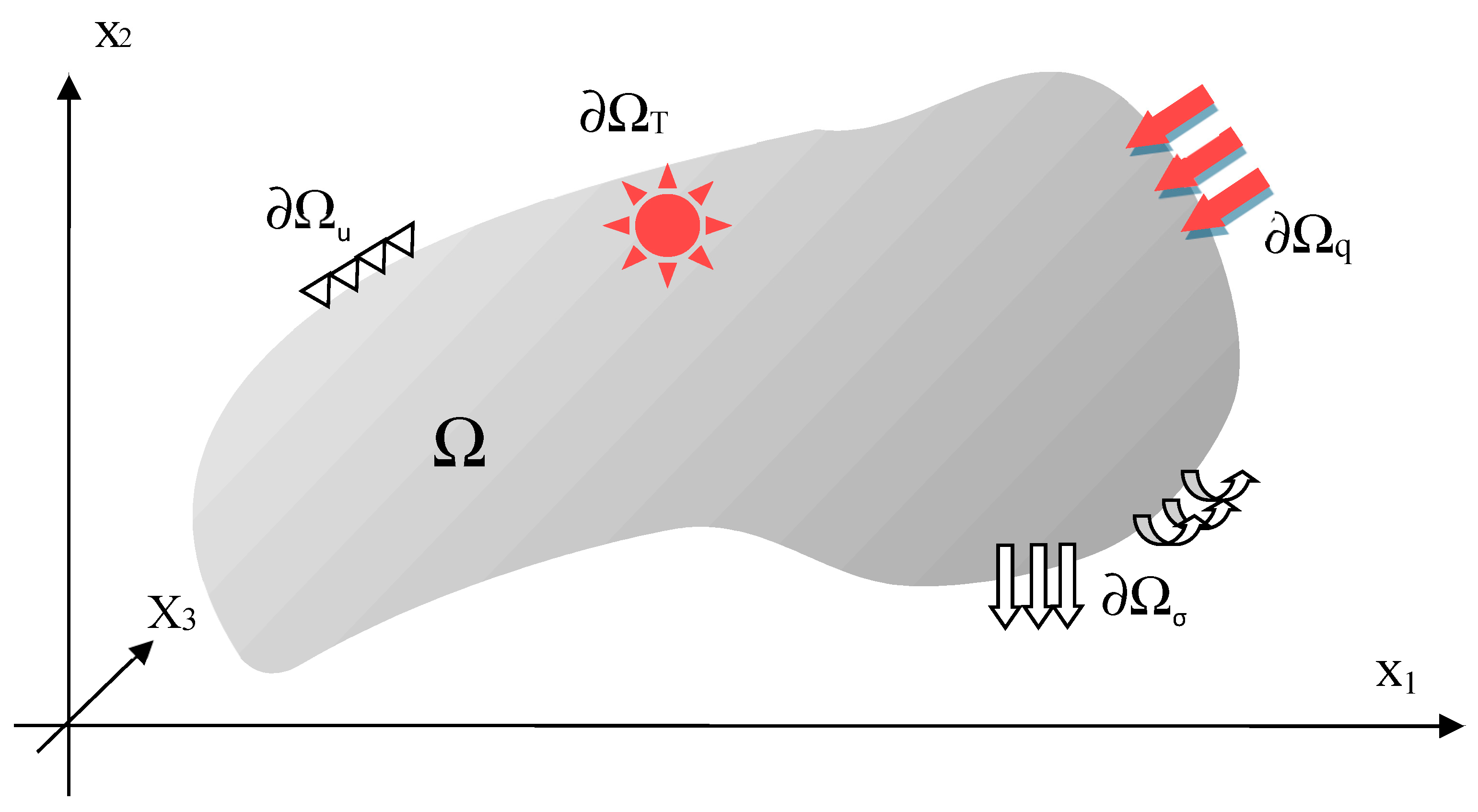
Let us consider a transient thermo-mechanical boundary initial value problem defined on isotropic and homogeneous domain Ω shown schematically below in
Figure 1.
Its mechanical part is driven by the following incremental static equilibrium equations [
52]:
with the following essential and natural boundary conditions:
This problem is solved for the displacement vector
, the strain tensor
and the stress tensor
, where the stress tensor increments
,
and denote the first and the second Piola–Kirchhoff tensors
with
All static state variables, i.e., displacements, strains and stresses are temperature-dependent, but this dependence is omitted for a brevity of presentation in all equilibrium equations. Simultaneously, a transient heat flow problem for the temperature field
T =
T(
x,τ) is solved from the following differential equation [
53]:
where
c(T) is the temperature-dependent heat capacity of the region Ω,
ρ(T) is the temperature-dependent material density of Ω,
λij(T) is temperature-dependent second-order tensor thermal conductivity, and
g is the rate of heat generated per unit volume. Traditionally,
T and
τ denote temperature field values and time, respectively.
This equation should fulfil the boundary conditions of the ∂Ω, which are given as follows:
- (1)
temperature (essential) boundary conditions
and for ∂Ω
q part of the total ∂Ω:
- (2)
heat flux (natural) boundary conditions
where
and
. The initial conditions have been introduced as
The following functional defined on
is introduced to obtain a numerical solution to the deformation problem:
whose solution is determined from the minimization of the incremental version of the potential energy stationarity principle
Analogously, one considers some continuous temperature variations
defined in the interior of the region Ω and vanishing on
. A variational formulation may be proposed here as
Let us recall the classical Finite Element Method formulation, where the displacements increments
being a continuous and differentiable function over the region Ω consisting of the geometrically continuous subsets (finite elements)
, where
e = 1,…,
E gives a complete representation of the set Ω. Let us consider the following approximation of the displacement increments [
52,
54]:
where
are the shape functions in the node
k,
represent the nodal degrees of freedom vector, while
Ne is the total number of those degrees of freedom in the considered node. Starting from the proposed approximation it is possible to express the gradients of the displacement vector as well as the strain tensor components as
and finally
The following notation has been applied in the above equations:
Now, the following elemental stiffness matrices are introduced
while the second and the third order stiffnesses are equal, respectively
Introducing
for
i = 1,2,3 into the functional
in Equation (8), applying a transformation from the local to global coordinates system, one may obtain from the stationarity condition that
Fulfilled for any configuration of the region Ω, where
,
, and
are stiffness matrix, displacement vector, and nodal loads vector, respectively. The same discretization serves for the discretization of the temperature field by the nodal temperatures vector
as [
52,
54]
The temperature gradients can be rewritten in the form
We introduce the capacity matrix
, the heat conductivity matrix
and the vector
as
and also the R.H.S. vector in the following way:
Next, let us introduce these matrixes into the variational formulation (14) to obtain the following algebraic equations system:
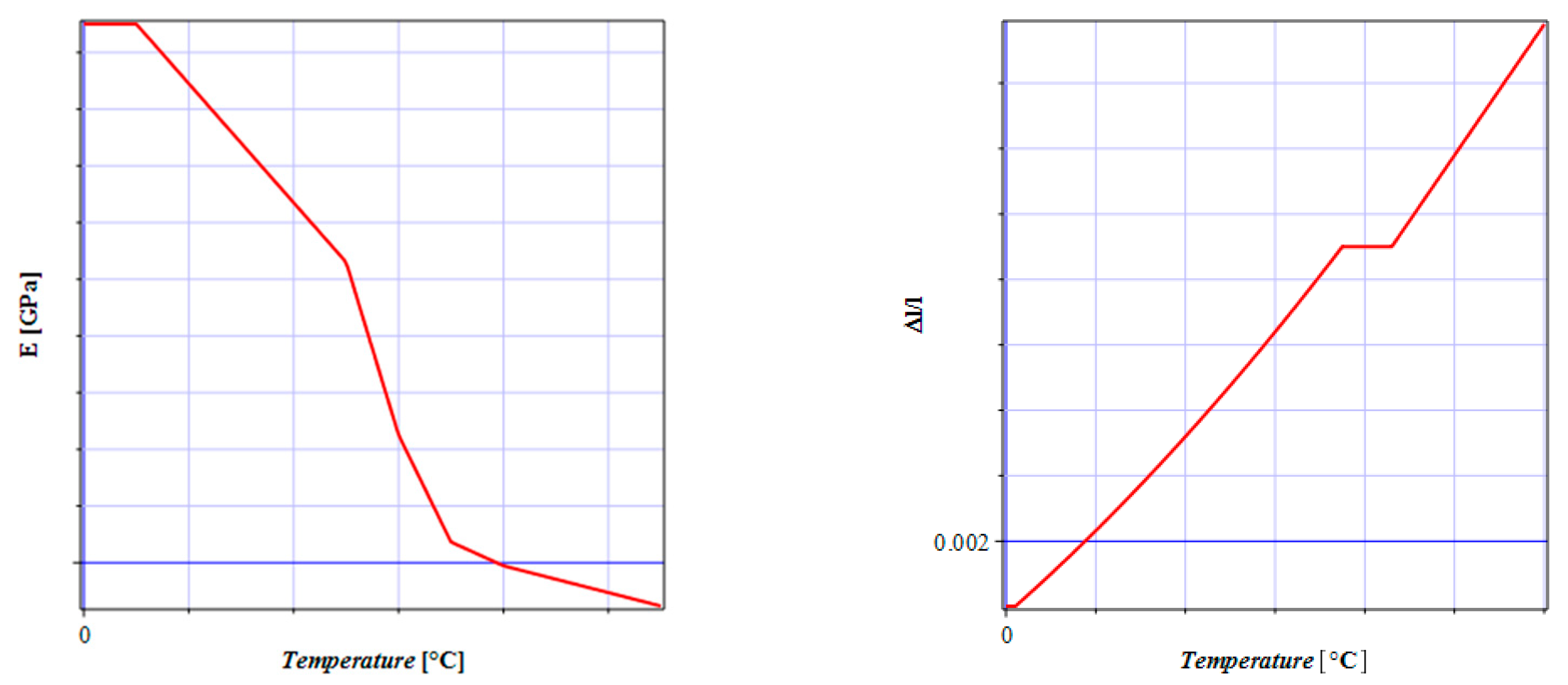
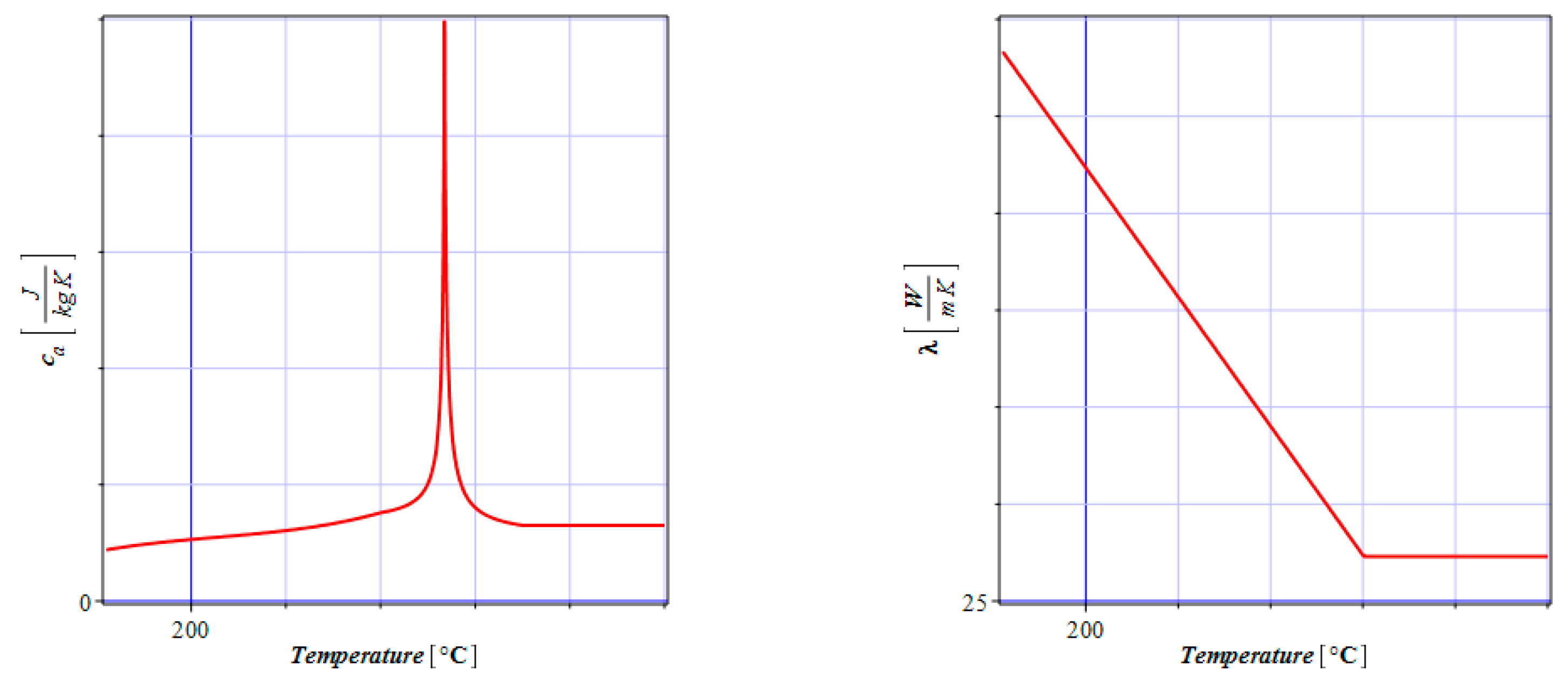
Equations (26) and (31) are finally solved simultaneously by the system ABAQUS to obtain time fluctuations of the deformations and stresses into the given boundary thermo-elasticity problem. This coupled problem is solved in a homogeneous continuous domain with no initial stresses and strains. A steel material occupying this domain shows temperature-dependent material and physical characteristics presented in
Figure 2 and
Figure 3 below. It is reported here, after experimental works included in Eurocode 3 [
2], that Young modulus as well as heat conductivity decrease while increasing temperature induced into the steel volume, quite opposite to thermal elongation, which increases. Heat capacity shows very complex behavior in this situation, especially in terms of the singularity reached close to 700 °C. This singularity results in remarkable difficulty during a solution of Equation (31), which is practically omitted by listing heat capacity at each 50 °C and numerical interpolation in-between these discrete data.
3. Probabilistic Aspects and Relative Entropy
Let us introduce the random variable
b and its probability density function as
. Then, the first two probabilistic moments of this variable are defined as [
55]
where
means the average value of
itself and
Higher probabilistic moments and related coefficients may be defined according to the classical definitions from the probability theory. The basic idea of the stochastic perturbation approach employed here is to expand all input random variables and all the resulting state functions of the given boundary initial problem via the Taylor series about their spatial expectations using the perturbation parameter
. The random function
with respect to its parameter
about its mean value is given as follows
is the first variation of a variable
about its expected value and the symbol
represents the value of a function calculated for its mean. Let us analyze further the expected values of displacement state function
defined by its expansion via the Taylor series as follows
This expansion is valid only if the state function is analytic in
and the series converges and, therefore, any criteria of convergence should include the magnitude of the perturbation parameter. A perturbation parameter here as usually in practical engineering computations is equal 1. It yields for the input random variable with symmetric probability density function in the tenth order approach
denotes the nth order central probabilistic moment of variable
b. All the terms with odd orders are equal to 0 for the symmetric random variable and the orders higher than the 10th have been simply neglected. Similar considerations lead to the expressions, such as the variance, for instance
Quite similarly, it is possible to derive higher-order central probabilistic moments from their definitions
Let us mention that it is necessary to multiply each of these equations by the relevant order probabilistic moments of the input random variable to obtain the algebraic form convenient for any symbolic computations. Based on the classical definition of the variance we can calculate the coefficient of variation, skewness, and kurtosis as follows
It should be mentioned that at this stage the proposed procedure is still independent of a choice of the initial probability distribution function, however, a satisfactory probabilistic convergence of the final results may demand various lengths of the expansions for random variables with different distributions. A common implementation of the Monte-Carlo simulation, semi-analytical approach, as well as higher order stochastic perturbation technique in the system MAPLE was possible thanks to the Least Squares Method polynomial recovery of the structural displacements with respect to the input uncertain parameter b.
Finally, the reliability index is to be determined to measure the structural safety of the given case study of the beam under fire conditions. The engineering codes (such as Eurocode 0) advise applying the FORM theory, where one calculates
E[R] denotes here the maximum acceptable displacement of a beam according to Eurocode 3, and E[E] is the expected value of extreme displacement calculated based upon the iterative generalized stochastic perturbation technique. It is well known that the FORM approach has some limitations, so that higher order theories have been developed such as the Second and even Third Order Reliability Methods (SORM and TORM), especially because of the linear character of the limit function in the FORM technique. This seems to be unjustified in many practical applications and undoubtedly fire simulation is one of them. Further, the main mathematical methodological difficulty is that both distributions, of R and of E, are assumed as Gaussian here, which may be far from the experimental evidence and even misleading in the view of many theoretical studies and computer simulations.
This was a reason to seek for another concept to assess structural reliability in the presence of fire and to define the reliability index using probabilistic distance in-between two distributions of structural resistance and of structural extreme effort. One of the available mathematical models is the Bhattacharyya theory [
40], which proposes for two different PDFs, namely
pR(
x) and
pE(
x), the following probabilistic distance measure:
where associated with structural resistance and probability function related to structural effort, respectively. Such formula enables the application of two different probability distributions of practically any nature and the given set of their parameters; further application of the analytical integration using some computer algebra system may lead to the desired numerical value. However, this formula can be simplified in the case of two Gaussian distributions with the given expectations and standard deviations (
μ(R),
μ(E), and also
σ(R),
σ(E), correspondingly). There holds
Another problem is the upscaling of the variability interval of reliability indices obtained as the result of Equation (41) (or (42)) to contrast them with the values resulting from the FORM approach. The main idea would be to apply this mathematical apparatus with its theoretical importance, but to retain the existing engineering codes recommended minimum values of the reliability indices. Without such an upscaling direct determination of the reliability index, it would never show any extremes separating safe and unsafe design and/or exploitation of the given structure. Some preliminary computational experiments enable to propose the following rescaling of such a reliability index to numerical values comparable with the existing codes:
Both square root function as well as the multiplier preceding this function has been taken to make the first component, free from logarithmic function as close as possible to Equation (40); further numerical analysis would check an efficiency of such a modified reliability index. Computational implementation of the aforementioned approach has hybrid character and uses both the FEM system ABAQUS Standard, and also computer algebra package MAPLE. ABAQUS Standard fully coupled thermoelastic analysis is run multiple times to have the series of temperatures, stresses, and displacements obtained for the few different input fire temperatures. Then, these discrete results are in vector formats transferred to the MAPLE system, where the Least Squares Method procedures enable to recover polynomial approximations of these state functions with respect to fire temperature. Finally, this fire temperature is randomized according to the Gaussian distribution with the given mean value and given variability interval of the coefficient of variation. Polynomial approximations of temperatures, stresses, and displacements together with a triple implementation of probabilistic analysis return the basis probabilistic characteristics (i.e., expectations and standard deviations) of the state functions. Finally, two different reliability indices presented in Equations (40) and (43) are determined as the functions of fire exposure time.
4. Computational Illustration
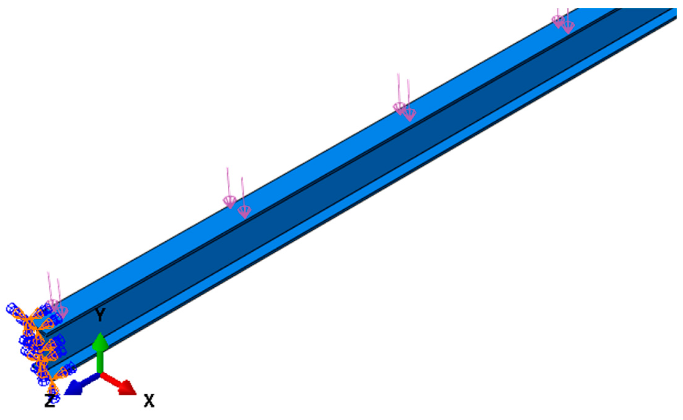
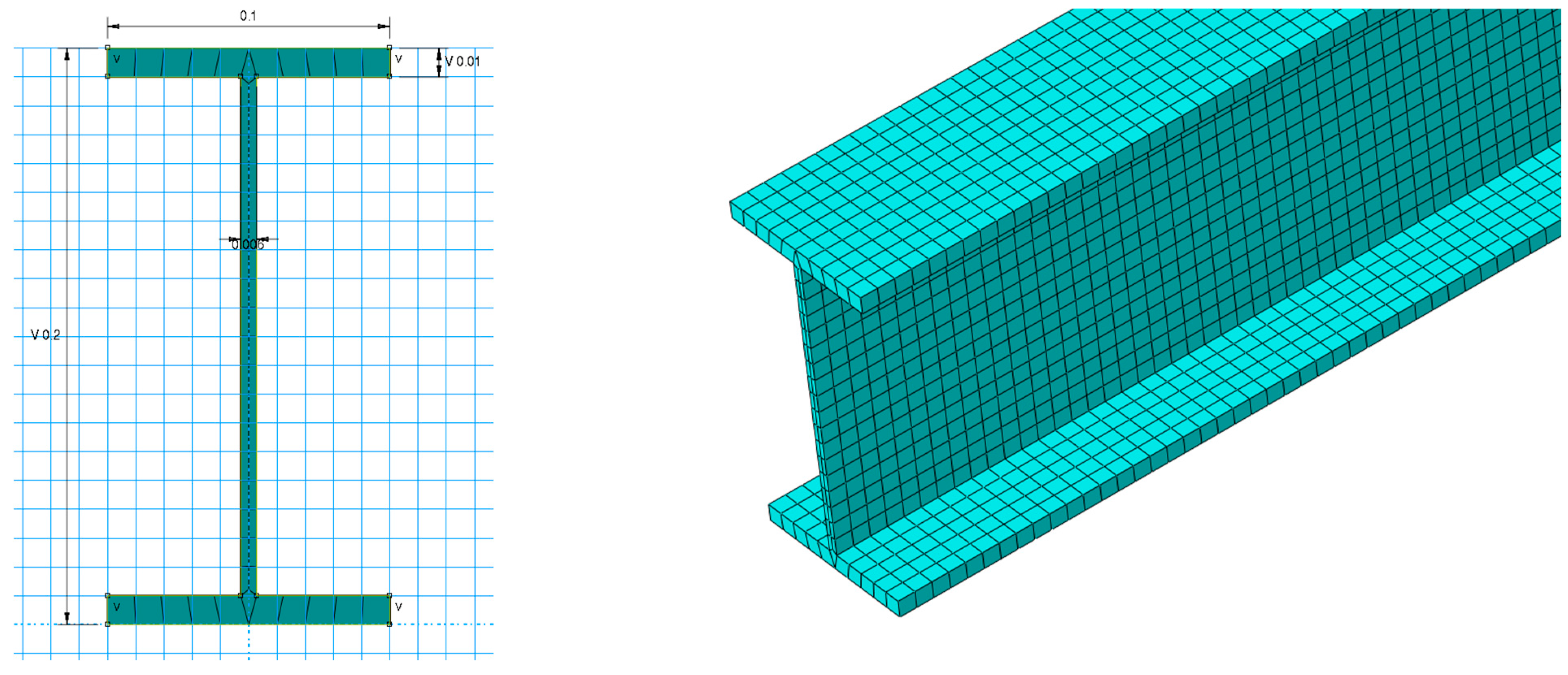
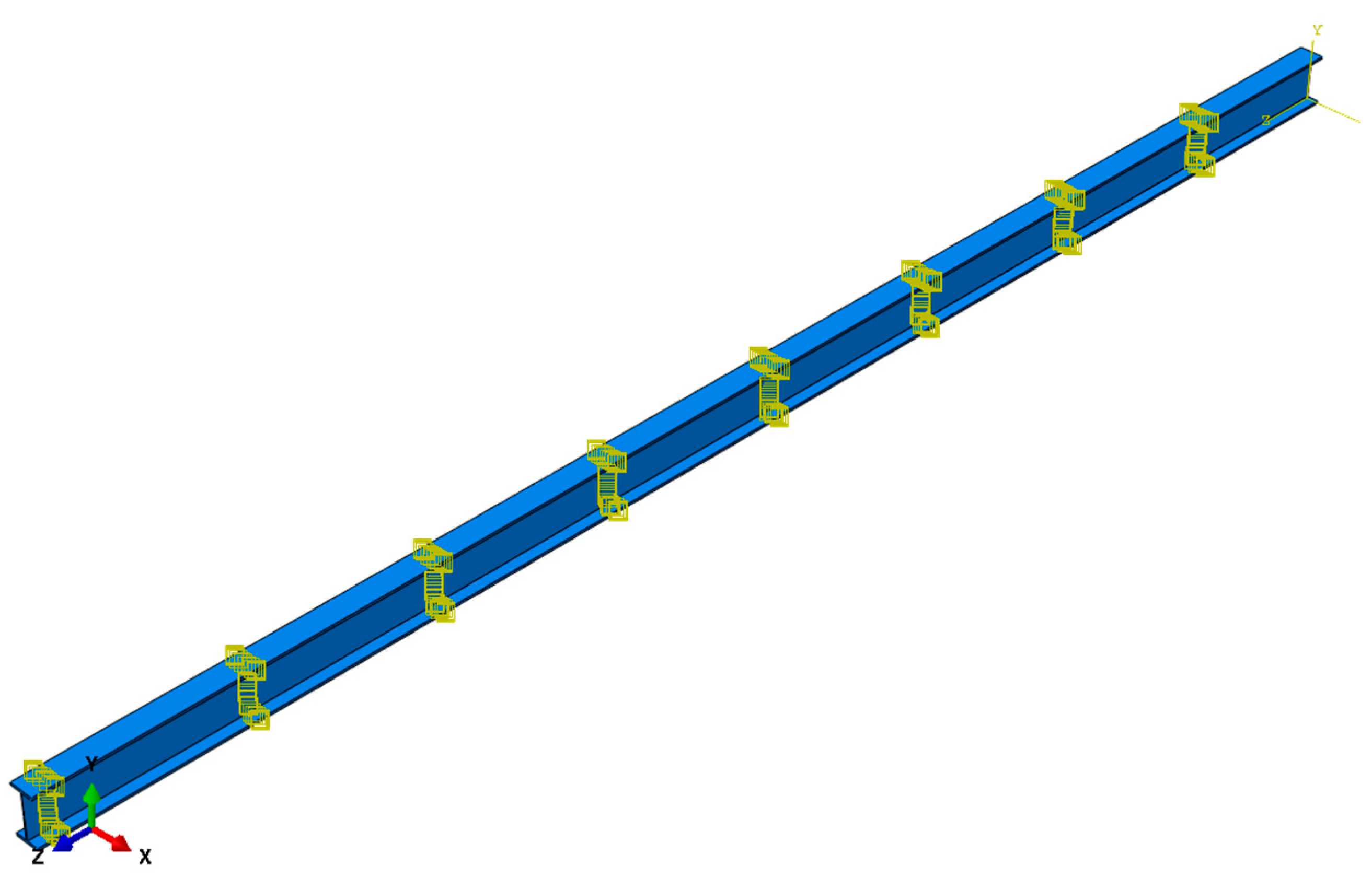
The numerical example consists of the 6m both ends fixed steel I-profile beam with linear load applied to top flange equal 2.0 kN/m (
Figure 4), whereas its cross section and the FEM discretization have been shown in
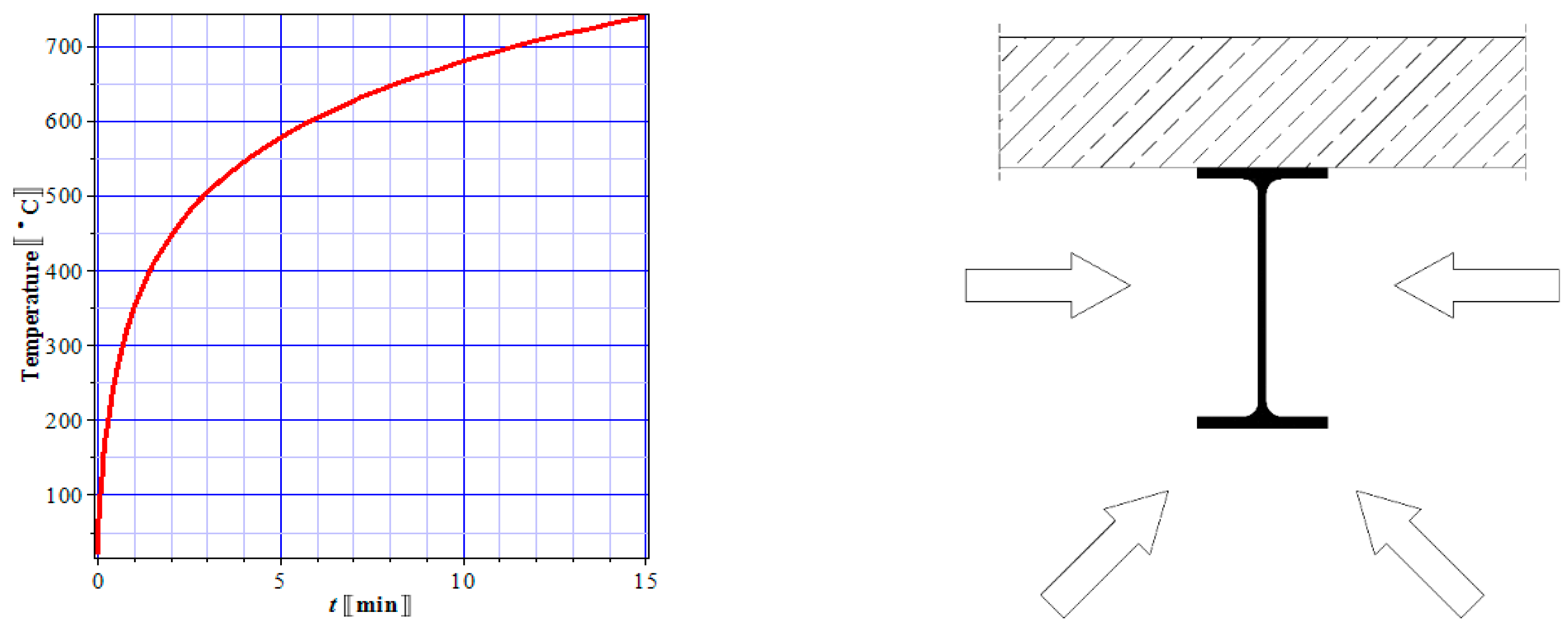
Figure 5. The mesh consisting of 34,800 brick finite elements has been used; they are denoted in the system ABAQUS as C3D8T: the 8-node thermally coupled brick, tri-linear displacement, and temperature. The edge length of each brick element is less than 10 mm and it guarantees quite smooth approximation of stress distribution throughout the web. The thermal load has been adopted from the Standard ISO fire curve (
Figure 6). According to Eurocode fire fumes after time t
f = 15 min are about 740 ºC. This thermal load has been applied to each side of the cross-section except the top flange where the concrete slab lays according to the given fire scenario (
Figure 6). Surface radiation and surface film conditions as thermal loads have been applied in this model (
Figure 7). All material parameters are fully temperature-dependent and the fully coupled transient temperature-displacement incremental analysis has been used with the full Newton solution technique. The total time period of numerical simulation has been set as 900 s. The initial increment size is 0.01 step time, in this case, the minimum increment size is 0.0001 of the step time, and the maximum increment has been fixed as a single second.
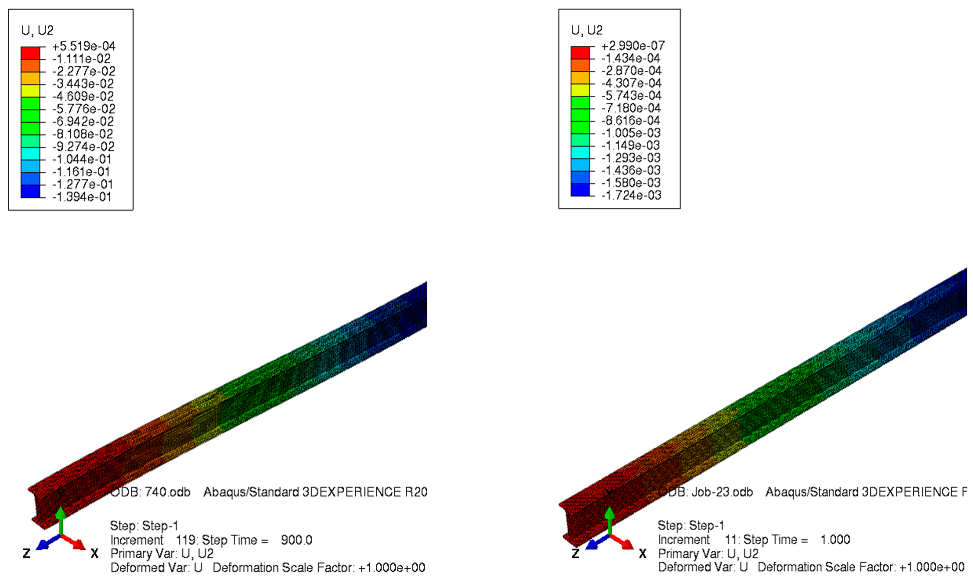
Figure 8 shows a comparison of this beam deflection under the given fire conditions (left diagram) and without a fire (right diagram). It is noticeable that fire heating increases the extreme deflection at half of the beam span more than four times (13.0 cm) than its admissible value (3.0 cm); maximum deflection in this case of no fire is less than 2.0 mm. One concludes that extreme deformation in the beam under fire is two orders larger than for the beam with no temperature attached (analytical approximation following basic equations of strength of materials appears to be quite efficient). The second major difference in-between these two models is that a beam subjected to fire shows remarkable deformations close to the supported area, whereas the beam without fire loadings has these deformations negligibly small. Next,
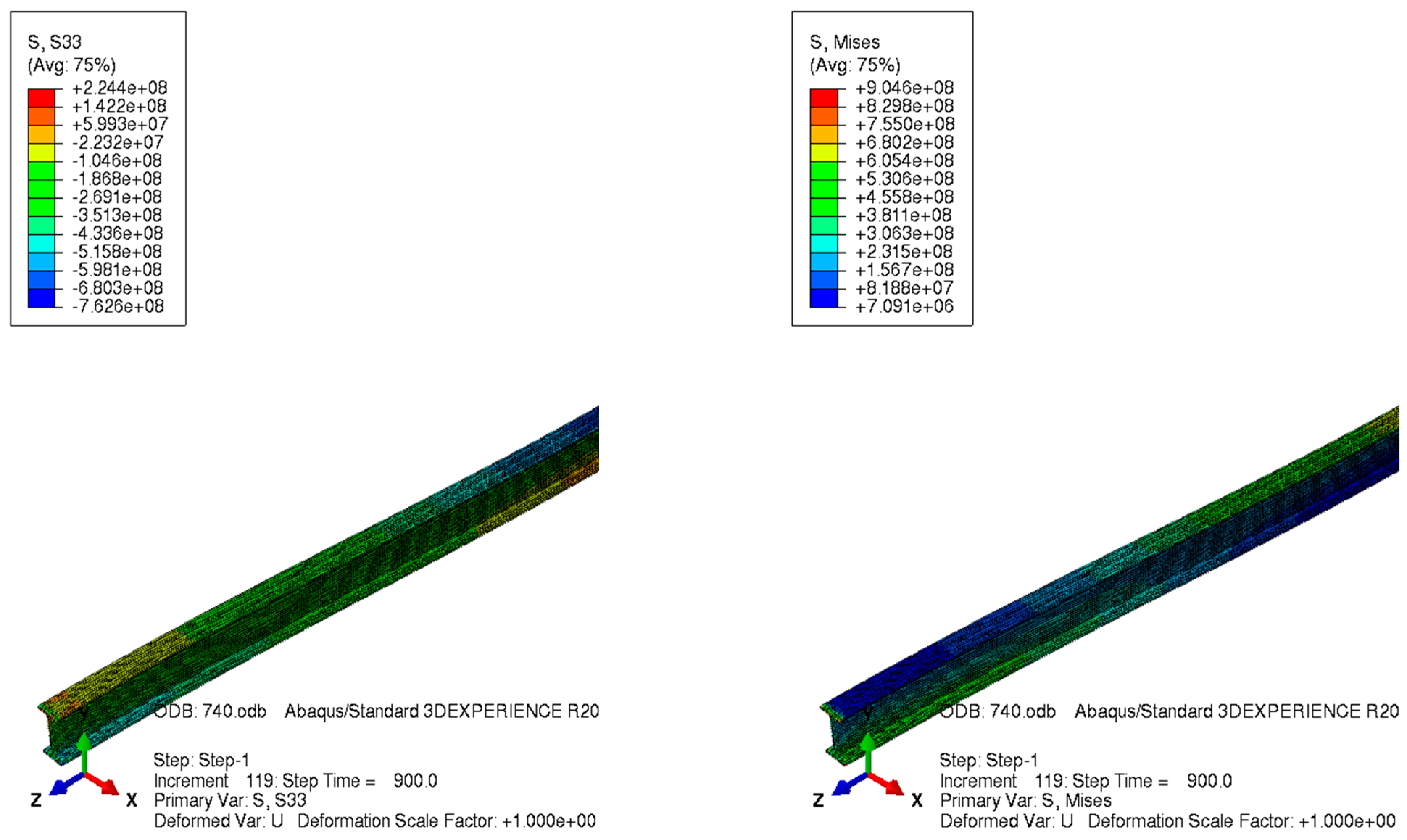
Figure 9 reports normal stress marked as S33 (left diagram) and the reduced von Mises stress (right diagram). Von Mises stresses are almost 4 times larger than the longitudinal stresses in this specific case and both stress fields exhibit quite different distributions along the beam and throughout its cross-section.
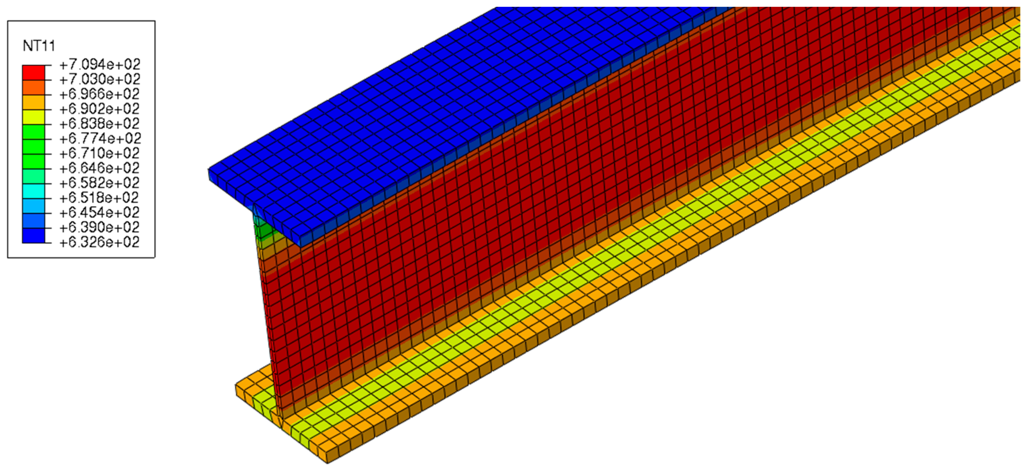
Figure 10 shows for a completeness temperature distribution at the steady-state (at the end of the beam heating by a fire) and one compares with an engineering intuition that the thinner web accumulates definitely more heat than the relatively thicker rest of the beam.
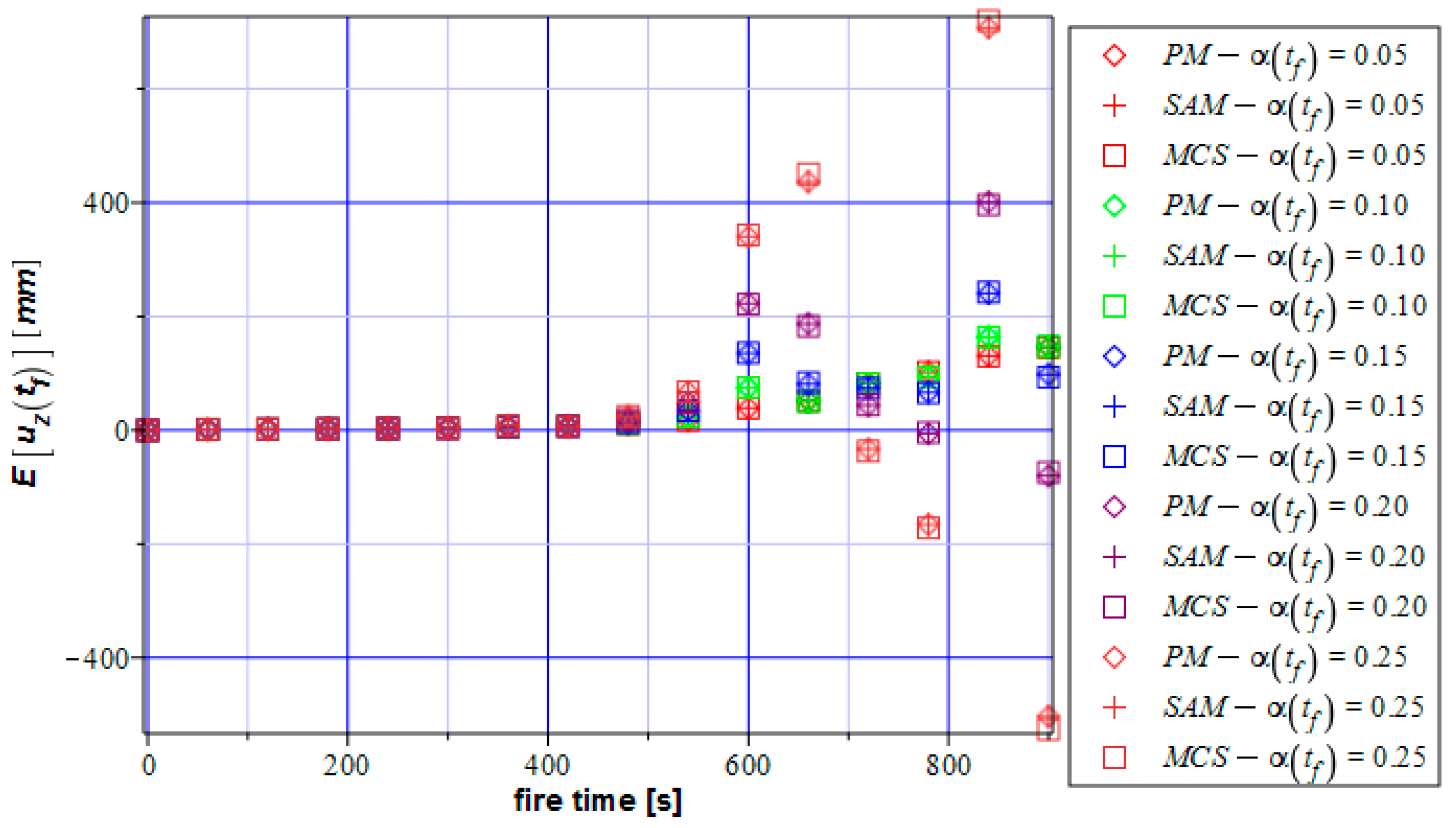
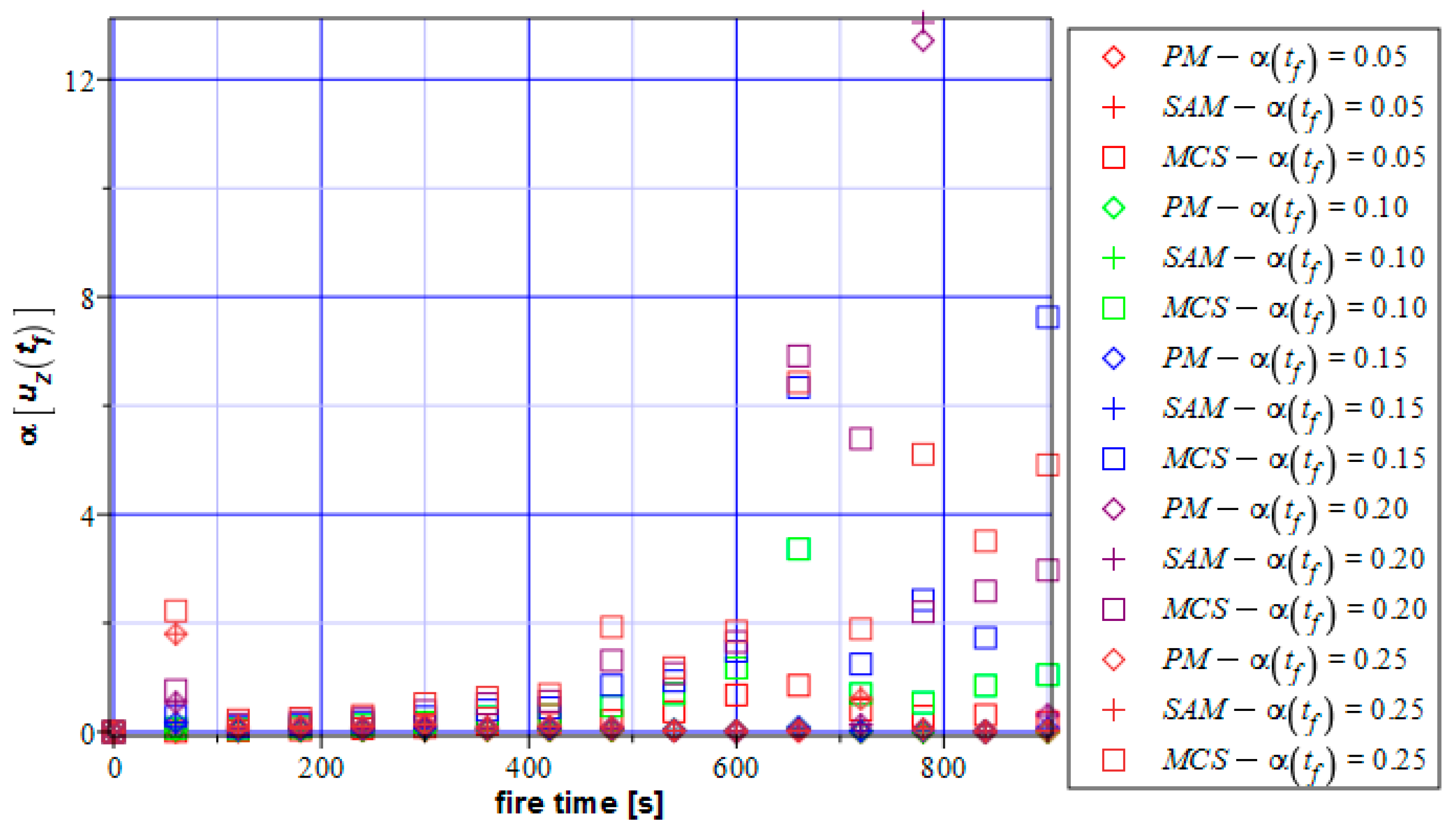
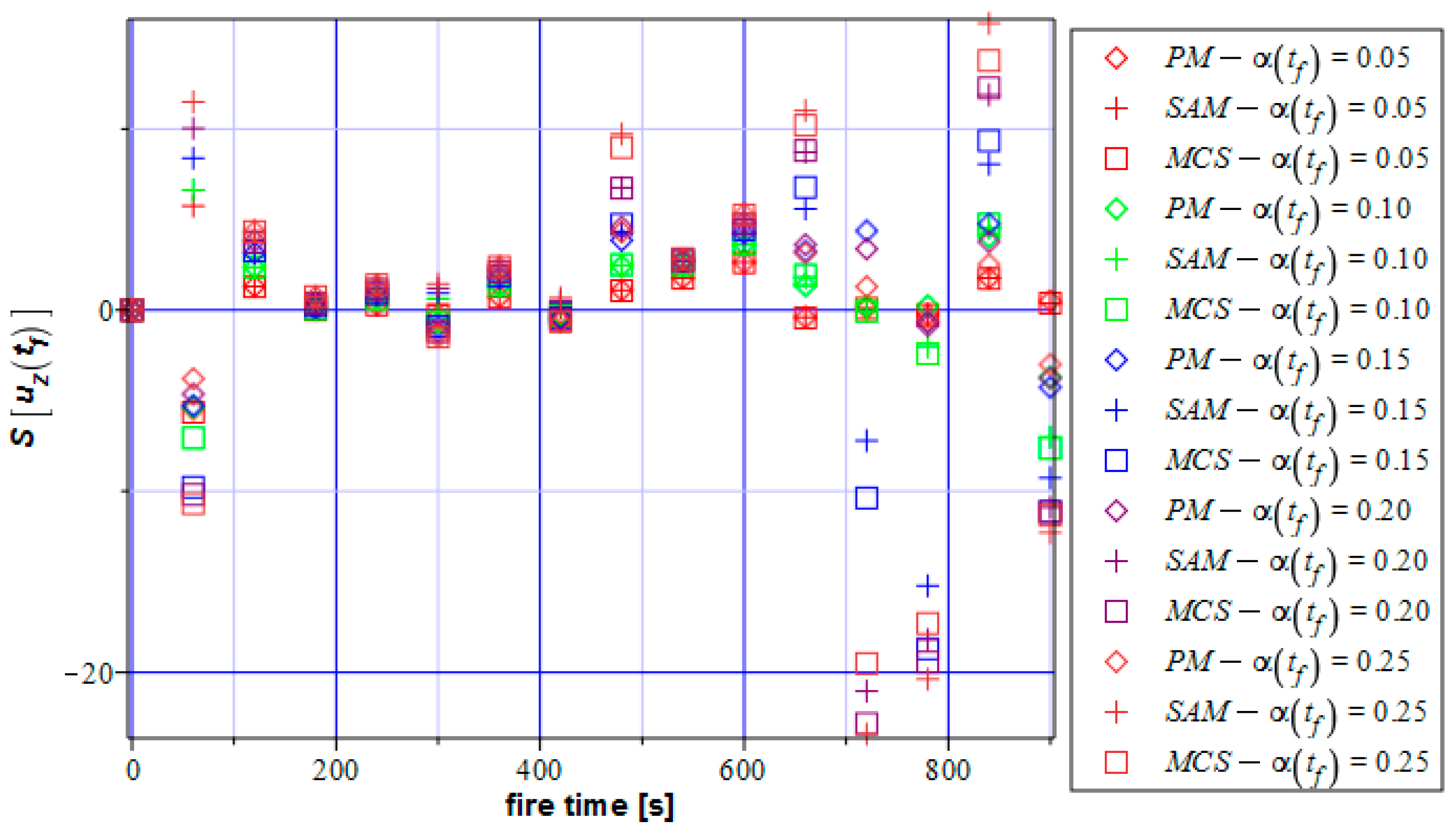
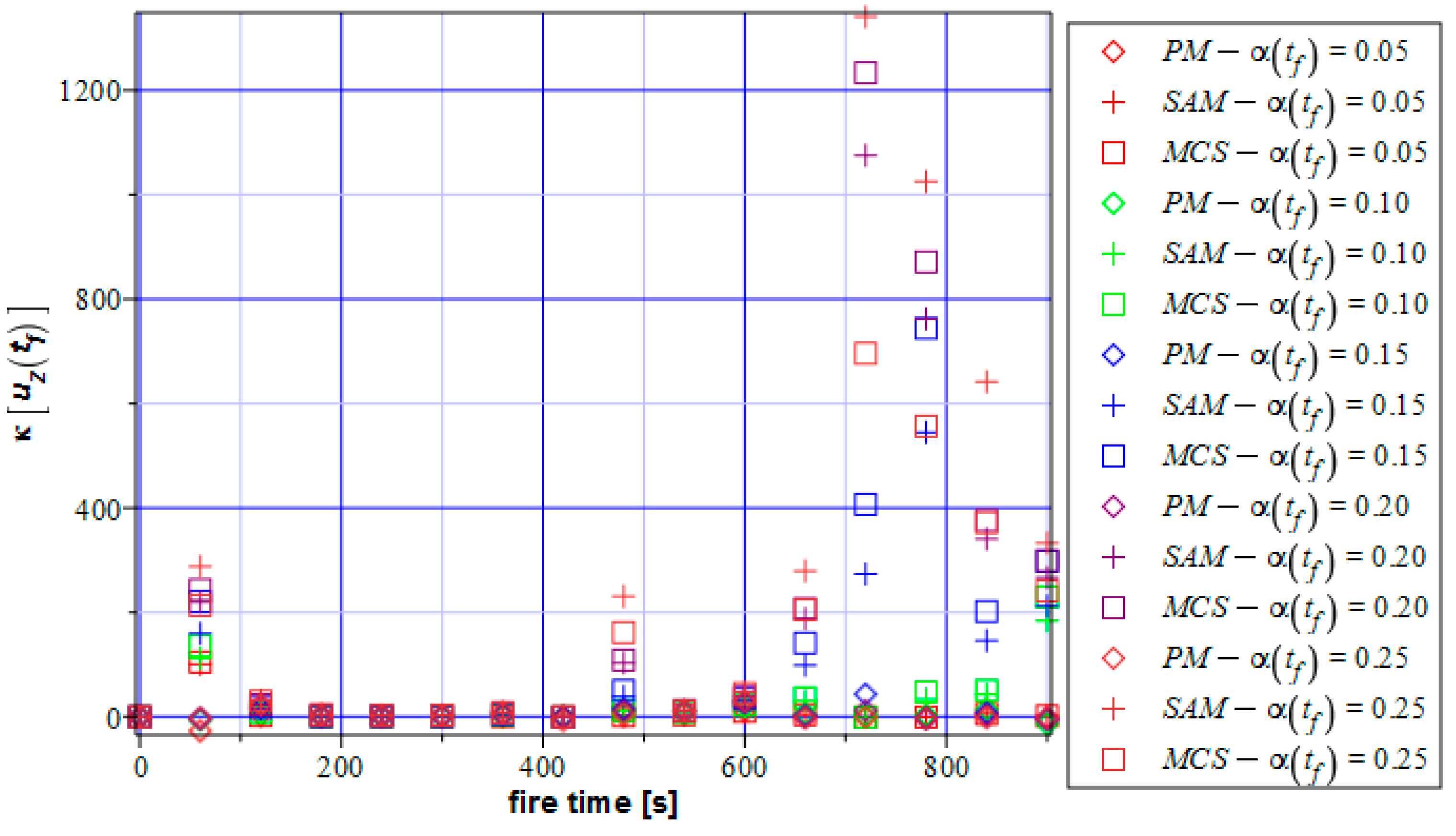
Further results concern probabilistic characteristics of the structural response, which include expectations, coefficients of variation, skewness, and kurtosis of displacements shown in
Figure 11,
Figure 12,
Figure 13 and
Figure 14, correspondingly. They have been computed using three different probabilistic methods, namely the perturbation method (abbreviated as a PM here), the semi-analytical method (SAM), and also using the Monte-Carlo simulation (MCS); they have been shown all as the functions of the input coefficient of variation ranging from 0.0 until 0.25. They concern extreme vertical displacements obtained at the half of the beam structure for the needs of further reliability assessment according to the Serviceability Limit State (SLS). First of all, it is seen that the first two moments are stable until t = 500 s, and then they start to diverge; initially, both moments equal almost 0. Generally, three different probabilistic numerical methods coincide in the case of the first two probabilistic characteristics with each other until α = 0.20. Higher order statistical characteristics are more dispersed—they exhibit both numerical values very close to 0, which start to diverge at about t = 500 s. This can be interpreted that until this time moment of the fire exposure, the resulting displacements can be approximated as Gaussian, which means that both the FORM expression for the reliability index as well as its relative entropy counterpart proposed by Equation (43) are justified very well. Finally, one can notice that all three probabilistic methods coincide very well until
α(
tf) = 0.10.
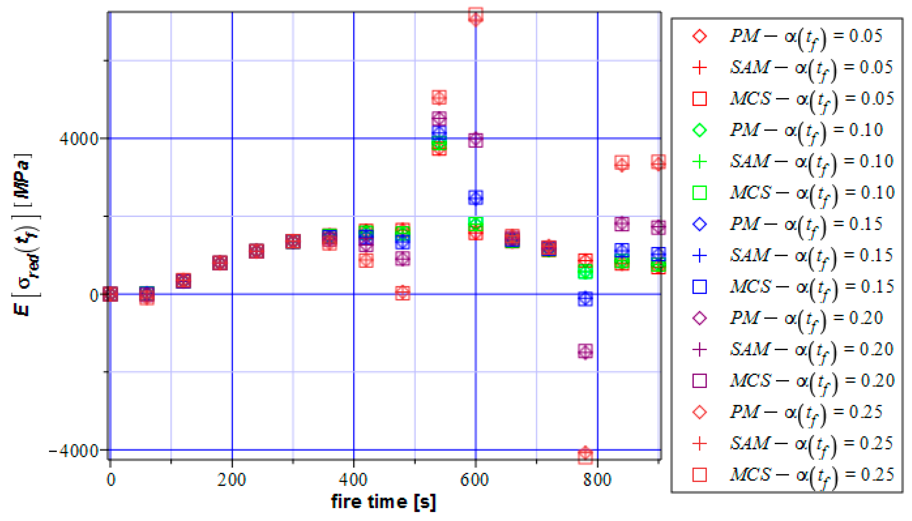
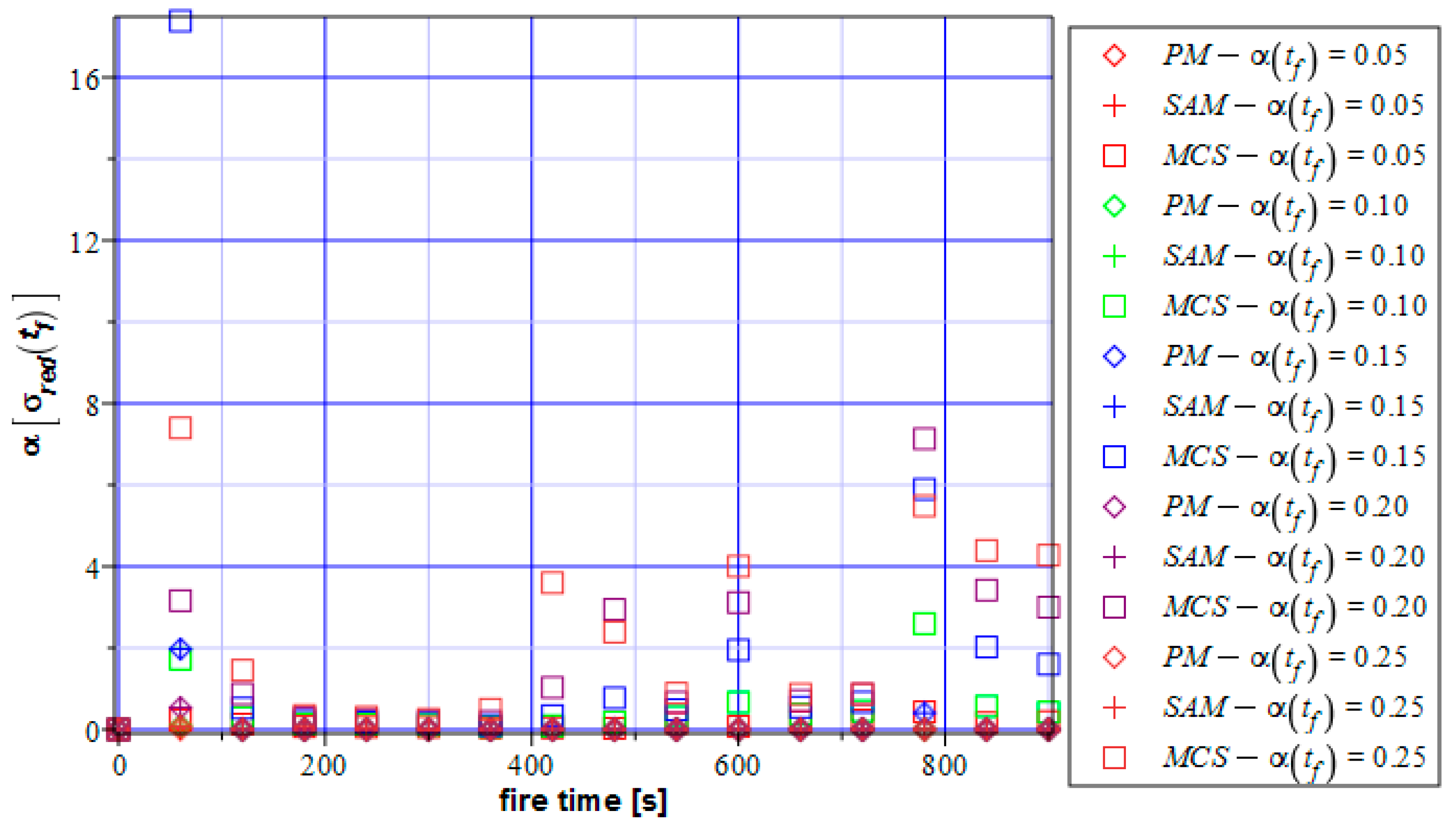
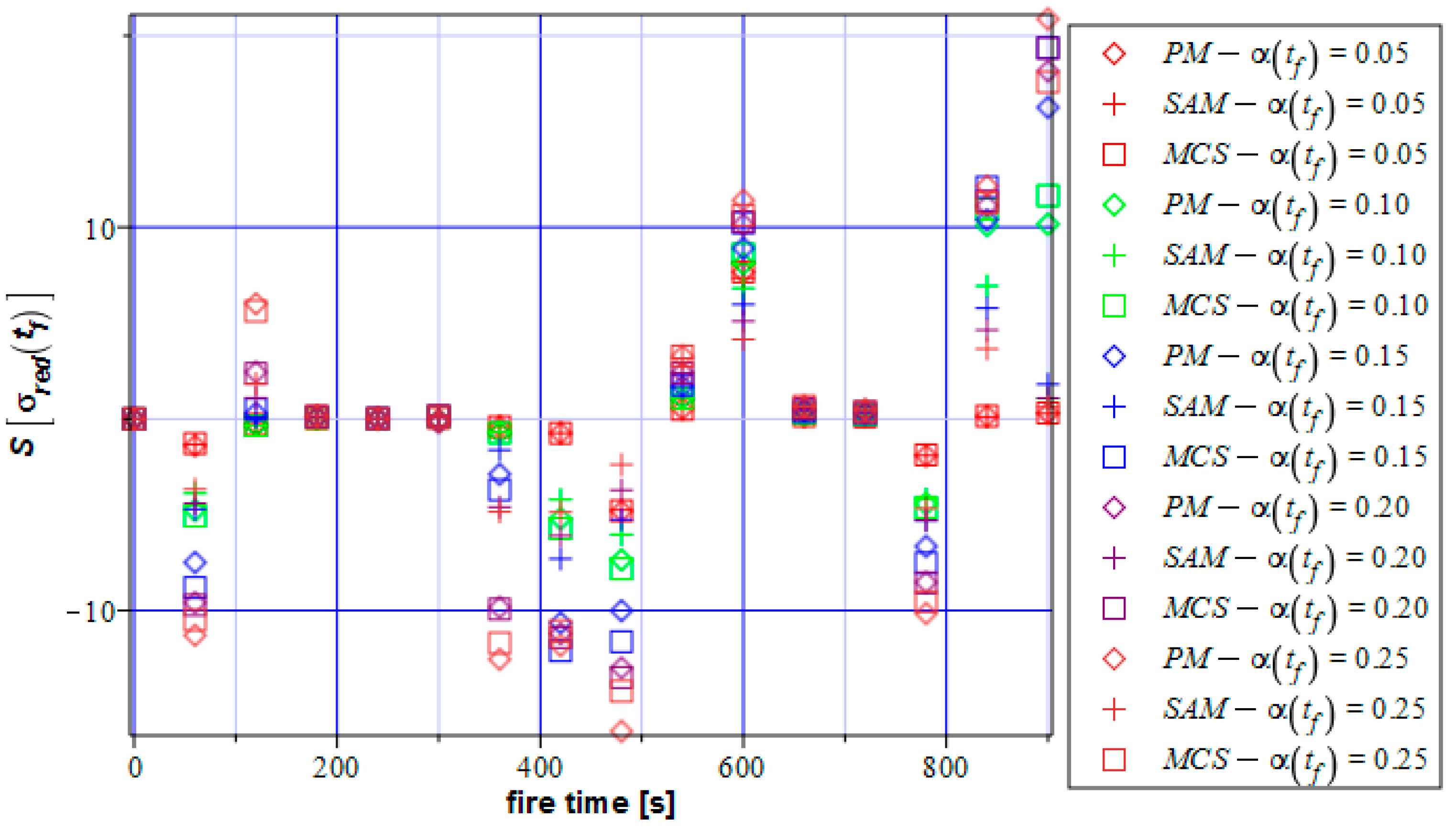
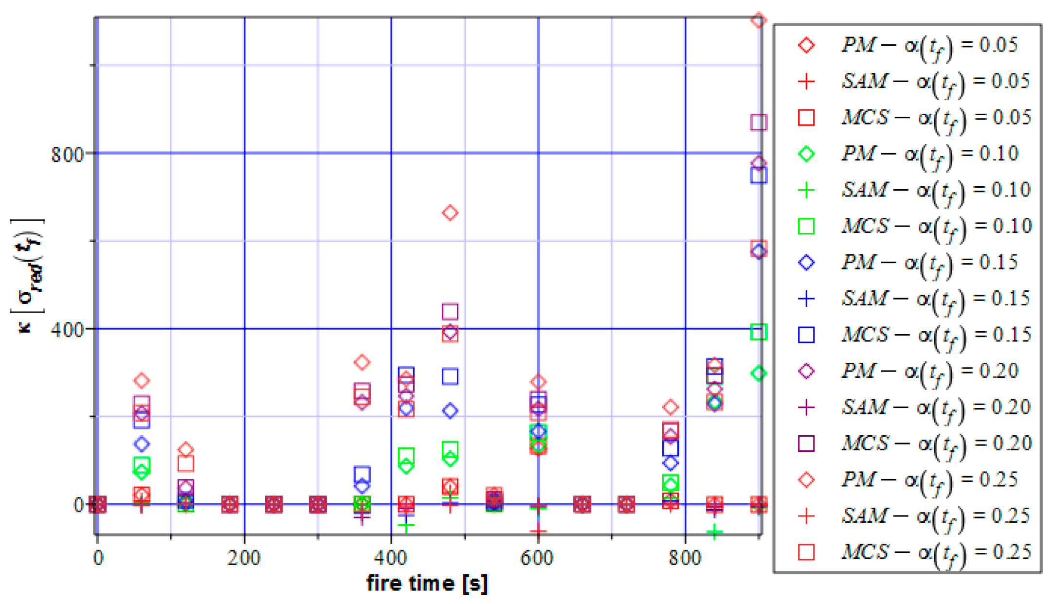
The next set of probabilistic characteristics computed for the reduced von Mises stresses is given similarly in
Figure 15,
Figure 16,
Figure 17 and
Figure 18. They have been collected here as decisive in the calculation of the reliability index in the Ultimate Limit State (ULS). The expected values increase monotonously from 0 until the same moment t = 500 s; then, they exhibit large fluctuations, although all three probabilistic methods return the same numerical values. The reduced von Mises stresses start to highly depend upon the input coefficient of variation for the fire exposure time t > 500 s, which is an observation quite unusual for elastic problems with any uncertainty. A little bit different conclusions can be drawn from the results contained in
Figure 16—the output CoVs keeps very close to 0 during the entire fire heating process showing some numerical discrepancies almost at the beginning of this process (t = 50 s) as well as its end (t = 800 s). Higher order statistics are rather distant from 0 (see
Figure 17 and
Figure 18), so they cannot be efficiently modeled as Gaussian and need larger numerical effort. A coincidence of Monte-Carlo simulation, the semi-analytical method as well as the stochastic perturbation technique is worse and can be assumed
α(
tf) = 0.05. This is a quite expected result because probabilistic characteristics of the stresses are calculated based on probabilistic moments of displacements (since displacement-version of the FEM is used) and of probabilistic characteristics of the constitutive tensor (additionally depending on the nodal temperatures).
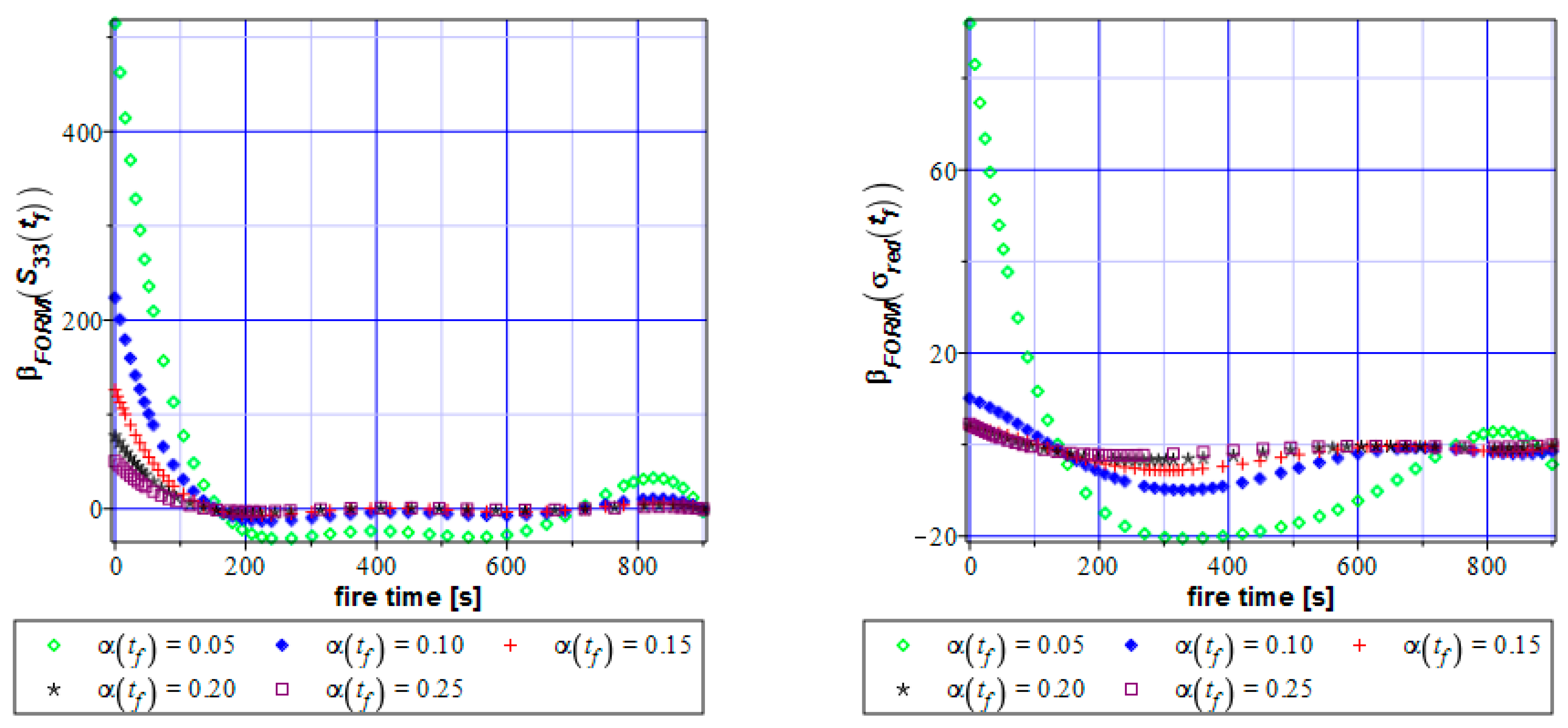
Higher order statistics of the reduced stresses are definitely distant from 0 during fire exposure time, so that these stresses cannot be approximated with the Gaussian distribution. Therefore, the FORM index given in Equation (40) includes a remarkable modelling error, whereas relative entropy should be calculated here using the general analytical formula (42). Further numerical results concern reliability analysis of the given structure, so that
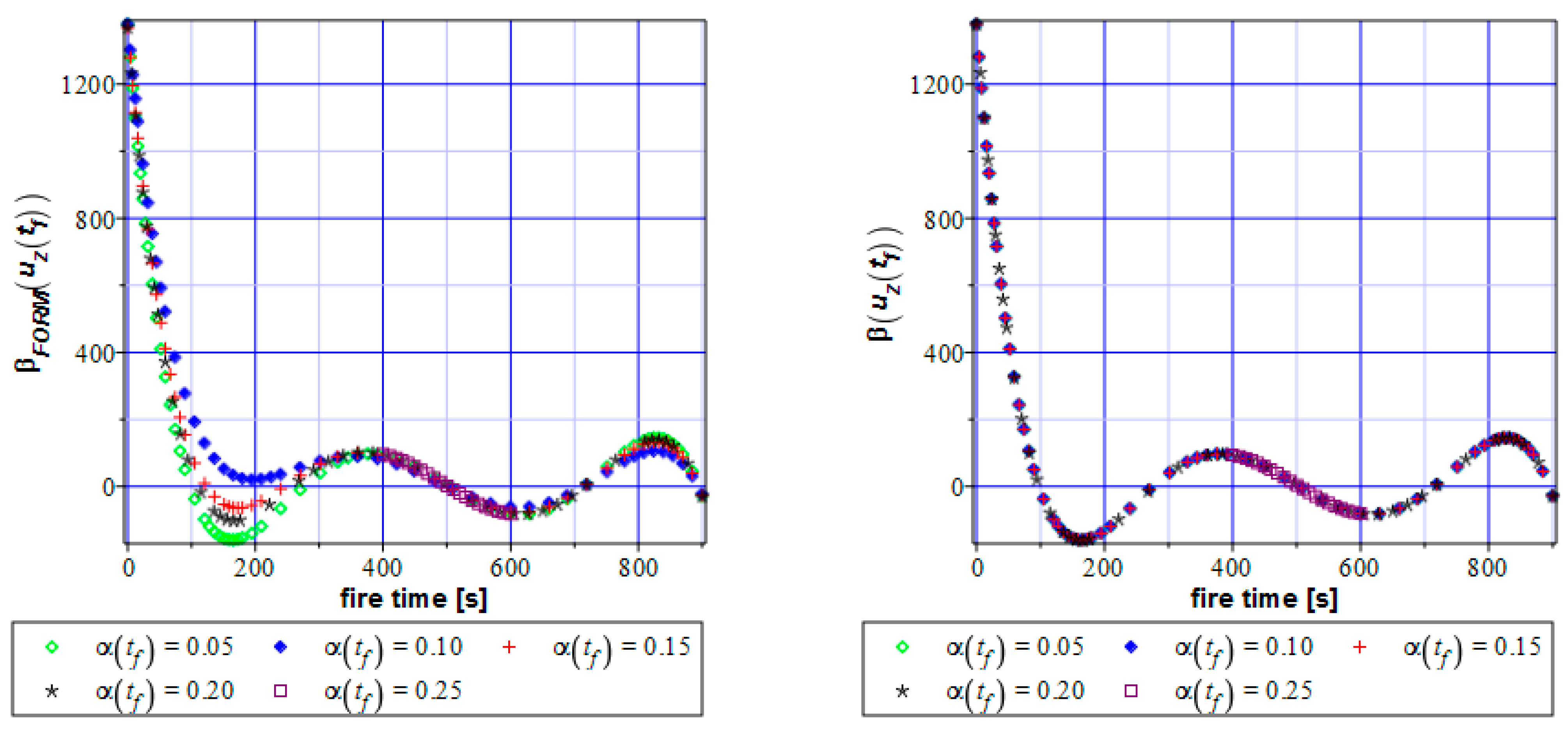
Figure 19 contains the key results in this study and presents a comparison of the reliability indices determined using the FORM approach (left graph) with these calculated thanks to the Bhattacharyya relative entropy. They are both plotted as the functions of the fire exposure time and are related to the Serviceability Limit State. This is because previous results document well approximation of the distribution of the displacement by the Gaussian PDF; this is not the case with the reduced stresses, so their reliability has been discussed in
Figure 20 using the FORM index only. As one could expect, these time fluctuations of reliability indices have typical exponential decay in the first stage of fire heating, but then, after reaching critical and 0 values, exhibit further oscillatory character. This part is interesting from the numerical point of view and has no practical importance and the structure lost its reliability. Such a wavy character is totally absent for civil engineering structures subjected to, i.e., static loads and some stochastic ageing process, when reliability decreases monotonously.
The very important conclusion following the comparison of the two graphs in
Figure 19 is that the FORM index and relative entropy variations show the same character and extreme values location. The most important conclusion is that they cross the admissible value at almost the same time as a fire accident, which means that structural safety analysis results in both cases in the same evacuation time. Further, it is seen that the FORM analysis results in a few times higher reliability index at the very beginning of the fire accident. This can be meant as some overestimation of the realistic reliability, but this difference is meaningless for structural design. A very interesting result is that the FORM index is more sensitive to the input uncertainty level, whereas the relative entropy shows almost no such sensitivity.
The reliability index in the ULS analysis shows less waviness above the reliability limit. It does not affect the conclusion and structural safety—it concerns computational aspects rather. A contrast of
Figure 19 and
Figure 20 results in a conclusion that the ULS is decisive for the overall safety of this element—it seems that the given beam faster falls into the plastic regime than approaches the admissible deformations at half of its span. This conclusion is a little bit out of the probabilistic analysis, nevertheless, the stochastic reliability study confirms an engineering observation. This notice is supported mainly by the reduced von Mises stress time fluctuations. Evaluation of the beam safety from the normal longitudinal stresses may lead to an improper conclusion that the ULS and the SLS exhibit almost the same failure time.
A more detailed comparison of the classical FORM approach with the proposed new one based upon the relative entropy has been provided in
Table 1 below (β
FORM(u
z(t
f))) and relative entropy approach (β(u
z(t
f))). Both reliability indices have been compared with each other throughout the entire fire accident simulation time for the few different values of input coefficient of variation. There is no doubt that both methods return almost the same values (positive and negative also) for any input statistical scattering. Furthermore, a failure time defined as the moment of fire duration when the reliability index falls down below the admissible values suggested in the designing codes (t = 80 s) in both methods is also almost the same. It seems that the rescaled relative entropy calculated from Equation (43) enables to predict fire safety with the use of the existing engineering codes.
The data presented in both
Table 1, and also in
Figure 19 and
Figure 20 demonstrate that steel beams without any fire protection are extremely sensitive to fire temperatures. A sensitivity of its deformation is of course a few times higher than of the ULS limit function, which is confirmed by the negative reliability indices detected in case of the SLS. It is important that both reliability approaches return the same qualitative results.
Finally, it should be noticed that quite a satisfactory accuracy of both probabilistic simulations and reliability analysis shows that the methodology presented could be applied to other types of steel structures and further applications towards aluminum alloys may be taken into account. Undoubtedly, this approach would be closer to industrial applications when the phase change (from solid to liquid) could be accounted for; this needs brand new implementations in the system ABAQUS. It should be mentioned that the civil engineering designing codes still do not include any statements enabling efficient engineering reliability concerning fire safety (neither for steel nor for concrete or traditional structures). On the other hand, closer interoperability of the FEM system ABAQUS, with the computer algebra packages such as MAPLE should be also achieved.


