A Novel Generic Diagnosis Algorithm in the Time Domain Representation

Abstract

The health monitoring of a system remains a major issue for its lifetime preservation. In this paper, a novel fault diagnosis algorithm is proposed. The proposed diagnosis approach is based on a unique variable measurement in the time domain and manages to extract the system behavior evolution. The developed tool aims to be generic to several physical systems with low or high dynamic behavior. The algorithm is depicted in the present paper and two different applications are considered. The performance of the novel proposed approach is experimentally evaluated on a fan considering two different faulty conditions and on a proton exchange membrane fuel cell. The experimental results demonstrated the high efficiency of the proposed diagnosis tool. Indeed, the algorithm can discriminate the two faulty operation modes of the fan from a normal condition and also manages to identify the current system state of health. Regarding the fuel cell state of health, only two conditions are tested and the algorithm is able to detect the fault occurrence from a normal operating mode. Moreover, the very low computational cost of the proposed diagnosis tool makes it especially suitable to be implemented on a microcontroller.

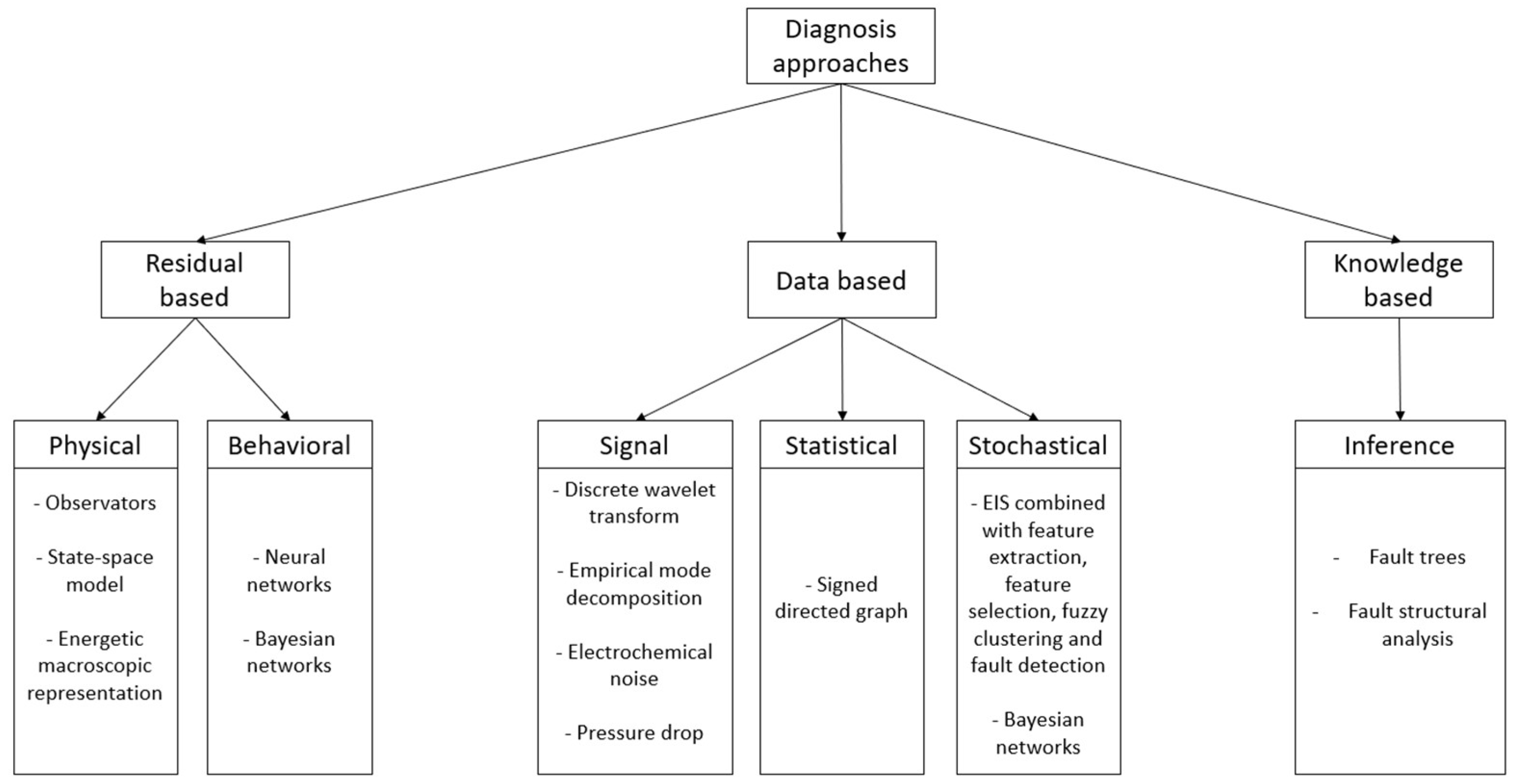
1. Introduction

The issue of a diagnosis process lies in its ability to detect and isolate a fault as early as possible. It must also be able to be integrated into a fault tolerant control (FTC) strategy to manage the system’s state of health (SOH) even under faulty conditions. As more the diagnosis result is accurate, as more the SOH can be maintained.

A previous literature review, depicted in [1], summarize all possible approaches for fault diagnosis. This paper underlined the importance of developing diagnosis tools regarding their ability to degrade a system. Several levels of degradation can be considered. First, transient performance degradations due to a fault occurrence are the major issue for real-time characterization before any irreversible loss of performance. Then, irreversible degradations that can occur under faulty operations and cannot be recovered have to be diagnosed to reduce the degradation process and to find a better operating point. For this purpose, residual-based, data-based, or knowledge-based approaches are the three main methodologies for the implementation of a diagnosis tool. The authors present this diagnosis method distribution through a graph which is shown in Figure 1:

Regarding the residual-based methods, two ways are available for diagnosis development: physical or behavioral methods. Both approaches concern the set-up of a model which reproduces the behavior of the real system. A deviation of the physical system from the model is then interpreted as a fault occurrence. For instance, in [2], the authors proceed to a residual-based diagnosis to detect and identify a faulty condition for a three-level converter. Their approach consists to compare the voltage difference between measured values and values obtained through differential equations. The authors conclude their study by stating that their diagnosis method manages to not only detect and identify a fault occurrence but also to compute the fault level (also called fault magnitude in this paper). However, the drawback of this kind of method concerns the lack of consideration of the system aging in the physical equation. Therefore, even if the method remains robust and relevant for youthful systems, these model-based approaches need an identification process that is not easy to perform.

The limitation due to the aging phenomena could also be taken into consideration for the knowledge-based diagnosis systems. Indeed, the literature does not highlight inference rules methods that take into consideration the aging phenomena. For instance, in [3,4] fault tree and fault structural analysis are carried out to explain how a fault occurs and how it disturbs the system functionalities. In both studies, the aging phenomena are not considered.

However, residual-based diagnosis methods with adaptative features could meet this issue. The problem with this kind of self-adaptive method lies in the ability to differentiate aging from fault and damage. For example, the use of a neural network-based model could be relevant for the aging consideration. This kind of study can be found in the literature as in [5] where a building’s temperature and ventilation condition are monitored with heating and air conditioning. The authors highlight that the frequent changing of the weather conditions is considered a disturbance for building monitoring. Therefore, to ensure this good monitoring, a diagnostic tool based on convolutional neural networks is implemented. The asset of this tool lies in its ability to operate with high precision under various system configurations and operating conditions. Indeed, this kind of tool has an adaptive aspect that evolves according to the state of the system. However, the main drawback of this method lies in the use of a large amount of data and in the delay that is mandatory for the training process.

The other approach concerns data-based methods. Statistical and stochastical methods are based on the data clustering process. That means that each dataset is created offline and does not consider the system lifespan.

Then, the signal-based approaches concern the tools which manage to extract from one or several measurements a certain behavior of the studied system. Several methods exist in the literature which is signal-based. For instance, the discrete wavelet transform (DWT) method handles a signal in time and frequency domains. The selection of a so-called wavelet is then compared to some sections of the signal to extract a certain behavior of the system. An illustration of an application of DWT is proposed in [6] where a Daubechies wavelet is used for the analysis of a stator current. The aim of the DWT in their application is to detect some electrical faults as the loss of the stator phase during operation. However, the use of this diagnosis method involves the knowledge of the signal behavior in the time and frequency domain of the fault to a well-chosen wavelet.

Diagnosis approaches globally aim to improve system reliability. Some other studies in the field of reliability, are also carried out. Indeed, the risk of a system failure is another approach to quantifying system reliability. For instance, in [7,8,9,10] authors propose a stochastic approach to evaluate a possible failure of a system. In [7] a Hierarchical Bayesian Approach (HBA) is set to compute the failure risk of a geotechnical structure and slopes in urban areas. The purpose of the computed risk value is to program maintenance and safety operations and avoid unnecessary actions.

Finally, the literature review highlights what are the available diagnosis methods and recommendations for a generic diagnosis tool. Indeed, it has to detect and identify a fault that occurs in real-time, compute its magnitude, be usable on several kinds of systems, and have an adaptive aspect regarding the system functionalities or lifetime degradation.

Another aspect of the diagnosis requirement has not been highlighted in the literature review. Indeed, fault detection by a diagnosis tool means that a faulty condition is already occurring. A better way for fault diagnosis would be to anticipate a fault occurrence. One of the possible ways to solve this issue would be to determine the fault degree and therefore to observe its evolution. In this way, for an accurate fault degree determination, an FTC strategy would modify the operating condition before a severe fault condition. The fault degree F_d can be considered as the integration of the fault magnitude over a while as represented in Figure 2.

Where the fault degree F_d is the integration of the fault magnitude between T₀ and t of the fault magnitude F_m as follow:

$${\mathrm{F}}_{\mathrm{d}}\left(\mathrm{t}\right)={\int }_{{\mathrm{T}}_0}^{\mathrm{t}}{\mathrm{F}}_{\mathrm{m}}\left(\mathrm{t}\right)\mathrm{dt}$$

(1)

This information can therefore be used in an FTC context to be anticipative to fault effects based on the evolution of F_d. In this way, it becomes possible to avoid severe fault conditions.

It is therefore for that purpose, that the present paper proposes a novel diagnostic algorithm for fault detection in real-time and its magnitude computation. The diagnosis tool design is then experimentally validated for two different applications. The performance of the novel proposed approach is experimentally evaluated on a fan and a proton exchange membrane fuel cell. First, a fan during two faulty operation modes and without any offline optimization considerations are considered. Second, the diagnosis of a proton exchange membrane fuel cell is performed. The goal is to observe the evolution of operating conditions only with a unique indirect measurement. The major asset of the method lies in its low computational time, the use of a few sensors, and ease of implementation. The paper ends with an analysis and a discussion of the results. The next section describes the fault diagnosis algorithm.

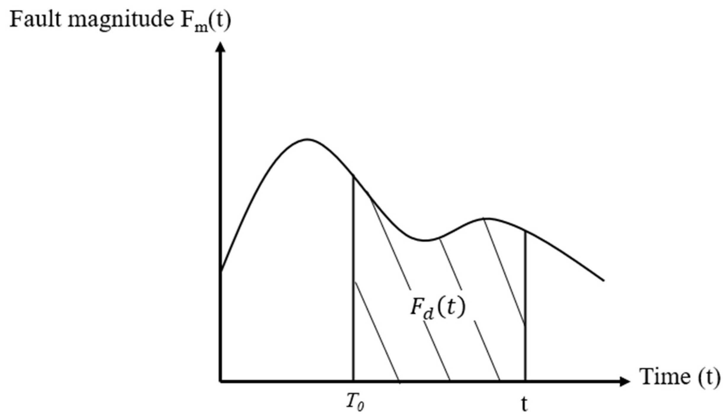
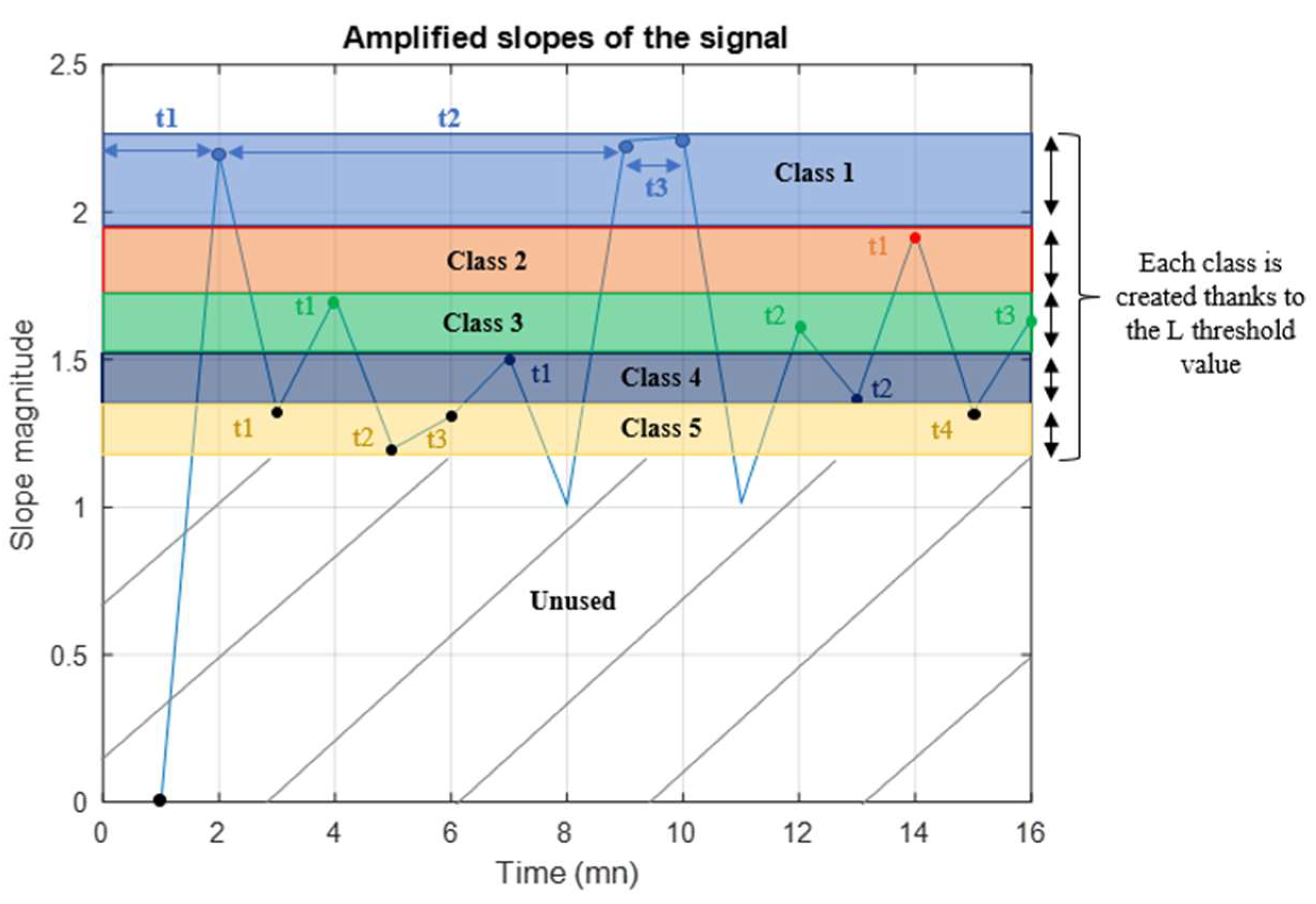
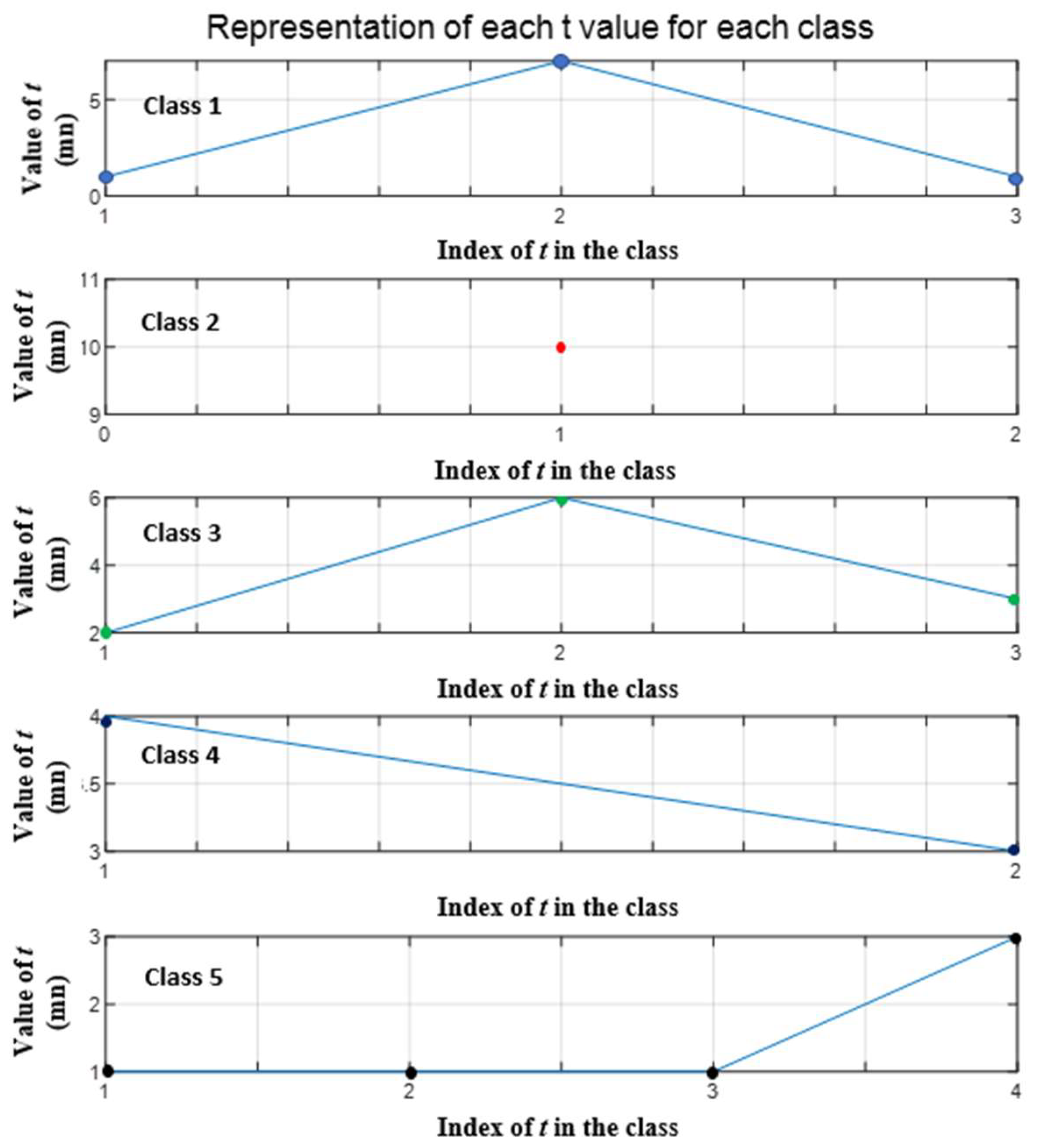
2. Generic Fault Diagnosis Algorithm

The proposed generic fault diagnosis algorithm (GDA) is an online approach. It has been developed for time-domain signals and uses a reduced number of mathematical operations for better implementation in a microcontroller. Other time domain algorithms also exist in the literature as in the case of the Time Domain Averaging (TDA) algorithm. The TDA algorithm manages to improve the information-noise ratio (I/N r) in the signal. For instance, in [11] authors use a TDA algorithm to extract a periodic component from a noisy signal. They explained that the method managed to increase the I/N r of the periodic component in the measured signal and therefore reduces noisy components and amplifies the information. The authors applied an improved TDA algorithm on a nitrogen compressor on which the periodic behavior is easy to determine. They underline that the classic TDA algorithm has an accuracy issue regarding the period which is denoised. Indeed, the cutting period presents a loss of efficiency after the n-cutting period of the signal. Authors, show some attenuation coefficients regarding the classic TDA versus the improved one. The first one shows an attenuation coefficient of 0.711 for the first period and 0.124 for the fourth period. The improved TDA algorithm shows for the first period an attenuation of 0.993 and 0.891 in the fourth one. Shin et al. [12] paper also deals with the TDA algorithm and proposes another method for the I/N r improvement. The authors used a Kalman filter-based TDA (K-TDA) with a periodic signal generated from a computer. They conclude that the two methods produce nearly the same results. However, they pointed out that K-TDA is well applicable to real-time fault diagnosis systems.

The proposed GDA also tries to improve the I/N r of a signal. Indeed, it manages to improve the I/N r of a non-periodic signal, while filtering the wrong diagnosis and giving information about the fault magnitude that occurred in the studied system. The GDA is based on the analysis of the signal components which are considered the distribution of the signal amplitudes. For a better understanding, let us consider a Gaussian random signal U assumed to be a voltage signal as plotted in Figure 3:

The computation of the slopes is set to get the variation of the signal between two periods:

$$\mathrm{S}\left(\mathrm{k}\right)=\frac{\mathrm{U}(\mathrm{k}+1)-\mathrm{U}\left(\mathrm{k}\right)}{{\mathrm{T}}_{\mathrm{sample}}}$$

(2)

where S is the slope of the signal between two samples k, k + 1 and T_sample is the sampling period.

Then, each value of S is amplified or reduced to highlight the information that has to be operated. In this work, the exponential function is chosen to perform this amplification. Indeed, the exponential function allows to amplify high values of S whereas low values stay low:

$$\mathrm{E}\left(\mathrm{k}\right)=exp\left(\right|\mathrm{S}\left(\mathrm{k}\right)\left|\right)$$

(3)

The amplified signal is represented in Figure 4:

Then, each value of E is distributed from the higher to the lower ones into several packages. The created packages are called classes. The number of elements that are put into the classes and the number of classes depends on a threshold value of L.

Figure 5 is an illustration of the class separation.

The L value is assumed to be at 0.099 for the rest of the document. Then, based on the created classes C, the time t_a between each value of E is gathered. This process is explained with the Algorithm 1:

Algorithm 1: class seperation of the signal E

BEGIN

real E, Emax, k, C, n, a, j, index, Tsample, L

n ← 1

Tsample ← 1

L ← 0.099

a ← 0

j ← 0

while length(E) > 0 do

Emax ← max(E)

for k from 1 to length(E) do

if Ek ≥ Emax − (Emax × L)

Ca,j ← (k − n) × Tsample    //The time Ta of the jth class

n ← k

index_k ← k

a ← +1

end

end

E ← suppress (Eindex)

j ← j + 1

end

END

Where k is the index of the element of E, n is the previous gathered time and T_sample is the sampling period of the measured signal. C_a,_j represents t_a^th time value of the j^th class. Each value of C_a,_j is represented in Figure 6. In this example, the proposed procedure leads to five classes. It is worth noting that the number of elements of each class is different.

It is then possible to compute the mean of each representation of t for each class to observe the signal characteristics. Thus, the computation of the average of each class is done by the following equation:

$${\mathrm{M}}_{\mathrm{j}}=\frac{{\sum }_{\mathrm{a}=1}^{\mathrm{a}=\mathrm{n}}{\mathrm{C}}_{\mathrm{a},\mathrm{j}}}{{\mathrm{N}}_{\mathrm{e}}}$$

(4)

where j is the rank of the class, M_j is the average of class j, C_a,j is the value of the j class, and m is the number of elements in class j.

A representation of the average value on a single plot is then possible as shown in Figure 7:

The class average representation is then placed on a fixed number of classes F to always have a fixed number of classes. This number is a GDA parameter. For that purpose, an empty vector V with a higher size than the number of classes of M is created. Each value of M_j is then placed into the V by filling it in by the end. The use of a fixed scale allows for the avoidance of any loss of information and also allows the superposition and comparison of several signals. Finally, the size of V is reduced to get F. To proceed to fault detection and identification, three minimum different sizes of V should be considered. The creation of the reduced vector V to F is depicted in Algorithm 2:

Algorithm 2: representation of the GDA output on a F window

BEGIN

for n from 0 to 2    // Initialisation of V

x = [10, 15, 20];   // 10, 15, and 20 are the three different sizes of V

vector Vn ← zeros(x(n))  // User choice

array M

for i from 0 to length(Vn) do

if i ≤ length(M) do

Vn (length(Vn)-i) = M(length(M)-i)

end

end

vector F ← 10    // The number of desired classes

real nStep = length(Vn) ÷ length(F)

for i from 0 to length(F)

F(i) = Sum (Vn(i*nStep: i*nStep+nStep)) ÷ nStep

end

end

END

The presented algorithm is tested and validated on a DC motor voltage variable, used for a fan application. The purpose of the experiment consists to highlight the ability of the GDA to detect a fault occurrence and to provide fault identification.

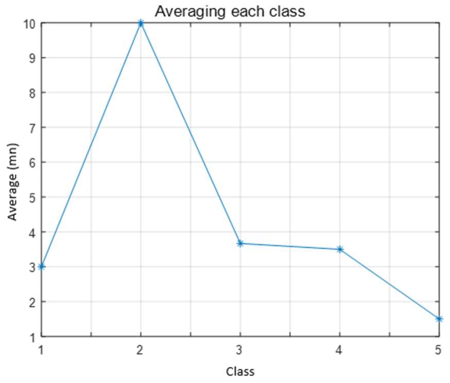
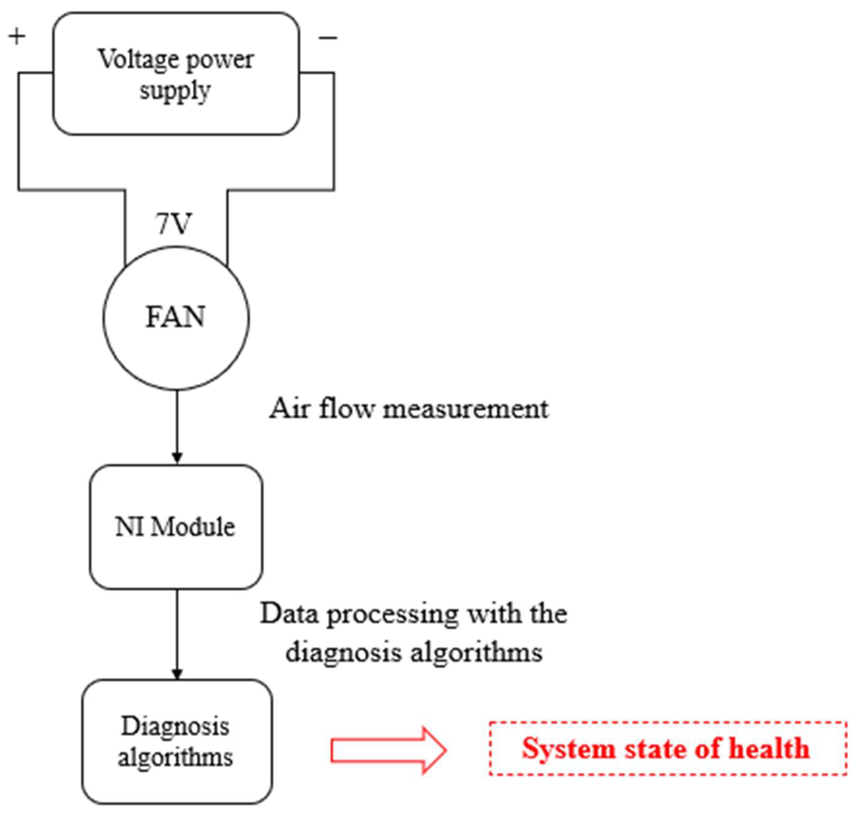
3. Experimental Validation of the GDA Algorithm

In this section, the performance and genericity of the proposed diagnosis tool are experimentally evaluated for two different applications. First, a fan during two faulty operation modes is considered. Second, the diagnosis of a proton exchange membrane fuel cell is evaluated.

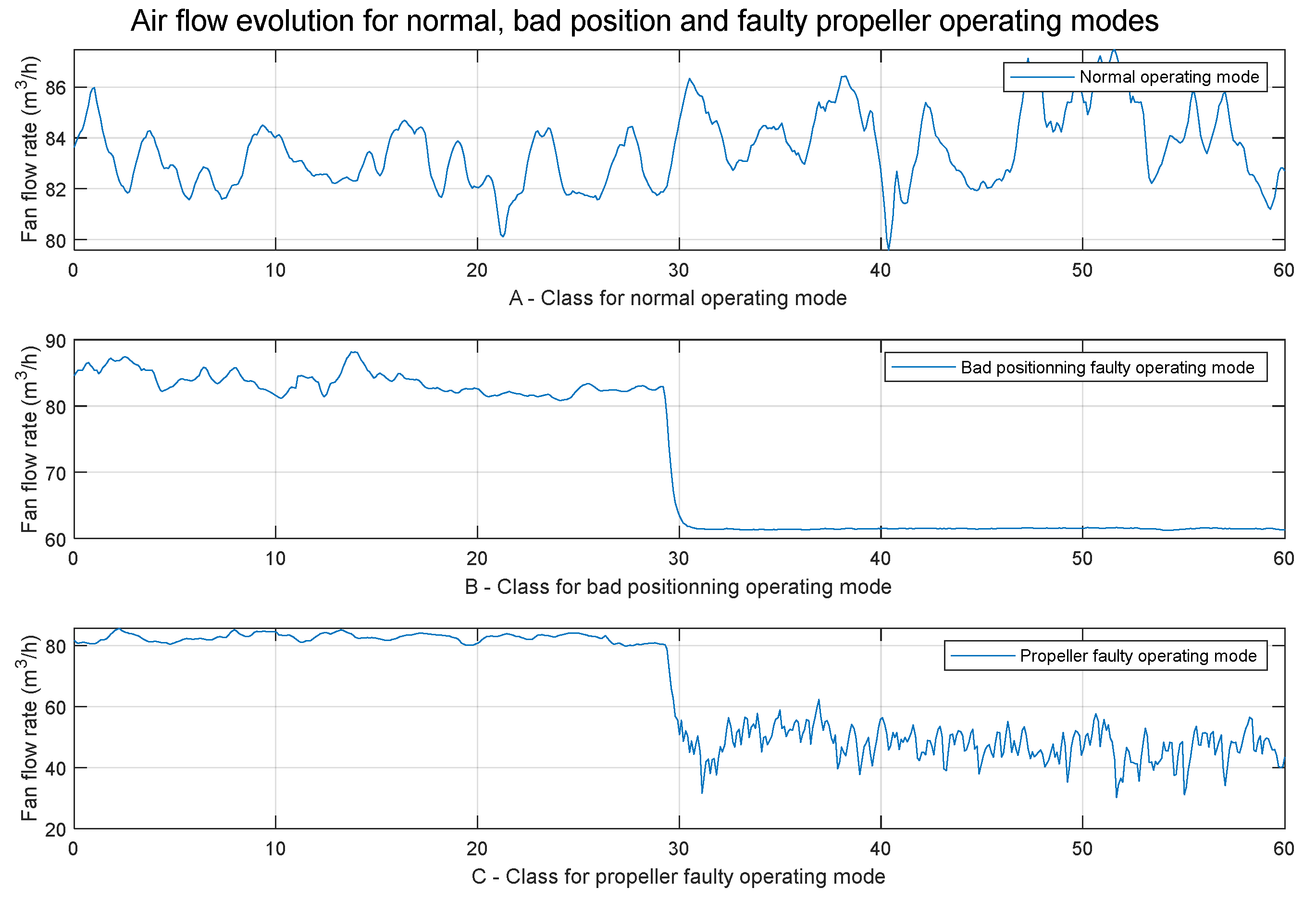
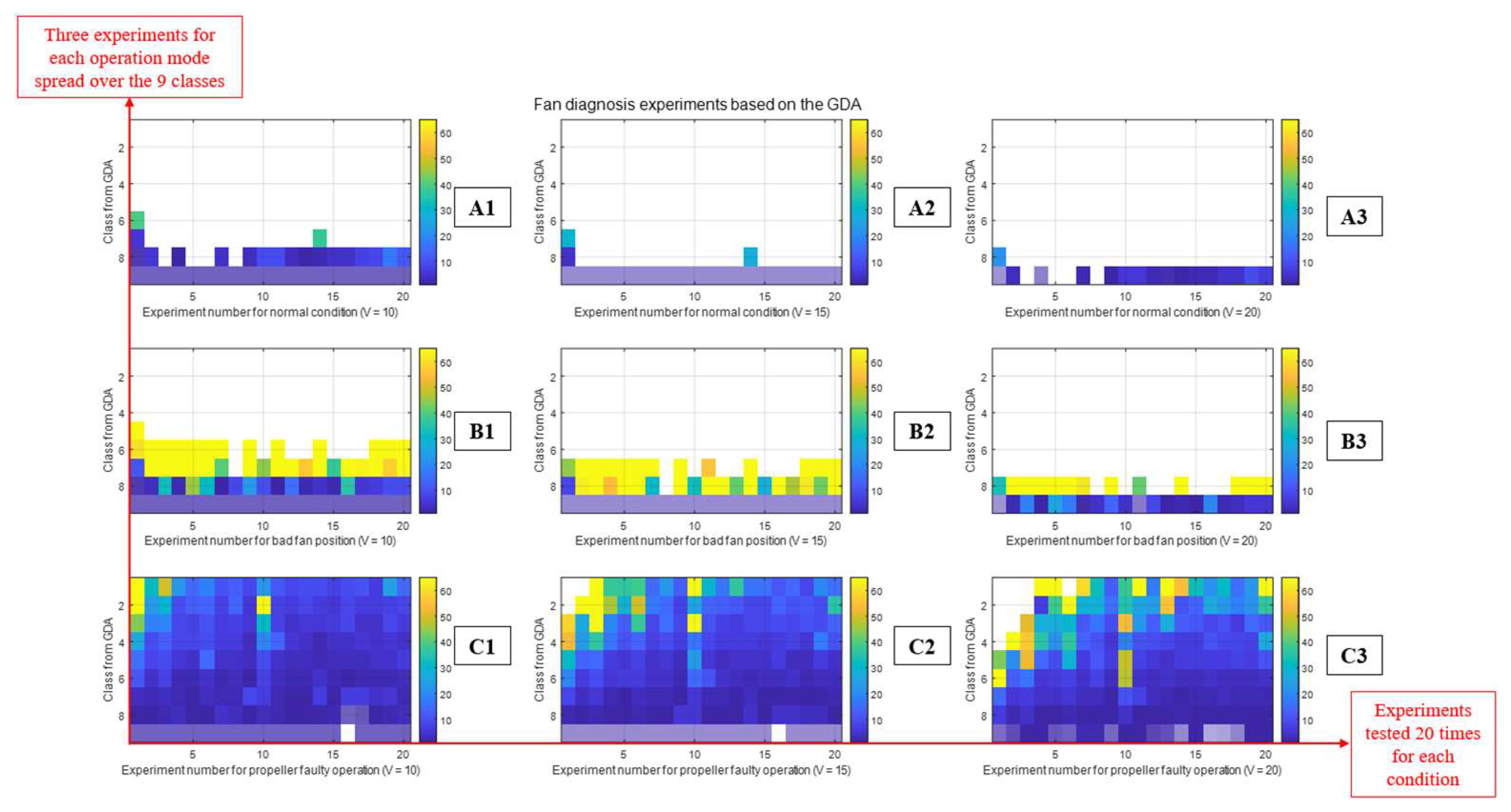
First Application: Application of the GDA to a Fan

The experimental validation is carried out on a fan that operates under three modes: normal condition with a vertical position of the fan; faulty condition with a horizontal position of the fan on a table; faulty condition with finger pressure on the propeller.

The fan has a square dimension with a side of 120 mm. It is 7 V supplied and the maximum air flow is 82.5 m³/h measured thanks to a tachymeter. DC motor voltage information is gathered through a National Instrument module and sent to the diagnosis algorithm. Figure 8 is the assembly diagram that presents the used test bench for the diagnosis algorithm validation.

The next step of the experimental validation consists to set the test protocol. The next section, therefore, proposes the implementation of the experimental protocol.

Experimental protocol for the diagnosis tool

The validation of the GDA is carried out in three cases. The goal is to highlight its ability to observe normal conditions. The ability of the GDA to identify two types of faults is considered. First, the bad positioning faulty condition (fault 1). Secondly, the propeller’s faulty condition (fault 2).

Case 1: the experimental protocol for the normal condition is given below:

• Set the fan vertically on a flat, unobstructed surface,
• Proceed to a 2 Hz air flow measurement,
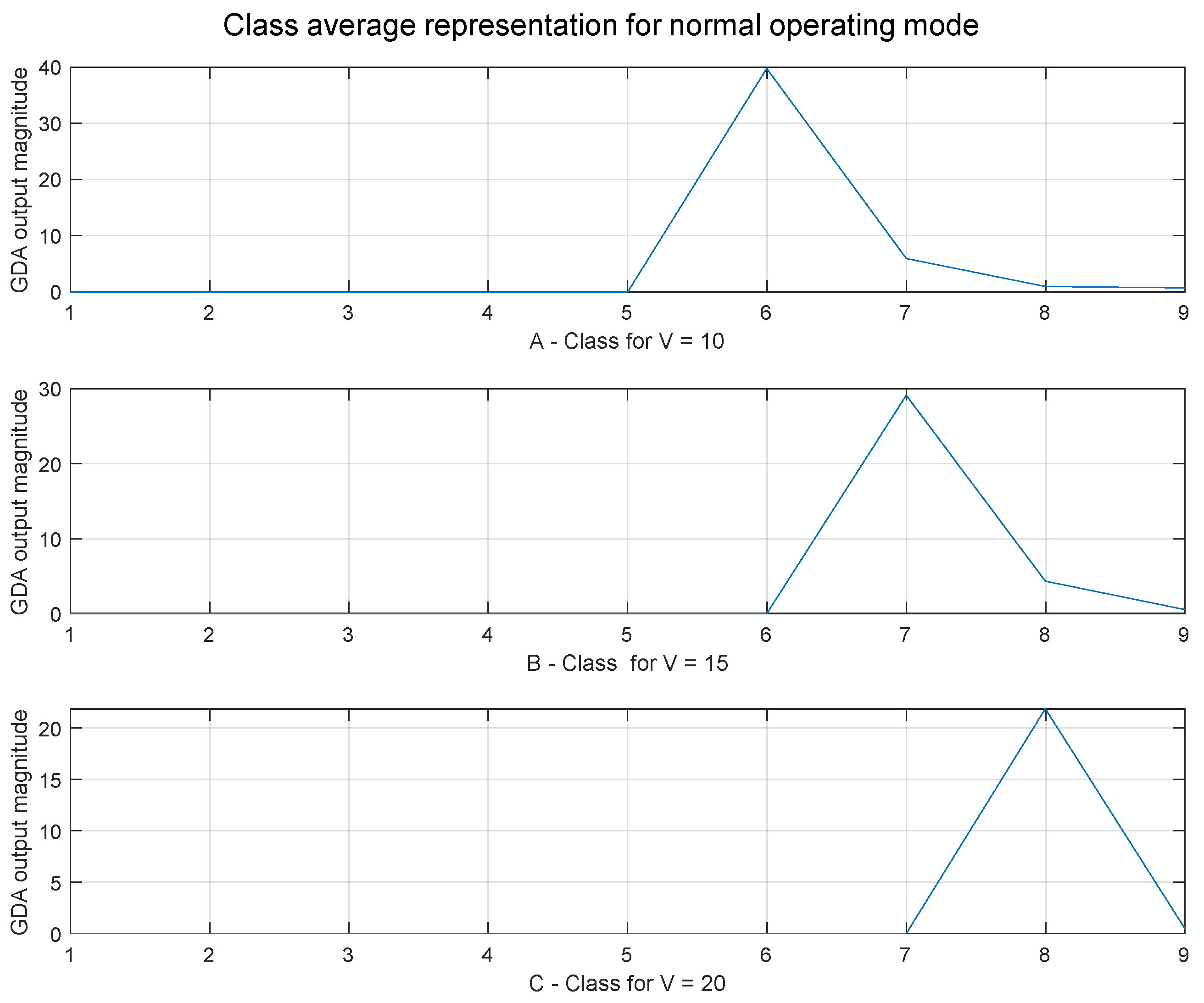
• Compute the normalized representation of the average of each class,
• Compare the result to another normal condition and conclude about the operating mode.

Case 2: the experimental protocol for the bad positioning faulty condition is given below (fault 1):

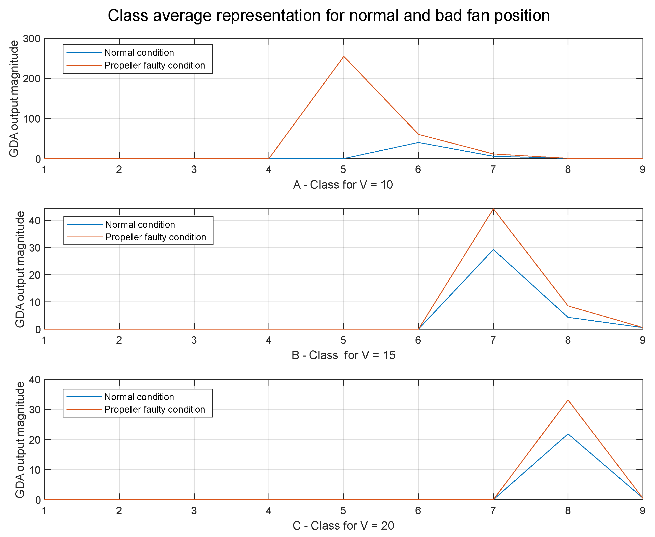
• Set the fan horizontally on a flat surface,
• Proceed to a 2 Hz air flow measurement,
• Compute the normalized representation of the average of each class,
• Compare the result to a normal condition and conclude about the operating mode.

Case 3: the experimental protocol for the propeller’s faulty condition is given below (fault 2):

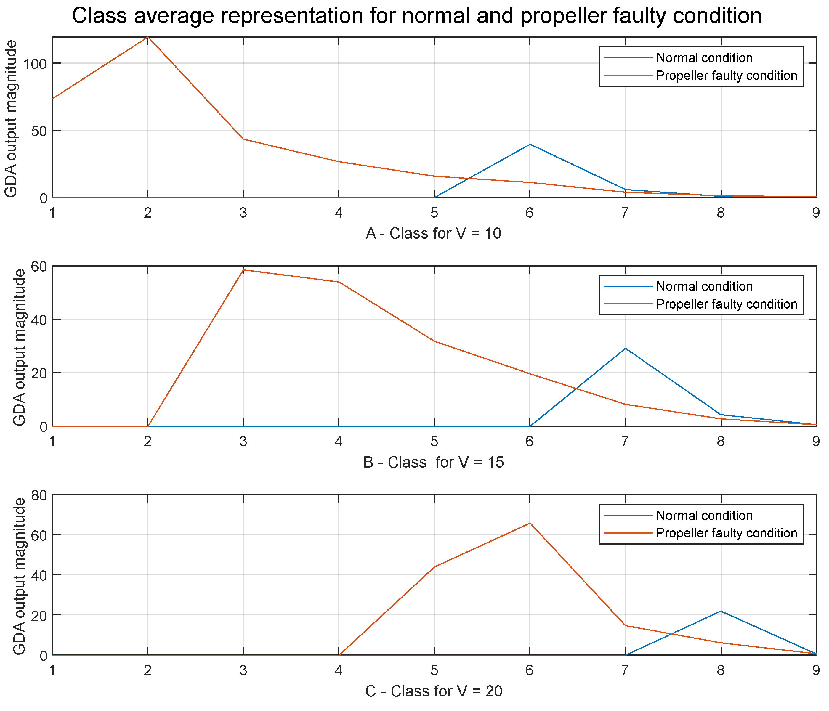
• Set the fan vertically on a flat surface and perform a random pressure on the propeller,
• Proceed to a 2 Hz air flow measurement,
• Compute the normalized representation of the average of each class,
• Compare the result to a normal condition and conclude about the operating mode.

Experimental validation

To characterize the operating conditions of the fan, three measurements are carried out. The first is the measurement of a normal condition, the second is the bad positioning condition and the third is the propeller faulty operating mode. Figure 9 represents these three measurements.

Regarding the B and C graphs in Figure 9, the faulty condition occurs at the 30th second: 0 to 30 s is a normal operating mode and 30 to 60 s are faulty conditions.

Then, each class averaging is represented with the following algorithm configuration:

-

Limit value = 0.62.

-

Tsample = 0.5 s.

-

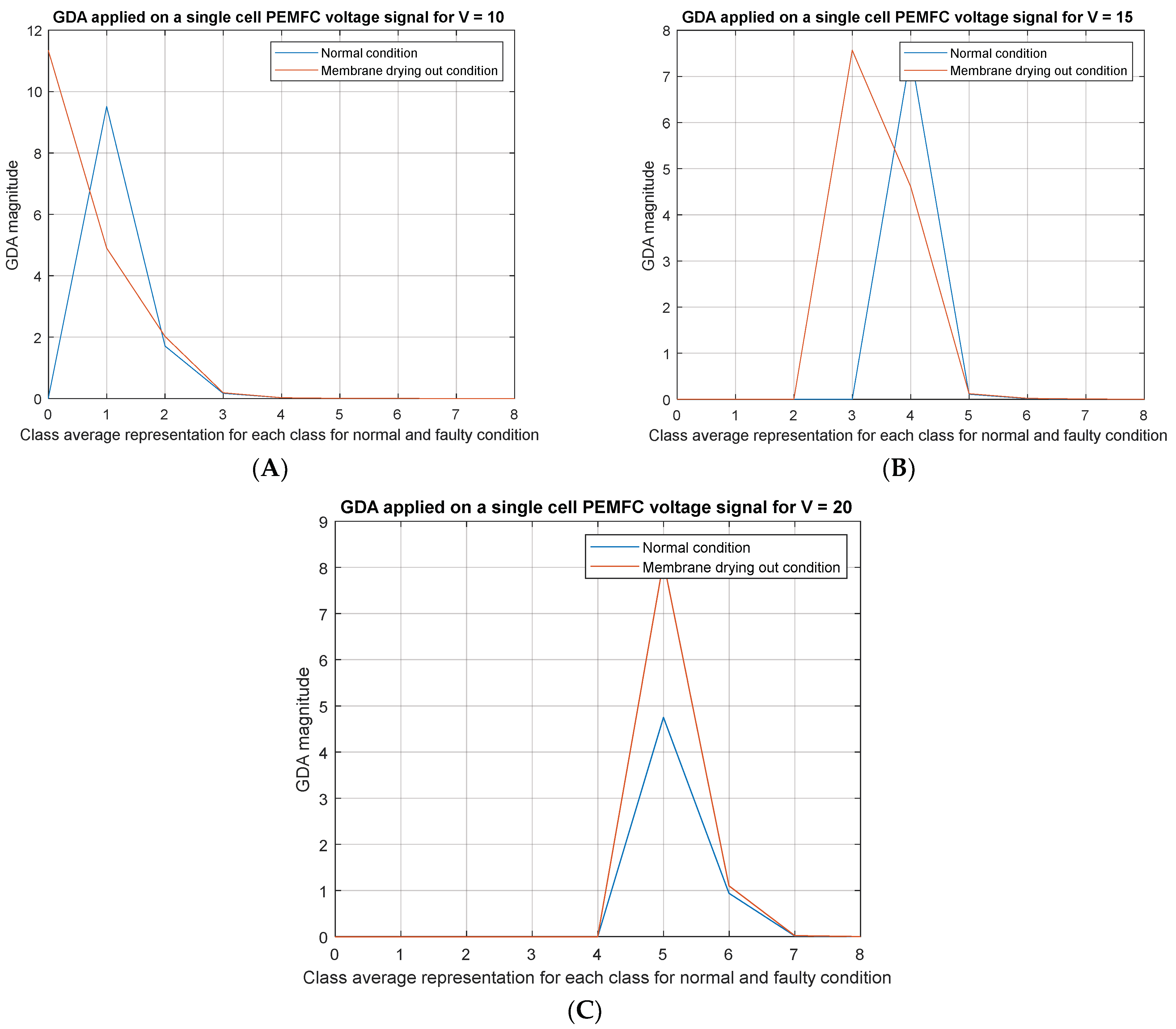
Three values V for the normalization: V1 = 10; V2 = 15; V3 = 20.

-

Representation in 9 classes.

As for Figure 7, the normal fan condition is represented for the three V values in Figure 10:

The next step is now to represent the bad positioning operating mode overlaid on Figure 10 which is considered as the reference for the next steps.

Bad positioning faulty operating condition and characterization (fault 1).

The reference measurement is also kept for comparison with the bad positioning test case. The classes’ average representations are plotted in Figure 11:

Figure 11 shows a modification of the faulty class value (red curve) and exceeds the reference values of the normal condition (blue curve). That means that a bad position faulty condition has been pointed out by the GDA.

Propeller faulty operating condition and characterization (fault 2).

As for previous tests cases, the normal measurement is kept as a reference for a good comparison with another propeller’s faulty condition in Figure 12:

Figure 12 shows a modification of the faulty class value (red curve) and exceeds the reference values of the normal condition (blue curve). That means that the propeller’s faulty condition has been pointed out by the GDA.

Each case (normal condition, fault 1, fault 2) is repeated 20 times, and the GDA is applied for 3 different values of V (V = 10, V = 15 and V = 20). The results are presented for 9 classes in Figure 13.

Figure 13 shows the three fan operating modes which are repeated 20 times. The test number which has been carried out is represented on the horizontal axis. The vertical axis is the normalized class representation of the GDA.

A1, A2 and A3 are the normal fan operating modes. The white color corresponds to an empty class whereas the colored cases correspond to the class values with blue for low and yellow for high values. The comparison between B1 to B3 shows that there are fewer white cases distributed in each class. This is due to the fault occurrence which creates new values on the GDA classes. This is the same interpretation between Bx experiments and C1 to C3 where more class values are generated by the propeller faulty operated mode. Therefore, it is possible to detect a fault occurrence regarding the distribution of the class values. The experiments also show several kinds of distributions between the operating modes. That difference allows the identification of the current operating mode:

-

A low number of classes with low values is equivalent to a normal operating mode,

-

A low number of classes with high values is equivalent to the occurrence of bad fan positioning,

-

A high number of classes with a mix of low and high values is equivalent to the occurrence of a propeller faulty operation.

Based on these observations the following rule-based diagnosis is considered in the Algorithm 3:

Algorithm 3: rules for diagnosis

BEGIN           //Example for V = 10

Integer nClass_normal = 2   // Number of maximum classes for a normal condition

Integer Value_Normal_Classe2 = 15 // Highest value of the second class for normal condition

vector flag1, flag2 = 0;    // Flags for fault detection

char status = “normal”;

for i from 0 to 8

vector M = [1:9]  // Value of each class M

if Mi > 0 do

flag1_i = 1; // To compute the number of non-empty classes

end

if Mi > Value_Normal_Classe2 do

flag2_i = 1; //To check if a class value is higher than the normal class

end

end

if SUM(flag1) > nClass_normal AND SUM(flag2) ! = 0 do

status = “fault”;

end

END

The GDA performance can also be evaluated with four metrics:

-

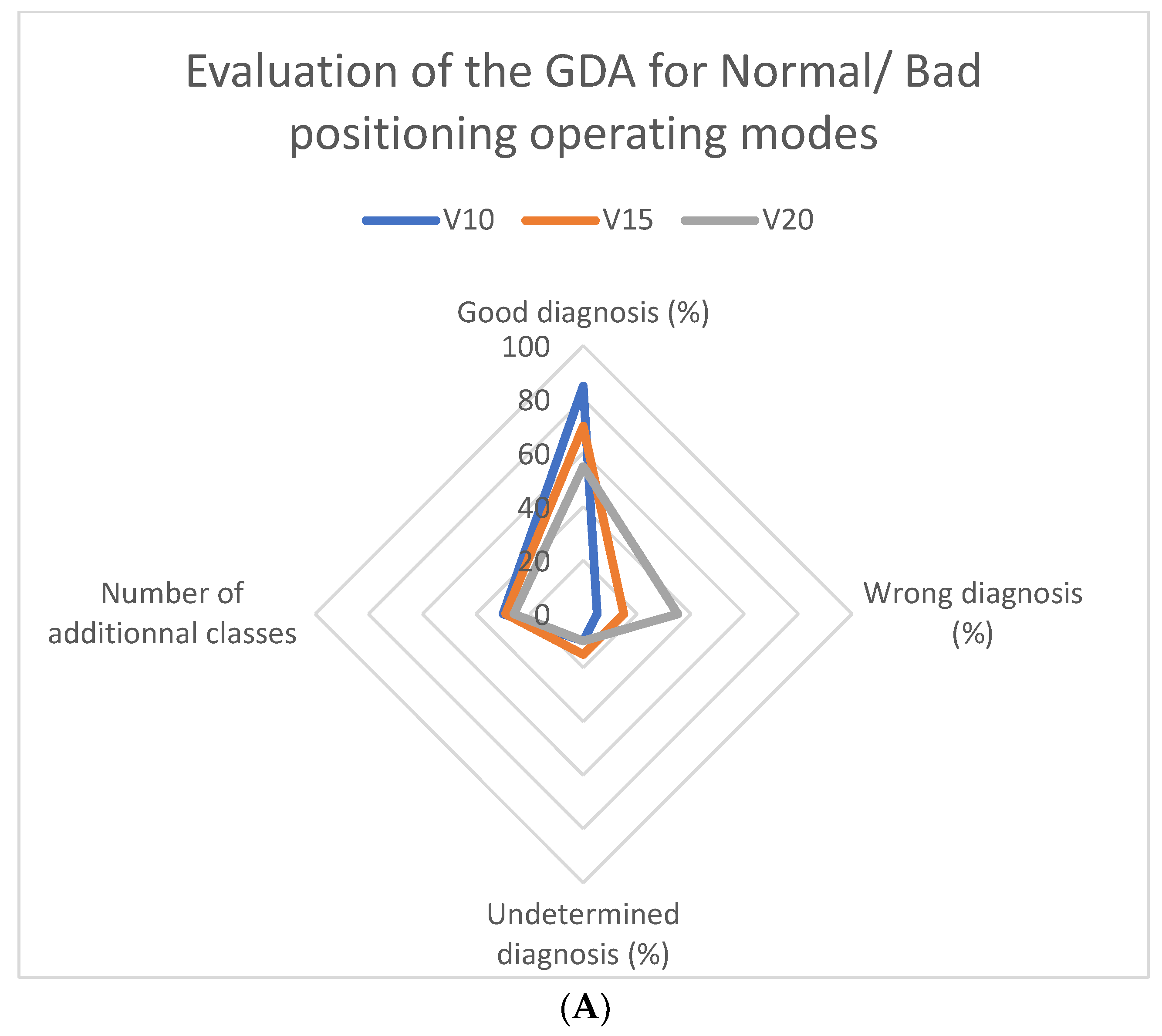
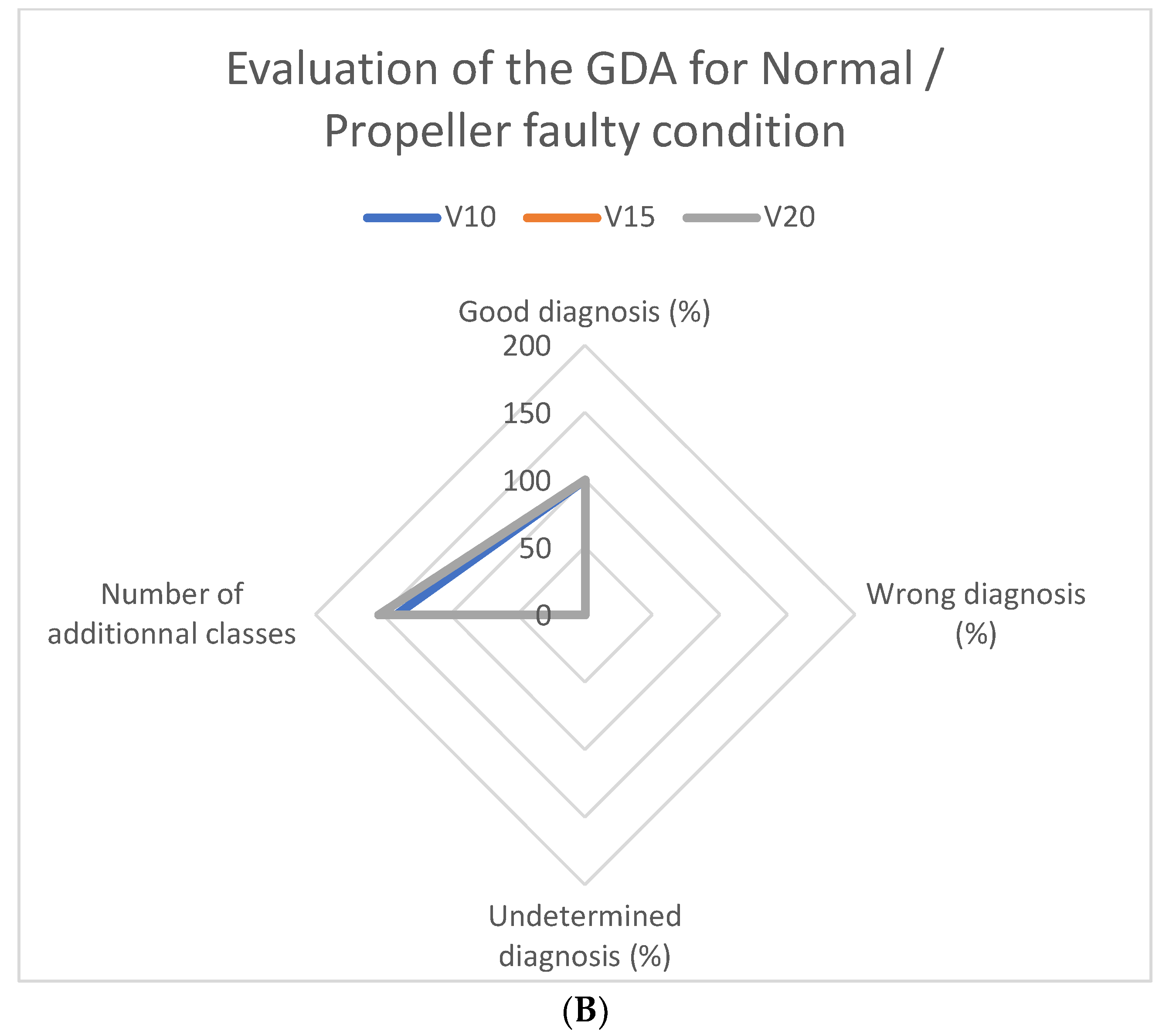
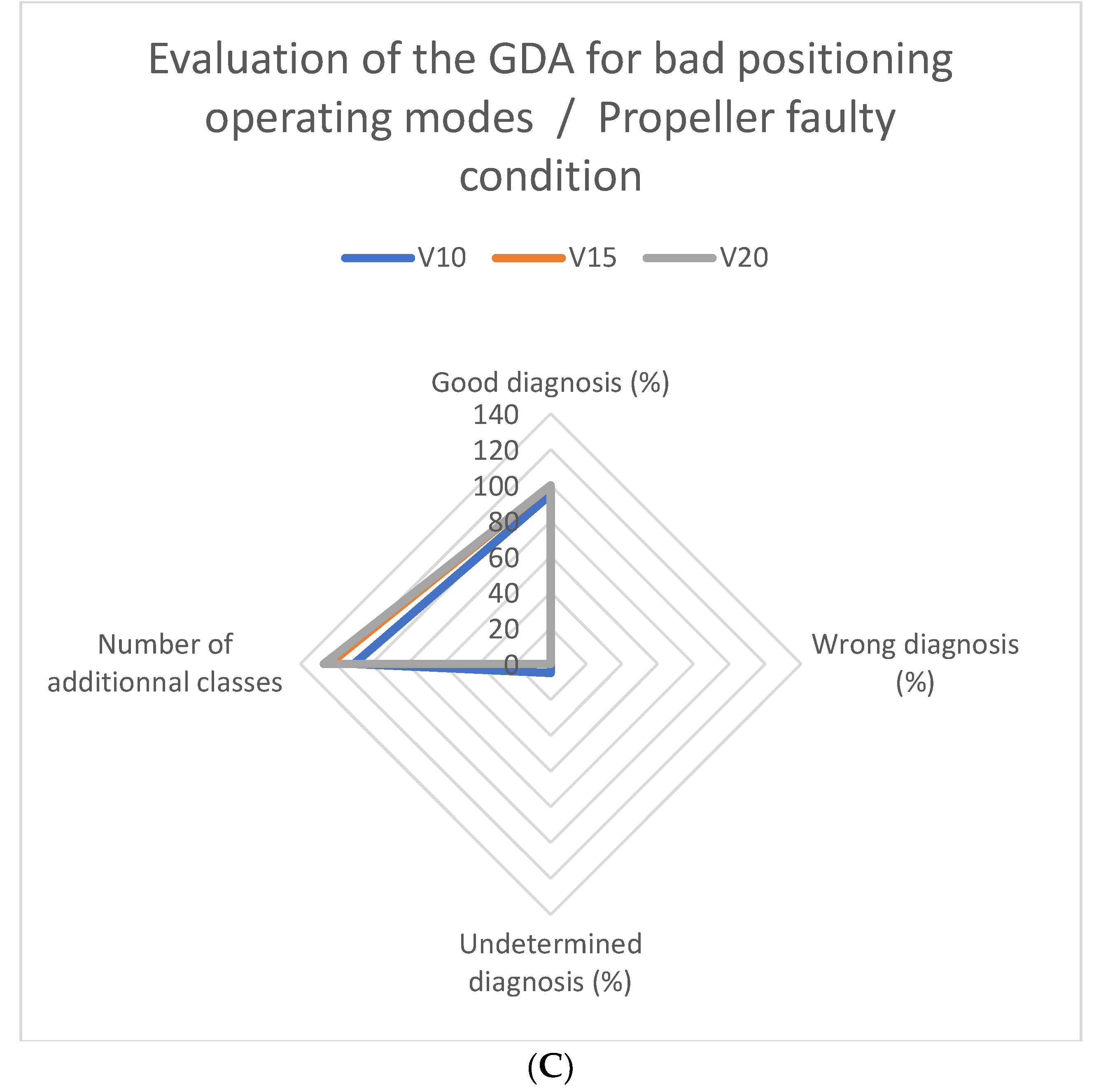
Number of good diagnoses,

-

Number of wrong diagnoses,

-

Undetermined operating mode,

-

Number of additional classes.

Based on the defined metrics, the GDA for normal with bad positioning modes, normal with propeller faulty mode, and bad positioning with propeller faulty mode are evaluated in Figure 14:

Figure 13 shows the ability of the GDA to diagnose without wrong diagnosis a propeller faulty condition. However, its ability to correctly detect and identify a bad fan positioning depends on the value of V. Indeed, there is 85% of good fault detection and 5% of wrong detection. The remaining 10% are undetermined system operating modes.

The genericity of the GDA is related to its ability to be applied to several other systems. For instance, an application on a single-cell fuel cell system has been carried out for two operating modes which are assumed to be normal and in a faulty condition. This application is depicted in the next section.

Second application: Application of the GDA to a single-cell fuel cell.

The validation of the GDA proceeded on a single-cell proton exchange membrane fuel cell (PEMFC) on a test bench on an FCT brand [9]. The used fuel cell is supplied with pure hydrogen and oxygen for maximum power production of 50 W. The membrane electrolyte assembly (MEA) has 50 cm² of active area with 0.5 mg/cm² of platinum.

The experiment consists of observing a normal operating condition versus a faulty condition of a fuel cell through the GDA. The normal operating condition consists to place the setpoint near 0.7 V and carrying out the fuel cell voltage for 1 min at 1 kHz. The faulty condition is the membrane drying out as depicted in [10,11,12] and consists to evacuate the membrane water content from the fuel. The membrane drying-out protocol is based on a previous study [13] where the input gases are dry and the flow rate is increased to evacuate as more of possible the fuel cell water. The voltage is then carried out for 1 min at 1 kHz. The measurements are displayed in Figure 15.

The operating condition is shown in the following

Table 1. Setting for normal and drying out conditions.

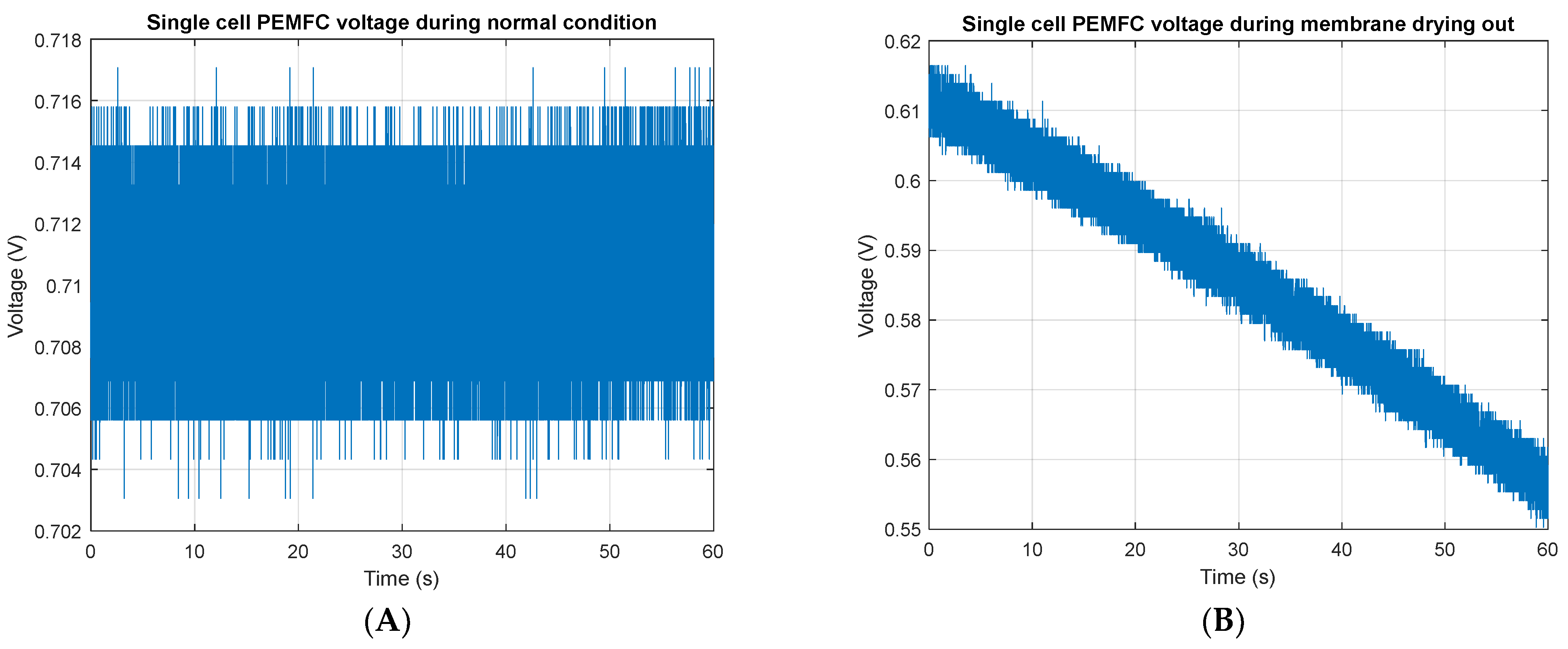
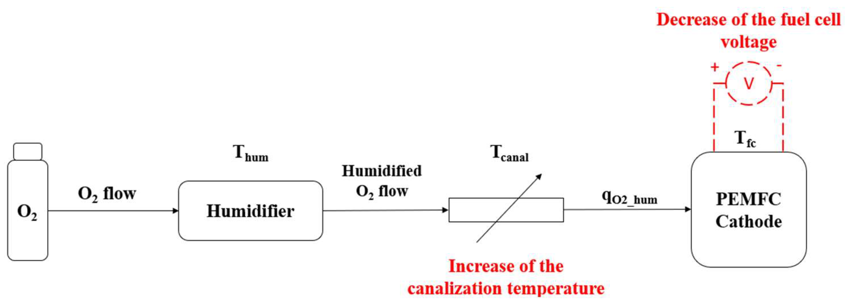
	Normal Operating Conditions	Drying out Operating Condition
Ifc (A)	20 (0.4 A cm−2)	20 (0.4 A cm−2)
λH2 (stoichiometry)	2.5	2.5
λO2 (stoichiometry)	3	10
Tfc (°C)	70	70
Tcanal (°C)	70	70
Thum (°C)	62	55
Relative humidity (%)	70	50

:

Where I_fc is the fuel cell current, λ_H2/O2 are the hydrogen and oxygen stoichiometries, T_fc is the fuel cell temperature, T_canal is the supply canalization temperature, T_hum is the humidification temperature.

Figure 16 shows each auxiliary used on the fuel cell cathode feeding line. Indeed, the dry oxygen crosses the humidifier and springs from it at 100% of relative humidity. T_canal is finely tuned to reduce the water content of the wet gas from 100% to 50%. In this way, the membrane water content decreases which implies a fuel cell voltage decrease.

Figure 17 shows three GDA outputs for the considered values of V. Results show that faulty conditions can be observed on all GDA representations. Regarding V = 10, a new value appears in class 0 (C0). It is the same observation for V = 15 for class 3 (C3). Regarding V = 20, it is an incrementation of the existing class values of C5, C6 and C7 which happen on the output of the GDA. As for V = 20, all classes are incremented it is possible to consider this representation for the single-cell fuel cell membrane drying out characterization.

The experimental tests of the GDA on a single-cell PEMFC thus show the genericity of the approach. Nevertheless, more fuel cell experiments should be done to highlight the algorithm’s ability to identify the fault occurrence and more, the fault degree.

Note that, due to the amount of data used for the GDA process and the chosen limit, some low components are not observable. For that reason, a better data window should be found and a dynamic limit would be relevant for a more detailed analysis of the signal.

4. Conclusions and Discussion

The paper proposed a novel time-domain fault diagnosis algorithm suitable for fast implementation in a microcontroller. Faults manage to be detected and identified with low computational time. The major strength of the method is its ability to avoid wrong measurement or fugitive phenomena and therefore prevent wrong fault diagnosis. The novel fault detection and isolation proposed in this paper is a complementary approach to the offline designs in the literature as depicted in the introduction. The developed method is an online approach that manages the observation of abnormal conditions that would not be taken into consideration by offline considerations. The performance and the genericity of the novel proposed approach have been experimentally evaluated on a fan considering two different faulty conditions and on a proton exchange membrane fuel cell. The experimental results have demonstrated the high efficiency of the proposed diagnosis tool.

Regarding the first application, the three test cases show that GDA manages to detect normal and faulty conditions. However, if a focus is given to the class values, it is possible to identify the faulty condition. Indeed, regarding Figure 10 and Figure 11 it appears that each faulty condition generates some new classes at the GDA output. The interpretation of these new values can be found inside the input signal. In fact, since the GDA analyses the slopes in the signal, the new class apparition means that there is agitation due to the faulty condition. For instance, if a comparison is made between Figure 10 and Figure 11 each faulty condition affects different class values.

Regarding the second application, two operating modes are characterized by the GDA: normal and membrane drying-out modes. For both signals, classes are extracted by the GDA and plotted in Figure 16. There are additional classes of apparitions during a faulty condition due to some new excitations. Moreover, the magnitude of the classes is also amplified in the case of V = 20. The GDA, therefore, manages to detect new behavior in the fuel cell voltage that allows the detection of another operating condition. The validation of the GDA approach should be carried out on a fuel cell stack which is the purpose of the next work.

Therefore, the GDA manages to distinguish a faulty condition from a normal condition. It also can detect and identify the fault nature by observing each class value. However, it has not been possible to characterize the fault magnitude. Further work would be necessary to determine this parameter.

Indeed, it manages to detect and identify a fault occurrence according to the environment where the system operates. Moreover, the wrong diagnosis is drastically reduced and allows a reliable interpretation of the operating conditions. To illustrate its genericity, the algorithm has been applied to a fan and a fuel cell, obviously it could be applied to other systems, which is the purpose of further work.

References

- Dijoux, E.; Steiner, N.Y.; Benne, M.; Péra, M.-C.; Pérez, B.G. A review of fault tolerant control strategies applied to proton exchange membrane fuel cell systems. J. Power Sources 2017, 359, 119–133. [Google Scholar] [CrossRef] [Green Version]
- Yang, C.; Gui, W.; Chen, Z.; Zhang, J.; Peng, T.; Yang, C.; Karimi, H.R.; Ding, S.X. Voltage Difference Residual-Based Open-Circuit Fault Diagnosis Approach for Three-Level Converters in Electric Traction Systems. IEEE Trans. Power Electron. 2020, 35, 3012–3028. [Google Scholar] [CrossRef]
- Steiner, N.Y.; Hissel, D.; Moçotéguy, P.; Candusso, D.; Marra, D.; Pianese, C.; Sorrentino, M. Application of Fault Tree Analysis to Fuel Cell diagnosis. Fuel Cells 2012, 12, 302–309. [Google Scholar] [CrossRef]
- Dijoux, E.; Steiner, N.Y.; Benne, M.; Péra, M.-C.; Grondin-Perez, B. Fault Structural Analysis Applied to Proton Exchange Membrane Fuel Cell Water Management Issues. Electrochem 2021, 2, 38. [Google Scholar] [CrossRef]
- Li, G.; Yao, Q.; Fan, C.; Zhou, C.; Wu, G.; Zhou, Z.; Fang, X. An explainable one-dimensional convolutional neural networks based fault diagnosis method for building heating, ventilation and air conditioning systems. Build. Environ. 2021, 203, 108057. [Google Scholar] [CrossRef]
- Bouzida, A.; Touhami, O.; Ibtiouen, R.; Belouchrani, A.; Fadel, M.; Rezzoug, A. Fault Diagnosis in Industrial Induction Machines through Discrete Wavelet Transform. IEEE Trans. Ind. Electron. 2010, 58, 4385–4395. [Google Scholar] [CrossRef]
- BahooToroody, F.; Khalaj, S.; Leoni, L.; De Carlo, F.; Di Bona, G.; Forcina, A. Reliability Estimation of Reinforced Slopes to Prioritize Maintenance Actions. Int. J. Environ. Res. Public Health 2021, 18, 373. [Google Scholar] [CrossRef] [PubMed]
- Kumar, A.; Kumar, V.; Modgil, V. Behavioral study and availability optimization of a multi-state repairable system with hot redundancy. Int. J. Qual. Reliab. Manag. 2019, 36, 314–330. [Google Scholar] [CrossRef]
- Velmurugan, K.; Saravanasankar, S.; Venkumar, P.; Sudhakarapandian, R.; di Bona, G. Availability Analysis of the Critical Production System in SMEs Using the Markov Decision Model. Math. Probl. Eng. 2022, 2022, 026984. [Google Scholar]
- Kitsios, F.; Chatzidimitriou, E.; Kamariotou, M. Developing a Risk Analysis Strategy Framework for Impact Assessment in Information Security Management Systems: A Case Study in IT Consulting Industry. Sustainability 2022, 14, 1269. [Google Scholar] [CrossRef]
- Liu, H.; Zuo, H.; Jiang, C.; Qu, L. An improved algorithm for direct time-domain averaging. Mech. Syst. Signal Process. 2000, 14, 279–285. [Google Scholar]
- Shin, K. Realization of the real-time time domain averaging method using the Kalman filter. Int. J. Precis. Eng. Manuf. 2011, 12, 413–418. [Google Scholar] [CrossRef]
- Dijoux, E.; Steiner, N.Y.; Benne, M.; Péra, M.-C.; Grondin-Perez, B. Experimental Validation of an Active Fault Tolerant Control Strategy Applied to a Proton Exchange Membrane Fuel Cell. Electrochem 2022, 3, 42. [Google Scholar] [CrossRef]