
Torch-NILM: An Effective Deep Learning Toolkit for Non-Intrusive Load Monitoring in Pytorch


School of Informatics, Aristotle University of Thessaloniki, 54124 Thesssaloniki, Greece
*
Author to whom correspondence should be addressed.
Energies 2022, 15(7), 2647; https://doi.org/10.3390/en15072647
Submission received: 10 February 2022
/
Revised: 16 March 2022
/
Accepted: 30 March 2022
/
Published: 4 April 2022
(This article belongs to the Special Issue Digital Transformation in the Energy Sector: Data-Driven Analytics, Services and Business Models)
Abstract
:Non-intrusive load monitoring is a blind source separation task that has been attracting significant interest from researchers working in the field of energy informatics. However, despite the considerable progress, there are a very limited number of tools and libraries dedicated to the problem of energy disaggregation. Herein, we report the development of a novel open-source framework named Torch-NILM in order to help researchers and engineers take advantage of the benefits of Pytorch. The aim of this research is to tackle the comparability and reproducibility issues often reported in NILM research by standardising the experimental setup, while providing solid baseline models by writing only a few lines of code. Torch-NILM offers a suite of tools particularly useful for training deep neural networks in the task of energy disaggregation. The basic features include: (i) easy-to-use APIs for running new experiments, (ii) a benchmark framework for evaluation, (iii) the implementation of popular architectures, (iv) custom data loaders for efficient training and (v) automated generation of reports.
1. Introduction
Energy management of households is a non-trivial and important task both to the users and the environment [1,2]. A viable, efficient and low-cost solution towards effective energy management [1] is non-intrusive load monitoring (NILM) [3]. The purpose of NILM is to estimate the appliance-level energy consumption given the total energy consumption of a household, using only one active power mains meter. Following the continuous advances of deep learning, most NILM research focuses on developing deep-learning solutions and artificial neural networks to tackle this blind source separation problem.
The two main software tools when conducting deep-learning-based experiments include an efficient data loader that effectively handles any preprocessing steps and a computational framework for rapid model development. The most known and effective data toolkit for loading and preprocessing publicly available NILM datasets is NILMTK [4]. NILMTK is a Python [5] toolkit based on popular data science libraries [6,7]. Most NILM experiments have thus far been implemented using NILMTK in conjunction with machine-learning libraries such as scikit [8], Tensorflow [9], Keras [10] etc.
An alternate very popular framework among researchers is Pytorch [11,12]. This work aims to introduce a pytorch-based library to NILM research that exploits the benefits of this framework. After the introduction of Pytorch Lightning [12] in the Pytorch ecosystem, the workflow is far more user friendly. In addition, debugging is performed with python debuggers. Finally, Pytorch offers built-in extendable objects which can be used to load and preprocess the data more efficiently.
In this research, we introduce Torch-NILM, the first Pytorch-based toolkit for NILM. This toolkit can be used to design, test and benchmark deep learning architectures in the problem of NILM in an efficient and clean way, writing only a few lines of code. The usual problem that NILM researchers face is that there is not a standardised way of composing and executing reproducible experiments. Thus, each researcher ends up developing their own way of conducting NILM experiments. Without an experiment norm, reading and understanding other people’s code may be stressful and inconvenient. In comparison to computer vision or other classic deep learning problems, NILM is becoming harder to start. On top of that, another possible barrier towards reproducible results is the lack of a clear benchmarking methodology alongside specific training and testing data.
Torch-NILM contains six known NILM models, two different deep learning training techniques, a benchmarking framework with four kinds of generalization tests, three popular preprocessing methods used in NILM, three experiment APIs and an automated reporting process with comparative plots. In addition, Torch-NILM is compatible with NILMTK; in fact, it uses NILMTK as a bridge to load the desired measurements into the customised dataset objects, where preprocessing is executed. This paper contributes to the NILM-related research in the following ways. Firstly, it provides a complete NILM-specific Python toolkit based on Pytorch and compatible with the old-time favourite NILMTK in order to produce huge amounts of experiments and results effortlessly, with minimum coding from the user. Secondly, it offers a structured and clean way of creating reproducible and easy-to-read NILM experiments. Thirdly, it provides a set of easily modified, well-known NILM deep learning architectures developed in Pytorch. These models could be used as a guide by researchers when designing their own architectures. Finally, it provides a complete set of specific energy data for training and testing, containing enough end-uses for proper disaggregation. These data are used alongside the benchmark framework described in [13], which contains four different categories of training and testing scenarios.
2. Related Work
The objective of blind source separation research is to extract individual signal sources from the main signal [14]. Non-intrusive load monitoring is essentially a type of blind source separation problem where the goal is to estimate the individual appliance active power consumption using only the total consumption of a household. The term “non-intrusive” refers to the fact that only one meter is used for gathering the measurements of the total house consumption. It is worth noting that even though NILM research focuses on energy estimation, it is a different problem from energy forecasting or prediction [15,16,17].
With the rise of deep learning in the mid 2010s, researchers started to develop NILM applications with neural networks. The work of Kelly and Knottenbelt [18] showed great results and triggered the use of neural networks. Soon, deep learning achieved state-of-the-art results [19,20,21,22] and seems to be the go-to solution for NILM.
In NILM literature, data measurements are provided in a low or high sampling frequency. Low sampling means that measurements are produced at frequencies of 1 Hz and lower. High-frequency measurements are sampled at frequencies in the range of 1 kHz. The majority of NILM research designs algorithms and methods using low-frequency data, due to the fact that most of the smart meters draw measurements in low frequencies. Thus, the majority of the publicly available data sets have been recorded at low frequency [23].
Two machine learning approaches are commonly used to tackle NILM; regression and multi-label classification. In regression approach, the power consumption of a single appliance is estimated [24,25,26,27,28]. Thus, one model per device is created. In multi-label classification approach, the model identifies operating states of various devices. Hence, one model learns to disaggregate a set of devices. Recently published research showed that a multi-label approach achieves good results [29,30,31].
Compared to other classic machine learning problems, NILM has the disadvantage that there are not many domain-specific libraries. NILMTK [4] was introduced in 2014 in order to fill the gap. The main purpose of NILMTK was to help researchers build reproducible results. NILMTK provides data parsers for almost all publicly available datasets alongside baseline models to compare with. Even though NILM data sets usually consume many gigabytes of ROM, NILMTK uses a very efficient format to store all the information. In addition, it provides many built-in functionalities to extract useful energy data statistics. The code is maintainable and often updated by the owners and the NILM community, providing it with new data parsers and architectures. Hence, NILMTK is rightfully established as the standard solution for conducting NILM research. Although this library has been used by the majority of related researchers over the years, it does not provide a standard benchmarking methodology. Moreover, in order to develop and execute experiments, a great amount of coding is necessary.
In an attempt to overcome these barriers and make the library more user friendly, in 2019 some well-known NILM researchers contributed in developing an updated NILMTK API [32] with a cleaner data flow. Two key points of merit can be derived. At first glance, the data preprocessing, architecture, training process and inference are all tangled up in a single “disaggregator” class. Therefore, any changes demand a deep understanding of each “disaggregator” object. Furthermore, even though comparison of algorithms is easier and demands less code writing, a standard set of experiments serving as a benchmark is not provided. This makes data investigation necessary to specify which data sets can be used, which households to choose and which time periods contain proper measurements for training and testing. Moreover, simple performance comparisons between models cannot provide reliable metrics regarding their performance.
Torch-NILM is composed of simple decoupled components; the model, the data handling, the training and the inference are separate processes. Thus, any modification of a process could be performed easily without relying on code deciphering. In addition, the proposed toolkit encapsulates the benchmark developed by Symeonidis et al. [13], which includes multiple types of tests for evaluating model performance in various scenarios. With the underlying use of NILMTK to parse the necessary data for each situation, Torch-NILM is a novel approach to conduct clean, modifiable and reproducible experiments. It should be noted that currently, Torch-NILM supports only regression approaches where one model per device is required. It is available at https://github.com/Virtsionis/torch-nilm, accessed on 10 February 2022.
3. Architecture of Torch-NILM
The proposed toolkit consists of the following key components, organised in separate modules:
- The datasources module is responsible for loading and preprocessing the data.
- The lab module contains the NILM trainer, the deep learning training tools and the APIs to build new experiments.
- In the neural networks module, all the baseline deep learning architectures are located.
- Module utils consists of the reporting processes, the metrics and some helper functions.
- The benchmark module contains the appropriate configuration files for all categories of experiments. Each file contains the selected datasets, households and dates needed for the corresponding experiment.
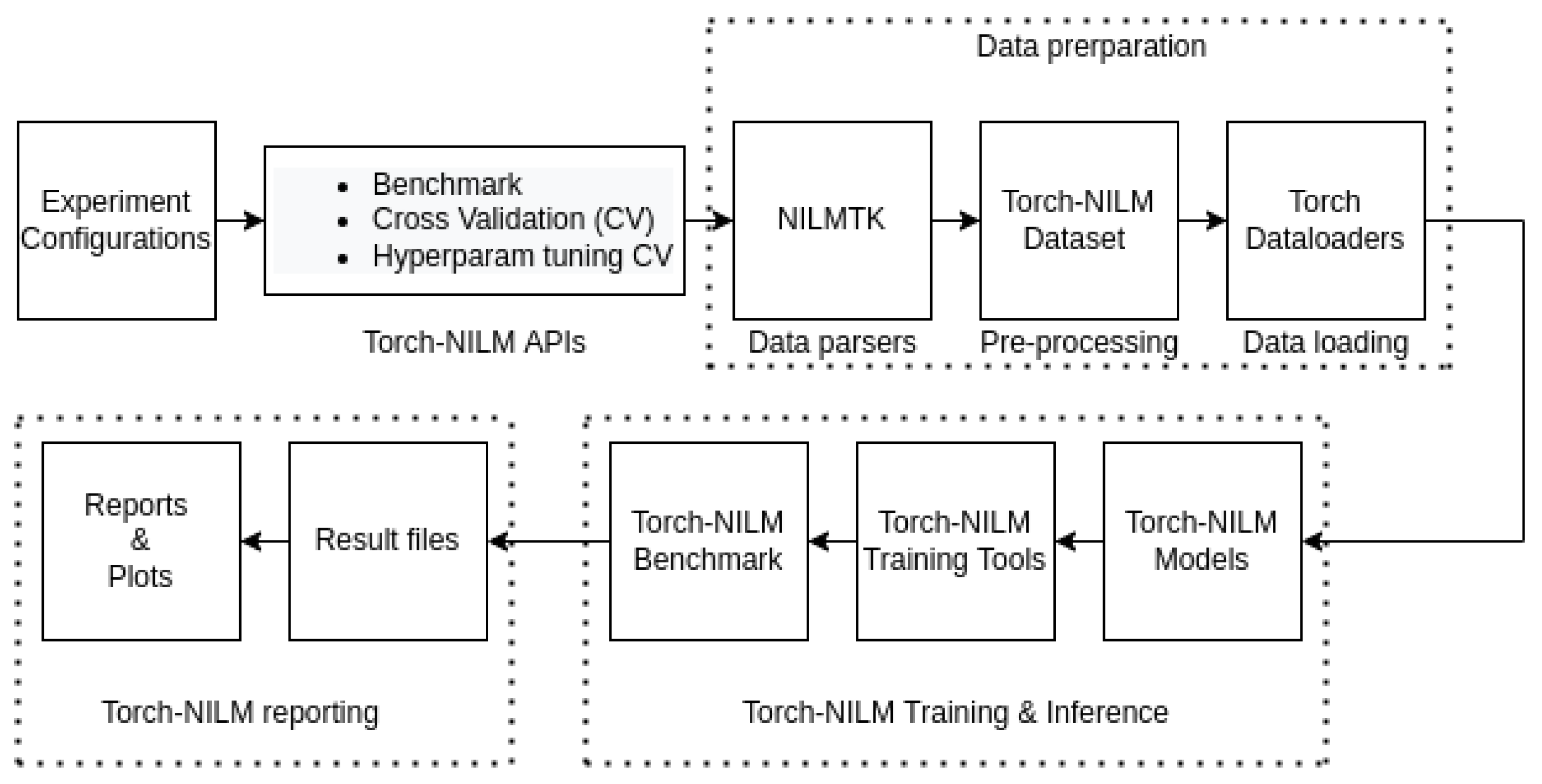
A simplified overview of the Torch-NILM experiment setup is depicted in Figure 1. The processes under the dashed lines are fully automated and easily modifiable. Hence, the user is only responsible for the experiment configuration and the API selection, whereas every component can be altered to fit different use-cases.
4. Torch-NILM APIs
Torch-NILM experiment APIs are callable methods of the NILMExperiments class, which is located in lab modules under nilm experiments. Currently, three basic APIs are provided: the benchmark, the cross-validation and the hyperparameter-tuning cross-validation. The function and usefulness of the provided APIs are discussed in the next subsections.
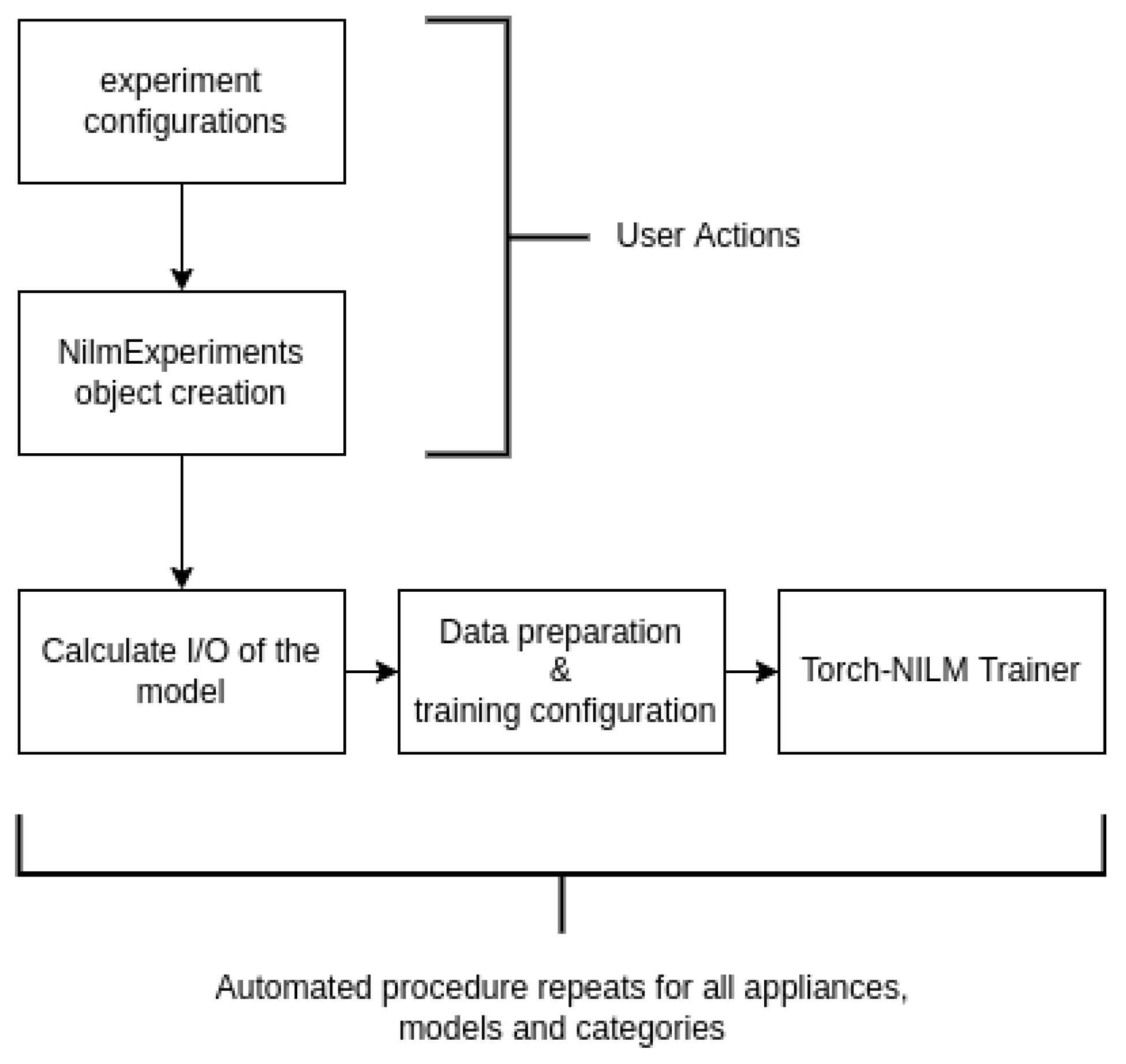
Every experiment API follows the basic set of steps presented in Figure 2. The user is responsible for only two things. For starters, to define the basic experiment configurations such as the target appliances, the number of epochs, the desired models and their hyperparameters, the project name, etc. These configurations are analysed in one of the following sections. Secondly, to create a NILMExperiments object to pass the configurations to. The rest of the procedure is controlled entirely of the NILMExperiments object and it consists of three main processes which repeat for every appliance, model and experiment category in an automated manner. At first, the input and the output of the model are calculated depending on the user-defined preprocessing schema. Then, the dataloaders and the training parameters are prepared. Finally, all the settings are passed to the Torch-NILM Trainer to conduct the training and inference.
4.1. Benchmark API
The Benchmark is essentially a four-part stress test with gradual difficulty. The model under evaluation goes through four different scenarios based on the methodology presented by Symeonidis et al. [13]. The first scenario contains experiments where training and inference are performed on data measurements collected from a single house. Inference and training time periods should not overlap. These experiments are considered easy for powerful models. The second benchmark category is composed of experiments where inference is applied on data measurements from different households in comparison to the training process. Obviously, the difficulty in this scenario is higher since different households demonstrate different energy activity and probably different appliances.
In both the remaining two benchmark scenarios, training is executed on data that are drawn from different buildings of the same dataset, but the evaluation differs for each scenario. In particular, in the third scenario, data are drawn from the same dataset as the dataset that was used during training. On the other hand, in the last category of experiment, a different dataset is used for inference.
In Torch-NILM, the benchmark is used under a specific nomenclature. This was because scenarios 1–2 and 3–4 share the same training process and only the inference data are different. Thus, the benchmark is executed faster. Scenarios 1–2 refer to training in one house and testing on a different house, which resulted in the name Single. Similarly, scenarios 3–4 are noted as Multi experiments. The name conventions between the original work of Symeonidis et al. [13] and Torch-NILM are summarised in Table 1.
4.2. Cross-Validation API
As the name suggests, cross-validation could be used in order to perform K-fold cross-validation on preselected dates. Cross-validation is mostly used in situations where the data are limited [33,34]. In NILM research, this is a very common scenario since many public data sets contain limited period of measurements and/or from single households. The pseudo-code of the developed cross-validation is presented in Algorithm 1. In cross-validation API implementation, the configuration is the same as the Benchmark API. The main difference is that due to the nature of K-fold cross-validation, training and inference are applied on the same data. The result is the average of the performance metrics for all the folds.
| Algorithm 1 cross-validation Implementation |
|
4.3. Hyperparameter Tuning Cross-Validation API
Hyperparameter tuning is an unavoidable step in machine learning during definition of the best parameters per situation. This can be performed with multiple repetitions of the benchmark, followed by results comparison. In order to save time, cross-validation can be used to search the hyperparameter space. Hence, we implemented the hyperparameter-tuning cross-validation experiment.
To conduct a hyperparameter search, multiple versions of the model should be defined. Then K-fold cross-validation for each version is executed. Finally, the user can decide which model is the best by comparing the results produced by the different model versions.
5. Data Preparation
A crucial step before the training of a neural network is data preparation, a set of methods that arrange the data into an appropriate format. The preparation consists of three main processes: the data parsing, the preprocessing and the data loading to the deep learning training. Based on the experiment, data preparation was conducted with the use of a different custom Dataset class. These classes were implemented to cover Single and Multi building experiment categories and can be found inside the datasources module.
5.1. Data Parsing
The parsing of the data is being handled by the NILMTK package. The data should be in a NILMTK-compatible format. This format was inspired by the REDD dataset arrangement [35]. In order to properly load a dataset, two classes were implemented and can be found in the datasources module; the DatasourceFactory; and the Datasource. Datasource objects contain methods that load the desired meter measurements. The DatasourceFactory is responsible for creating different Datasources objects that are based on various data sets.
5.2. Datasets and Appliances
Currently, Torch-NILM is compatible with all the public datasets that NILMTK can parse. In the current study, the following datasets are used: UK-DALE [36], REDD [35] and REFIT [37]. UK-DALE and REFIT are composed of measurements drawn from UK households, while REDD contains data from the USA. These datasets were chosen based on the following factors:
- The popularity among NILM researchers.
- The variety of appliances and households.
- The volume of the data. REFIT contains up to 20 households for more than a year of measurements and UK-DALE contains 5 households for 3 years of data.
- The granularity of the data, which is from 1 Hz up to 1/8 Hz.
Household electrical appliances are divided into three categories based on their operation cycle [3,38]: Single state, continuous and Multi-state operation appliances. Single-state appliances operate on a certain power level without any intermediate stages of operation. A common example is the resistive type of appliances, where a resistor is heated until it reaches a desired temperature and then it is turned off. Multi-state appliances have intermediate stages in their operation cycle. The power level of each stage may differ, resulting in a more complicated power-consumption signature. Appliances with continuous operation follow an all-day repeated consumption pattern with a varying power level.
For all the benchmark experiments, five electrical appliances were used: the washing machine, the dishwasher, the fridge, the kettle and the microwave. These appliances are found in the majority of NILM papers due to their different operation characteristics and their popularity among households. The active power level of operation for washing machines and dishwashers is within a range of 1200 to 2500 Watts. Hence, these devices are considered power intensive and accurate disaggregation is critical for a household energy-management system. The fridge operates at a very low power level; usually under 200 Watts. Although it is not a power-intensive appliance, it operates 24 h a day all year round. Its accumulated energy consumption is an important part of the total household consumption over a given period.
The kettle and the microwave are cooking micro-appliances. These type of appliances are very popular and they come in many variations among manufacturers. Usually, their operation cycle lasts for limited time periods during the day. The operation of the kettle is simple; it boils water very quickly. Hence, kettle end-uses produce low-duration pulses with relatively high active power from 1000 to 2000 W. On the other hand, the microwave has a more complicated operation with many different programs in various power levels and duration cycles. Thus, accurate disaggregation of these appliance could reveal the power of the model in detecting short appliance end-uses during a given time period.
5.3. Data Preprocessing
The data preprocessing contains the following steps which are summarised in Table 2. For starters, the time series are aligned in terms of time. Next, the missing values are filled. Currently two methods are supported for filling the missing values; zero replacement and linear interpolation. Then, normalisation of the data is applied. Data normalisation or data scaling is important because neural networks are easier to train when dealing with small values. This is due to the gradient descent optimisation algorithm [39]. Values on the same or a similar scale help the gradient descent algorithm to converge more quickly towards the minima. In Torch-NILM, two methods of data normalisation are provided: max division normalisation and standardisation. The user can choose between these two methods by defining the proper argument for Normalisation.
Standardisation is a normalisation technique where the values are centred around the zero mean with a unit standard deviation. Standardisation is given by (1):
where Z is the standardised value, x the observed value, the mean of the sample and the standard deviation.
Another common scaling method in NILM [18,20] is the division by the max value of the time series, resulting in simply normalised values by the max as shown in (2):
where is the normalised value, x the observed value and the max value of the sample.
After the scaling of the data, the arrangement of input and output is performed. Often, NILM is seen as a sequence-to-sequence type of problem [18,40], where the output has the same length of the input. Over the years, more methods were proposed and adapted by researchers. Some methods use sliding windows on the input in order to estimate only one point in the output [20,41]. Other methods consider different sizes of input and output as proposed by [42]. Torch-NILM supports the following four popular methods: sequence-to-sequence learning, proposed by [40]; sliding window, introduced by [20]; the sequence-to-point method proposed by [41] and sequence to subsequence [42].
On the other hand, sequence-to-point learning receives a window of mains measurements and outputs the appliance power consumption at the midpoint of the window: -> . A variation of this method is the sliding window approach, where the network estimates the appliance power consumption at the last point of the window. Sequence to subsequence is a mix between sequence-to-sequence and sequence-to-point methods, where the output is a smaller sequence of points than the input sequence, centred at the midpoint of the input window as shown in Figure 3. In order to select between these options, the Torch-NILM user should define the proper value for the Preprocessing Method.
As the final step of data preparation, Torch-NILM provides a method to add Gaussian noise on the input series. In situations of data shortage, adding noise can function as a regulariser for the neural network and can reduce overfitting. The percentage of the added noise can be controlled with a noise factor, a factor to multiply a Gaussian noise signal, which will be added to the normalised mains timeseries. The noise factor is within the range 0–1, with zero meaning no added noise. The noise follows Gaussian distribution (mu = 0, sigma = 1). The final input mains signal is given by (3):
After the data preprocessing is finalised, the data are ready to be provided to the NILM-Trainer for training and inference. For efficient data loading, Pytorch provides built-in Dataloader objects.
6. Training and Inference
Torch-NILM comes with six different neural network models developed in Pytorch. These models are proven to have different qualities, pros and cons. Hence, NILM researchers are given a powerful set of baseline models with which to compare their original network. Additionally, the architectural differences of these models may inspire the researchers to design and implement their own solution. A brief introduction for each model is presented below. For more information, please refer to the corresponding papers.
6.1. Torch-NILM Models
Denoising autoencoder architecture was originally proposed by Vincent et al. [43]. This model attempted to remove noise from an input and create a clean output. It was adapted in NILM by Kelly and Knottenbelt [18], where the mains power consumption was considered as the noisy signal and the appliance consumption as the target. In that work, DAE was used in a sequence-to-sequence learning framework. To adapt the architecture to accept more framing methods, a final linear layer was added. This layer adjusted the output to the desired shape. The architecture is presented in Figure 4:
Sequence-to-point (S2P)was proposed by Zhang et al. [19]. The model consisted of a series of convolutional layers with ReLU activations between them. Even though the model has millions of parameters, the training time was considerably small due to the fact that convolution operations were executed in parallel. Originally the output of the model was the appliance consumption at the midpoint of the input window. The architecture is shown in Figure 5.
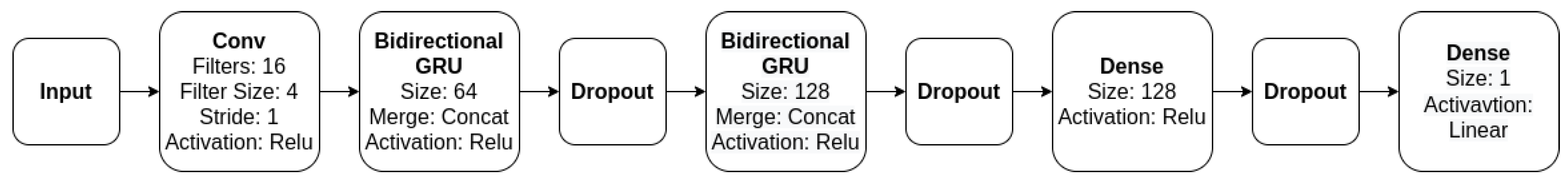
The main component of Window GRU (WGRU) is a pair of two bidirectional GRU layers. The GRU layer [44] is a type of recurrent neural network which is more computationally efficient than the LSTM. WGRU was proposed by Krystalakos et al. [20] and has four intermediate layers in total. Between the layers, dropout is used [45]. In the original paper, a sliding window approach was used to estimate the power consumption of the device at the end of the input window. The architecture is depicted in Figure 6.
Inspired by WGRU, Virtsionis-Gkalinikis et al. [24] proposed Self-Attentive Energy Disaggregator (SAED), architecture that combines GRU with an attention mechanism. The attention mechanism after the convolution layer helps the model to focus on the most important features of the input sequences. Compared to WGRU, SAED is many times faster and smaller in size. In the current work, the multi-head attention is also supported. This network was also proposed with the sliding-window learning schema. Figure 7 summarises the SAED architecture.
Langevin et al. [22] proposed a UNET [46] type of variational autoencoder (VAE) with skip connections to tackle the problem of NILM. VAE was originally proposed by Kingma and Welling [47] in an effort to conduct variational inference [48] on large-scale datasets in an efficient manner. Essentially, a VAE model aims to approximate the posterior distribution, which is intractable in most of the cases. The authors of VAE-NILM [46] claimed that the proposed architecture learns more complex power consumption signatures, resulting in better disaggregation and generalisation compared to other state-of-the-art deep learning solutions. In the original implementation, a sequence-to-sequence scheme is used, where the output is the same size as the input. The main component of VAE-NILM is IBN-Net block, which contains a series of convolution and batch normalisation layers. VAE-NILM is presented in Figure 8.
NFED is architecture proposed by Nalmpantis et al. [25] in 2022. This a rather deep neural network that was inspired by the FNET [49], a variant of the Transformer architectures [50,51,52,53] where the attention layer was replaced by Fourier transformation. Fourier transformation is used as a more efficient alternative to the attention mechanism. In the original paper, NFED was compared with WGRU and a S2P model performing on par with less learning parameters using the sliding window approach. NFED consists mainly of fully connected and normalised layers as shown in Figure 9, with some additional residual connections.
6.2. Torch-NILM Training Tools
One of the goals that drove the creation of Torch-NILM was the need to create many deep learning models easily. Often, the architecture and the training loop are implemented together in a large-scale code block. Even though using this design pattern may seem easy and fast, it has some drawbacks. To begin with, the code could become difficult to read and maintain. Furthermore, developing a new model necessitates re-implementing the training loop code again, which is inefficient. Finally, difficulties may arise when introducing alterations to the training loop or the model. As a result, this design pattern makes the creation of many architectures a non-trivial task.
In Torch-NILM the training loop is separated from the model architecture. Hence, the development and modification of models and the training process is easier and maintainable. In order to achieve the latter, Torch-NILM offers deep learning training tools. These tools are based on Pytorch Lightning, a framework to simplify Pytorch code into clean and easy-to-modify snippets.
The training tools are organised into different classes to match every training occasion. Each training tool class contains all the necessary steps to train, evaluate and save a model in Pytorch such as forward and backward pass, loss function and optimiser configuration, etc. In addition, all the available Pytorch Lightning callbacks can be used to modify the training loop during execution. Callbacks are blocks of reusable code which are called after finishing a training epoch and can be easily customised to fit many needs. Some of these callbacks are early stopping and model-checkpoint saving.
Currently, two types of training tools are provided: ClassicTrainingTools and VIBTrainingTools. Inside ClassicTrainingTools, the necessary steps for applying training inference on regression type problems are contained, where mean square error loss function (MSE) is used. MSE loss is calculated as shown in (4), where n is the number of data points, the i-th actual value and the prediction.
The set of VIBTrainingTools supports variational inference training, where the loss function is the evidence lower bound (ELBO) given by (6). Given an input , variational inference aims to learn posterior distribution rather than discrete values. This means that the model could approximate data points that have not been encountered during training. Resulting from the Bayes rule, as shown in (5), the posterior distribution is equal to the likelihood times the prior divided by the evidence . Due to the fact that the evidence is intractable, the true posterior can not be computed analytically in most cases. In order to estimate the true posterior, the ELBO loss function is used, where is the approximation of the true posterior. To measure the information lost when approximating the posterior, Kullback Leibler divergence (KL) is used [54].
All the supported models are trained using ClassicTrainingTools, except the VAE model where VIBTrainingTools are used. In order to use the training tools that match each model, the TrainingToolsFactory class was implemented. This class is the bridge between the model and the training tools. It should be noted that the Torch-NILM training tools also provide methods to compute the desired performance metrics after the inference is concluded. The metrics used are described in the following section.
6.3. Evaluation Metrics
In order to evaluate the performance of a NILM model, three metrics are used: score, mean absolute error (MAE) and relative error in total energy (RETE). score measures the ability of the model to detect the change of state (On/Off) of an appliance. As shown in (7), it is the harmonic mean of precision and recall given by the Equations (8) and (9), accordingly. MAE is used to quantify how much the estimated power consumption differs from the ground truth consumption. It is an absolute measure computed in Watts and calculated is given by (10), where T is the length of the predicted sequence, the estimated electrical power consumption and the true value of active power consumption at moment t. Likewise, RETE evaluates the model’s ability to predict the actual electric power consumption of an appliance. It is a dimensionless measure and is calculated by (11), where and E are the estimated and the true value of total energy correspondingly. All the aforementioned metrics are implemented in class NILMmetrics in the utils module.
6.4. Torch-NILM Benchmark
The benchmark module was created considering the reproducibility of the results. This module contains files with preselected dates for all the training and testing testing scenarios for the five appliances of interest: the washing machine, dishwasher, fridge, kettle and microwave. All the dates were selected in such a way that they contained enough appliance end-uses for producing disaggregation results.
Inside the module, three volumes of dates are provided to cover the potential needs of the researcher. For all scenarios, the large volume contains 8 and 4 months for training and testing, correspondingly. Similarly, the small volume contains 4 months for training and 2 months for testing, whereas the cv volume provides 10 months of training dates. Some of the selected houses for all the experiment categories are depicted in Table 3. In the provided code there are more selected households for each case, but we found those presented in Table 3 to contain enough appliance end-uses for proper disaggregation.
7. Torch-NILM Reporting
Torch-NILM provides a reporting module to easily conduct comparisons between models. This module is responsible for executing two tasks. Firstly, it creates the report files for every training and inference session of a model. The report files contain the performance evaluation files, the output of the model and the model weights file for each run. Secondly, it compiles all of the assessment reports and builds a final report file along with a set of comparison graphs between the models for fast visual inspection of the results. The reporting module is built mostly on core Python, Pandas [6] and Plotly [55] libraries.
In order to obtain more reliable results, a common approach is to execute each experiment multiple times. The final result is then computed as the average of all the different executions. The variance of the experiment results indicate how stable a model is; low variance means a stable model, high variance shows that the model produces very different predictions every time. In NILM applications, models with low variance are preferred. The reporting module supports the calculation of various statistical measures over the results of different runs of the same model. The statistical measure that are currently supported in the reporting module are presented in Table 4.
The final report is exported in xlsx format with multiple sheets. Each sheet contains the results for the electrical appliance of interest. In every sheet, each row contains the statistical measures of the performance metrics for every model. The exported comparison graphs are based on the final report results. Two type of graphs are currently supported: bar plots and radar/spider plots.
8. Experiment Configurations
In order to create an experiment object, there are some basic configurations to be set. To begin with, the user must provide the general experiment parameters. These parameters are:
- The maximum number of training epochs. Torch-NILM uses the early stopping callback, which stops the training if the loss does not decrease after a number of patience epochs.
- The number of iterations that every experiment will be executed.
- The sample period of the data. In case the sampling period is lower or higher than the original sampling of the data then sub-sampling or up-sampling is applied to match the desired sample period.
- The batch size that will be used for training and inference.
- The preprocessing method. Currently, four methods are supported: sequence-to-sequence learning, the sliding-window approach, the midpoint-window method and the sequence-to-subsequence approach.
- The inference cpu parameter controls whether the inference should be executed on CPU or GPU.
- The iterable dataset setting defines whether the training data should be loaded in memory gradually in batches or in one go.
- The train test split parameter defines the ratio of test and validation data.
- The cv folds setting is the number of folds in cross-validation experiments.
- The noise factor parameter controls the percentage of noise to add to the mains signal.
- The fixed window parameter is the length of the input sequence. If None is given then predefined windows are used for each model.
- The sub sequence setting is the length of the output sequence when sequence-to-subsequence preprocessing method is chosen.
- The list devices contains the target appliances.
- The experiment categories is the list of the desired benchmark categories (Single or Multi) to be executed.
After setting the general experiment parameters, the model hyperparameters for each API are required. The Benchmark and the CrossValidation APIs receive their settings in the same format, in a list called model hparams where all the desired architectures and their respective parameters are stored. On the other hand, the Hyperparameter tuning API receives a list that contains all the desired versions of the models of interest.
The final step is to define the project name, the experiment volume and which files should be exported. Specifically, if the parameter save timeseries is true then Torch-NILM saves the output of the models in a .csv format. Similarly, the parameters export plots and save model control whether comparison graphs and model weights will be saved.
All exported files, graphs and reports in Torch-NILM are saved in distinct project folders within the output folder. As a result, each project is structured in a logical manner, allowing the users to find the files they need easily. Figure 10 depicts an example of the file structure. There are three directories in each project, one for each API. The experiment results, exported graphs and saved models are all kept in distinct folders in each API directory. The results directory, which contains the final report, and the plots directory, which contains the performance comparison graphs, are the two key areas of interest for the user in this structure.
9. Torch-NILM in Use
This section presents the properties of Torch-NILM through a set of experiments. The structure is as follows. At first, a short performance verification is conducted in order to confirm the fact that Torch-NILM performs as expected. The verification was investigated through a performance comparison of the proposed solution with another already validated toolkit on the same input data. Then a benchmark case study was performed to highlight some important qualities of Torch-NILM.
9.1. Performance Verification
The reliability of the results is crucial for open source projects. Regarding Torch-NILM, the verification was performed with a results comparison between the suggested solution and a previously validated framework. The closest framework to Torch-NILM is the NILMTK-Contrib API [32], a software where state-of-the-art and baseline models are offered. In fact, some of the provided models are also included in Torch-NILM due to their popularity and effectiveness. As summarised in Table 5, the comparison results for one state-of-the-art model and three electrical appliances on the same data input confirm that Torch-NILM produces similar results to the verified software with 1.66% maximum percentage difference and 3.27% maximum percentage error. It should be noted that these toolkits are based on different deep learning frameworks, Pytorch and Tensorflow, and small differences are expected. All the experiments were executed on data from UK-DALE and the comparison was performed only on the MAE performance metric due to NILMTK-Contrib metrics shortage. Two weeks of data were used for training and one week for testing. Each experiment was executed five times with a different seed for five epochs. The same seeds were used between the two frameworks. All the experiments were performed on the same machine with a Titan Xp GPU.
9.2. Case Study
In order to demonstrate some of the qualities of the suggested toolkit, the benchmark was executed through the Benchmark API for three models as a case study: S2P, NFED and DAE, in both Single and Multi categories. The settings used for the experiments are presented below in Figure 11. All the scenarios were executed three times for 10 epochs, and batch size 1024 and inference was performed in GPU. The sliding-window schema was used and 10% of noise was added in the mains signal during training. Some of the produced results for the microwave are presented in Figure 12, Figure 13, Figure 14 and Figure 15. These graphs were generated automatically by Torch-NILM’s reporting module.
As shown in the results for the microwave, all models performed on par in terms of F1 in Single-type experiments, with S2P achieving better scores. Regarding MAE, the DAE showed the largest values, whereas NFED and S2P achieved similar performances. On the multi-type scenarios for the microwave, S2P showed the best performance with NFED being relatively close regarding the MAE error.
10. Conclusions
Despite the fact that deep learning is a popular approach for energy disaggregation, there are only a few NILM-oriented tools that properly assist the development and comparison of neural network topologies. As a result, without an organised pathway or a template, researchers must design their own set of tools, which often leads to non-reproducible results and difficult-to-read implementations. Additionally, the lack of a widely accepted benchmark poses further difficulties regarding the comparability of architectures. The proposed toolkit was created to address these issues. Torch-NILM offers APIs in order to easily develop experiments and comparisons with repeatable results. The combination of Pytorch’s strengths with an integrated benchmark process, a set of powerful baseline models and an effective set of training and reporting modules renders the proposed tool a robust solution to perform and develop NILM research.
Torch-NILM could be further developed/improved in the future in the following ways. Initially, implementing a modern looking graphical user interface would make the procedure of performing experiments much easier. In addition, further data-processing techniques and display graphs could be introduced. It would be also beneficial to add methods and models that support Multi-label classification techniques.
Author Contributions
Conceptualisation, N.V.G. and C.N.; methodology, N.V.G. and C.N.; software, N.V.G. and C.N.; validation, N.V.G., C.N. and D.V.; formal analysis, N.V.G. and C.N.; investigation, N.V.G. and C.N.; resources, D.V.; data curation, N.V.G. and C.N.; writing—original draft preparation, N.V.G.; writing—review and editing, N.V.G. and C.N.; visualisation, N.V.G.; supervision, D.V.; project administration, D.V.; funding acquisition, D.V. All authors have read and agreed to the published version of the manuscript.
Funding
This research has been co-financed by the European Regional Development Fund of the European Union and Greek national funds through the Operational Program Competitiveness, Entrepreneurship and Innovation, under the call RESEARCH–CREATE–INNOVATE (project code: T1EDK-00343(95699)-Energy Controlling Voice Enabled Intelligent Smart Home Ecosystem).
Institutional Review Board Statement
Not applicable.
Informed Consent Statement
Not applicable.
Data Availability Statement
Not applicable.
Acknowledgments
We gratefully acknowledge the support of the NVIDIA Corporation with the donation of the Titan Xp GPU used for this research.
Conflicts of Interest
The authors declare no conflict of interest.
References
- Armel, K.C.; Gupta, A.; Shrimali, G.; Albert, A. Is disaggregation the holy grail of energy efficiency? The case of electricity. Energy Policy 2013, 52, 213–234. [Google Scholar] [CrossRef] [Green Version]
- Mahapatra, B.; Nayyar, A. Home energy management system (HEMS): Concept, architecture, infrastructure, challenges and energy management schemes. Energy Syst. 2019, 1–27. [Google Scholar] [CrossRef]
- Hart, G.W. Nonintrusive appliance load monitoring. Proc. IEEE 1992, 80, 1870–1891. [Google Scholar] [CrossRef]
- Batra, N.; Kelly, J.; Parson, O.; Dutta, H.; Knottenbelt, W.; Rogers, A.; Singh, A.; Srivastava, M. NILMTK: An open source toolkit for non-intrusive load monitoring. In Proceedings of the 5th International Conference on Future energy Systems, Cambridge, UK, 11–13 June 2014; pp. 265–276. [Google Scholar]
- Van Rossum, G.; Drake, F.L. Python 3 Reference Manual; CreateSpace: Scotts Valley, CA, USA, 2009. [Google Scholar]
- McKinney, W. Data structures for statistical computing in python. In Proceedings of the 9th Python in Science Conference, Austin, TX, USA, 28 June–3 July 2010; Volume 445, pp. 51–56. [Google Scholar]
- Harris, C.R.; Millman, K.J.; van der Walt, S.J.; Gommers, R.; Virtanen, P.; Cournapeau, D.; Wieser, E.; Taylor, J.; Berg, S.; Smith, N.J.; et al. Array programming with NumPy. Nature 2020, 585, 357–362. [Google Scholar] [CrossRef] [PubMed]
- Pedregosa, F.; Varoquaux, G.; Gramfort, A.; Michel, V.; Thirion, B.; Grisel, O.; Blondel, M.; Prettenhofer, P.; Weiss, R.; Dubourg, V.; et al. Scikit-learn: Machine learning in Python. J. Mach. Learn. Res. 2011, 12, 2825–2830. [Google Scholar]
- Abadi, M.; Agarwal, A.; Barham, P.; Brevdo, E.; Chen, Z.; Citro, C.; Corrado, G.S.; Davis, A.; Dean, J.; Devin, M.; et al. TensorFlow: Large-Scale Machine Learning on Heterogeneous Systems. 2015. Available online: tensorflow.org (accessed on 7 November 2015).
- Chollet, F. Keras. 2015. Available online: https://github.com/keras-team/keras (accessed on 21 November 2015).
- Paszke, A.; Gross, S.; Massa, F.; Lerer, A.; Bradbury, J.; Chanan, G.; Killeen, T.; Lin, Z.; Gimelshein, N.; Antiga, L.; et al. PyTorch: An Imperative Style, High-Performance Deep Learning Library. In Advances in Neural Information Processing Systems; Curran Associates, Inc.: Red Hook, NY, USA, 2019; Volume 32, pp. 8024–8035. [Google Scholar]
- Falcon, W. PyTorch Lightning. GitHub. 2019, Volume 3. Available online: https://github.com/PyTorchLightning/pytorch-lightning (accessed on 16 December 2019).
- Symeonidis, N.; Nalmpantis, C.; Vrakas, D. A Benchmark Framework to Evaluate Energy Disaggregation Solutions. In Proceedings of the International Conference on Engineering Applications of Neural Networks, Crete, Greece, 24–26 May 2019; pp. 19–30. [Google Scholar]
- Pal, M.; Roy, R.; Basu, J.; Bepari, M.S. Blind source separation: A review and analysis. In Proceedings of the 2013 International Conference Oriental COCOSDA Held Jointly with 2013 Conference on Asian Spoken Language Research and Evaluation (O-COCOSDA/CASLRE), Gurgaon, India, 25–27 November 2013; pp. 1–5. [Google Scholar] [CrossRef]
- Khan, N.; Haq, I.U.; Ullah, F.U.M.; Khan, S.U.; Lee, M.Y. CL-Net: ConvLSTM-Based Hybrid Architecture for Batteries; State of Health and Power Consumption Forecasting. Mathematics 2021, 9, 3326. [Google Scholar] [CrossRef]
- Haq, I.U.; Ullah, A.; Khan, S.U.; Khan, N.; Lee, M.Y.; Rho, S.; Baik, S.W. Sequential Learning-Based Energy Consumption Prediction Model for Residential and Commercial Sectors. Mathematics 2021, 9, 605. [Google Scholar] [CrossRef]
- Ullah, F.U.M.; Khan, N.; Hussain, T.; Lee, M.Y.; Baik, S.W. Diving Deep into Short-Term Electricity Load Forecasting: Comparative Analysis and a Novel Framework. Mathematics 2021, 9, 611. [Google Scholar] [CrossRef]
- Kelly, J.; Knottenbelt, W. Neural nilm: Deep neural networks applied to energy disaggregation. In Proceedings of the 2nd ACM International Conference on Embedded Systems for Energy-Efficient Built Environments, Seoul, Korea, 4–5 November 2015; pp. 55–64. [Google Scholar]
- Zhang, C.; Zhong, M.; Wang, Z.; Goddard, N.; Sutton, C. Sequence-to-point learning with neural networks for nonintrusive load monitoring. In Proceedings of the Thirty-Second AAAI Conference on Artificial Intelligence, New Orleans, LA, USA, 2–7 February 2018. [Google Scholar]
- Krystalakos, O.; Nalmpantis, C.; Vrakas, D. Sliding window approach for online energy disaggregation using artificial neural networks. In Proceedings of the 10th Hellenic Conference on Artificial Intelligence, Thessaloniki, Greece, 18–20 May 2018; pp. 1–6. [Google Scholar]
- Yue, Z.; Witzig, C.R.; Jorde, D.; Jacobsen, H.A. BERT4NILM: A Bidirectional Transformer Model for Non-Intrusive Load Monitoring. In Proceedings of the 5th International Workshop on Non-Intrusive Load Monitoring, NILM’20, Virtual Event, 18 November 2020; Association for Computing Machinery: New York, NY, USA, 2020; pp. 89–93. [Google Scholar] [CrossRef]
- Langevin, A.; Carbonneau, M.A.; Cheriet, M.; Gagnon, G. Energy disaggregation using variational autoencoders. Energy Build. 2022, 254, 111623. [Google Scholar] [CrossRef]
- Iqbal, H.K.; Malik, F.H.; Muhammad, A.; Qureshi, M.A.; Abbasi, M.N.; Chishti, A.R. A critical review of state-of-the-art non-intrusive load monitoring datasets. Electr. Power Syst. Res. 2021, 192, 106921. [Google Scholar] [CrossRef]
- Virtsionis-Gkalinikis, N.; Nalmpantis, C.; Vrakas, D. SAED: Self-attentive energy disaggregation. Mach. Learn. 2021, 1–20. [Google Scholar] [CrossRef]
- Nalmpantis, C.; Virtsionis Gkalinikis, N.; Vrakas, D. Neural Fourier Energy Disaggregation. Sensors 2022, 22, 473. [Google Scholar] [CrossRef] [PubMed]
- Kukunuri, R.; Aglawe, A.; Chauhan, J.; Bhagtani, K.; Patil, R.; Walia, S.; Batra, N. EdgeNILM: Towards NILM on Edge Devices. In Proceedings of the 7th ACM International Conference on Systems for Energy-Efficient Buildings, BuildSys’20, Virtual Event, 18–20 November 2020; Association for Computing Machinery: New York, NY, USA, 2020; pp. 90–99. [Google Scholar] [CrossRef]
- Athanasiadis, C.; Doukas, D.; Papadopoulos, T.; Chrysopoulos, A. A Scalable Real-Time Non-Intrusive Load Monitoring System for the Estimation of Household Appliance Power Consumption. Energies 2021, 14, 767. [Google Scholar] [CrossRef]
- Athanasiadis, C.L.; Doukas, D.I.; Papadopoulos, T.A.; Barzegkar-Ntovom, G.A. Real-Time Non-Intrusive Load Monitoring: A Machine-Learning Approach for Home Appliance Identification. In Proceedings of the 2021 IEEE Madrid PowerTech, Madrid, Spain, 28 June–2 July 2021; pp. 1–6. [Google Scholar]
- Tabatabaei, S.M.; Dick, S.; Xu, W. Toward non-intrusive load monitoring via multi-label classification. IEEE Trans. Smart Grid 2016, 8, 26–40. [Google Scholar] [CrossRef]
- Nalmpantis, C.; Vrakas, D. On time series representations for multi-label NILM. Neural Comput. Appl. 2020, 32, 17275–17290. [Google Scholar] [CrossRef]
- Athanasiadis, C.L.; Papadopoulos, T.A.; Doukas, D.I. Real-time non-intrusive load monitoring: A light-weight and scalable approach. Energy Build. 2021, 253, 111523. [Google Scholar] [CrossRef]
- Kukunuri, R.; Batra, N.; Pandey, A.; Malakar, R.; Kumar, R.; Krystalakos, O.; Zhong, M. NILMTK-Contrib: Towards reproducible state-of-the-art energy disaggregation. In Proceedings of the AI for Social Good Workshop, Virtual Event, 7–8 January 2021. [Google Scholar]
- Ng, A.Y. Preventing “Overfitting” of Cross-Validation Data. In Proceedings of the Fourteenth International Conference on Machine Learning, ICML’97, Nashville, TN, USA, 8–12 July 1997; Morgan Kaufmann Publishers Inc.: San Francisco, CA, USA, 1997; pp. 245–253. [Google Scholar]
- Deisenroth, M.P.; Faisal, A.A.; Ong, C.S. Mathematics for Machine Learning; Cambridge University Press: Cambridge, UK, 2020. [Google Scholar]
- Kolter, J.Z.; Johnson, M.J. REDD: A public data set for energy disaggregation research. In Proceedings of the Workshop on Data Mining Applications in Sustainability (SIGKDD), San Diego, CA, USA, 21 August 2011; Volume 25, pp. 59–62. [Google Scholar]
- Jack, K.; William, K. The UK-DALE dataset domestic appliance-level electricity demand and whole-house demand from five UK homes. Sci. Data 2015, 2, 150007. [Google Scholar]
- Firth, S.; Kane, T.; Dimitriou, V.; Hassan, T.; Fouchal, F.; Coleman, M.; Webb, L. REFIT Smart Home Dataset. Available online: https://repository.lboro.ac.uk/articles/dataset/REFIT_Smart_Home_dataset/2070091/1 (accessed on 16 June 2016).
- Dong, M.; Meira, P.C.M.; Xu, W.; Freitas, W. An Event Window Based Load Monitoring Technique for Smart Meters. IEEE Trans. Smart Grid 2012, 3, 787–796. [Google Scholar] [CrossRef]
- Montavon, G.; Orr, G.; Mller, K.R. Neural Networks: Tricks of the Trade, 2nd ed.; Springer: Berlin/Heidelberg, Germany, 2012. [Google Scholar]
- Sutskever, I.; Vinyals, O.; Le, Q.V. Sequence to Sequence Learning with Neural Networks. In Proceedings of the 27th International Conference on Neural Information Processing Systems, NIPS’14, Bangkok, Thailand, 18–22 November 2020; MIT Press: Cambridge, MA, USA, 2014; Volume 2, pp. 3104–3112. [Google Scholar]
- D’Incecco, M.; Squartini, S.; Zhong, M. Transfer Learning for Non-Intrusive Load Monitoring. IEEE Trans. Smart Grid 2020, 11, 1419–1429. [Google Scholar] [CrossRef] [Green Version]
- Pan, Y.; Liu, K.; Shen, Z.; Cai, X.; Jia, Z. Sequence-To-Subsequence Learning With Conditional Gan For Power Disaggregation. In Proceedings of the ICASSP 2020—2020 IEEE International Conference on Acoustics, Speech and Signal Processing (ICASSP), Barcelona, Spain, 4–8 May 2020; pp. 3202–3206. [Google Scholar] [CrossRef]
- Vincent, P.; Larochelle, H.; Bengio, Y.; Manzagol, P.A. Extracting and Composing Robust Features with Denoising Autoencoders. In Proceedings of the 25th International Conference on Machine Learning (ICML’08), Helsinki, Finland, 5–9 July 2008; pp. 1096–1103. [Google Scholar] [CrossRef] [Green Version]
- Chung, J.; Gulcehre, C.; Cho, K.; Bengio, Y. Empirical evaluation of gated recurrent neural networks on sequence modeling. In Proceedings of the NIPS 2014 Workshop on Deep Learning, Montreal, QC, Canada, 12 December 2014. [Google Scholar]
- Srivastava, N.; Hinton, G.; Krizhevsky, A.; Sutskever, I.; Salakhutdinov, R. Dropout: A simple way to prevent neural networks from overfitting. J. Mach. Learn. Res. 2014, 15, 1929–1958. [Google Scholar]
- Ronneberger, O.; Fischer, P.; Brox, T. U-Net: Convolutional Networks for Biomedical Image Segmentation. In Proceedings of the Medical Image Computing and Computer-Assisted Intervention—MICCAI 2015, Munich, Germany, 5–9 October 2015. [Google Scholar]
- Kingma, D.P.; Welling, M. Auto-Encoding Variational Bayes. arXiv 2014, arXiv:1312.6114. [Google Scholar]
- Blei, D.M.; Kucukelbir, A.; McAuliffe, J.D. Variational Inference: A Review for Statisticians. J. Am. Stat. Assoc. 2017, 112, 859–877. [Google Scholar] [CrossRef] [Green Version]
- Lee-Thorp, J.; Ainslie, J.; Eckstein, I.; Ontanon, S. FNet: Mixing Tokens with Fourier Transforms. arXiv 2021, arXiv:2105.03824. [Google Scholar]
- Choromanski, K.M.; Likhosherstov, V.; Dohan, D.; Song, X.; Gane, A.; Sarlos, T.; Hawkins, P.; Davis, J.Q.; Mohiuddin, A.; Kaiser, L.; et al. Rethinking Attention with Performers. In Proceedings of the International Conference on Learning Representations, Addis Ababa, Ethiopia, 26–30 April 2020. [Google Scholar]
- Katharopoulos, A.; Vyas, A.; Pappas, N.; Fleuret, F. Transformers are RNNs: Fast Autoregressive Transformers with Linear Attention. In Proceedings of the International Conference on Machine Learning (ICML), Virtual Event, 13–18 July 2020. [Google Scholar]
- Shen, Z.; Zhang, M.; Zhao, H.; Yi, S.; Li, H. Efficient Attention: Attention with Linear Complexities. arXiv 2018, arXiv:1812.01243. [Google Scholar]
- Kitaev, N.; Kaiser, L.; Levskaya, A. Reformer: The Efficient Transformer. In Proceedings of the International Conference on Learning Representations, Addis Ababa, Ethiopia, 26–30 April 2020. [Google Scholar]
- Joyce, J.M. Kullback-Leibler Divergence. In International Encyclopedia of Statistical Science; Springer: Berlin/Heidelberg, Germany, 2011; ISBN 978-3-642-04898-2. [Google Scholar] [CrossRef]
- Sievert, C. Interactive Web-Based Data Visualization with R, Plotly, and Shiny. Available online: https://plotly-r.com (accessed on 19 December 2019).
Figure 1.
A rough overview of the data flow in Torch-NILM. The dashed lines denote the fully automated process.
Figure 1.
A rough overview of the data flow in Torch-NILM. The dashed lines denote the fully automated process.

Figure 2.
The basic steps of an experiment API execution.

Figure 3.
An example of sequence-to-subsequence preprocessing method.

Figure 4.
Architecture of DAE.

Figure 5.
Architecture of S2P.

Figure 6.
Architecture of WGRU.

Figure 7.
Architecture of SAED.

Figure 8.
The VAE network. (a) UNET VAE architecture; (b) the IBN-NET block.

Figure 9.
The NFED neural network. (a) Fourier block; (b) NFED architecture.

Figure 10.
Torch-NILM results structure.

Figure 11.
Experiment parameters for case study using the Benchmark API: (a) Generic experiment parameters; (b) model hyperparameters.
Figure 11.
Experiment parameters for case study using the Benchmark API: (a) Generic experiment parameters; (b) model hyperparameters.

Figure 12.
Average model performance for Single categories of experiments.

Figure 13.
Average model performance for Single categories of experiments.

Figure 14.
Benchmark results for Microwave: (a) F1 comparison for Single category; (b) MAE comparison for Single category.
Figure 14.
Benchmark results for Microwave: (a) F1 comparison for Single category; (b) MAE comparison for Single category.

Figure 15.
Benchmark results for Microwave: (a) F1 comparison for Multi category of experiments; (b) MAE comparison for Multi category of experiments.
Figure 15.
Benchmark results for Microwave: (a) F1 comparison for Multi category of experiments; (b) MAE comparison for Multi category of experiments.


Table 1.
The benchmark name conventions used in Torch-NILM.
| Category 1 | Category 2 | Category 3 | Category 4 | |
|---|---|---|---|---|
| Torch-NILM | Single | Single | Multi | Multi |
| Benchmark [13] | Single-building NILM | Single-building learning and generalisation on the same dataset | Multi-building learning and generalisation on the same dataset | Multi-building learning and generalisation on a different dataset |
Table 2.
An overview of data preprocessing steps in Torch-NILM.
| Process | Description |
|---|---|
| Time series alignment | The mains and meter consumption time series are aligned in time axis. |
| Fill missing values | All the missing values in both mains and meter time series are either filled with zeros or with values calculated by linear interpolation. |
| Data scaling | The scaling or normalisation of the data is used to bring the data values in the same scale. The data scaling method is selected using the variable Normalisation. |
| Input/output schema | The alignment of the input/output is controlled by the variable Preprocessing Method. |
| Gaussian noise addition | Adding noise to the signal can function as a regulariser to tackle overfitting. The percentage of the added noise is controlled by the noise factor. |
Table 3.
Selected households for training and inference. For categories 1–3, UK-DALE houses were used for training and testing. For the Category 4 experiments, UK-DALE was used only in training. REFIT was used to evaluate the performance of the models in the disaggregation of the dishwasher and the kettle, whereas REDD was used for inference of the rest of the appliances.
| Single | Multi | |||||||
|---|---|---|---|---|---|---|---|---|
| Electrical Appliance | Category 1 | Category 2 | Category 3 | Category 4 | ||||
| Train | Test | Train | Test | Train | Test | Train | Test | |
| Washing Machine | 1 | 1 | 1 | 4 | 1, 5 | 2 | 1, 5 | 3 |
| Dishwasher | 1 | 1 | 1 | 2 | 1, 2 | 5 | 1, 2 | 2 |
| Fridge | 1 | 1 | 1 | 2 | 1, 2, 4 | 5 | 1, 2, 4 | 3 |
| Kettle | 1 | 1 | 1 | 5 | 1, 2, 4 | 5 | 1, 2, 4 | 2 |
| Microwave | 1 | 1 | 1 | 2 | 1, 2 | 5 | 1, 2 | 1 |
Table 4.
The supported statistical measures in Torch-NILM.
| Measure | Description |
|---|---|
| mean | The average of all the values of the desired performance metric across different runs. |
| median | The middle value of the desired performance metric across different runs. |
| minimum | The minimum of all the values of the desired performance metric across different runs. |
| maximum | The maximum of all the values of the desired performance metric across different runs. |
| 25th quartile | 25% of the observations are lower than this value. |
| 75th quartile | 75% of the observations are lower than this value. |
Table 5.
Torch-NILM versus NILMTK-Contrib: Performance verification. For the experiments, S2P architecture was used. The training for all experiments was performed with 15 days of data and the testing with 7 days of data. For all the scenarios, training and testing were applied on house 1 of UK-DALE.
| Appliance | Model | Torch NILM MAE [W] | NILMTK Contrib MAE [W] | Mean Absolute Difference [W] | Mean Percentage Difference [%] | Mean Percentage Error [%] |
|---|---|---|---|---|---|---|
| Washing M. | S2P | 0.56 | 1.66 | 3.27 | ||
| Dishwasher | S2P | 0.46 | 1.29 | 2.56 | ||
| Microwave | S2P | 0.22 | 1.61 | 3.17 |
Publisher’s Note: MDPI stays neutral with regard to jurisdictional claims in published maps and institutional affiliations. |
© 2022 by the authors. Licensee MDPI, Basel, Switzerland. This article is an open access article distributed under the terms and conditions of the Creative Commons Attribution (CC BY) license (https://creativecommons.org/licenses/by/4.0/).
Share and Cite
MDPI and ACS Style
Virtsionis Gkalinikis, N.; Nalmpantis, C.; Vrakas, D. Torch-NILM: An Effective Deep Learning Toolkit for Non-Intrusive Load Monitoring in Pytorch. Energies 2022, 15, 2647. https://doi.org/10.3390/en15072647
AMA Style
Virtsionis Gkalinikis N, Nalmpantis C, Vrakas D. Torch-NILM: An Effective Deep Learning Toolkit for Non-Intrusive Load Monitoring in Pytorch. Energies. 2022; 15(7):2647. https://doi.org/10.3390/en15072647
Chicago/Turabian StyleVirtsionis Gkalinikis, Nikolaos, Christoforos Nalmpantis, and Dimitris Vrakas. 2022. "Torch-NILM: An Effective Deep Learning Toolkit for Non-Intrusive Load Monitoring in Pytorch" Energies 15, no. 7: 2647. https://doi.org/10.3390/en15072647
Note that from the first issue of 2016, this journal uses article numbers instead of page numbers. See further details here.