
Optimal Management for EV Charging Stations: A Win–Win Strategy for Different Stakeholders Using Constrained Deep Q-Learning

 and
and
Abstract
:1. Introduction
- In contrast to prior strategies [19,20,21,22], the proposed strategy is a win–win for both stakeholders, i.e., the EV owners and the EV charging station operators. Fulfilling charging demands under agreed conditions is prioritized, and profit maximization from the charging station operator’s perspective follows.
- Although direct bench-marking against pre-published literature is difficult because of the different operating conditions and data used, the financial benefit that is achieved for the charging station herein is considerable and comparable to the profit achieved in the literature [22].
- A new training scheme is proposed for the Q-learning algorithm. The constraints imposed guarantee customer satisfaction, which is removed from the optimization objective to allow the RL agent to maximize EV charging station profit.
- The proposed strategy is easy to adjust, and a different balance/prioritization between stakeholders needs can be selected (see Equation (13)).
2. System Model
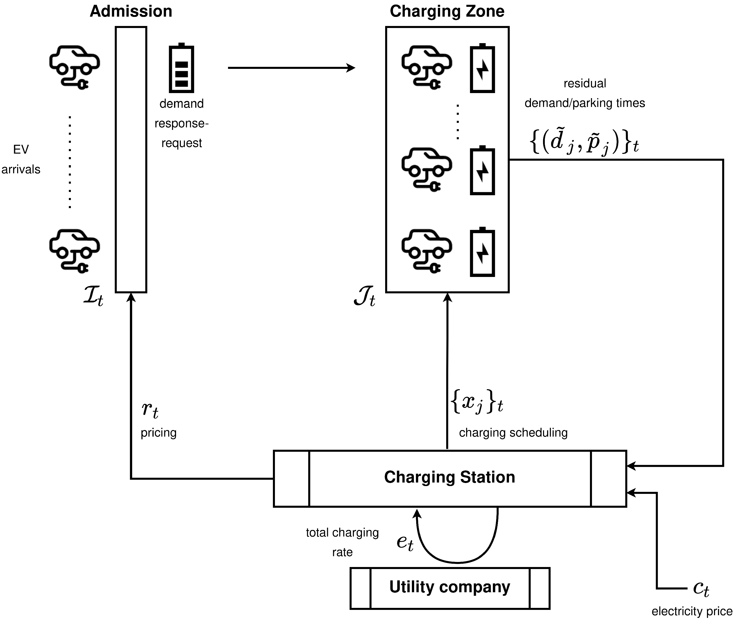
2.1. EV Charging Station Environment
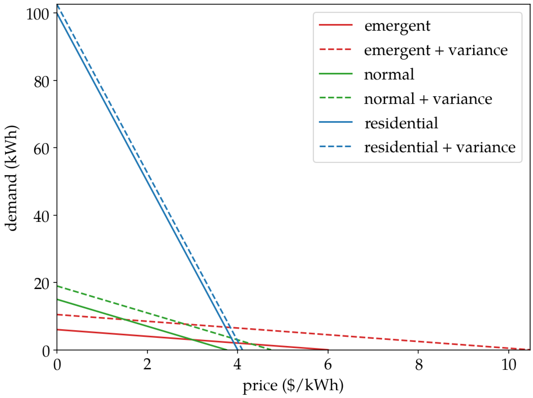
- EVs are price-sensitive; i.e., they adjust their charging demands based on the value of provided by the station. Thus, , where : is the demand–response function of EV i. Obviously, if EV i decides not to accept the presented rate, then . Additionally, note that the demand–response function is EV-specific in the general case.
- The price rate presented to will be constant for each EV in during its parking time.
- There is a fixed and finite number of individual chargers at the station, N. Thus, for all time slots t, , which means that at any given time, at most N EVs are parked at the station. Suppose the number of EVs, , that arrive at the station overflow the available chargers. In that case, a subset of is selected, in a first-come-first-served manner, to meet the parking capacity of the station.
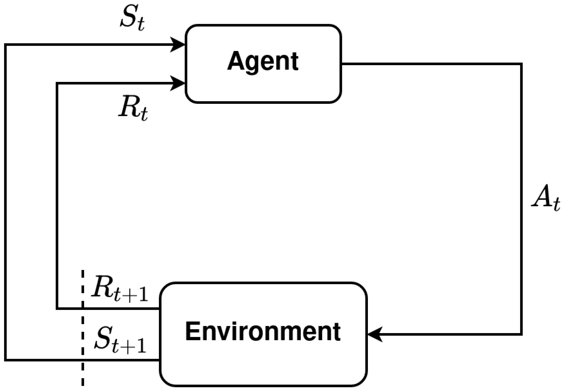
2.2. Problem Formulation Using the MDP Framework
- State/Observation Space
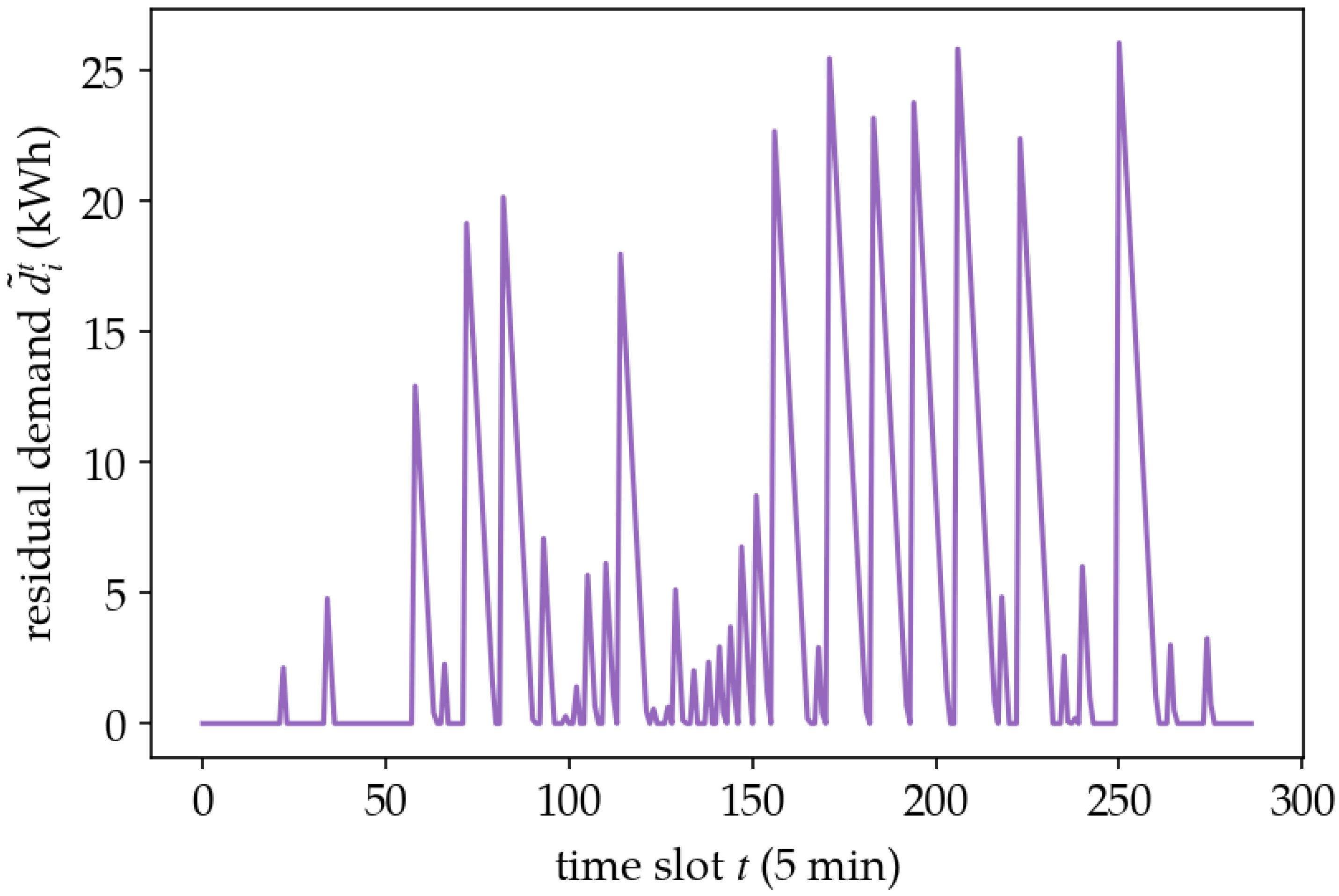
- The EVs that are parked at the station , along with the residual charging demand and parking time for each EV
- The newly arrived EVs,
- The last 24 h of values of the electricity price time series. Under the assumption that electricity price changes every slots, the 24 h historical values can be represented by:where . Equivalently, the number of samples M is given by:
- Action Space
- Reward Modeling
3. Proposed Solution
3.1. Constrained Least Laxity First
| Algorithm 1: Constrained least laxity first. |
| Require: Total charging rate Require: Total number of chargers N Require: Residual demand , Require: Residual parking time , Initialize remaining total charging rate for i = 1, N do Initialize Calculate laxity Initialize end for while do Find EV with the least laxity that has Update charging rate of EV : Calculate laxity of EV for next time slot : Update remaining total charging rate end while for i = 1, N do if then Constrain charging rate of EV i: end if end for Calculate constrained total charging rate |
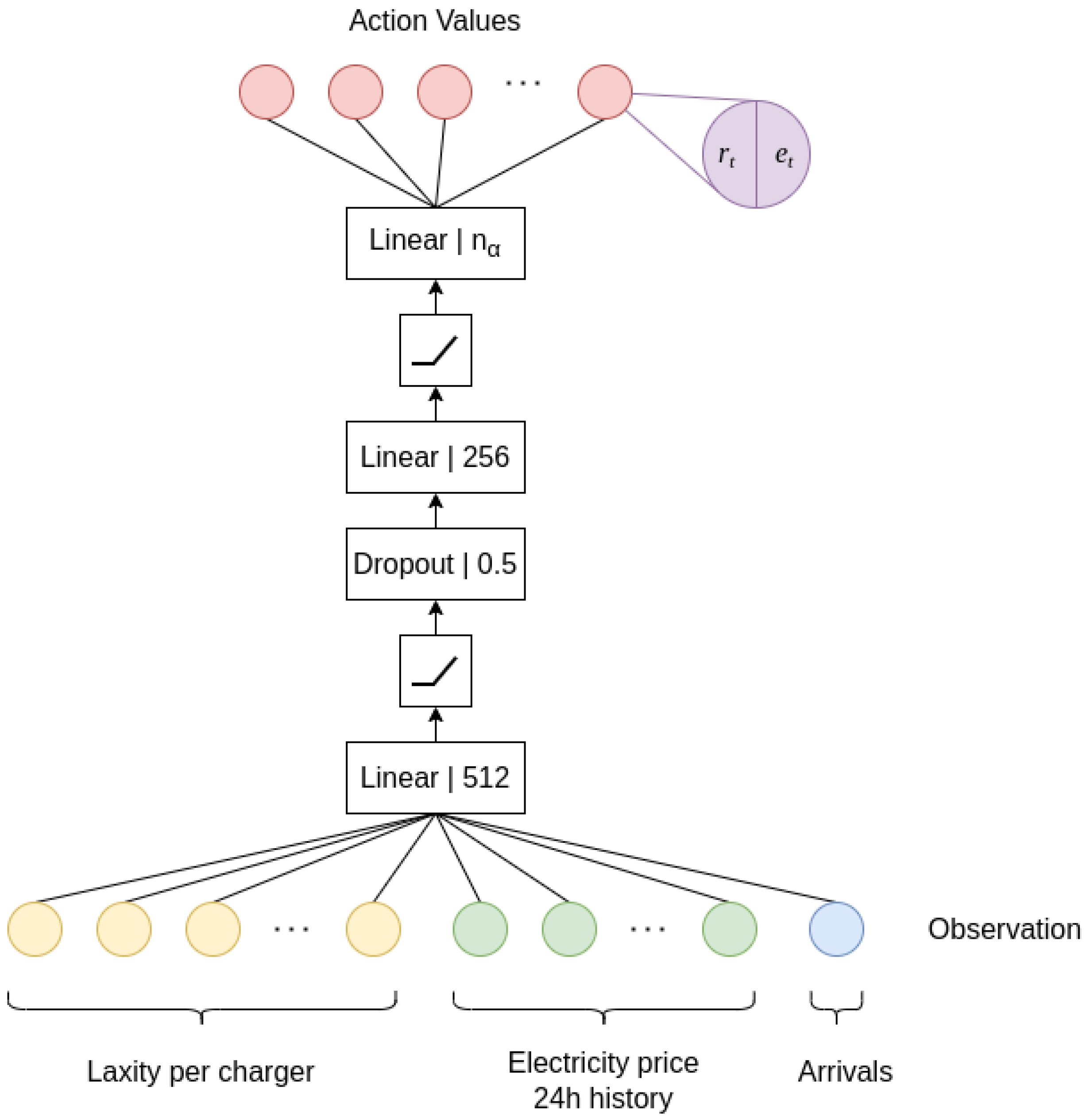
3.2. Agent Architecture
- N input nodes, each of which is the laxity of an EV at charger i, .
- One node corresponding to the number of EV arrivals observed at the admission zone of the station.
- Let be the L discrete price rate levels.
- Let be the K discrete charging rate levels.
- Then, the action space is:i.e., the Cartesian product of the discrete level sets, with cardinality
3.3. Training Approach
| Algorithm 2: Constrained deep Q-learning. |
| Require: Episode length schema function, h Require: Exploration rate schema, l Initialize replay memory D to capacity N Initialize action-value parametrized with random weights Initialize target action-value with weights for episode = 1, E do Initialize state Get current episode duration for t = 1, T do Get exploration rate With probability select a random action , otherwise select Constrain using the Constrained LLF algorithm Execute and observe reward and next state Store transition Sample random minibatch of transitions Set target
Perform a gradient descent step on Every C steps copy policy network weights to target network weights end for end for |
4. Evaluation Methodology
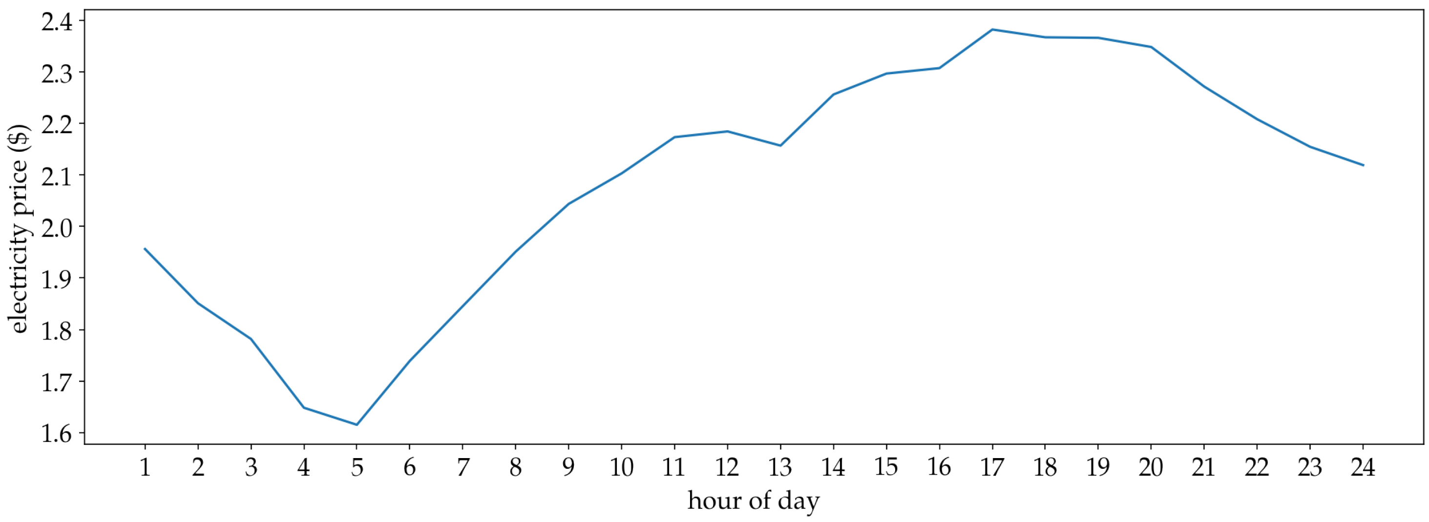
4.1. Datasets
- They were upsampled to 60 min intervals.
- They were scaled by a factor of and rounded to the closest integer.
- They were undersampled to 1 min intervals, by randomly distributing the 1 h samples to intermediate minutes using a uniform distribution.
4.2. Experimental Setup
- Chargers of the station: .
- Maximum charging rate per charger: According to the U.S. Department of Energy (https://afdc.energy.gov/fuels/electricity_infrastructure.html, accessed on 15 February 2022), most EVs on the road today are not capable of charging at rates higher than 50 kW. Thus, a more conservative approach of 30 kW was selected. Note that 22 kW is the closest standard charging rate (i.e., Level 2 EV charging), but the purpose of this work is to present a more general approach. kW
- Maximum total charging rate: kW.
- Time slot length: min.
- Episode duration: 1 day or 1440 min or 288 time slots.
- Discrete price rate levels: $.
- Discrete charging rate levels: kW.
- Cardinality of action space: .
- Demand–Response Function
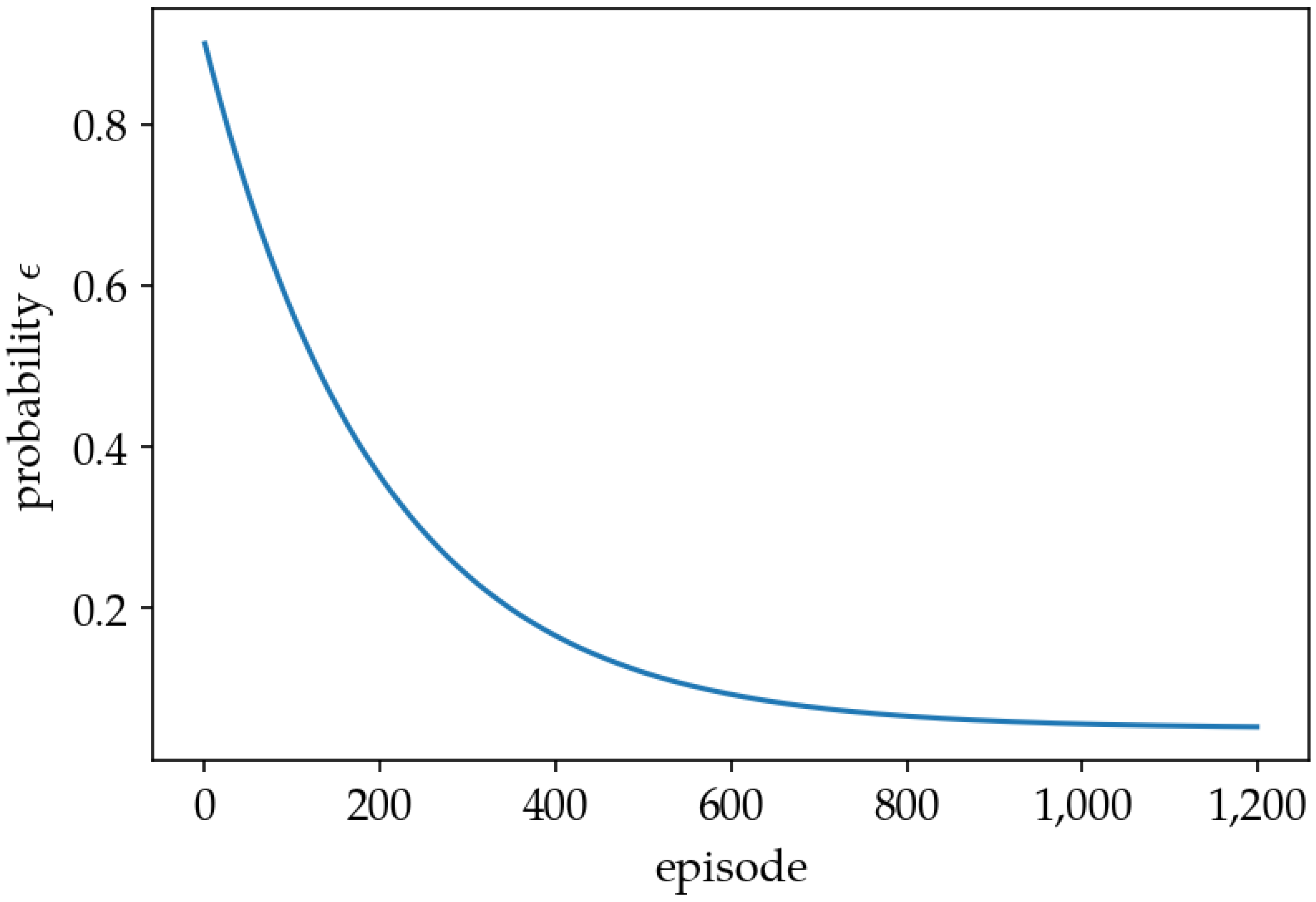
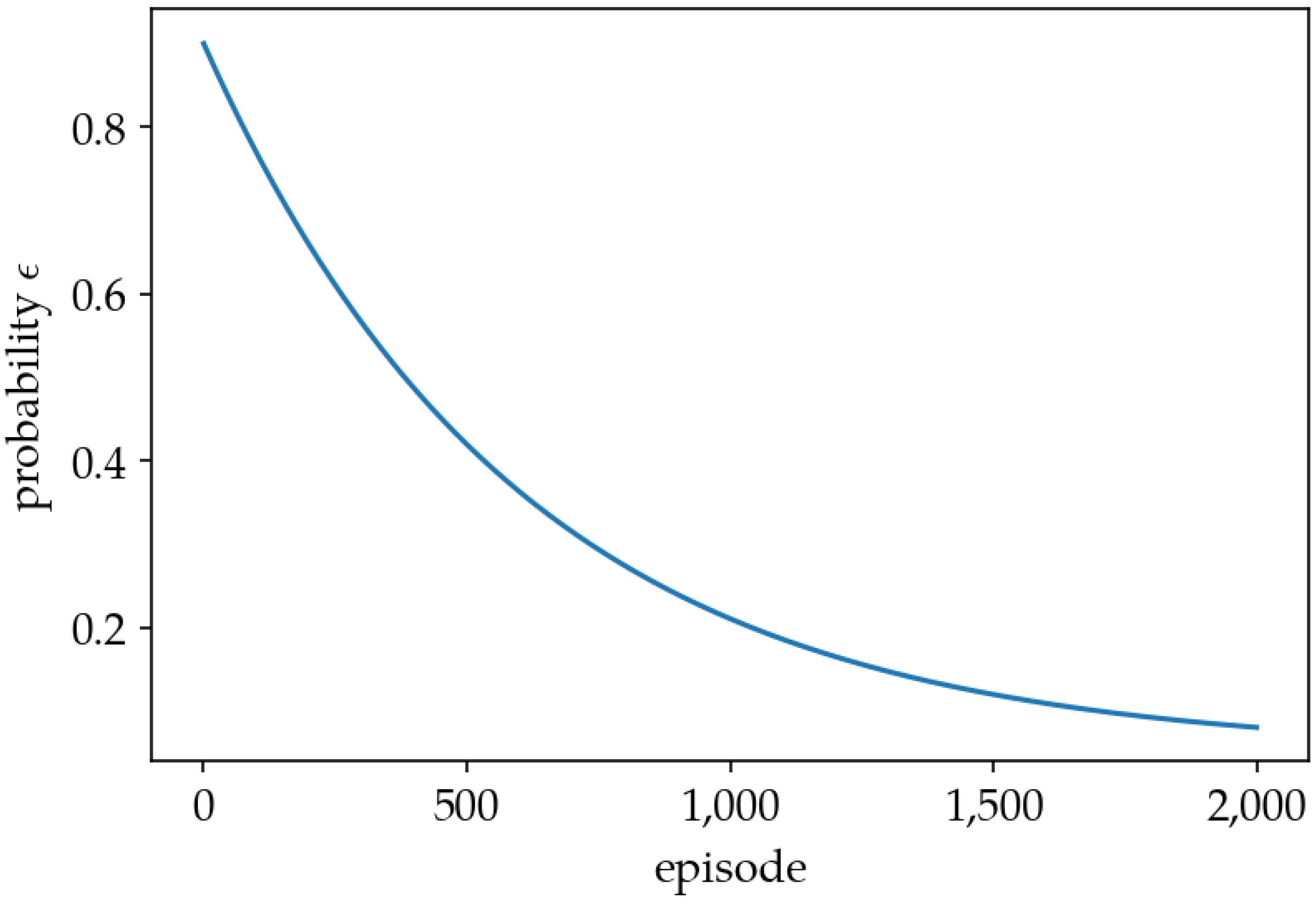
- -Greedy Policy
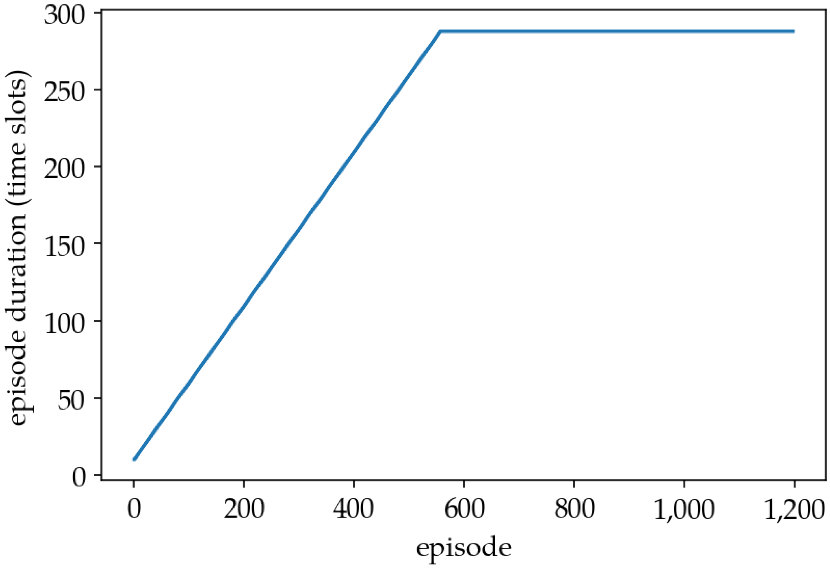
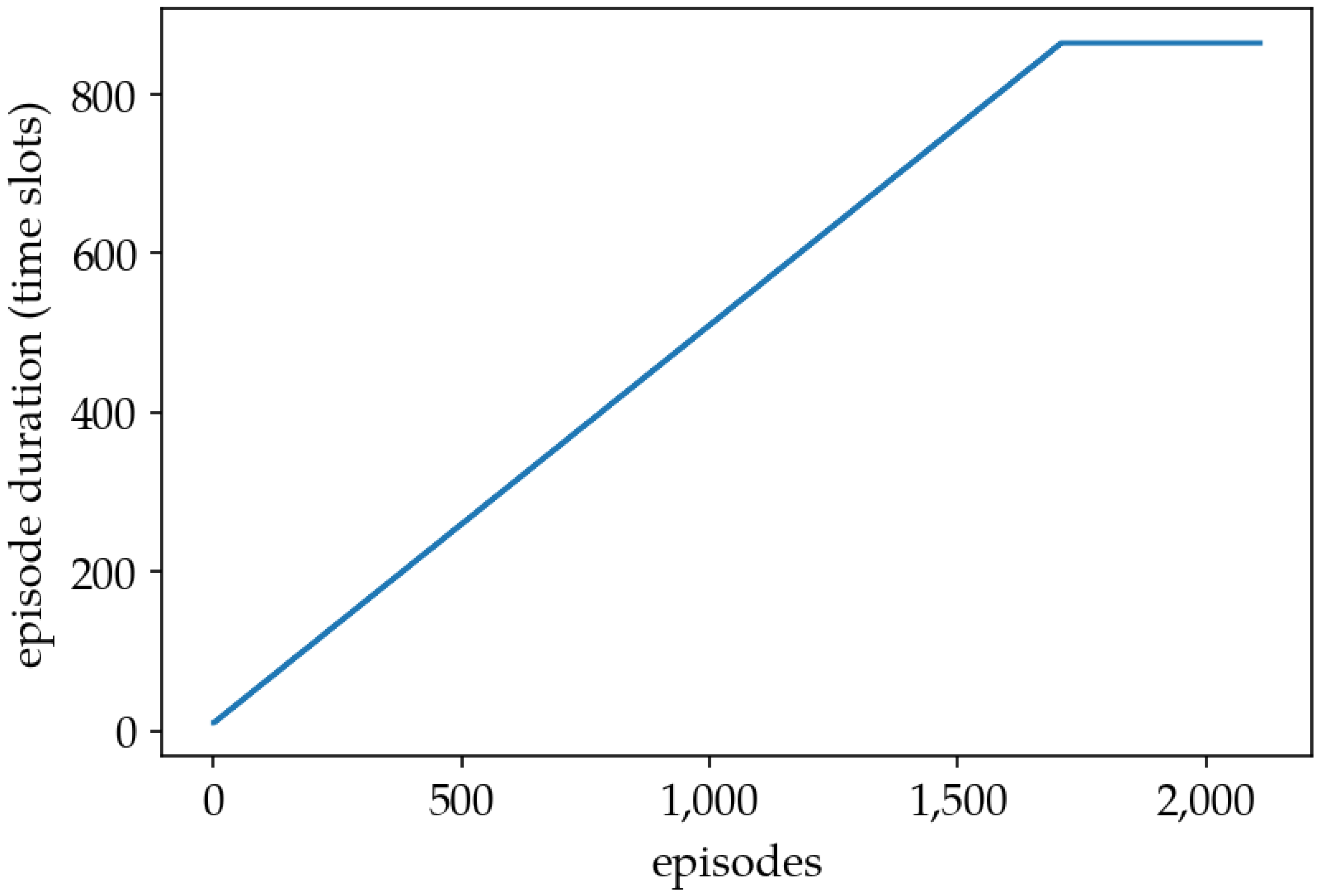
- Episode Duration
5. Results
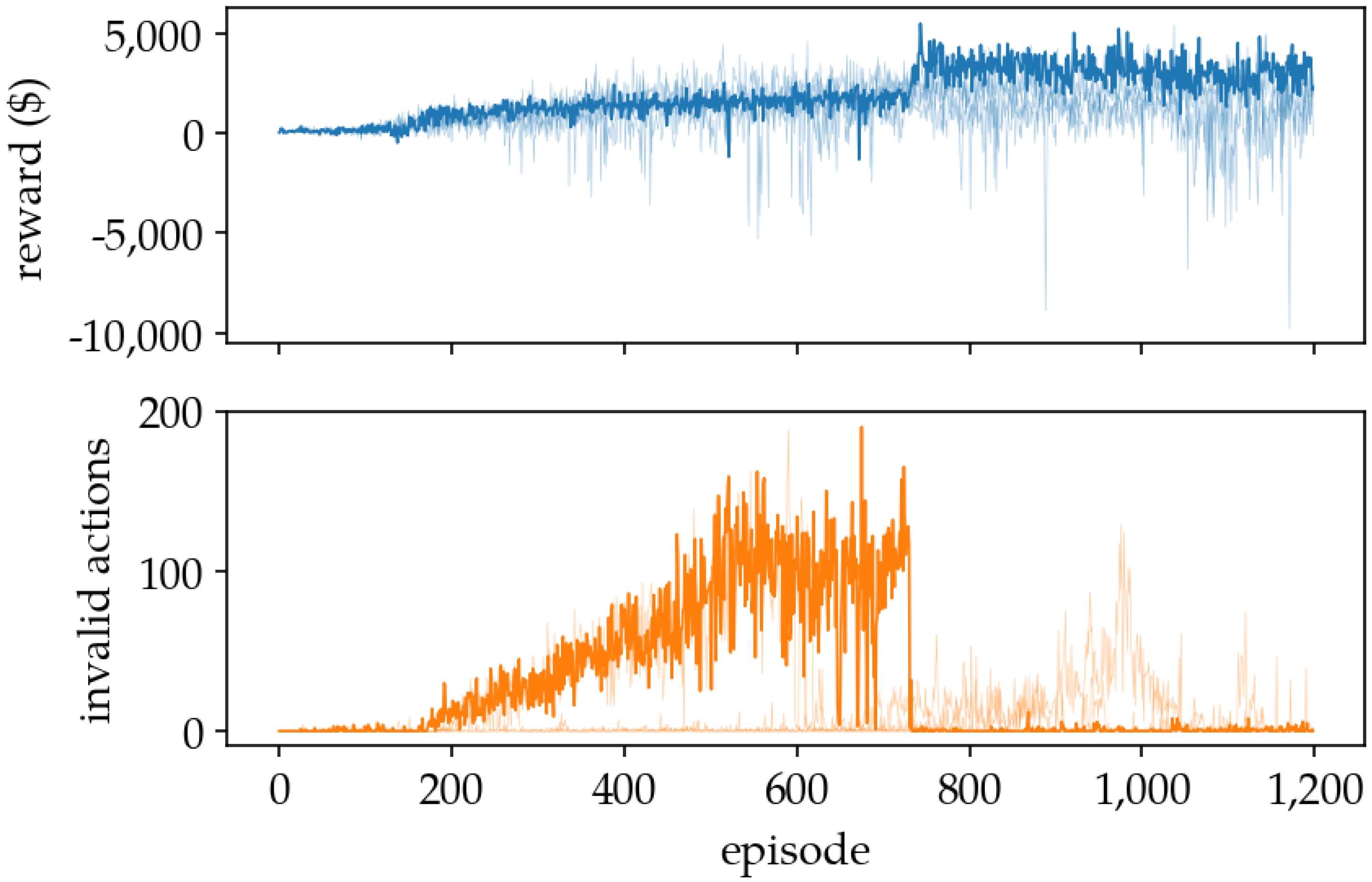
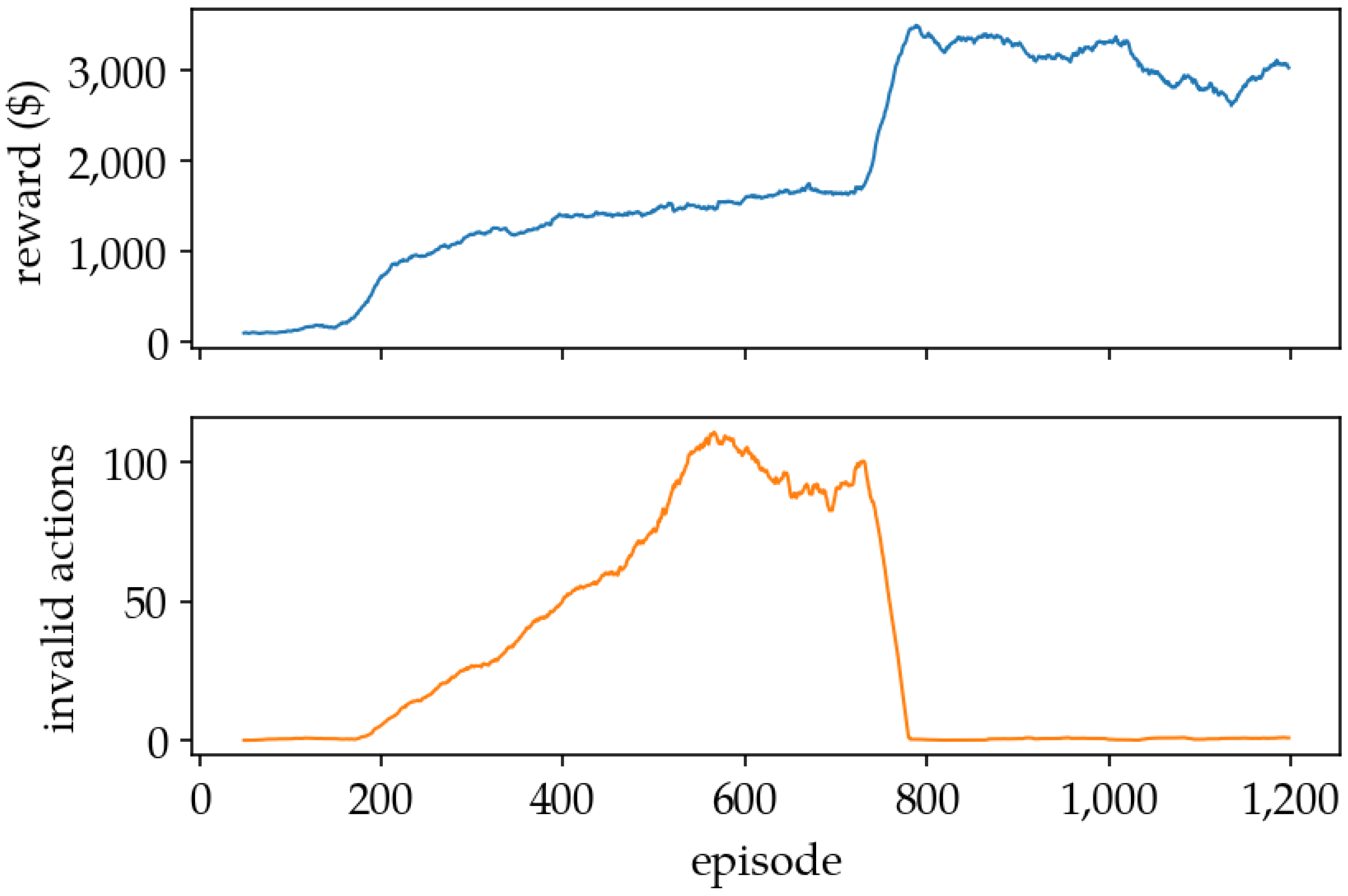
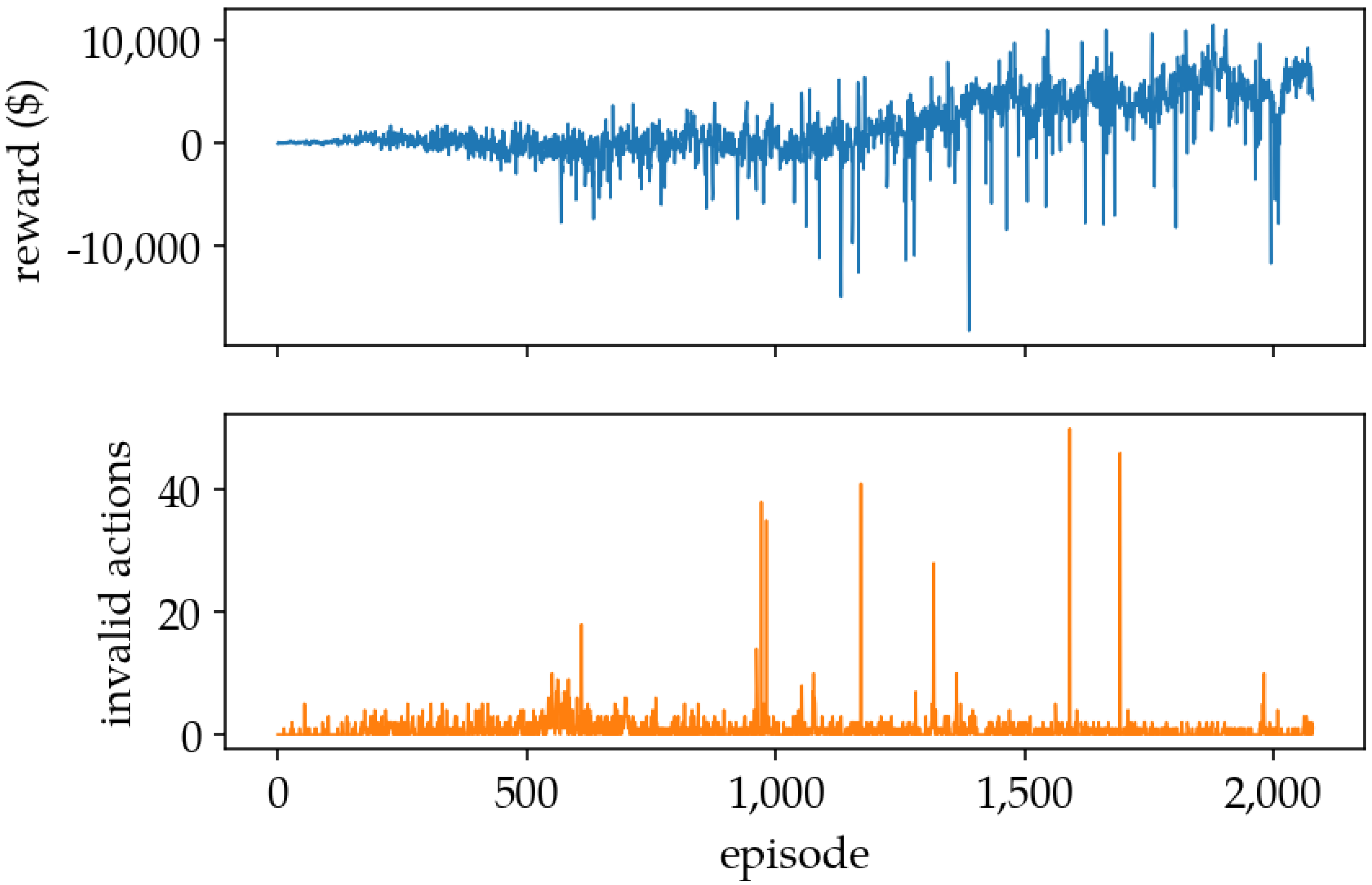
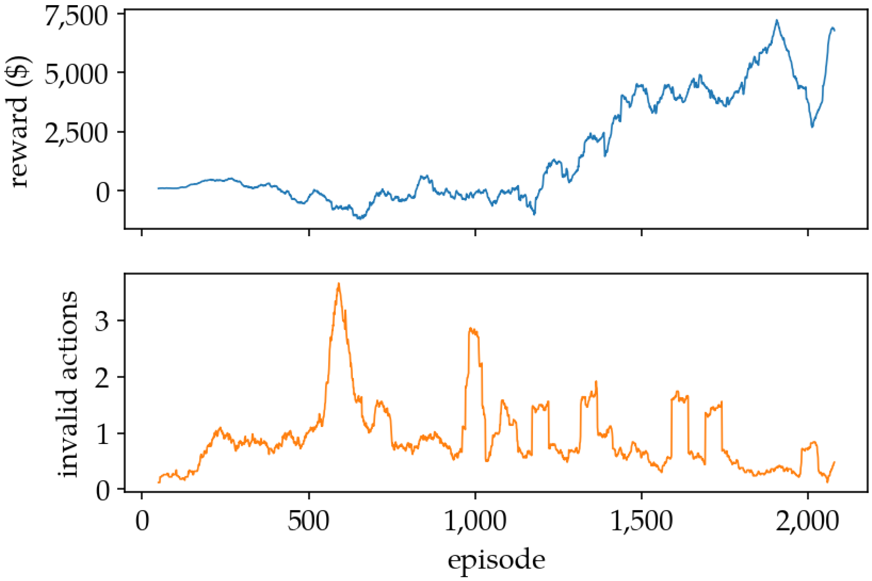
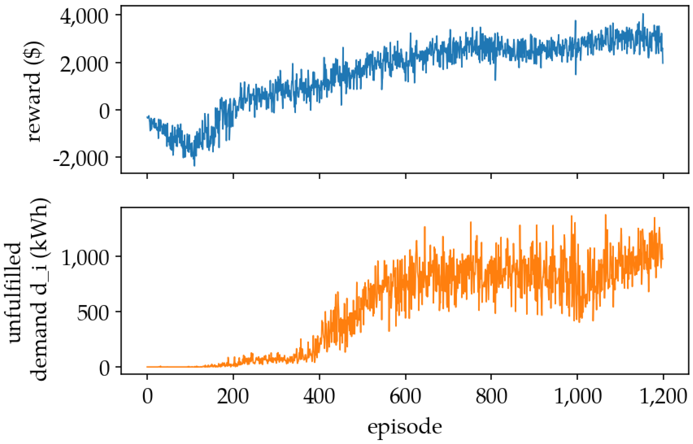
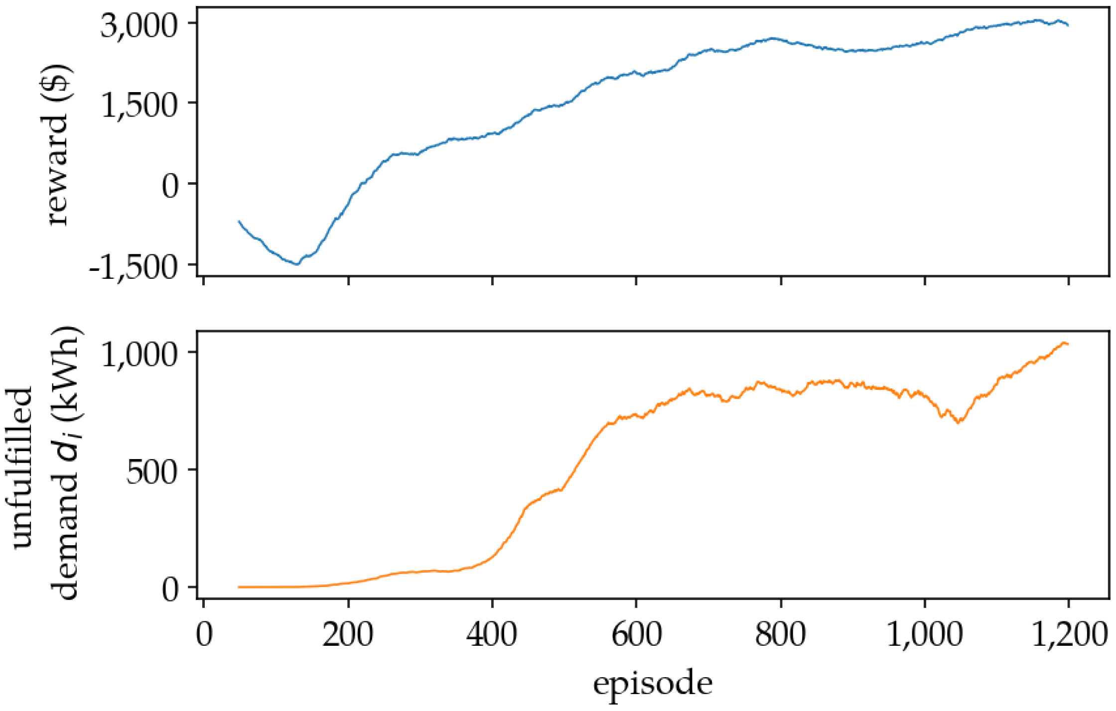
5.1. Training Results
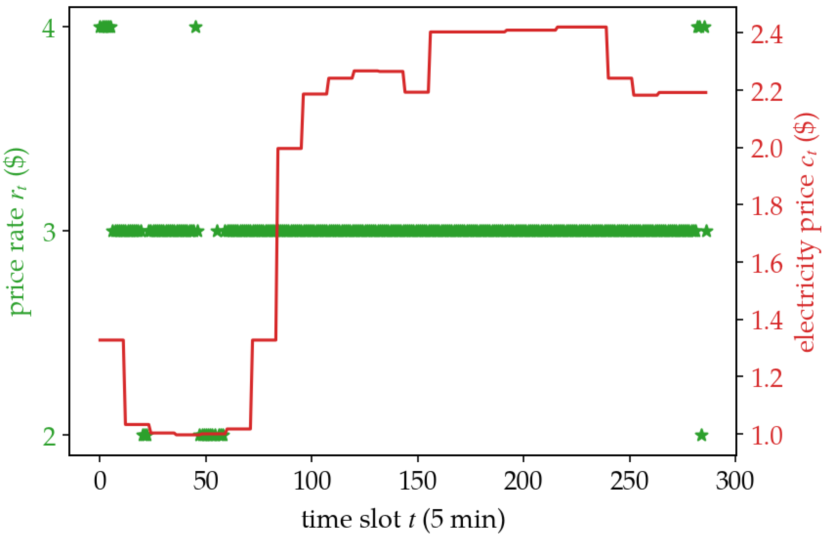
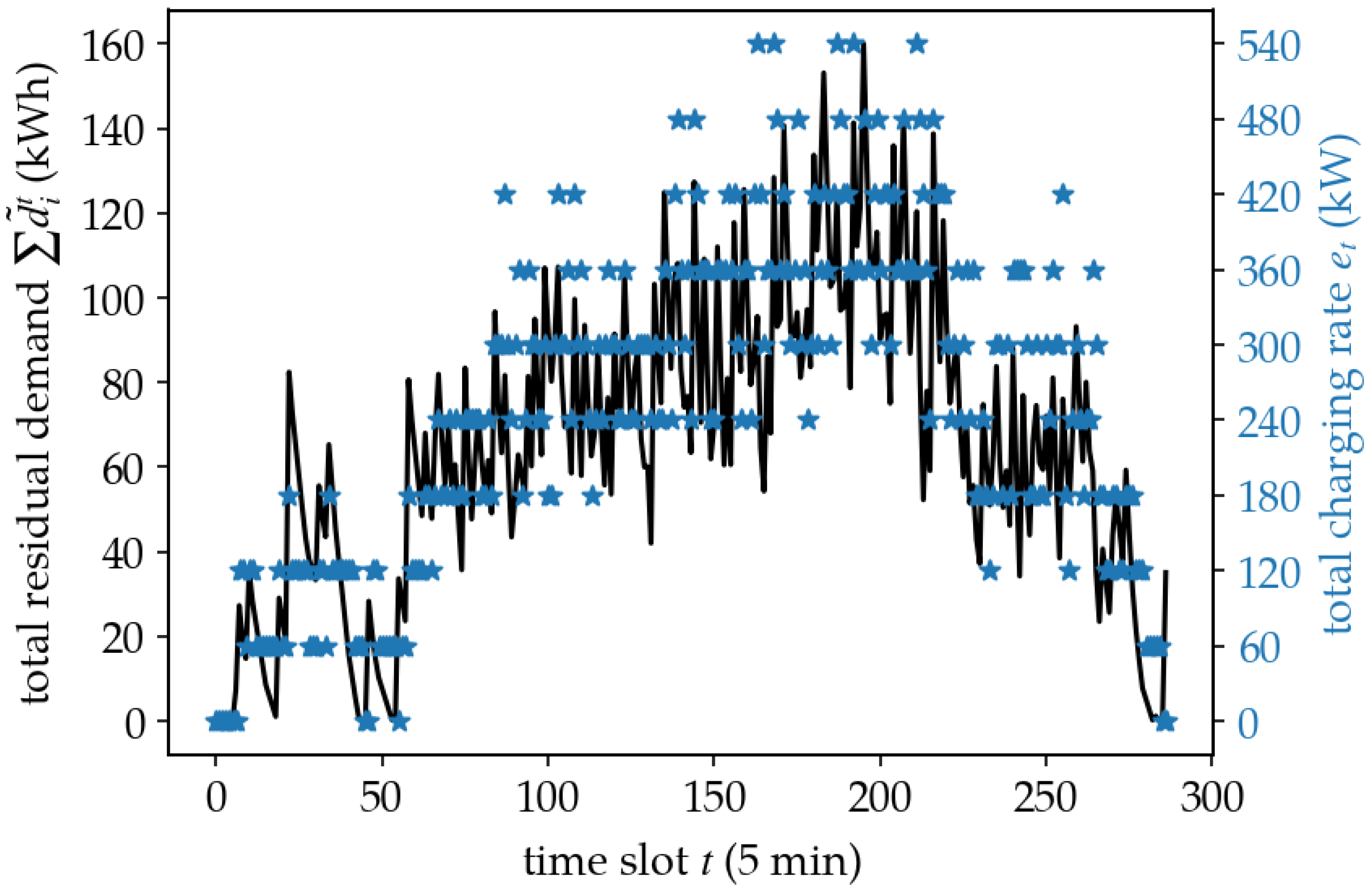
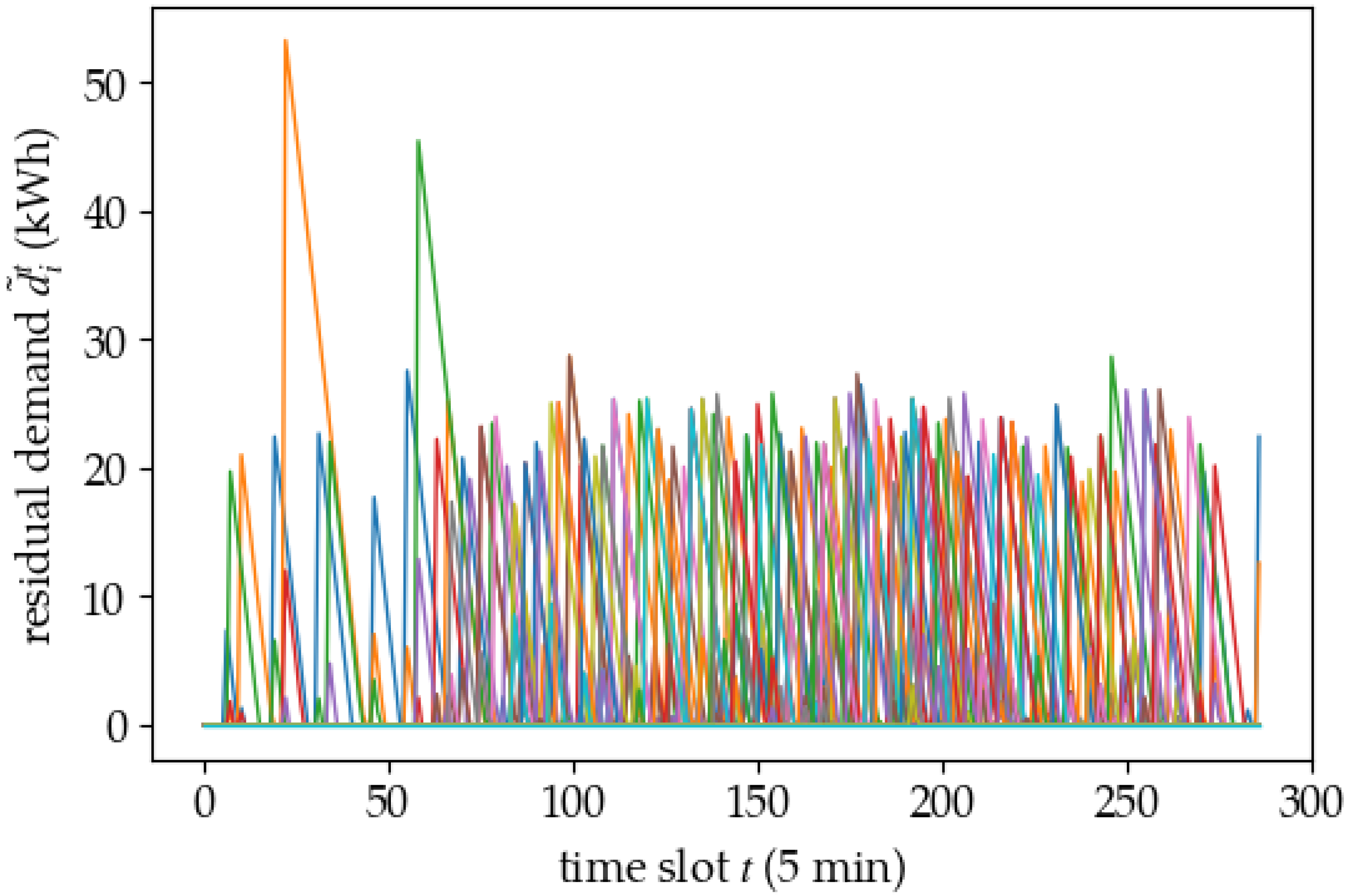
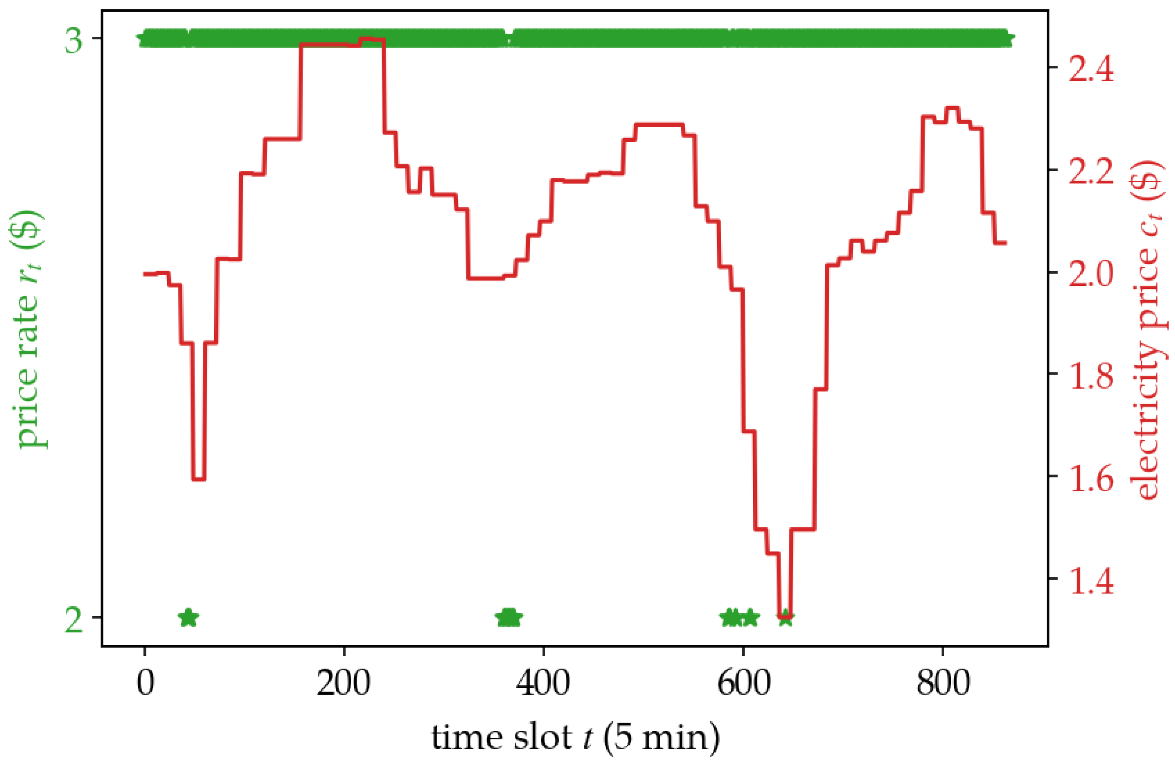
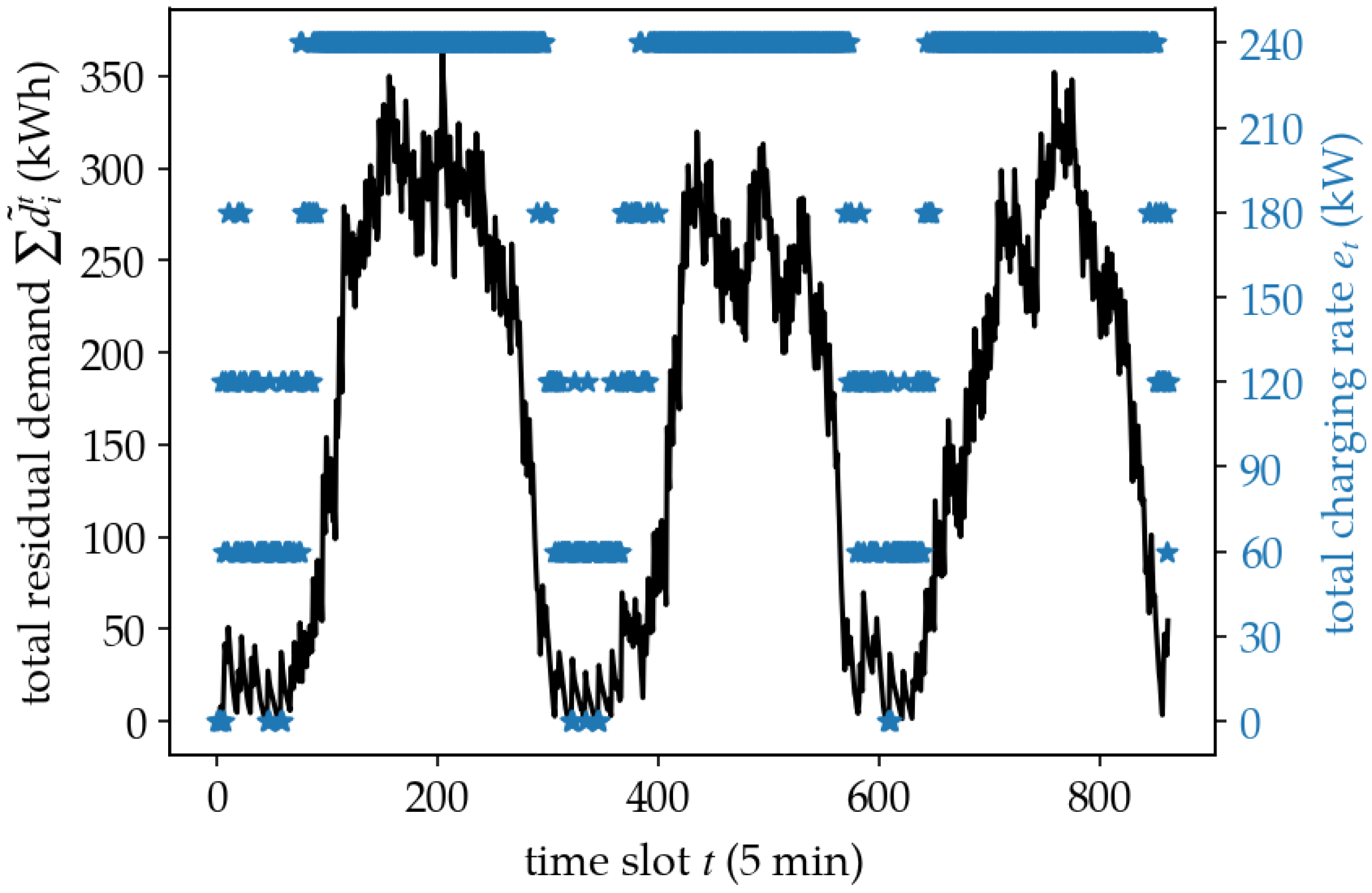
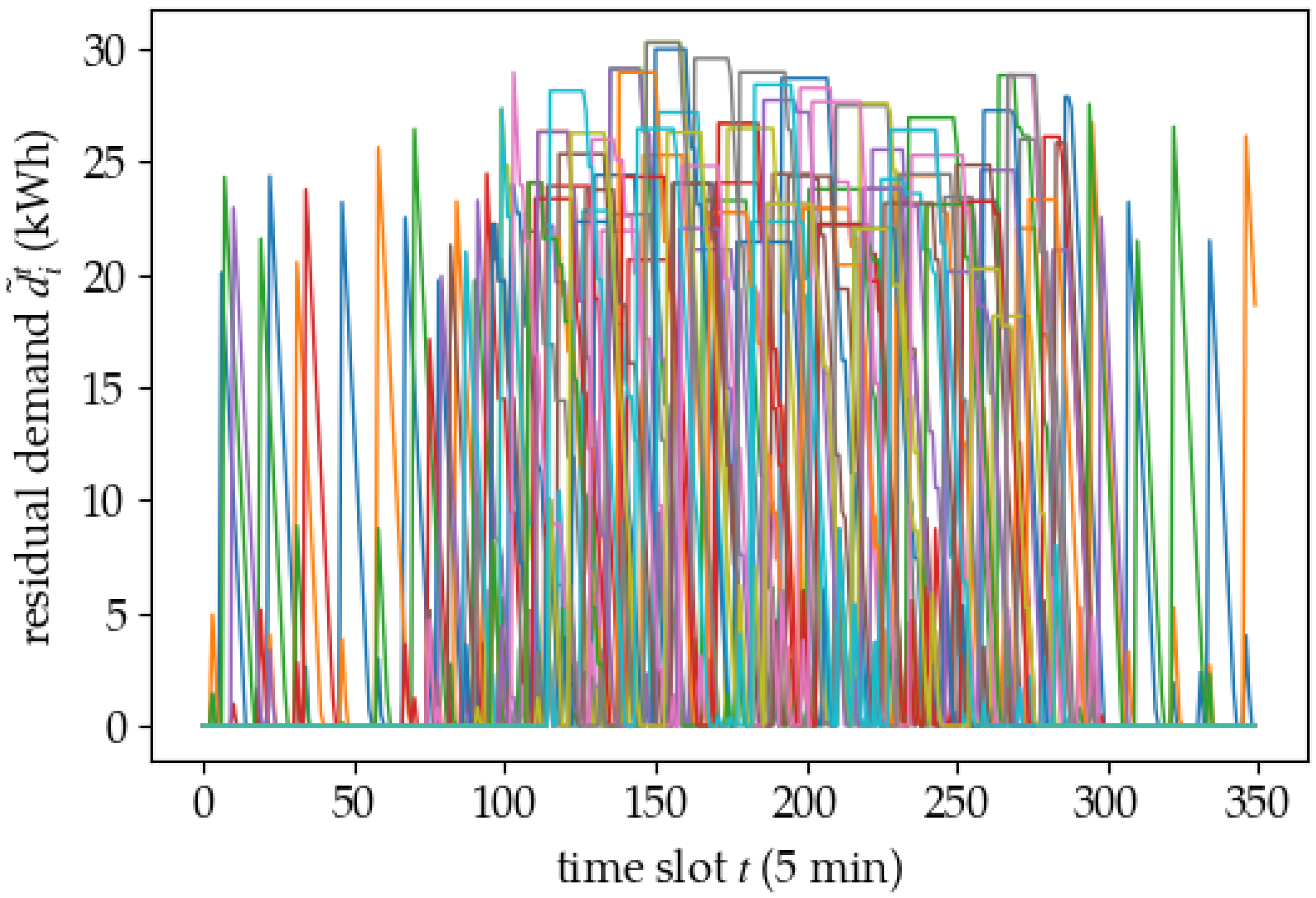
5.2. Policy Analysis
5.3. Case Study: Increasing Episode Time Horizon
5.4. Case Study: Removing Constraints
6. Conclusions
- As a first step, the technique of constraining the estimated charging rate could be incorporated into different DRL training algorithms that would operate on continuous action spaces, thereby lifting the need for discretizing scheduling and pricing actions.
- This work could serve as the basis for different formulations that consider more stakeholders, e.g., the grid operators and the corresponding constraints.
- Furthermore, the assumption was made that the total charging rate requested by the charging station is constrained only by the number of individual chargers. Consequently, potentially all parked EVs can be scheduled to charge during each slot; respecting additional constraints placed by the grid operator is an aspect that naturally arises as a potential future extension.
- In addition, more financial tools can be considered in modeling the relationship between different stakeholders.
- Finally, a more automated version of such a system can also be tailor-made for real-time EV detection, on a non-intrusive load monitoring (NILM) basis [31].
Author Contributions
Funding
Institutional Review Board Statement
Informed Consent Statement
Data Availability Statement
Conflicts of Interest
Nomenclature
| t | The time slot index |
| The length (duration) of each time slot | |
| The set of EVs that have arrived at the station at the beginning of time slot t | |
| The set of EVs that are already parked in the station before time slot t | |
| The set of EVs that require charging at time slot t | |
| The price rate announced to the customers at time slot t | |
| The arrival time of EV i | |
| The charging demand of EV i | |
| The maximum desired parking time of EV i | |
| The demand–response function of EV i | |
| The parameters of the demand–response function | |
| N | The total number of chargers in the station |
| The charging rate at which EV i will be charged during time slot t | |
| The maximum individual charging rate for every charger | |
| The total charging rate at time slot t | |
| The constrained total charging rate at time slot t | |
| The maximum total charging rate for the charging station | |
| The charging rate to energy conversion coefficient | |
| The electricity price that the charging station pays to the utility company | |
| The 4-tuple of elements of the Markov decision process | |
| The discount rate | |
| The residual charging demand for EV i at time slot t | |
| The residual parking time for EV i at time slot t | |
| The laxity of EV i at time slot t | |
| The relaxation coefficient | |
| The set of all available actions | |
| The set of discrete price rate levels | |
| L | The number of discrete price rate levels |
| The set of discrete charging rate levels | |
| K | The number of discrete charging rate levels |
| The probability of a random action of the -greedy policy | |
| The parameters of the -greedy policy |
References
- Azam, A.; Rafiq, M.; Shafique, M.; Yuan, J. Towards Achieving Environmental Sustainability: The Role of Nuclear Energy, Renewable Energy, and ICT in the Top-Five Carbon Emitting Countries. Front. Energy Res. 2021, 9, 804706. [Google Scholar] [CrossRef]
- Shafique, M.; Azam, A.; Rafiq, M.; Luo, X. Evaluating the Relationship between Freight Transport, Economic Prosperity, Urbanization, and CO2 Emissions: Evidence from Hong Kong, Singapore, and South Korea. Sustainability 2020, 12, 664. [Google Scholar] [CrossRef]
- Shafique, M.; Azam, A.; Rafiq, M.; Luo, X. Investigating the nexus among transport, economic growth and environmental degradation: Evidence from panel ARDL approach. Transp. Policy 2021, 109, 61–71. [Google Scholar] [CrossRef]
- Shafique, M.; Luo, X. Environmental life cycle assessment of battery electric vehicles from the current and future energy mix perspective. J. Environ. Manag. 2022, 303, 114050. [Google Scholar] [CrossRef]
- Yilmaz, M.; Krein, P.T. Review of the Impact of Vehicle-to-Grid Technologies on Distribution Systems and Utility Interfaces. IEEE Trans. Power Electron. 2013, 28, 5673–5689. [Google Scholar] [CrossRef]
- Shafique, M.; Azam, A.; Rafiq, M.; Luo, X. Life cycle assessment of electric vehicles and internal combustion engine vehicles: A case study of Hong Kong. Res. Transp. Econ. 2021, 101112. [Google Scholar] [CrossRef]
- International Energy Agency. Global EV Outlook. In Scaling-Up the Transition to Electric Mobility; IEA: London, UK, 2019. [Google Scholar]
- Statharas, S.; Moysoglou, Y.; Siskos, P.; Capros, P. Simulating the Evolution of Business Models for Electricity Recharging Infrastructure Development by 2030: A Case Study for Greece. Energies 2021, 14, 2345. [Google Scholar] [CrossRef]
- Almaghrebi, A.; Aljuheshi, F.; Rafaie, M.; James, K.; Alahmad, M. Data-Driven Charging Demand Prediction at Public Charging Stations Using Supervised Machine Learning Regression Methods. Energies 2020, 13, 4231. [Google Scholar] [CrossRef]
- Moghaddam, V.; Yazdani, A.; Wang, H.; Parlevliet, D.; Shahnia, F. An Online Reinforcement Learning Approach for Dynamic Pricing of Electric Vehicle Charging Stations. IEEE Access 2020, 8, 130305–130313. [Google Scholar] [CrossRef]
- Ghotge, R.; Snow, Y.; Farahani, S.; Lukszo, Z.; van Wijk, A. Optimized Scheduling of EV Charging in Solar Parking Lots for Local Peak Reduction under EV Demand Uncertainty. Energies 2020, 13, 1275. [Google Scholar] [CrossRef] [Green Version]
- He, Y.; Venkatesh, B.; Guan, L. Optimal Scheduling for Charging and Discharging of Electric Vehicles. IEEE Trans. Smart Grid 2012, 3, 1095–1105. [Google Scholar] [CrossRef]
- Tang, W.; Zhang, Y.J. A Model Predictive Control Approach for Low-Complexity Electric Vehicle Charging Scheduling: Optimality and Scalability. IEEE Trans. Power Syst. 2017, 32, 1050–1063. [Google Scholar] [CrossRef] [Green Version]
- Zhang, L.; Li, Y. Optimal Management for Parking-Lot Electric Vehicle Charging by Two-Stage Approximate Dynamic Programming. IEEE Trans. Smart Grid 2017, 8, 1722–1730. [Google Scholar] [CrossRef]
- Bellman, R. Dynamic Programming. Science 1966, 153, 34–37. [Google Scholar] [CrossRef] [PubMed]
- Sutton, R.S.; Barto, A.G. Reinforcement Learning: An Introduction, 2nd ed.; The MIT Press: Cambridge, MA, USA, 2018. [Google Scholar]
- Mnih, V.; Kavukcuoglu, K.; Silver, D.; Graves, A.; Antonoglou, I.; Wierstra, D.; Riedmiller, M.A. Playing Atari with Deep Reinforcement Learning. arXiv 2013, arXiv:1312.5602. [Google Scholar]
- Abdullah, H.M.; Gastli, A.; Ben-Brahim, L. Reinforcement Learning Based EV Charging Management Systems—A Review. IEEE Access 2021, 9, 41506–41531. [Google Scholar] [CrossRef]
- Lee, J.; Lee, E.; Kim, J. Electric Vehicle Charging and Discharging Algorithm Based on Reinforcement Learning with Data-Driven Approach in Dynamic Pricing Scheme. Energies 2020, 13, 1950. [Google Scholar] [CrossRef] [Green Version]
- Zhang, F.; Yang, Q.; An, D. CDDPG: A Deep-Reinforcement-Learning-Based Approach for Electric Vehicle Charging Control. IEEE Internet Things J. 2021, 8, 3075–3087. [Google Scholar] [CrossRef]
- Wan, Z.; Li, H.; He, H.; Prokhorov, D. Model-Free Real-Time EV Charging Scheduling Based on Deep Reinforcement Learning. IEEE Trans. Smart Grid 2019, 10, 5246–5257. [Google Scholar] [CrossRef]
- Wang, S.; Bi, S.; Zhang, Y.A. Reinforcement Learning for Real-Time Pricing and Scheduling Control in EV Charging Stations. IEEE Trans. Ind. Inform. 2021, 17, 849–859. [Google Scholar] [CrossRef]
- Chis, A.; Lunden, J.; Koivunen, V. Reinforcement Learning-Based Plug-in Electric Vehicle Charging with Forecasted Price. IEEE Trans. Veh. Technol. 2016, 66, 3674–3684. [Google Scholar] [CrossRef]
- Lucas, A.; Barranco, R.; Refa, N. EV Idle Time Estimation on Charging Infrastructure, Comparing Supervised Machine Learning Regressions. Energies 2019, 12, 269. [Google Scholar] [CrossRef] [Green Version]
- Deng, R.; Yang, Z.; Chow, M.Y.; Chen, J. A Survey on Demand Response in Smart Grids: Mathematical Models and Approaches. IEEE Trans. Ind. Inform. 2015, 11, 570–582. [Google Scholar] [CrossRef]
- Watkins, C.J.C.H. Learning from Delayed Rewards. Ph.D. Thesis, King’s College, Cambridge, UK, 1989. [Google Scholar]
- Pazis, J.; Lagoudakis, M.G. Reinforcement learning in multidimensional continuous action spaces. In Proceedings of the 2011 IEEE Symposium on Adaptive Dynamic Programming and Reinforcement Learning (ADPRL), Paris, France, 11–15 April 2011; pp. 97–104. [Google Scholar] [CrossRef]
- Mnih, V.; Kavukcuoglu, K.; Silver, D.; Rusu, A.A.; Veness, J.; Bellemare, M.G.; Graves, A.; Riedmiller, M.A.; Fidjeland, A.; Ostrovski, G.; et al. Human-level control through deep reinforcement learning. Nature 2015, 518, 529–533. [Google Scholar] [CrossRef] [PubMed]
- Exchange, K.P. System Marginal Price. Data Retrieved from Electric Power Statistics Information System. 2022. Available online: http://epsis.kpx.or.kr/epsisnew/selectEkmaSmpShdGrid.do?menuId=040202&locale=eng (accessed on 8 February 2022).
- Al-Saadi, M.; Olmos, J.; Saez-de Ibarra, A.; Van Mierlo, J.; Berecibar, M. Fast Charging Impact on the Lithium-Ion Batteries’ Lifetime and Cost-Effective Battery Sizing in Heavy-Duty Electric Vehicles Applications. Energies 2022, 15, 1278. [Google Scholar] [CrossRef]
- Athanasiadis, C.L.; Papadopoulos, T.A.; Doukas, D.I. Real-time non-intrusive load monitoring: A light-weight and scalable approach. Energy Build. 2021, 253, 111523. [Google Scholar] [CrossRef]


| EV Type | Standard Deviation | [kWh/$] | [kWh] | Parking Time |
|---|---|---|---|---|
| Emergent | 4.47 | −1 | 6 | 30 |
| Normal | 3.96 | −4 | 15 | 120 |
| Residential | 2.63 | −25 | 100 | 720 |
Publisher’s Note: MDPI stays neutral with regard to jurisdictional claims in published maps and institutional affiliations. |
© 2022 by the authors. Licensee MDPI, Basel, Switzerland. This article is an open access article distributed under the terms and conditions of the Creative Commons Attribution (CC BY) license (https://creativecommons.org/licenses/by/4.0/).
Share and Cite
Paraskevas, A.; Aletras, D.; Chrysopoulos, A.; Marinopoulos, A.; Doukas, D.I. Optimal Management for EV Charging Stations: A Win–Win Strategy for Different Stakeholders Using Constrained Deep Q-Learning. Energies 2022, 15, 2323. https://doi.org/10.3390/en15072323
Paraskevas A, Aletras D, Chrysopoulos A, Marinopoulos A, Doukas DI. Optimal Management for EV Charging Stations: A Win–Win Strategy for Different Stakeholders Using Constrained Deep Q-Learning. Energies. 2022; 15(7):2323. https://doi.org/10.3390/en15072323
Chicago/Turabian StyleParaskevas, Athanasios, Dimitrios Aletras, Antonios Chrysopoulos, Antonios Marinopoulos, and Dimitrios I. Doukas. 2022. "Optimal Management for EV Charging Stations: A Win–Win Strategy for Different Stakeholders Using Constrained Deep Q-Learning" Energies 15, no. 7: 2323. https://doi.org/10.3390/en15072323