
Regulated Two-Dimensional Deep Convolutional Neural Network-Based Power Quality Classifier for Microgrid

 ,
,  ,
,  and
and
Abstract
:1. Introduction
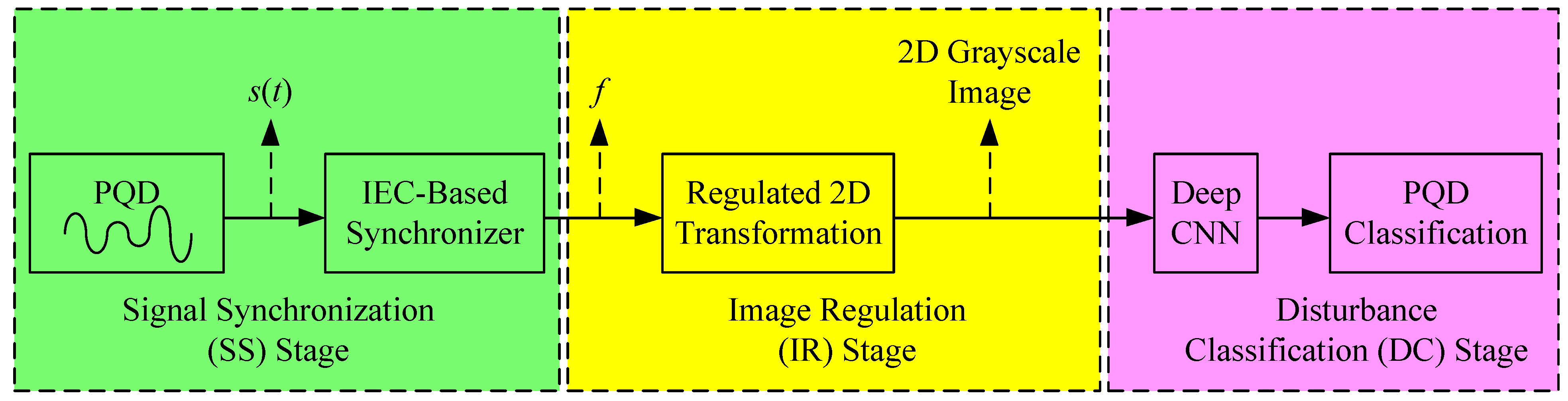
2. Proposed Regulated 2D Deep CNN-Based Power Quality Classifier
2.1. Mathematical Model of PQD
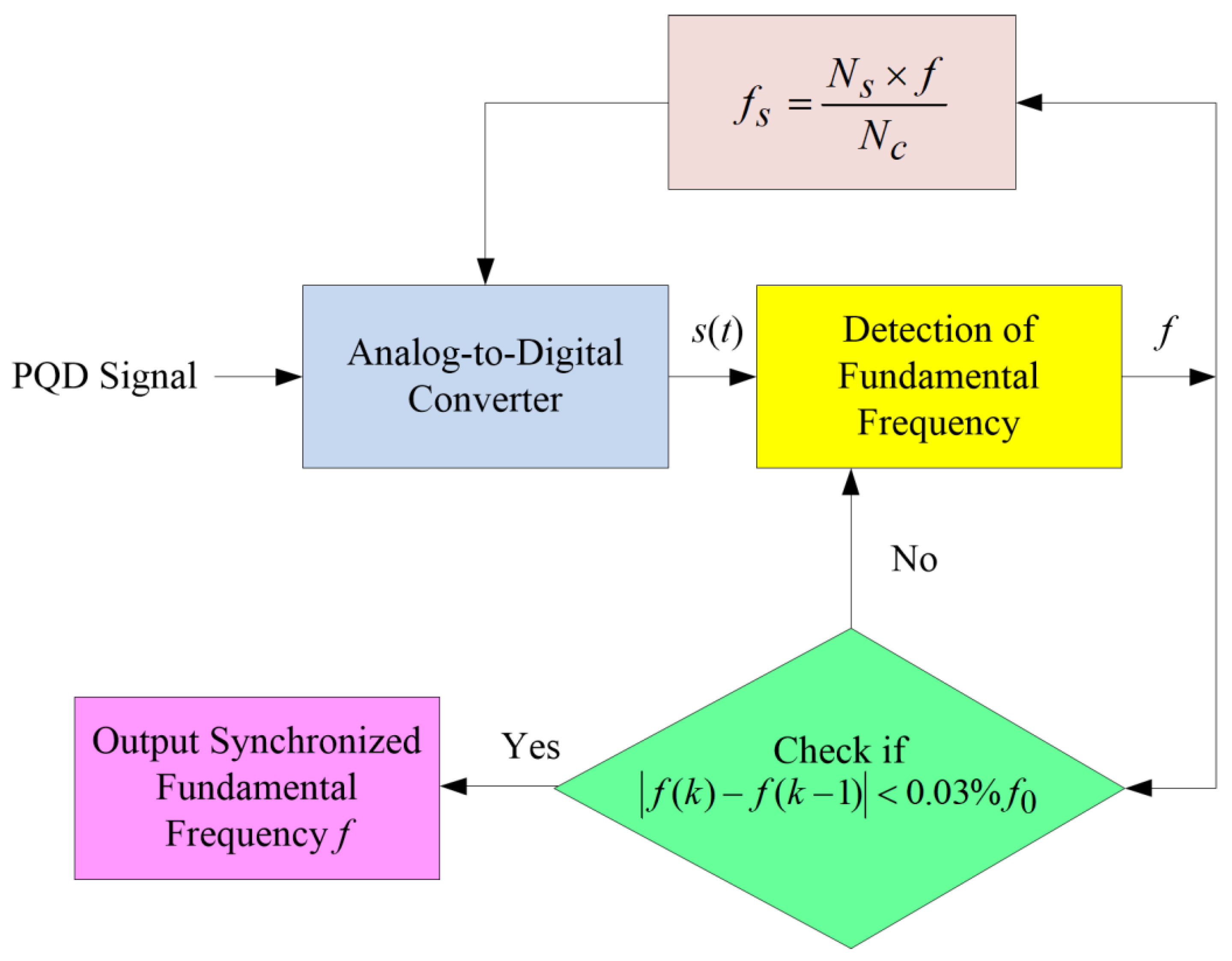
2.2. Signal Synchronization (SS)
2.3. Image Regulation (IR)
- Step 1.
- Determine the submatrix dimension.
- Step 2.
- Divide the PQD signal into multiple cycles.
- Step 3.
- Transform the divided cycles into submatrices.
- (1)
- Initialize all the elements of the lth submatrix Ml_x,y with Equation (9), where x and y are the row and column indices, respectively.
- (2)
- Determine the column index y of the lth submatrix Ml_x,y.The discrete-time index of the divided cycle is assigned as the column index to the submatrix, as listed in Equation (10), where y is the remainder of division between i and Ncol:
- (3)
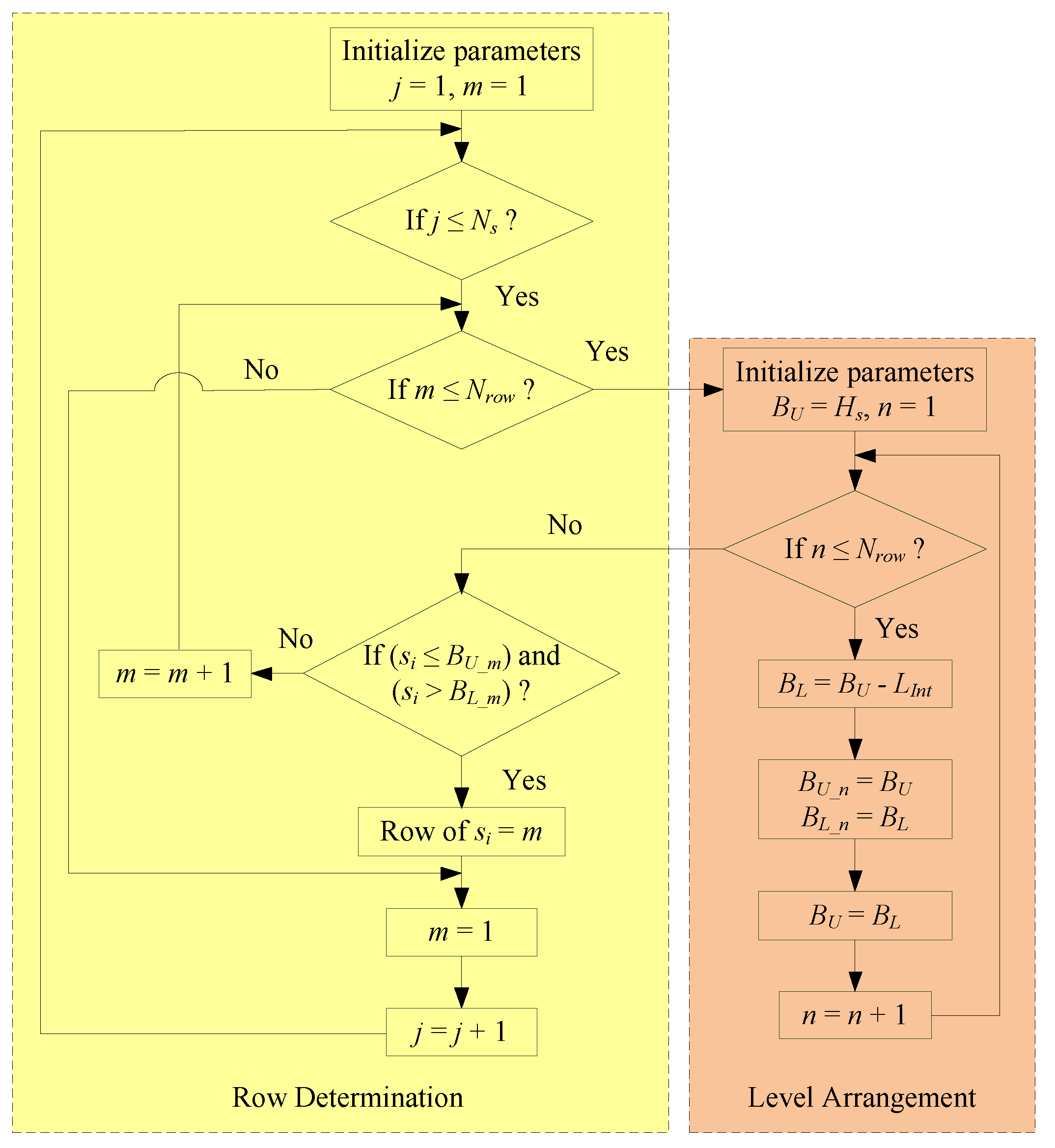
- Determine the row index x of the lth submatrix Ml_x,y.The process of row determination for each sampling point is displayed in Figure 3. The sampling values of the PQD signal are arranged into different levels. The number of levels should be the same as the number of rows, and the width of the level interval should be the same as well. The width of the level interval (LInt) is calculated with Equation (11):where Hs represents the highest sampling value and Ls represents the lowest sampling value from all the sampling values. In addition, the lower (BL) and upper (BU) boundaries are used to define the limits of levels, which can be obtained through the process in Figure 3. The order of levels is started from the highest sampling value as the first level, while the lowest sampling value is in the final level. According to the level arrangement in Figure 3, the row index, x, of each sampling point, si, can be obtained in Equation (12) by comparing the sampling value to all the levels:
- (4)
- Insert the sampling values of a divided cycle as the matrix elements with the obtained row and column indices.
- (5)
- Repeat the process to transform the rest of the cycles into the submatrices.
- Step 4.
- Merge the submatrices to form a regulated matrix.
- Step 5.
- Convert the regulated matrix to the 2D grayscale image.
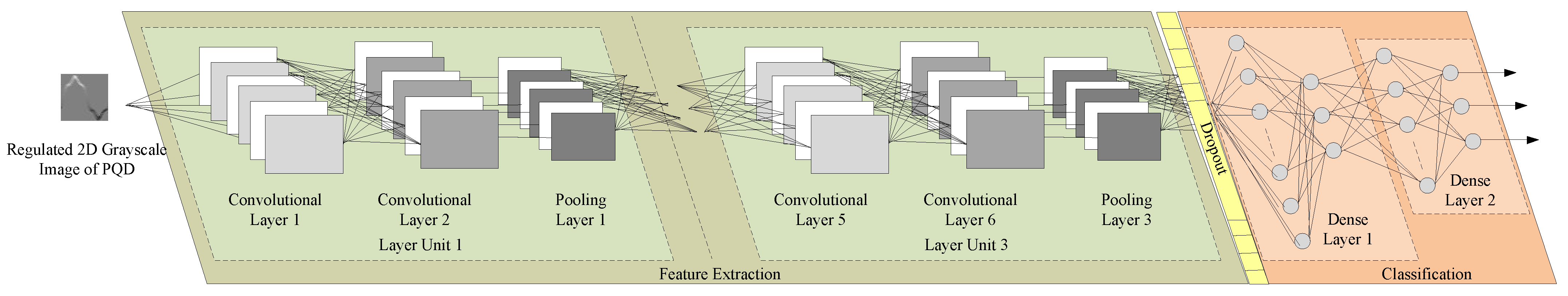
2.4. Disturbance Classification (DC)
2.5. Indices of Performance Evaluation
3. Results
3.1. Generation of Datasets and Regulated 2D Grayscale Image
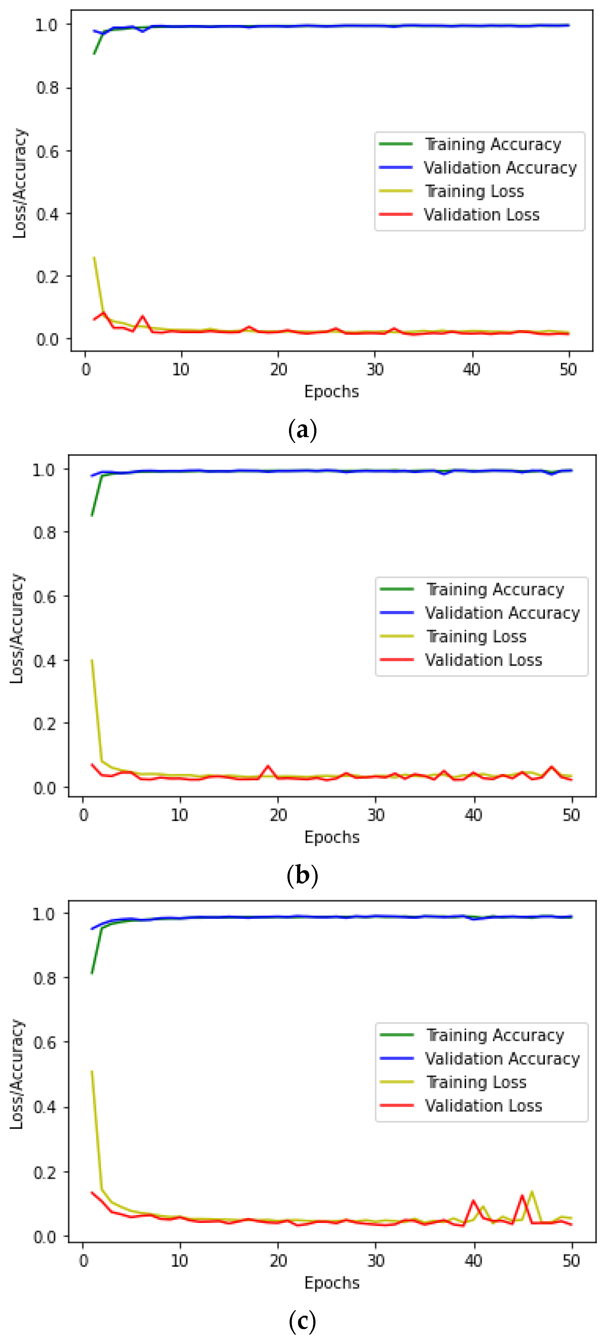
3.2. Results of Training and Evaluation Phases
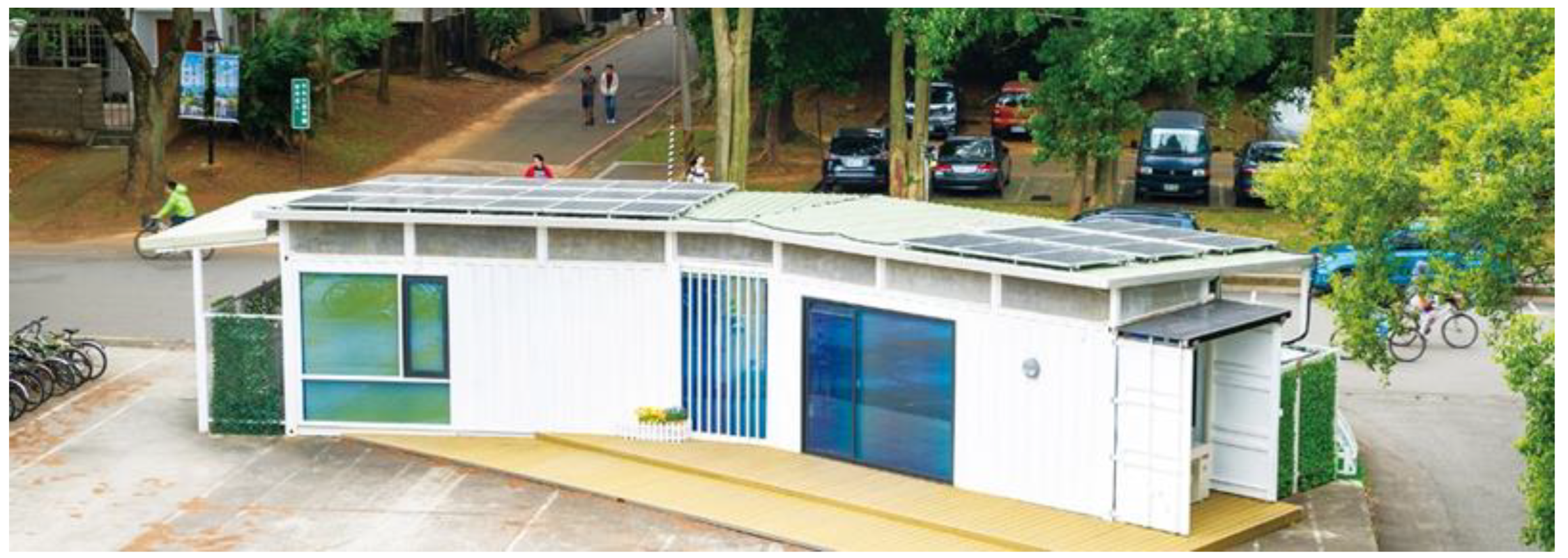
3.3. Field Verification
4. Conclusions
Author Contributions
Funding
Institutional Review Board Statement
Informed Consent Statement
Data Availability Statement
Acknowledgments
Conflicts of Interest
References
- Chen, C.I.; Chen, Y.C.; Chen, C.H.; Chang, Y.R. Voltage Regulation Using Recurrent Wavelet Fuzzy Neural Network-Based Dynamic Voltage Restorer. Energies 2020, 13, 6242. [Google Scholar] [CrossRef]
- Chen, C.I.; Lan, C.K.; Chen, Y.C.; Chen, C.H. Adaptive Frequency-Based Reference Compensation Current Control Strategy of Shunt Active Power Filter for Unbalanced Nonlinear Loads. Energies 2019, 12, 3080. [Google Scholar] [CrossRef] [Green Version]
- Sindi, H.; Nour, M.; Rawa, M.; Öztürk, Ş.; Polat, K. A Novel Hybrid Deep Learning Approach Including Combination of 1D Power Signals and 2D Signal Images for Power Quality Disturbance Classification. Expert Syst. Appl. 2021, 174, 114785. [Google Scholar] [CrossRef]
- Wang, S.; Chen, H. A Novel Deep Learning Method for the Classification of Power Quality Disturbances Using Deep Convolutional Neural Network. Appl. Energy 2019, 235, 1126–1140. [Google Scholar] [CrossRef]
- Shen, Y.; Abubakar, M.; Liu, H.; Hussain, F. Power Quality Disturbance Monitoring and Classification Based on Improved PCA and Convolution Neural Network for Wind-Grid Distribution Systems. Energies 2019, 12, 1280. [Google Scholar] [CrossRef] [Green Version]
- Aggarwal, A.; Das, N.; Arora, M.; Tripathi, M.M. A Novel Hybrid Architecture for Classification of Power Quality Disturbances. In Proceedings of the 2019 6th International Conference on Control, Decision and Information Technologies (CoDIT), Paris, France, 23–26 April 2019; pp. 1829–1834. [Google Scholar]
- Mohan, N.; Soman, K.P.; Vinayakumar, R. Deep Power: Deep Learning Architectures for Power Quality Disturbances Classification. In Proceedings of the 2017 International Conference on Technological Advancements in Power and Energy (TAP Energy), Kollam, India, 21–23 December 2017; pp. 1–6. [Google Scholar]
- Wang, J.; Xu, Z.; Che, Y. Power Quality Disturbance Classification Based on Compressed Sensing and Deep Convolutional Neural Networks. IEEE Access. 2019, 7, 78336–78346. [Google Scholar] [CrossRef]
- Öztürk, Ş.; Akdemir, B. Cell-Type Based Semantic Segmentation of Histopathological Images Using Deep Convolutional Neural Networks. Int. J. Imaging Syst. Technol. 2019, 29, 234–246. [Google Scholar] [CrossRef]
- Liu, H.; Hussain, F.; Shen, Y.; Arif, S.; Nazir, A.; Abubakar, M. Complex Power Quality Disturbances Classification via Curvelet Transform and Deep Learning. Electr. Power Syst. Res. 2018, 163, 1–9. [Google Scholar] [CrossRef]
- Zhu, R.; Gong, X.; Hu, S.; Wang, Y. Power Quality Disturbances Classification via Fully-Convolutional Siamese Network and k-Nearest Neighbor. Energies 2019, 12, 4732. [Google Scholar] [CrossRef] [Green Version]
- Bagheri, A.; Bollen, M.H.J.; Gu, I.Y.H. Improved Characterization of Multi-Stage Voltage Dips Based on the Space Phasor Model. Electr. Power Syst. Res. 2018, 154, 319–328. [Google Scholar] [CrossRef]
- Bagheri, A.; Gu, I.Y.H.; Bollen, M.H.J.; Balouji, E. A Robust Transform-Domain Deep Convolutional Network for Voltage Dip Classification. IEEE Trans. Power Deliv. 2018, 33, 2794–2802. [Google Scholar] [CrossRef] [Green Version]
- Xiao, F.; Lu, T.; Wu, M.; Ai, Q. Maximal Overlap Discrete Wavelet Transform and Deep Learning for Robust Denoising and Detection of Power Quality Disturbance. IET Gener. Transm. Distrib. 2020, 14, 140–147. [Google Scholar] [CrossRef]
- Karasu, S.; Saraç, Z. Investigation of Power Quality Disturbances by Using 2D Discrete Orthonormal S-Transform, Machine Learning and Multi-Objective Evolutionary Algorithms. Swarm Evol. Comput. 2019, 44, 1060–1072. [Google Scholar] [CrossRef]
- Karasu, S.; Saraç, Z. Classification of Power Quality Disturbances by 2D-Riesz Transform, Multi-Objective Grey Wolf Optimizer and Machine Learning Methods. Digit. Signal Process. 2020, 101, 102711. [Google Scholar] [CrossRef]
- Zheng, Z.; Qi, L.; Wang, H.; Pan, A.; Zhou, J. Recognition Method of Voltage Sag Causes Based on Two-Dimensional Transform and Deep Learning Hybrid Model. IET Power Electron. 2020, 13, 168–177. [Google Scholar] [CrossRef]
- IEEE Recommended Practice for Monitoring Electric Power Quality; IEEE Std.: New York, NY, USA, 2019; pp. 1159–2019.
- IEC 61000-4-7; Testing and Measurement Techniques—General Guide on Harmonics and Interharmonics Measurements and Instrumentation, for Power Supply Systems and Equipment Connected Thereto. IEC Std.: Geneva, Switzerland, 2009.
- Chang, G.W.; Chen, C.I.; Liang, Q.W. A Two-Stage ADALINE for Harmonics and Interharmonics Measurement. IEEE Trans. Ind. Electron. 2009, 56, 2220–2228. [Google Scholar] [CrossRef]
- Cai, K.; Cao, W.; Aarniovuori, L.; Pang, H.; Lin, Y.; Li, G. Classification of Power Quality Disturbances Using Wigner-Ville Distribution and Deep Convolutional Neural Networks. IEEE Access 2019, 7, 119099–119109. [Google Scholar] [CrossRef]
- Xu, J.; Zhang, Y.; Miao, D. Three-Way Confusion Matrix for Classification: A Measure Driven View. Inf. Sci. 2020, 507, 772–794. [Google Scholar] [CrossRef]
- Tharwat, A. Classification Assessment Methods. Appl. Comput. Inform. 2021, 17, 168–192. [Google Scholar] [CrossRef]
- Li, H.; Chen, M.; Yang, B.; Blaabjerg, F.; Xu, D. Fast Fault Protection Based on Direction of Fault Current for the High-Surety Power-Supply System. IEEE Trans. Power Electron. 2019, 34, 5787–5802. [Google Scholar] [CrossRef] [Green Version]
- Dash, P.K.; Mishra, S.; Salama, M.M.A.; Liew, A.C. Classification of Power System Disturbances Using a Fuzzy Expert System and a Fourier Linear Combiner. IEEE Trans. Power Deliv. 2010, 15, 472–477. [Google Scholar] [CrossRef] [Green Version]
- Kumar, R.; Singh, B.; Shahani, D.T.; Chandra, A.; Al-Haddad, K. Recognition of Power-Quality Disturbances Using S-Transform-Based ANN Classifier and Rule-Based Decision Tree. IEEE Trans. Ind. Appl. 2015, 51, 1249–1258. [Google Scholar] [CrossRef]
- Chen, C.I.; Lan, C.K.; Chen, Y.C.; Chen, C.H.; Chang, Y.R. Wavelet Energy Fuzzy Neural Network-Based Fault Protection System for Microgrid. Energies 2020, 13, 1007. [Google Scholar] [CrossRef] [Green Version]


| PQD | Category | Mathematical Model | Parameter Constraints |
|---|---|---|---|
| Normal | C01 | ||
| Sag | C02 | ||
| Swell | C03 | ||
| Interruption | C04 | ||
| Harmonics | C05 | ||
| Flicker | C06 | ||
| Transient oscillation | C07 | ||
| Periodic notch | C08 | ||
| Sag with harmonics | C09 | ||
| Swell with harmonics | C10 | ||
| Interruption with harmonics | C11 | ||
| Flicker with harmonics | C12 | ||
| Flicker with sag | C13 | ||
| Flicker with swell | C14 |
| Layer | Parameters |
|---|---|
| Convolution 1 | Number of kernal filters = 32, Kernal size = 5 × 5, Activation function: ReLU |
| Convolution 2 | Number of kernal filters = 32, Kernal size = 5 × 5, Activation function: ReLU |
| Pooling 1 | Max pooling, Size = 2 × 2, Step: 2 |
| Convolution 3 | Number of kernal filters = 32, Kernal size = 5 × 5, Activation function: ReLU |
| Convolution 4 | Number of kernal filters = 32, Kernal size = 5 × 5, Activation function: ReLU |
| Pooling 2 | Max pooling, Size = 2 × 2, Step: 2 |
| Convolution 5 | Number of kernal filters = 32, Kernal size = 5 × 5, Activation function: ReLU |
| Convolution 6 | Number of kernal filters = 32, Kernal size = 5 × 5, Activation function: ReLU |
| Pooling 3 | Max pooling, Size = 2 × 2, Step: 2 |
| Dense 1 | Number of neurons: 128, Activation function: ReLU |
| Dense 2 | Number of neurons: 14, Activation function: softmax |
| PQD Type | PQD Signal | 2D Grayscale Image | PQD Type | PQD Signal | 2D Grayscale Image |
|---|---|---|---|---|---|
| Normal |  |  | Sag wit harmonics |  |  |
| Flicker |  |  | Swell with harmonics |  |  |
| Harmonics |  |  | Interruption with harmonics |  |  |
| Interruption |  |  | Flicker with harmonics |  |  |
| Notch |  |  | Flicker with sag |  |  |
| Sag |  |  | Flicker with swell |  |  |
| Swell |  |  | Transient |  |  |
| Models | Training Accuracy (%) | Validation Accuracy (%) |
|---|---|---|
| Proposed Method | 99.25 | 99.46 |
| Karasu’s Method in [15,16] | 98.69 | 98.94 |
| Zheng’s Method in [17] | 97.98 | 98.43 |
| Category | C01 | C02 | C03 | C04 | C05 | C06 | C07 | C08 | C09 | C10 | C11 | C12 | C13 | C14 |
|---|---|---|---|---|---|---|---|---|---|---|---|---|---|---|
| C01 | 998 | 0 | 0 | 2 | 0 | 0 | 0 | 0 | 0 | 0 | 0 | 0 | 0 | 0 |
| C02 | 0 | 988 | 0 | 12 | 0 | 0 | 0 | 0 | 0 | 0 | 0 | 0 | 0 | 0 |
| C03 | 0 | 0 | 998 | 0 | 0 | 0 | 2 | 0 | 0 | 0 | 0 | 0 | 0 | 0 |
| C04 | 0 | 2 | 0 | 998 | 0 | 0 | 0 | 0 | 0 | 0 | 0 | 0 | 0 | 0 |
| C05 | 0 | 0 | 0 | 0 | 1000 | 0 | 0 | 0 | 0 | 0 | 0 | 0 | 0 | 0 |
| C06 | 0 | 0 | 0 | 0 | 0 | 1000 | 0 | 0 | 0 | 0 | 0 | 0 | 0 | 0 |
| C07 | 0 | 0 | 0 | 0 | 0 | 0 | 1000 | 0 | 0 | 0 | 0 | 0 | 0 | 0 |
| C08 | 0 | 0 | 0 | 0 | 0 | 0 | 0 | 1000 | 0 | 0 | 0 | 0 | 0 | 0 |
| C09 | 0 | 0 | 0 | 0 | 0 | 0 | 0 | 0 | 992 | 0 | 8 | 0 | 0 | 0 |
| C10 | 0 | 0 | 0 | 0 | 0 | 0 | 0 | 0 | 0 | 1000 | 0 | 0 | 0 | 0 |
| C11 | 0 | 0 | 0 | 0 | 0 | 0 | 0 | 0 | 0 | 0 | 1000 | 0 | 0 | 0 |
| C12 | 0 | 0 | 0 | 0 | 0 | 0 | 0 | 0 | 0 | 0 | 0 | 1000 | 0 | 0 |
| C13 | 0 | 0 | 0 | 0 | 0 | 0 | 0 | 0 | 0 | 0 | 0 | 0 | 1000 | 0 |
| C14 | 0 | 0 | 0 | 0 | 0 | 0 | 0 | 0 | 0 | 0 | 0 | 0 | 0 | 1000 |
| Category | C01 | C02 | C03 | C04 | C05 | C06 | C07 | C08 | C09 | C10 | C11 | C12 | C13 | C14 |
|---|---|---|---|---|---|---|---|---|---|---|---|---|---|---|
| C01 | 994 | 0 | 0 | 0 | 0 | 0 | 6 | 0 | 0 | 0 | 0 | 0 | 0 | 0 |
| C02 | 28 | 960 | 0 | 12 | 0 | 0 | 0 | 0 | 0 | 0 | 0 | 0 | 0 | 0 |
| C03 | 0 | 0 | 998 | 0 | 0 | 0 | 2 | 0 | 0 | 0 | 0 | 0 | 0 | 0 |
| C04 | 0 | 20 | 0 | 980 | 0 | 0 | 0 | 0 | 0 | 0 | 0 | 0 | 0 | 0 |
| C05 | 0 | 0 | 0 | 0 | 1000 | 0 | 0 | 0 | 0 | 0 | 0 | 0 | 0 | 0 |
| C06 | 0 | 0 | 0 | 0 | 0 | 1000 | 0 | 0 | 0 | 0 | 0 | 0 | 0 | 0 |
| C07 | 4 | 4 | 4 | 0 | 0 | 0 | 986 | 2 | 0 | 0 | 0 | 0 | 0 | 0 |
| C08 | 2 | 0 | 0 | 0 | 0 | 0 | 0 | 998 | 0 | 0 | 0 | 0 | 0 | 0 |
| C09 | 0 | 0 | 0 | 0 | 0 | 0 | 0 | 0 | 980 | 0 | 20 | 0 | 0 | 0 |
| C10 | 0 | 0 | 0 | 0 | 0 | 0 | 0 | 0 | 0 | 1000 | 0 | 0 | 0 | 0 |
| C11 | 0 | 0 | 0 | 0 | 0 | 0 | 0 | 0 | 8 | 0 | 992 | 0 | 0 | 0 |
| C12 | 0 | 0 | 0 | 0 | 0 | 0 | 0 | 0 | 0 | 0 | 0 | 1000 | 0 | 0 |
| C13 | 0 | 0 | 0 | 0 | 0 | 0 | 0 | 0 | 0 | 0 | 0 | 0 | 1000 | 0 |
| C14 | 0 | 0 | 0 | 0 | 0 | 0 | 0 | 0 | 0 | 0 | 0 | 0 | 2 | 998 |
| Category | C01 | C02 | C03 | C04 | C05 | C06 | C07 | C08 | C09 | C10 | C11 | C12 | C13 | C14 |
|---|---|---|---|---|---|---|---|---|---|---|---|---|---|---|
| C01 | 998 | 0 | 0 | 0 | 0 | 0 | 0 | 2 | 0 | 0 | 0 | 0 | 0 | 0 |
| C02 | 32 | 926 | 0 | 42 | 0 | 0 | 0 | 0 | 0 | 0 | 0 | 0 | 0 | 0 |
| C03 | 0 | 0 | 1000 | 0 | 0 | 0 | 0 | 0 | 0 | 0 | 0 | 0 | 0 | 0 |
| C04 | 0 | 10 | 0 | 990 | 0 | 0 | 0 | 0 | 0 | 0 | 0 | 0 | 0 | 0 |
| C05 | 0 | 0 | 0 | 0 | 1000 | 0 | 0 | 0 | 0 | 0 | 0 | 0 | 0 | 0 |
| C06 | 0 | 0 | 0 | 0 | 0 | 1000 | 0 | 0 | 0 | 0 | 0 | 0 | 0 | 0 |
| C07 | 16 | 4 | 0 | 2 | 0 | 0 | 974 | 4 | 0 | 0 | 0 | 0 | 0 | 0 |
| C08 | 4 | 0 | 0 | 0 | 0 | 0 | 0 | 996 | 0 | 0 | 0 | 0 | 0 | 0 |
| C09 | 0 | 0 | 0 | 0 | 0 | 0 | 0 | 0 | 958 | 0 | 42 | 0 | 0 | 0 |
| C10 | 0 | 0 | 0 | 0 | 0 | 0 | 0 | 0 | 0 | 1000 | 0 | 0 | 0 | 0 |
| C11 | 0 | 0 | 0 | 0 | 0 | 0 | 0 | 0 | 6 | 0 | 994 | 0 | 0 | 0 |
| C12 | 0 | 0 | 0 | 0 | 0 | 0 | 0 | 0 | 2 | 0 | 0 | 998 | 0 | 0 |
| C13 | 0 | 0 | 0 | 0 | 0 | 0 | 0 | 0 | 0 | 0 | 0 | 0 | 1000 | 0 |
| C14 | 0 | 0 | 0 | 0 | 0 | 0 | 0 | 0 | 0 | 0 | 0 | 0 | 2 | 998 |
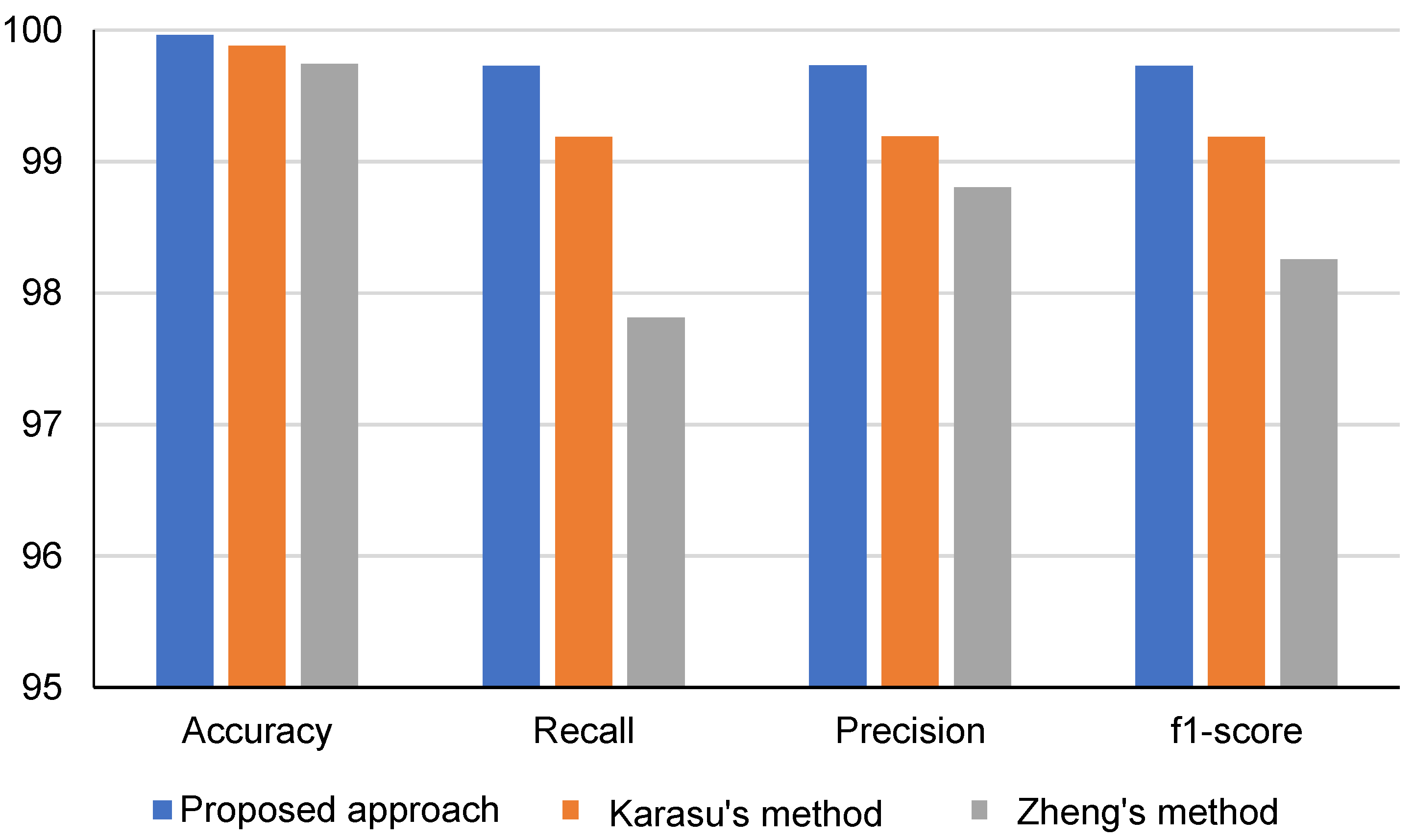
| Index | Karasu’s Method [15,16] | Zheng’s Method [17] | Proposed Approach |
|---|---|---|---|
| Accuracy (%) | 99.88 | 99.74 | 99.97 |
| Precision (%) | 99.19 | 98.80 | 99.81 |
| Recall (%) | 99.18 | 97.81 | 99.80 |
| F1-score (%) | 99.18 | 98.30 | 99.80 |
| Training time per epoch (seconds) | 15 | 16 | 28 |
| Building Size | four 20-foot containers | |
| Load Demand | 10 kWh/day | |
| Solar Generation | The total power generation per day is 7.4 kW × 3.9 h = 28.86 kWh 3.9 h is the average sunshine hours at National Central University, Taiwan | |
| Storage System | Lithium-ion Battery | 21.6 kWh |
| Fuel Cell | 5 kW | |
| Power Inverter | Three-phase 15 kW, AC output voltage is 220 V | |
| PQD | TM | FA | BPNN | WEFNNBT | Karasu’s Method | Zheng’s Method | Proposed Approach |
|---|---|---|---|---|---|---|---|
| Normal | 97.51% | 98.15% | 67.81% | 99.26% | 99.92% | 99.75% | 99.98% |
| Sag | 97.12% | 16.18% | 97.85% | 98.83% | 99.45% | 98.97% | 99.79% |
| Swell | 96.84% | 17.57% | 97.61% | 98.66% | 99.69% | 99.48% | 99.93% |
| Harmonic | 13.72% | 96.42% | 97.15% | 99.17% | 99.91% | 99.81% | 99.97% |
| Transient | 86.34% | 95.83% | 96.92% | 98.22% | 99.88% | 99.76% | 99.97% |
| Flicker | 83.62% | 94.45% | 96.83% | 97.84% | 99.74% | 99.68% | 99.96% |
| Interruption | 12.86% | 15.29% | 97.72% | 98.93% | 99.51% | 99.13% | 99.86% |
Publisher’s Note: MDPI stays neutral with regard to jurisdictional claims in published maps and institutional affiliations. |
© 2022 by the authors. Licensee MDPI, Basel, Switzerland. This article is an open access article distributed under the terms and conditions of the Creative Commons Attribution (CC BY) license (https://creativecommons.org/licenses/by/4.0/).
Share and Cite
Chen, C.-I.; Berutu, S.S.; Chen, Y.-C.; Yang, H.-C.; Chen, C.-H. Regulated Two-Dimensional Deep Convolutional Neural Network-Based Power Quality Classifier for Microgrid. Energies 2022, 15, 2532. https://doi.org/10.3390/en15072532
Chen C-I, Berutu SS, Chen Y-C, Yang H-C, Chen C-H. Regulated Two-Dimensional Deep Convolutional Neural Network-Based Power Quality Classifier for Microgrid. Energies. 2022; 15(7):2532. https://doi.org/10.3390/en15072532
Chicago/Turabian StyleChen, Cheng-I, Sunneng Sandino Berutu, Yeong-Chin Chen, Hao-Cheng Yang, and Chung-Hsien Chen. 2022. "Regulated Two-Dimensional Deep Convolutional Neural Network-Based Power Quality Classifier for Microgrid" Energies 15, no. 7: 2532. https://doi.org/10.3390/en15072532