Simultaneous Distribution Network Reconfiguration and Optimal Allocation of Renewable-Based Distributed Generators and Shunt Capacitors under Uncertain Conditions

Abstract

Smart grid technology has received ample attention in past years to develop the traditional power distribution network and to enable the integration of distributed generation units (DGs) to satisfy increasing demand loads and to improve network performance. In addition to DGs, integration of shunt capacitors (SCs) along with network reconfiguration can also play an important role in improving network performance. Besides, network reconfiguration can help to increase the distributed generation hosting capacity of the network. Some of the research in the literature have presented and discussed the problem of optimal integration of renewable DGs and SCs along with optimal network reconfiguration, while the network load variability and/or the intermittent nature of renewable DGs are neglected. For the work presented in this paper, the SHADE optimization algorithm along with the SOE reconfiguration method have been employed for solving the aforementioned optimization problem with consideration of uncertainty related to both the network load and the output power of the renewable DGs. Maximizing the hosting capacity (HC) of the DGs and reducing network power losses in addition to improving the voltage profile have been considered as optimization objectives. Five different case studies have been conducted considering 33-bus and 59-bus distribution networks. The obtained results validate the effectiveness and the superiority of the employed techniques for maximizing the HC up to 17% and reducing power losses up to 95%. Besides, the results also depict the effect of SC integration and the consideration of uncertainties on achieving the optimization objectives with realistic modeling of the optimization problem.

1. Introduction

Electrical power has been provided efficiently via the electrical power systems for many long years, from large and centralized electricity generating stations to different consumers in homes and in industries. The traditional pattern of power generation and transmission has been changed by the constantly increasing global population and electrical demand loads which have led to saturation of the electric power network, negative environmental impacts from large centralized power generating plants such as global warming and intensive carbon emissions, changes in consumer behavior, and newly emerging techniques to get energy from renewable sources. The traditional electric power network has been developed to be a more intelligent, so-called smart grid technology (SGT) [1].

A smart grid is simply an intelligent electric power network with two ways of power flow and communications, which provide electric systems with better robustness, security, flexibility, reliability, and efficiency. The ability to incorporate one or more small power generators, called distributed generators (DGs), into a distribution network’s feeders is considered one of the main benefits of smart grid technology. A distributed generator (DG) is simply known as an electric power source that is added to distribution network buses or feeders and it is allocated close to different consumers or points of consumption in order to improve network performance and the quality of the delivered power, enhance system reliability, reduce network power losses, and retard the need for new additional costs for the addition of new distribution feeders. There is only one unidirectional way for power flow from the power generating stations to distribution systems in conventional electric power systems. Recently, with the integration of DGs in distribution networks, generated power can flow from distribution feeders to substations, providing two ways of power flow (i.e., bidirectional power flow) [2]. Distributed generators can be employed as prime, standby electric power sources, or even reactive power sources, incorporated in residential, industrial, or commercial areas. From a technological aspect, DGs might be renewable power sources, such as photovoltaic systems, wind turbines, and biomass, or non-renewable conventional sources, such as fuel cells, natural gas, and micro-turbines. Renewable energy sources (RESs) produce output power that is uncertain, very hard to predict with high accuracy, and intermittent as it depends on environmental factors, such as wind speed and solar irradiance. In the past few years, and it is predicted to increase in the near future, RESs are spreading throughout the world, and they have a major contribution to existing power systems. As a result, RESs, with their intermittent nature, are replacing conventional non-renewable sources, which leads to decreasing the power flow predictability in the network. The location and the size of DGs in a distribution network might lead to positive or negative impacts on network performance. Hence, they have to be incorporated into the network after comprehensive planning and study to determine their optimal locations and sizes in order to avert any negative impact, such as overvoltage, exceeding the acceptable loading limits of network feeders, harmonic overloading, etc.

In addition to DGs, installing shunt capacitors (SCs) in distribution systems can improve the power quality and the power factor, enhance the voltage profile, and reduce power losses by injecting reactive power. A shunt capacitor draws a leading current that modifies the characteristics of an inductive load by opposing some or all of the lagging components of the inductive load current at the installation point. Similar to DGs, adding shunt capacitors to distribution systems will be useful only when optimal locations and sizes are applied, and any inappropriate location or size may lead to negative impacts, such as increasing the power losses and/or decreasing the voltage value below the acceptable limit.

In the last few years, several different techniques have been presented in many studies for determining the optimal placement and sizing of DGs or SCs separately in distribution systems. Other researchers have proposed other techniques for simultaneous optimal integration of both DGs and SCs for compensating the real and the reactive power. In [3], different types of DGs, their various technologies, the economic and the technical advantages gained from incorporating DGs in electric power distribution systems and the imposed constraints were presented. The authors in [4,5] presented a comprehensive general view of distributed generation and the evolutions in DG technologies in addition to a review of the different optimization techniques employed for solving the problem of the optimal allocation and sizing of DGs. A novel multi-objective optimization strategy based on the PSO algorithm was presented in [6] for solving the problem of distribution system planning with optimal DG integration. In [7], the authors employed a simple heuristic optimization approach, which was based on loss sensitivity analysis for solving the problem of optimal DG allocation in distribution networks with the objective of minimizing network power losses. The problem of optimal allocation of DGs in distribution networks was handled in [8] using the GA optimization algorithm and considering economic and technical objectives. In [9], an advanced variant of the PSO algorithm was employed to solve the problem of optimal DG allocation, considering the objectives of maximizing annual savings and enhancing the bus voltage and feeder current profiles. The Kalman filter algorithm was employed in [10] for finding the optimal allocation of DGs in the distribution system. The authors in [11] employed a strategy, which was based on a voltage stability index and used the combined sensitivity factor analogy for solving the problem of the optimal allocation and sizing of DGs with multiple types in a 48-node distribution network, considering the objectives of reducing network power losses and enhancing the bus voltage profile. The genetic algorithm was been used in [12] for solving the optimal allocation problem of DGs in the distribution system for minimizing power losses. In [13], the problem of optimal DG sizing was handled and solved by achieving the objectives of minimizing the costs of DGs and maximizing network loadability. The authors in [14] employed the GA and the optimal power flow solution for solving the problem of simultaneous optimal allocation of both shunt capacitors and voltage regulators with achieving optimal investment costs. The fuzzy GA was employed in [15] for solving the problem of optimal allocation of shunt capacitors in distribution systems with the objective of power factor improvement. In [16], the mixed-integer nonlinear programming technique (MINLP) was employed to solve the problem of optimal placement and sizing of shunt capacitors in distribution systems. An optimization approach was presented and employed in [17] for solving the problem of optimal placement and sizing of shunt capacitors and active power conditioners in distribution systems for power quality improvement. To improve the performance of the power system, the grey wolf optimization technique was employed in [18] for determining the optimal sizing of reactive power. Optimal simultaneous placement of both DGs and shunt capacitors in the distribution system was presented in [19,20,21,22] for reducing or minimizing system power losses. In [23], a pareto multi-objective PSO technique was employed for determining the optimal placement and sizing of DGs and shunt capacitors in a distribution network with consideration of network load-related uncertainty, which was modeled using fuzzy logic. Enhanced meta-heuristic optimization methods were employed in [24] for solving the problem of optimal simultaneous allocation of DGs and shunt capacitors in distribution systems, considering demand load variability and with the objectives of minimizing annual power losses and bus voltage profile improvement. The authors in [25] employed the binary collective animal behavior optimization technique for optimal simultaneous placement and sizing of DGs and shunt capacitors in distribution systems for achieving the objectives of minimizing power losses and improving the voltage profile. In [26], the biogeography-based optimization technique was employed to solve the problem of DGs and shunt capacitors optimal allocation with consideration of the optimization objectives of minimizing the total harmonic distortion, minimizing power losses, and improving the voltage profile. The intersect mutation differential evolution (IMDE) optimization technique was presented in [27] for simultaneous optimal allocation and sizing of DGs and shunt capacitors, with the objective of minimizing the power losses and subject to satisfying the bus voltage and feeder current constraints. In [28], GA optimization strategy was employed for optimal simultaneous sizing of both DGs and shunt capacitors, with the objective of minimizing investment and maintenance costs. The authors in [29] presented and employed a sorting-based, non-dominant, multi-objective PSO optimization algorithm, with consideration of fuzzy decision principles for simultaneous optimal placement of renewable DGs and shunt capacitors. Different optimization techniques were employed in [30,31,32] for optimal allocation and sizing of DGs and shunt capacitors in distribution systems, with the consideration of minimizing power losses as the optimization objective. Optimal allocation of shunt capacitors in a distribution system integrated with wind energy-based DGs was performed in [33] by using a stochastic technique, which was based on a point estimation method. A hybrid optimization approach of weight improved PSO and the gravitational search algorithm (GSA) was employed in [34] for optimal DG and shunt capacitor allocation and sizing. In [35], simultaneous optimal placement of DGs and shunt capacitors was performed with consideration of the intermittency and uncertainty associated with DGs.

In addition to installing shunt capacitors (SCs) and distributed generation units (DGs), distribution network power loss reduction can also be achieved by reconfiguring the existing network topology. A distribution network includes two types of switches, namely sectionalizing and tie-switches. Although both types of switches are principally the same, tie switches are those switches in the network that remain open (normally opened) to preserve the radial structure of the network, while sectionalizing switches are those switches that remain closed (normally closed). To provide appropriate voltage control and protection coordination, radial topology is mostly recommended, and it is preferred for distribution systems. Each node in the radial distribution network has only one way to the substation node, and no loops exist in the network. Distribution network reconfiguration (DNR) can be simply defined as the process of changing the existing network topology or configuration via altering the opened/closed status of tie and sectionalizing switches, such that the radial structure of the network is preserved, all of the network loads are connected, all objectives are achieved, and all considered constraints are satisfied. The main and the conventional objective of network reconfiguration is power loss reduction and alleviating the overload of network feeders. However, distribution network reconfiguration has been employed in the literature for achieving other objectives, such as improving power quality and network loadability, enhancing the voltage profile, reducing operational costs and emissions, and providing more reliable and economic network operation [36,37,38,39,40,41,42,43,44,45,46,47]. Moreover, DNR has been performed for unbalanced distribution networks [48,49], managing distribution system outages [50], reducing annual energy losses [51], estimation of active distribution system states [52], an active distribution network with electric vehicles [53], an active distribution network with DGs [54], etc. On the other hand, other research related to DNR has provided more efficient and effective computations via parallel computation on graphics processing units [55], an extended fast decoupled Newton–Raphson power flow methodology [56], an accelerating decomposition technique [57,58], and fast calculations for involved frequent power flow solutions [54]. In addition, distribution network reconfiguration has also been employed in the literature as an approach for maximizing the distributed generation hosting capacity (i.e., the DG penetration that can be accommodated) of the network [59,60].

The limited electric power generation and variability associated with distribution system demand loads make the process of operating and controlling a distribution system a difficult and a complicated task, especially with high load densities. Minimized system power losses cannot be achieved considering the same network configuration for all levels of variable system loads, consequently, frequent reconfiguration of the network is required; and, for satisfying the required demand loads, DGs and SCs are incorporated in the network and this leads to a decrease in power losses, an enhanced voltage profile, alleviation of the feeders’ overload, and improved reliability and efficiency of the power supply. For solving the problem of distribution network reconfiguration and DG and SC optimal integration, the variability associated with the network demand load in addition to the intermittent output power from renewable DGs must be considered. Allocation and sizing of integrated DGs and SCs in the distribution network, which is determined using voltage or loss indices, may not be the optimal solution for all network configurations; hence, distribution network reconfiguration and shunt capacitor and distributed generator integration need to be performed simultaneously to provide an optimal solution for minimizing power losses and enhancing network operation and the voltage profile.

Several different types of research in the literature have focused on the static single-hour DNR for providing an appropriate and fixed network configuration for a certain time duration—which can be an hour, a year, a season, or as required and applicable—without considering either the variations of DG unit output power with time or the variable network demand load where both of the generated power and demand loads are set to their peak or average values [61,62,63]. Accordingly, the static single-hour DNR will not lead to an optimal solution for the DNR problem for distribution networks integrated with renewable DG units with intermittent output power, such as PV units or wind turbines. In light of the above, other research in the literature investigated the dynamic multi-hour DNR to account for the intermittent nature of renewable DGs and the variability associated with the network demand loads [64,65]. Using dynamic DNR, the optimal configurations for multiple networks are provided for different hours or durations based on the variations of loads and the power generation of DGs with achieving the optimization objective, mainly the minimization of network power losses and satisfying the considered constraints for all provided configurations. In conclusion, the static DNR is more economically beneficial than dynamic reconfiguration, where a fixed configuration is provided and the cost of more switching actions is avoided. However, optimal and more accurate solutions are provided using the dynamic approach for the networks integrated with renewable DGs with intermittent output power.

Considering variable demand loads, distribution network reconfiguration problems were presented in [66,67]. Seasonal distribution network reconfiguration was presented in [68], and the related switches to be opened or closed for changing the network configuration were determined. Although the variability of demand loads has been considered in [66,67,68] for distribution network reconfiguration, the output power of DG units has been considered a constant value disregarding the associated variability. In [69,70], optimal network configurations for the day ahead have been provided by applying multi-hour dynamic reconfiguration based on foreseen values for the power generation and demand loads. Multi-hour DNR has been performed in [71] with consideration of variable demand loads and renewable DGs with the objective of power loss minimization. Distribution network reconfiguration was performed in [72] to provide the optimal seasonal network configuration, considering variable demand load and renewable DG output power. In [73,74,75], the effect of considering the load variability and the uncertainty associated with renewable DG output power on the reconfiguration process of the distribution network was studied. Distribution network reconfiguration with the integration of distributed generators was performed in [76] as a mixed-integer linear programming problem. Optimal DG allocation and distribution network reconfiguration using a heuristic algorithm based on sensitivity indices for power loss minimization was presented in [77]. The problem of distribution network reconfiguration along with distributed generation allocation was modeled in [78] as a multi-objective nonlinear mixed-integer programming problem, with a consideration of the demand load variability and the uncertainties associated with the output power of renewable DGs. Simultaneous optimal network reconfiguration and DG allocation in distribution networks was presented in [79] using a meta-heuristic harmony search algorithm (HAS), while the same problem was presented in [80], using an adaptive genetic algorithm and a graph theory. In [81], distribution network reconfiguration with distributed generation integration was presented for network reliability improvement and power loss minimization. A simulated annealing technique was used in [82] for distribution network feeder reconfiguration and capacitor setting to reduce power loss and to improve the voltage profile. In [83], a mixed-integer non-linear programming technique was used for optimal distribution network reconfiguration and shunt capacitors allocation with the objective of power loss minimization, while the same problem was presented in [84], using the ant colony search optimization technique. Simultaneous optimal network reconfiguration and shunt capacitor allocation in a distribution network was presented in the literature using a genetic algorithm [85], a modified particle swarm optimization algorithm [86], a hybrid optimization technique using a minimal nodal voltage approach and a genetic algorithm [87], the Chu–Beasley based genetic algorithm [88], a fuzzy-genetic algorithm [89], ordinal optimization [90], a minimum spanning tree algorithm [91], and a selective particle swarm optimization [92] and harmony search algorithm [93].

In view of the above and according to the authors’ best knowledge, simultaneous distribution network reconfiguration with optimal allocation and sizing of renewable distributed generators and shunt capacitors for minimizing network power loss, maximizing the DG hosting capacity, and improving the voltage profile, as optimization objectives, with consideration of the network demand load variability and the uncertain parameters related to the considered renewable DGs, haven’t been presented so far. Hence, for the work presented in this paper, the optimal allocation and sizing of renewable DGs (PV units and wind turbines) and shunt capacitors in the distribution network are implemented simultaneously with the network reconfiguration, such that network power losses are minimized, distributed generation hosting capacity of the network is maximized, and the voltage profile is enhanced, while keeping the considered constraints within their desired and acceptable limits. The 33-bus distribution network and 59-bus real distribution network in Cairo, Egypt, are considered for this study, taking into consideration the variability of demand loads in addition to the uncertainty associated with the output power from the considered renewable DGs in the optimization problem using the scenario-based technique. As indicated before, the output power from renewable DGs depends on environmental factors (such as wind speed and solar irradiance), which have an intermittent nature, and they are very difficult to predict. The uncertainty in the demand load is modeled using the normal probability density function (PDF), while the stochastic wind speed is modeled using Weibull PDF, and the stochastic solar irradiance is modeled using lognormal PDF. For each of these uncertain parameters, one thousand scenarios are generated by running a Monte Carlo simulation, and then a scenario reduction technique called the backwards scenario reduction technique is applied to select a specific number from the generated scenarios. The optimization process shall be performed by using the success history-based adaptive differential evolution algorithm (SHADE) [94], which is an advanced variant of the differential evolution algorithm (DE). In the literature, there are three different categories for the reconfiguration techniques, namely, evolutionary algorithms (EAs) [61,62,95,96], mathematical programming (MP) [63,65,76,97,98], and heuristics-based techniques [99,100]. For the work presented in this paper, the heuristics-based reconfiguration method presented in [101], called the switch opening and exchange method (SOE), will be adopted for distribution network reconfiguration. This method will be illustrated in detail within Section 4, using a three-feeder small example system.

The rest of the paper will be organized as follows: the adopted model for the variability and the uncertainty associated with demand load, wind speed, and solar irradiance is described in Section 2. The problem formulation with the definition of variables, optimization objectives, and considered constraints is given in Section 3. The employed reconfiguration method (SOE method) is illustrated in Section 4. An overview of the success history based adaptive differential evolution optimization algorithm (SHADE) is outlined in Section 5. The simulation results analysis and the discussion are given in Section 6. Final conclusions and recommendations for future work are listed in Section 7.

2. Modeling of Load Demand Variability, Stochastic Wind Speed, and Solar Irradiance

This section discusses and explains modeling of the uncertainty associated with demand load, wind speed, and solar irradiance via scenario generation and reduction techniques.

The variability of load demand is modeled using the normal probability density function (PDF) with an associated mean (μ_d) and standard deviation (σ_d). The probability density of uncertain demand load (P_d) is expressed as follows:

$${\Delta }_d\left(P_d\right)= \frac{1}{{\sigma }_d\sqrt{2\pi }}exp\lfloor -\frac{{\left(P_d-{\mu }_d\right)}^2}{2{\sigma }_d^2}\rfloor$$

(1)

Based on this normal distribution of demand load, one thousand scenarios are generated using a Monte Carlo simulation.

The uncertainty associated with wind speed, which affects the output power from wind turbines, is modelled using the Weibull PDF, which is usually used for representing wind speed distribution. The probability density of uncertain wind speed (ν_w) is expressed as follows:

$${\Delta }_{\nu }\left({\nu }_w\right)=\left( \frac{\beta }{\alpha }\right) {\left(\frac{{\nu }_w}{\alpha }\right)}^{\left(\beta -1\right)} exp\lfloor -{\left(\frac{{\nu }_w}{\alpha }\right)}^{\beta }\rfloor for 0<{\nu }_w<\infty$$

(2)

where $\alpha$ is the scale parameter and $\beta$ is the shape parameter for the Weibull PDF. Based on this distribution of wind speed, one thousand scenarios are generated using a Monte Carlo simulation.

The uncertainty associated with solar irradiance, which affects the output power from PV units, is modelled using the lognormal PDF, with mean $\left({\mu }_s\right)$ and standard deviation $\left({\sigma }_s\right)$, which is usually used for representing solar irradiance distribution. The probability density of uncertain solar irradiance $\left(G_s\right)$ is expressed as follows:

$${\Delta }_G\left(G_s\right)=\frac{1}{G_s{\sigma }_s\sqrt{2\pi }}exp \lfloor \frac{-{\left(\mathit{ln}{G}_s-{\mu }_s\right)}^2}{2{\sigma }_s^2}\rfloor for G_s>0$$

(3)

Similar to demand load and wind speed, based on the lognormal distribution, one thousand scenarios are also generated using a Monte Carlo simulation. These generated scenarios for solar irradiance consider that sunlight is not available during the whole day and usually it is available only half of the day. Hence, the solar irradiance and, accordingly, the output power from PV units is zero during this period of the day.

The scenario generation technique followed in the work presented in this paper shall be the same technique presented in [102], where the generated one thousand scenarios, as discussed above, for demand load, wind speed and solar irradiance are combined, which results in one thousand scenarios with each scenario including three values (demand load, wind speed, and solar irradiance); hence, the i^th scenario (S_i) can be represented as S_i = [P_d,i, ${\nu }_{w,i}$, G_s,i].

As it is impractical to handle so many scenarios, an appropriate scenario reduction technique is necessary. In this paper, the scenario reduction technique presented in [102]—called the backward reduction technique—shall be applied in order to reduce the generated one thousand scenarios to thirty scenarios only, which is practically a good number of scenarios for optimization problems. In this technique, the procedure of scenario reduction depends on the distance between each pair of scenarios, where one scenario (the scenario with lower probability) is removed from the pair of scenarios having minimum distance and this procedure is repeated until the required number of scenarios is reached. The thirty scenarios resulting from the applied scenario reduction technique with their respective probabilities are listed below in

Table 1. Resulting scenarios from the applied scenario reduction technique (30 Scenarios).

Scenario No.	Load Level (%)	Wind Speed (m/s)	Solar Irradiance (W/m2)	$\mathbf{Scenario} \mathbf{Probability} ({\mathit{p}}_{\mathit{s}})$
1	33.09869	0	0	0.02363
2	33.82429	8.1	0	0.02432
3	34.79878	4.6	0	0.03139
4	34.85638	11.5	0	0.02454
5	42.43202	3.5	0	0.04030
6	43.78283	10.4	0	0.05023
7	44.43556	5.8	448	0.01507
8	45.37022	8.1	0	0.09349
9	46.58196	9.2	900	0.04692
10	46.80610	12.7	0	0.03744
11	47.00383	0	0	0.04441
12	47.66340	13.8	520	0.02420
13	48.58249	16.1	0	0.02877
14	49.39537	3.5	0	0.06975
15	49.46533	13.8	814	0.04384
16	54.70679	6.9	0	0.03664
17	54.97036	0	0	0.03916
18	55.89388	11.5	455	0.02603
19	55.97981	0	263	0.02180
20	58.78500	10.4	856	0.01712
21	59.61178	4.6	529	0.02957
22	60.01654	11.5	1	0.02546
23	65.52149	4.6	842	0.01507
24	69.68230	4.6	0	0.02386
25	70.07522	9.2	0	0.03219
26	72.52334	0	0	0.01393
27	76.89657	10.4	935	0.03984
28	78.68899	6.9	0	0.05479
29	86.35351	13.8	363	0.01062
30	93.01955	10.4	478	0.01564

. As mentioned before, each scenario represents values for demand load (as a percentage of total load), wind speed, and solar irradiance. Based on the values of wind speed and solar irradiance, wind and solar power (output power from wind turbines and PV units) are calculated as discussed in the following paragraphs.

For a wind turbine with rated power $P_{rated}^{WT}$, the output power generated as a function of wind speed $\left({\nu }_w\right)$ can be calculated as follows:

$$P^{WT}\left(v_w\right)=\{\begin{array}{ll}0\hfill & for v_w<v_{cut\text{-}in} and v_w>v_{cut\text{-}out}\hfill \\ P_{rated}^{WT}\left(\frac{v_w-v_{cut\text{-}in}}{v_{w,rated}-v_{cut\text{-}in}}\right)\hfill & for v_{cut\text{-}in}\le v_w\le v_{w,rated}\hfill \\ P_{rated}^{WT}\hfill & for v_{w,rated}\le v_w\le v_{cut\text{-}out}\hfill \end{array}$$

(4)

where $v_{cut\text{-}in}$, $v_{cut\text{-}out}$ and $v_{w,rated}$ are the cut-in, cut-out, and rated wind speed of the turbine, respectively.

For a PV unit with rated power $P_{rated}^{PV}$, the output power generated as a function of solar irradiance $\left(G_s\right)$ can be calculated as follows:

$$P^{PV}\left(G_s\right)=\{\begin{array}{ll}{P}_{rated}^{PV}\left(\frac{G_s^2}{G_{std} R_c}\right)\hfill & for 0<G_s<R_c\hfill \\ P_{rated}^{PV}\left(\frac{G_s}{G_{std}}\right)\hfill & for G_s\ge R_c\hfill \end{array}$$

(5)

where $G_{std}$ and $R_c$ are the standard environment solar irradiance and specified irradiance value, respectively.

3. Problem Formulation

3.1. Objective Function

In this section, a multi-objective optimization problem is formulated for maximizing the distributed generation probabilistic hosting capacity (PHC) of the distribution network, minimizing network power losses (i.e., maximizing the reduced power losses ($R{P}_{loss}$)), and improving the voltage profile, while satisfying the operational constraints and limits for different scenarios of load demand, wind speed, and solar irradiance. The objective function for the optimization problem can be formulated as follows:

$$Maximize PHC(\%)={\displaystyle \sum }_{s=1}^{N^s}H{C}_s.p_s$$

(6)

$$Maximize R{P}_{loss}(\%)=\frac{P_{loss}^0-P_{loss}}{P_{loss}^0}\times 100$$

(7)

where $H{C}_s$ is the hosting capacity of DGs for the s^th scenario, $p_s$ is the probability related to a scenario (s), $N^s$ is the total number of scenarios, $P_{loss}^0$ is the total network power loss at normal loading conditions (Base Configuration), and $P_{loss}$ is the probabilistic total network power loss for all of the studied scenarios. The $H{C}_s$ and the $P_{loss}$ can be calculated as follows:

$$H{C}_s(\%)=100\frac{{{\displaystyle \sum }}_{n_{WT}}{P}_{n_{WT},s}^{WT}+{{\displaystyle \sum }}_{n_{PV}}{P}_{n_{PV},s}^{PV}}{{{\displaystyle \sum }}_{n=1}^{N^{nodes}}{P}_n^L}$$

(8)

$$P_{loss}={\displaystyle \sum }_{s=1}^{N^s}\left({\displaystyle \sum }_{b=1}^{N^{line}}\left({\left|I_{b,s}\right|}^2· r_b\right).p_s\right)$$

(9)

where $P_{n_{WT},s}^{WT}$ is the output power of the wind turbine allocated at the bus or the node ($n_{WT})$ for scenario (s), $P_{n_{PV},s}^{PV}$ is the output power of the PV unit allocated at the bus or the node ($n_{PV})$ for scenario (s), $P_n^L$ is the load power at the $n^{th}$ node, $N^{nodes}$ is the total number of network nodes, $\left|I_{b,s}\right|$ is the magnitude of the current flowing in the $b^{th}$ branch for scenario (s), $r_b$ is the $b^{th}$ branch resistance, and $N^{line}$ is the total number of network lines or branches.

For improving the voltage profile, minimizing the overall aggregated voltage deviation index ($AVD{I}_{ov})$ for all different considered scenarios is also set as an objective for the optimization problem. For each scenario, the aggregated voltage deviation index ($AVD{I}_s)$ is calculated as the sum of voltage deviations of load buses from unity as follows:

$$AVD{I}_s={\displaystyle \sum }_{lb=1}^{N^{lb}}1-V_{lb,s}$$

(10)

where $V_{lb,s}$ is the voltage at the load bus ($lb$) for scenario (s), and $N^{lb}$ is the total number of load buses. Hence, the objective for minimizing the overall aggregated voltage deviation index ($AVD{I}_{ov})$, for all considered scenarios, can be formulated as follows to ensure that voltages at the network load buses are close to unity:

$$Minimize AVD{I}_{ov}={\displaystyle \sum }_{s=1}^{N^s}AVD{I}_s.p_s$$

(11)

3.2. Optimization Constraints

The operational and planning constraints applied for the considered optimization problem shall be as follows:

$$P_{n_{WT},rated}^{WT}\le P_{max}^{WT}$$

(12)

$$P_{n_{PV},rated}^{PV}\le P_{max}^{PV}$$

(13)

$$H{C}_s\le 100$$

(14)

$$\left|I_{b,s}\right|\le I^{rated}$$

(15)

$$V^{min}\le \left|V_{n,s}\right|\le V^{max}$$

(16)

where $P_{n_{WT},rated}^{WT}$ and $P_{n_{PV},rated}^{PV}$ are the rated output power or capacity of the wind turbine and the PV unit allocated at nodes $n_{WT}$ and $n_{PV}$, respectively. The $P_{max}^{WT}$ and the $P_{max }^{PV}$ are the maximum allowed rated power or capacity for the wind turbine and the PV unit, respectively. The $I^{rated}$ is the maximum allowed current of a network branch, $\left|V_{n,s}\right|$ is the magnitude of voltage at the $n^{th}$ node, $V^{min}$ and $V^{max}$ are the minimum and the maximum allowed node or bus voltage, respectively.

4. Switch Opening and Exchange Method

The switch opening and exchange method (SOE) employed in this paper for performing the distribution network reconfiguration is a novel heuristic method which was first proposed in [101] for efficient solving of large-scale multi-hour stochastic distribution network reconfiguration and it has proven its superiority to other heuristic algorithms, EAs, and MPs in terms of accuracy and/or solution speed. This method includes three stages and it adopts both of the sequential switch opening and branch exchanging techniques for solving the reconfiguration problem, where the first stage applies the sequential switch opening, while the second and the third apply the branch exchanging. These stages shall be illustrated in detail within the following paragraphs, using the three-feeder distribution system shown below in Figure 1 as an example system.

4.1. Stage 1: Sequential Switch Opening

The status of all switches in this stage is initially set to be closed which forms loops in the distribution network. In each iteration, the status of only one switch (selected from the sectionalizing closed switches within the loops) is changed to be opened (i.e., changed to be a tie-switch) and the loop, where that switch is located, is opened. Hence, the number of iterations in this stage shall be equal to the number of loops in the network and the above procedure is repeated in each iteration till all loops are opened and the network becomes radial. The criteria for selecting the sectionalizing switch to be opened or changed to a tie-switch in each iteration shall be as follows:

(a)

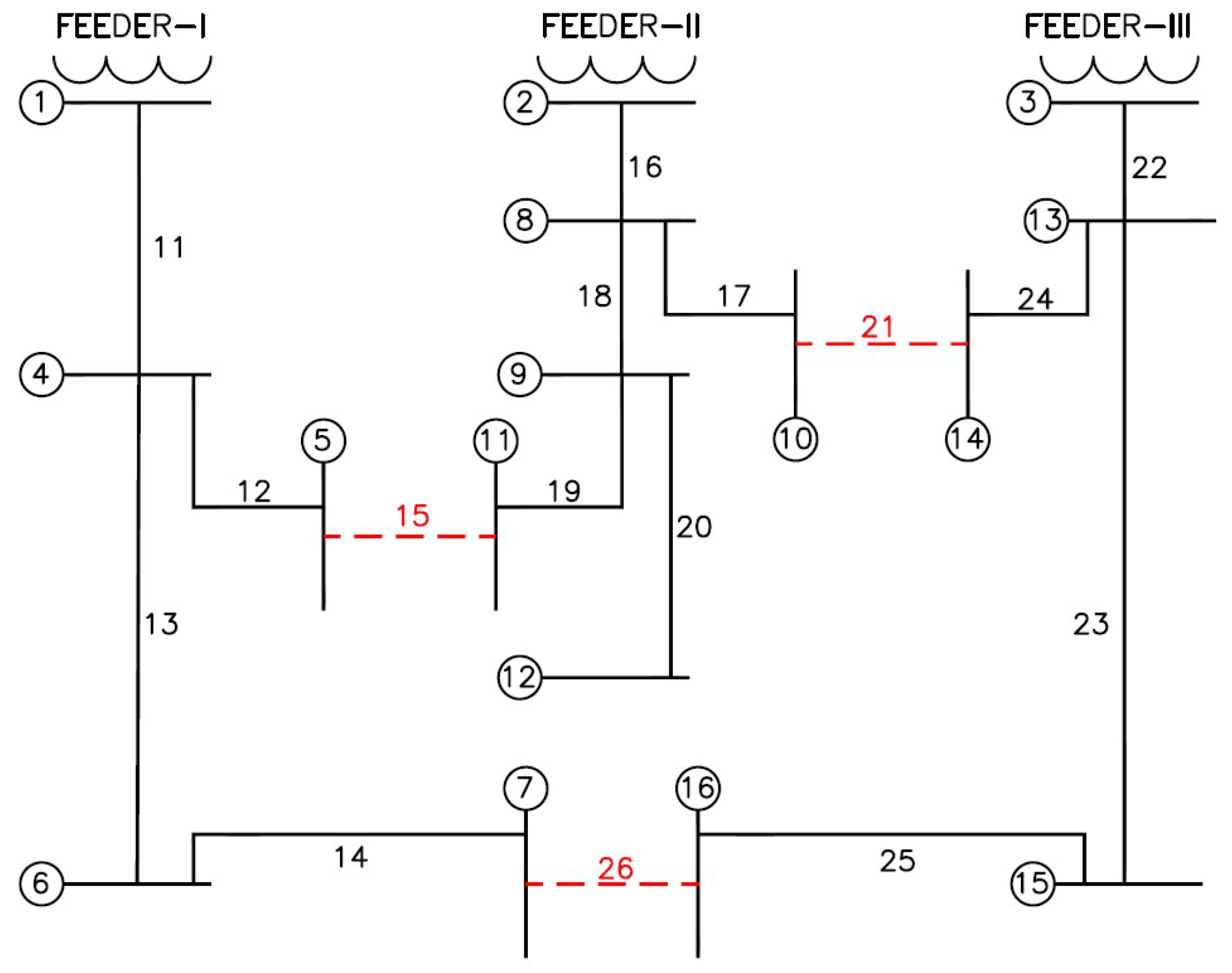
Based on the network configuration, close all of the network switches and determine the sectionalizing switches or branches within the formed loops. In the above example system, closing all switches forms three loops that include all of the system branches except for branch 20 (connecting nodes 9 and 12), which is not included within any of the formed loops. Hence, three iterations shall be required in thin stage for this system to select which sectionalizing switches to be changed to tie-switches.

(b)

For each switch within the loops:

b.1.

Open the switch.

b.2.

Check the network connectivity (i.e., ensure that there is a path for each node to the substation node).

b.3.

If the network is not connected, assign a large value (e.g., 10⁶) for the network power loss.

b.4.

Else if the network is connected, provide the power loss value for the network after opening the switch.

b.5.

Close the opened switch.

b.6.

The above-described steps (from b.1 to b.5) are repeated for all other remaining sectionalizing switches within the loops.

b.7.

Permanently open the switch that achieves the minimum network power loss value among all other switches. This will consequently open the loop where this switch is located.

b.8.

The above steps (from b.1 to b.7) are repeated for the sectionalizing switches within the remaining loops until the network becomes radial (i.e., all loops are opened). The obtained radial network configuration is called the “initial configuration”.

b.9.

Provide the power loss value associated with the obtained radial network configuration and record this value as “loss-0”.

4.2. Stage 2 & Stage 3: Branch Exchanging

In these stages, other different radial configurations are generated from the initial configuration obtained from the first stage searching for a better solution. This is achieved by opening a sectionalizing switch in the initial configuration (i.e., changing it to a tie-switch) and then applying the steps of the first stage (keeping the status of that switch to be opened) which leads to a different radial network configuration. This procedure is applied to the other sectionalizing switches in the initial configuration to generate other radial configurations. Hence, for all sectionalizing switches within the initial configuration, the following procedure shall be applied:

(a)

Open the sectionalizing switch and apply the steps of the first stage as described above, but keep the status of this switch at permanently opened, which leads to a different radial network configuration.

(b)

Provide and record the power loss value associated with the obtained radial configuration.

(c)

Close the opened switch.

(d)

The above steps (from a to c) are repeated for the other remaining sectionalizing switches in the initial configuration.

In order to avoid the computational complexity, the following sets of sectionalizing switches (in the initial configuration) are excluded from the above procedure:

Set-1. 

This set includes any sectionalizing switch in the initial configuration whose shortest path to the substation node includes n₁ or less sectionalizing switches. If n₁ = 2, then for the above example system this set shall include the sectionalizing switches 1–4, 4–5, 4–6, 2–8, 8–10, 8–9, 3–13, 13–14, and 13–15. The sectionalizing switch (x-y) refers to the switch associated with the branch connecting the nodes x and y.

Set-2. 

This set includes any sectionalizing switch, in the initial configuration, whose shortest path to an ending node includes n₂ or less sectionalizing switches and it is upstream of the same ending node. If node A locates in the shortest path of node B to the substation node, then it can be said that node A is upstream of node B and node B is downstream of node A. The node that has no downstream nodes is referred to as the “ending node”. If n₂ = 1, then for the above example system, this set shall include the sectionalizing switches 4–5, 9–11, 8–10, 13–14, 6–7, and 15–16. In this work, the values assigned for the above-mentioned parameters (n₁ & n₂) shall be 3 & 2, respectively.

Set-3. 

This set includes any sectionalizing switch, in the initial configuration, which is not located in a loop when all of the network switches are closed. For the above example system, this set shall only include the sectionalizing switch 9–12.

(e)

For each radial configuration obtained from the above steps (from a to d), the following procedure shall be applied:

e.1.

Determine the set of sectionalizing switches as defined above in “Set-2”.

e.2.

Exclude the sectionalizing switches as defined above in “Set-1” and “Set-3” from the sectionalizing switches obtained from e.1., and apply the following for each of the remaining switches:

e.3.

Determine the available open-1-close-1 actions which include opening that sectionalizing switch. Open-1-Close-1 action (O1C1) is defined as the action of opening one switch and closing another without affecting either the network connectivity nor the radiality. For the example, in the system in Figure 1, if the switch (6–7) is opened, then there will only be one available action to ensure network connectivity, which is to close the switch (7–16). The following is another example: if the switch (2–8) is opened, then there will be two available actions to ensure network connectivity, which are to close the switch (10–14) or (5–11).

e.4.

Execute the found available O1C1 actions, then provide the associated power loss value after executing each action, and record this value as a new element in a vector named “loss-1”.

e.5.

Determine the O1C1 actions that lead to a decrease in the network power loss value. These O1C1 actions are referred to as “objective decreasing O1C1 actions”.

e.6.

Combine and execute any two independent O1C1 actions in the set of objective decreasing O1C1 actions, then provide the associated power loss value after executing the combined actions and record this value as a new element in a vector named “loss-2”. Two O1C1 actions are called “independent actions” when none of the network feeder(s) involved in one O1C1 action are the same as any of the feeder(s) involved in the other action, the network feeder that includes a branch, directly connected to the substation node, in addition to the downstream branches. For the example system in Figure 1, there are 3 independent feeders which include the branches (1–4), (2–8), and (3–13) in addition to their downstream branches.

e.7.

The above steps (from e.1 to e.6) are repeated for the other radial configurations.

(f)

Find the minimum power loss value recorded in “loss-0”, “loss-1”, and “loss-2“. The corresponding network configuration shall be the optimal solution for the reconfiguration problem.

The pseudo-code of SOE method, provided below in Algorithm 1, can help for a better understanding of the above-described steps:

Algorithm 1: SOE Method
Sequential Switch Opening
1	Close all of the network switches
2	For each switch within a loop do
3	Open the switch
4	if the network is connected then
5	calculated the power losses Ploss
6	else
7	Assign large value for Ploss
8	end
9	Close the switch
10	end
11	Permanently open the switch corresponding to minimum Ploss
12	Repeat above steps (from 2 to 12) till radial configuration is obtained “Initial Configuration”.
13	Calculate Ploss for the obtained initial configuration and store the value as “loss-0”
Branch Exchanging
14	For each sectionalizing switch in the initial configuration (excluding those included in set-1, set-2 and set-3) do
15	Permanently open the switch
16	Keeping that switch opened, apply above steps (from 1 to 13)
17	Calculate Ploss for the obtained radial configuration and store the obtained value
18	Close the opened switch
19	end
20	For each radial configuration obtained after applying above steps (from 14 to 16) do
21	Determine “set-2” sectionalizing switches and exclude any switch related to “set-1” or “set-3”
22	For each switch obtained from previous step do
23	Determine the available open-1 close-1 (O1C1) actions
24	Execute each O1C1 action, calculate the related Ploss and store the obtained value in a vector “loss-1”
25	Determine the objective decreasing O1C1 actions
26	Combine and execute any two independent objective decreasing actions, calculate the related Ploss and store the obtained value in a vector “loss-2”
27	end
28	end
29	The configuration corresponding to minimum power loss value stored in “loss-0”, “loss-1” and “loss-2” is con-sidered as the optimal network con-figuration.

5. Success History Based Adaptive Differential Evolution Algorithm (SHADE)

The SHADE algorithm is an advanced variant of the differential evolution optimization algorithm, which is employed for solving the optimization problem presented in this paper. Differential Evolution (DE) is a population-based stochastic optimization algorithm, which initializes with randomly generated individuals that evolve via probabilistic operators, such as mutation and recombination. The performance of the DE algorithm depends mainly on the population size$\left(N_p\right)$, mutation and/or crossover strategies, the scale factor (F) associated with mutation, and the crossover rate (CR) associated with recombination. In order to do away with the tuning of parameters, adaptive mechanisms for online adjustment of the control parameters during the evolution have been investigated and a history based parameter adaptation scheme has been proposed (SHADE). The SHADE algorithm is discussed in detail within the following subsections, which starts with initialization, and then it is followed by an iterative procedure including mutation, crossover, and selection.

5.1. Initialization

The population of candidate solutions with randomly assigned values is created during the initialization. To ensure that the randomly generated values are within the defined upper and lower bounds, the j-th component of the i-th decision vector is generated as follows:

$$x_{i,j}^{\left(1\right)}= x_{min,j}+ ran{d}_{i,j} \left[0,1\right] \left(x_{max,j}-x_{min,j}\right)$$

(17)

where $ran{d}_{i,j} \left[0,1\right]$ is a uniform random number between 0 and 1 and the superscript (1) represents initialization. For a population size ($N_p)$ and dimensions of a candidate solution ($d)$, $i=1,2,3,\dots \dots \dots ,N_p$ and $j=1,2,3,\dots \dots \dots ,d$.

5.2. Mutation

For a given generation (t), mutation operator generates a mutant vector $v_i^{\left(t\right)}$ corresponding to each population member $x_i^{\left(t\right)}$ as follows:

$$v_i^{\left(t\right)}= x_i^{\left(t\right)}+ F_i^{\left(t\right)}.\left(x_{pbest}^{\left(t\right)}-x_i^{\left(t\right)}\right)+F_i^{\left(t\right)}\left(x_{r_1^i}^{\left(t\right)}-x_{r_2^i}^{\left(t\right)}\right)$$

(18)

where $r_1^i$ and $r_2^i$ are mutually exclusive integers randomly chosen from the population range, $x_{pbest}^{\left(t\right)}$ is randomly selected from best individuals of current generation, and $F_i^{\left(t\right)}$ is a positive scale factor at t^th generation.

After performing the mutation, if an element $v_{i,j}^{\left(t\right)}$ violates the search boundaries [$x_{min,j},x_{max,j}]$, it is corrected as follows:

$$v_{i,j}^{\left(t\right)}=\{\begin{array}{cc}(x_{min,j}+x_{i,j}^{\left(t\right)})/2& if{v}_{i,j}^{\left(t\right)}<x_{min,j}\\ (x_{max,j}+x_{i,j}^{\left(t\right)})/2& if{v}_{i,j}^{\left(t\right)}>x_{max,j}\end{array}$$

(19)

5.3. Parameter Adaptation

For a generation (t), each included individual has a scale factor $F_i^{\left(t\right)}$ and a crossover rate $C{R}_i^{\left(t\right)}$ which are used to provide a new population of solutions. These parameters are updated as follows:

$$F_i^{\left(t\right)}=randc \left(\mathsf{\mu }{F}_{r_i}^{\left(t\right)}, 0.1\right)$$

(20)

$$C{R}_i^{\left(t\right)}= randn \left(\mathsf{\mu }C{R}_{r_i}^{\left(t\right)}, 0.1\right)$$

(21)

where $randc \left(\mathsf{\mu }{F}_{r_i}^{\left(t\right)}, 0.1\right)$ provides a value through the Cauchy distribution with location parameter $\mathsf{\mu }{F}_{r_i}^{\left(t\right)}$, randomly chosen from a set of successful scale factors of previous generations stored in a memory M of size H, and the scale parameter 0.1, $randn \left(\mathsf{\mu }C{R}_{r_i}^{\left(t\right)}, 0.1\right)$ is a value sampled from a normal distribution with the mean $\mathsf{\mu }C{R}_{r_i}^{\left(t\right)}$, one of the means of successful crossover rates from previous generations stored in the memory M, and 0.1 variance. All $\mathsf{\mu }F$ and $\mathsf{\mu }CR$ are set to 0.5 during initialization and at the end of each generation, the memory is updated at positions determined by indices k.

5.4. Crossover

For a generation (t), the decision variables of mutant vector $v_i^{\left(t\right)}$ are combined with those of target vector $x_i^{\left(t\right)}$ and provide offspring vector $u_i^{\left(t\right)}=\left(u_{i,1}^{\left(t\right)}, u_{i,2}^{\left(t\right)},\dots \dots , u_{i,d}^{\left(t\right)}\right)$. The usually used binominal crossover operates on each variable based on the updated crossover rate $C{R}_i^{\left(t\right)}$ as follows:

$$u_{i,j}^{\left(t\right)}=\{\begin{array}{ll}{v}_{i,j}^{\left(t\right)}& if j=j_{rand} or ran{d}_{i,j} \left[0,1\right]\le C{R}_i^{\left(t\right)}\\ x_{i,j}^{\left(t\right)}& Otherwise\end{array}$$

(22)

where $j_{rand}$ is any randomly selected number from {1, 2, …., d}, with d as the problem size.

The pseudo-code of SHADE algorithm can be organized as provided below in Algorithm 2:

Algorithm 2: SHADE Optimization Algorithm
Initialization Phase
1	$\mathit{G}=0$;
2	Initialize population ${\mathit{P}}_{\mathbf{0}}$
3	Set all values in ${\mathit{M}}_{\mathit{C}\mathit{R}}$ and ${\mathit{M}}_{\mathit{F}}$ to 0.5;
4	Archive A = φ;
5	Index counter $\mathit{k}=\mathbf{1};$
Main Loop
6	While the termination criteria are not met do
7	$S_{CR}$= φ, $S_F$= φ;
8	for $i=1 to N do$
9	$r_i$= Select from [1, H] randomly;
10	$C{R}_{i,G}$= $rand{n}_i$($M_{CR,r_i}, 0.1);$
11	$F_{i,G}$ = $rand{c}_i$($M_{F,r_i}, 0.1);$
12	$p_{i,G}$ = $rand\left[p_{min}^{ }, 0.2\right];$
13	Generate offspring vector $u_{i,G}$
14	end
15	for $i=1 to N do$
16	$if f\left(u_{i,G}\right)\le f\left(x_{i,G}\right) then$
17	$x_{i,G}+1=u_{i,G};$
18	else
19	$x_{i,G}+1=x_{i,G};$
20	end
21	if $f\left(u_{i,G}\right)<f\left(x_{i,G}\right) then$
22	$x_{i,G}$ → A;
23	$C{R}_{i,G}$→ $S_{CR}$, $F_{i,G}$→ $S_F$;
24	end
25	end
26	Whenever the size of the archive exceeds |A|, randomly selected individuals are deleted so that |A| $\le$ |P|;
27	if $S_{CR}$ ≠ φ and $S_F$ ≠ ϕ then
28	Update $M_{CR,k}$, $M_{F,k}$ based on $S_{CR},$ $S_F$;
29	k + +;
30	if $k>H , k$ is set to 1;
31	end
32	end

6. Results Analysis, Comparison and Discussion

Simulation results of the optimization problem presented and discussed in this paper, with detailed analysis and comparison against other previously reported results in the literature, are provided and discussed in this section for the considered 33-bus and 59-bus distribution networks whose basic configurations and data are as shown below in Figure 2 and

Table 2. Considered distribution networks basic data.

Distribution Network	Feeders Count	Buses Count	Lines Count	Tie-Lines Count	Voltage Base (kV)	Power Base (MVA)	${\mathit{V}}^{\mathit{m}\mathit{i}\mathit{n}}$ (p.u.)	${\mathit{V}}^{\mathit{m}\mathit{a}\mathit{x}}$ (p.u.)	Load (MVA)
33-bus	1	33	37	5	12.66	100	0.95	1.05	3.7 + 2.30$i$
59-bus	8	59	64	6	22	100	0.95	1.05	50.4 + 21.5$i$

, respectively. The SHADE optimization algorithm is employed for solving the optimization problem of optimal allocation and sizing of renewable DGs (PV units and wind turbines (WTs)) and shunt capacitors (SCs) in the considered networks simultaneously with the network reconfiguration using the SOE method, with consideration of the demand load variability and uncertainty associated with the renewable DG output power for addressing the optimization objectives and satisfying the operational and planning constraints. The parameters related to the renewable DGs, shunt capacitors, and SHADE algorithm considered in this study are listed below in

Table 3. Considered renewable DGs and shunt capacitors input parameters.

Parameter	Value	Parameter	Value
$v_{cut\text{-}in}$ (m/s)	3	$R_c$ (W/${\mathrm{m}}^2$)	150
$v_{cut\text{-}out}$ (m/s)	26	$S_{PV}^{max}$ (MW)	[0,50]
$v_{rated}$ (m/s)	15	$S_{WT}^{max}$(MW)	[0,50]
$G_{std}$(W/${\mathrm{m}}^2$)	1000	SCs rating (MVAR)	[0,25]

and

Table 4. SHADE algorithm input parameters.

Parameter	Value
Dimensions of optimization problem, $d$	24 (Case 1)
	28 (Case 2)
	12 (Cases 3, 4 &5)
Population Size, $N_p$	40
Max. no. of function evaluations, $maxeval$	50,000

. The following case studies are performed and the related simulation results are obtained using MATLAB R2020a on a laptop computer with the features as Core i7 CPU, 2.60 GHz, and 16 GB of RAM.

(a) 

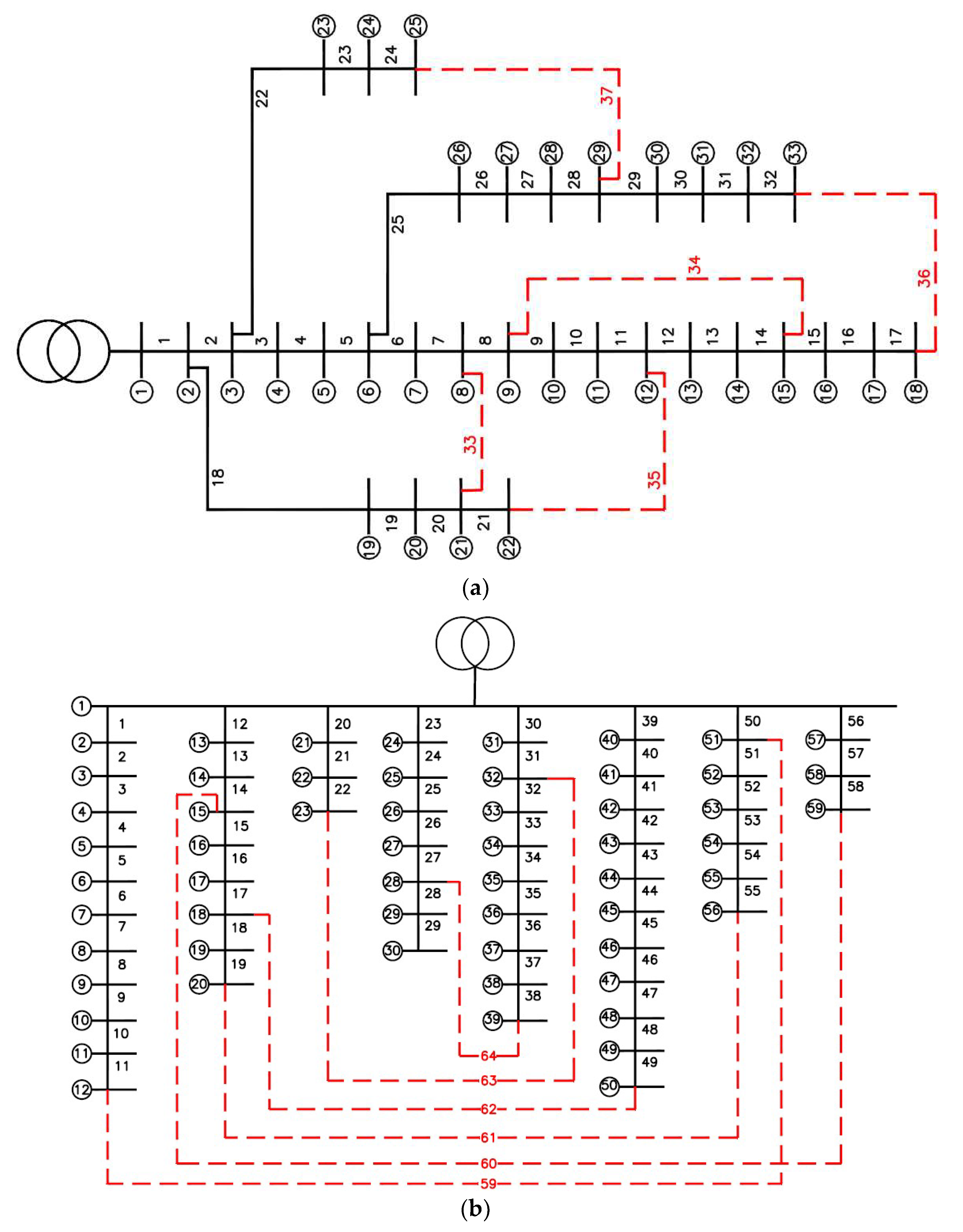
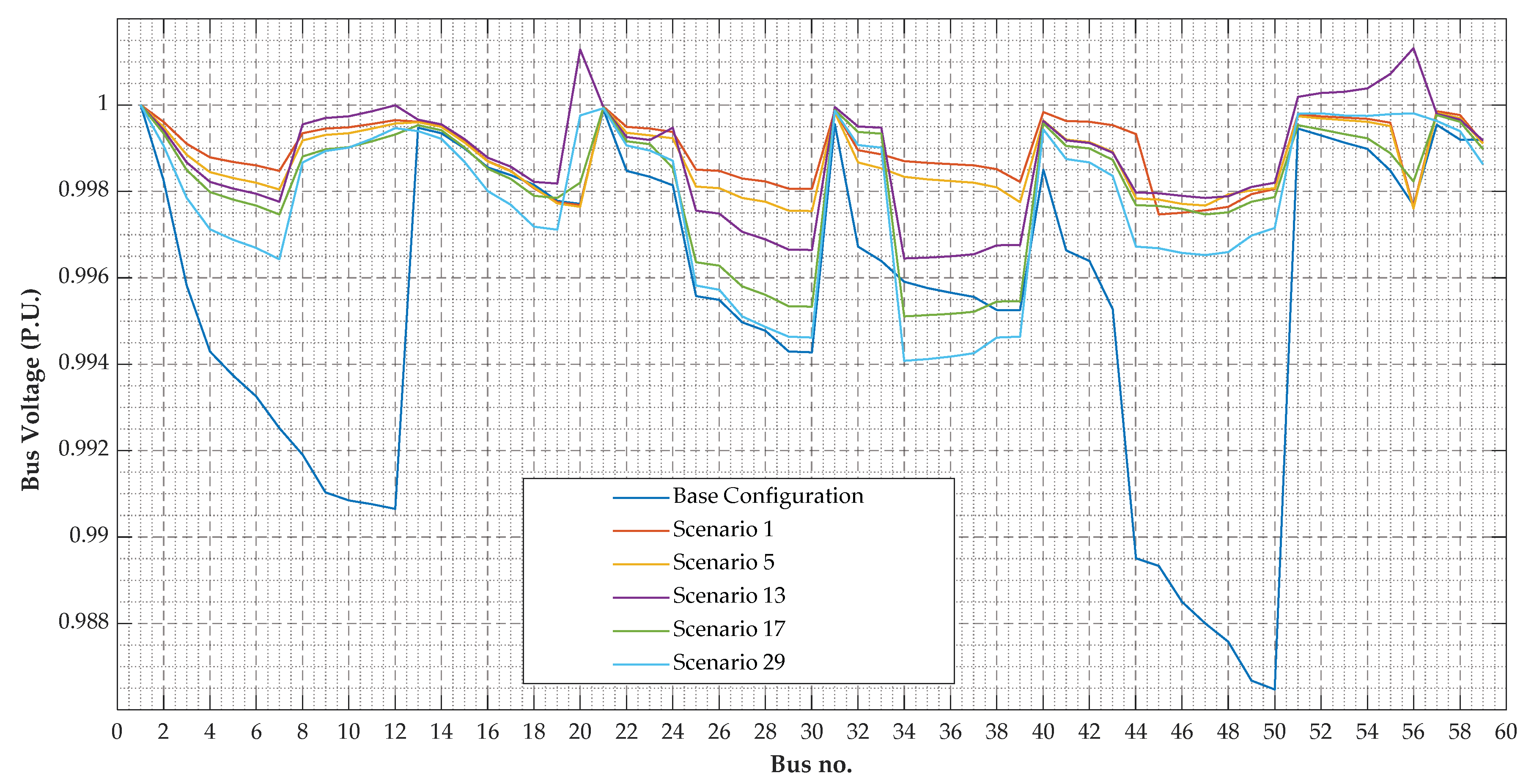
Case 1: In this case study, PV units and WTs, as the considered renewable DGs, are allocated at certain predetermined buses of the 59-bus distribution network as listed below in

Table 5. PV units and WTs buses of the 59-bus distribution network (Case 1).

Network	WTs Buses	PV Units Buses
59-bus	13,24,31,52,55,56	2,7,22,29,43,50

. The optimal sizing of these DGs is determined, using the SHADE algorithm, in addition to the optimal network configuration, considering different scenarios of load demand, wind speed and solar irradiance for maximizing the probabilistic hosting capacity (PHC) of the network, minimizing the network power losses (i.e., maximizing the reduced power losses), and improving the voltage profile. This case study is conducted in order to provide a feasible comparison with the previously presented study in [103] using multi-objective optimization techniques (NSGA-II, MOPSO, MOMVO and MOFPA). The obtained simulation results of this case study regarding the $PHC$, $R{P}_{loss}$ and voltage profile, in comparison to those presented in [103], are listed below in

Table 6. Simulation results of the first case study (Case 1).

Network	Index	Initial	NSGA-II	MOPSO	MOMVO	MOFPA	SHADE
59-bus	$PHC$ (%)	-	18.087	14.05	12.395	12.354	16.851
	$R{P}_{loss}$ (%)	-	83.3078	81.8076	72.859	81.169	93.995
	$AVD{I}_{ov}$	0.1407	0.0844	0.0847	-	-	0.0814
	min $\left|V_{k,s}\right|$ (p.u.)	0.9874	0.9944	0.9931	-	-	0.9938
	max $\left|V_{k,s}\right|$ (p.u.)	1	1.0004	1.0029	-	-	1.0013

. Optimal sizing of the allocated PV units and WTs, in MW, is provided below in

Table 7. Optimal sizing of PV units and WTs in MW (Case 1).

WTs Buses	WT Size (NSGA-II)	WT Size (MOPSO)	WT Size (SHADE)	PV Units Buses	PV Size (NSGA-II)	PV Size (MOPSO)	PV Size (SHADE)
13	1.7	1	3.3	2	2.4	2.1	3.1
24	5.5	1	0.58	7	2.8	4.4	3.9
31	1.7	1	0.91	22	2.3	2.9	1.8
52	2.1	1	2.2	29	1.4	1	1.9
55	2.8	1	3.0	43	2.2	0	4.1
56	2.3	1	2.5	50	1.7	12.2	1.7

. In addition, the tie-switches selected by the SOE method for the optimal network reconfiguration for various scenarios are supplied below in

Table 8. Selected tie-switches for optimal network configuration for various scenarios (Case 1).

Scenario No.	(Selected Tie-Switches)
	NSGA-II	MOPSO	SOE
1	7,18,46,60,63,64	7,19,46,60,63,64	9,31,38,45,55,60
5	7,17,47,60,63,64	7,18,46,60,63,64	7,47,55,58,63,64
13	7,17,37,47,60,63		11,18,37,47,58,63
17	7,17,38,48,60,63
29	7,18,38,46,60,63	7,18,38,46,60,63	11,21,37,47,55,58

. Finally, the voltage profile improvement after the optimal DG integration and network reconfiguration for various scenarios is shown below in Figure 3.

(b) 

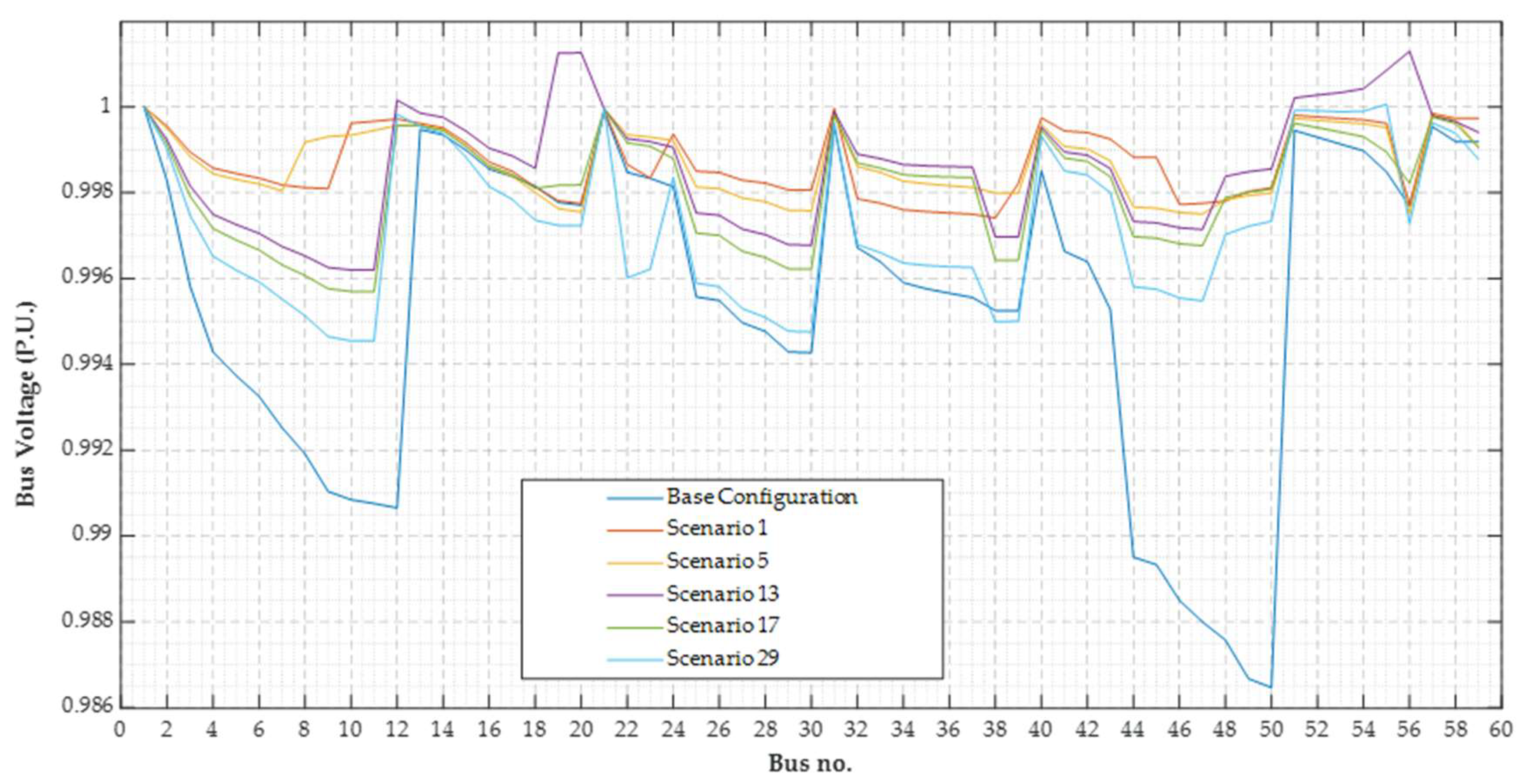
Case 2: In this case study, optimal allocation and sizing of two shunt capacitors in the considered 59-bus distribution network are added to the optimization problem of the previous case study (Case 1) to step on the effect of integrating SCs on system performance. The obtained simulation results of this case study regarding the $PHC$, $R{P}_{loss}$ and voltage profile are listed below in

Table 9. Simulation results of the second case study (Case 2).

Network	Index	Initial	SHADE (Case 1)	SHADE (Case 2)
59-bus	$PHC$ (%)	-	16.851	17.089
	$R{P}_{loss}$ (%)	0	93.995	95.299
	$AVD{I}_{ov}$	0.1407	0.0814	0.0724
	min$\left|V_{k,s}\right|$ (p.u.)	0.9874	0.9938	0.9932
	max $\left|V_{k,s}\right|$ (p.u.)	1	1.0013	1.0013

. Optimal locations and sizes of SCs, in MVAR, in the distribution network in addition to optimal sizing of the allocated PV units and WTs, in MW, are provided below in

Table 10. Optimal allocation and sizing of PV units, WTs and SCs in MW / MVAR (Case 2).

WTs Buses	WT Size (SHADE—Case 1)	WT Size (SHADE—Case 2)	PV Units Buses	PV Size (SHADE—Case 1)	PV Size (SHADE—Case 2)	SCs Buses	SC Size (SHADE—Case 2)
13	3.3	0.95	2	3.1	0.29	43	0.75
24	0.58	3.6	7	3.9	1.3	16	0.50
31	0.91	0.98	22	1.8	2.2	-	-
52	2.2	3.8	29	1.9	4.07	-	-
55	3.0	2.08	43	4.1	3.3	-	-
56	2.5	2.7	50	1.7	2.9	-	-

. Besides, the tie-switches selected by the SOE method for the optimal network reconfiguration, for various scenarios, are supplied below in

Table 11. Selected tie-switches for optimal network configuration for various scenarios (Case 2).

Scenario No.	(Selected Tie-Switches)
	SOE (Case 1)	SOE (Case 2)
1	9,31,38,45,55,60	7,38,44,55,58,63
5	7,47,55,58,63,64	7,38,47,55,58,63
13	11,18,37,47,58,63	7,19,33,46,58,63
17
29	11,21,37,47,55,58

. Finally, the voltage profile improvement after the optimal DG and SC integration and network reconfiguration for various scenarios is shown below in Figure 4.

(c) 

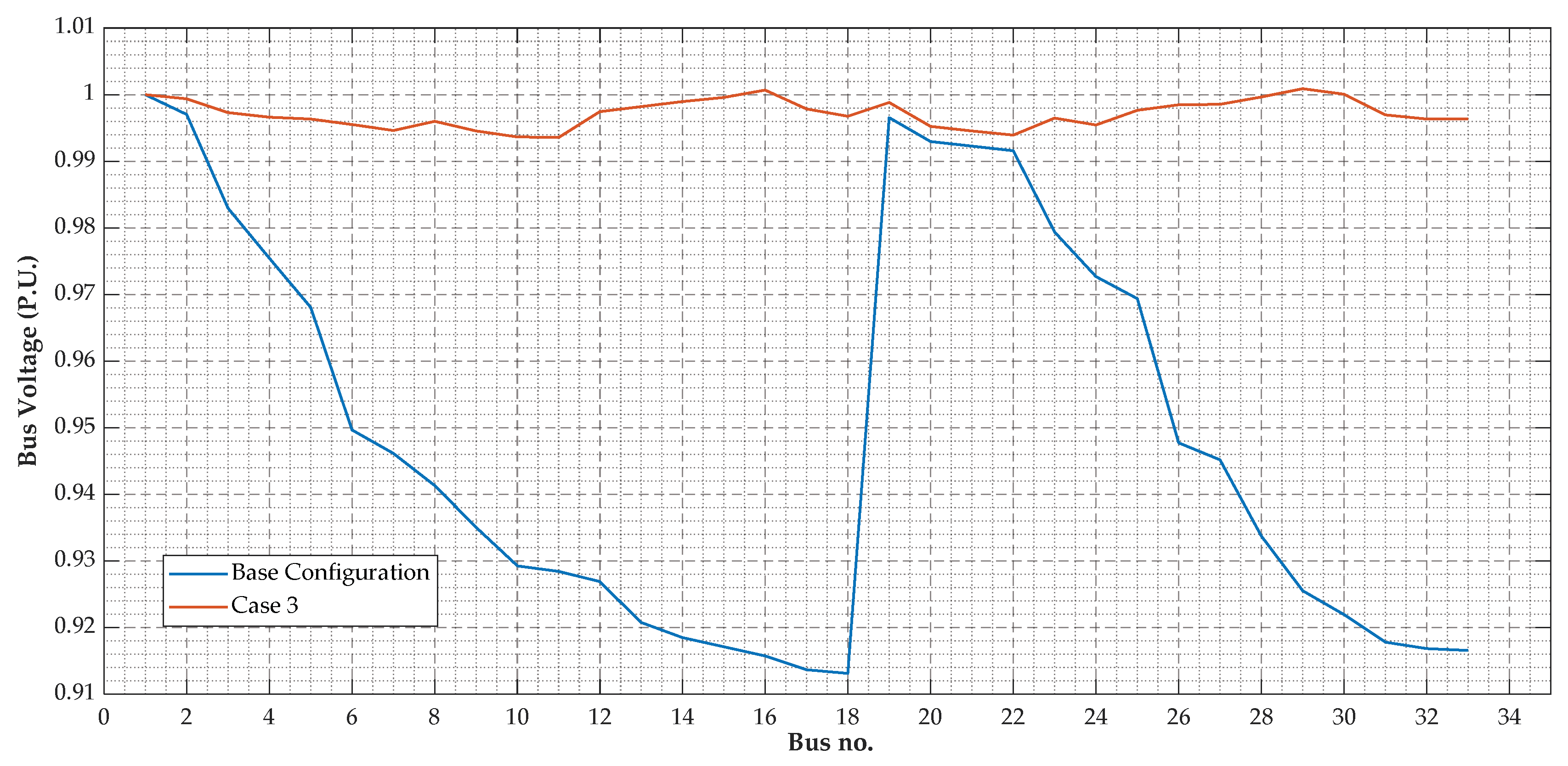
Case 3: In this case study, the optimal allocation and sizing of three DGs and three SCs in the considered 33-bus distribution network are determined, using the SHADE algorithm simultaneously with the optimal network configuration, using the SOE method, without considering the demand load variability or the DG output power uncertainty for minimizing network power loss and improving the voltage profile. The simulation results obtained from this case study are compared with those provided by the previously presented studies in [104,105], using the DE and the BPSO optimization algorithms, and listed below in

Table 12. Simulation results of the third case study (Case 3).

Network	Index	Initial	DE [104]	BPSO [105]	SHADE
33-bus	DGs Size (MW)	-	0.557 0.813 0.630	0.70 0.60 0.70	1.532 0.721 0.641
	Total allocated MW	-	2.00	2.00	2.89
	DGs location (Bus Number)	-	15,25,32	15,31,25	29,8,16
	SCs Size (MVAR)	-	0.703 0.399 1.198	0.382 1.013 0.419	1.260 0.236 0.197
	Total allocated MVAR	-	2.30	1.81	1.69
	SCs location (Bus Number)	-	3,9,30	14,30,24	30,14,2
	Selected tie-switches	33,34,35,36,37	7,11,12,17,26	7,35,10,36,26	11,25,33,34,35
	$P_{loss} \left(KW\right)$	202.66	15.63	15.47	12.70
	$R{P}_{loss}$ (%)	-	92.3	92.4	93.7
	min $\left|V_{k,s}\right|$ (p.u.)	0.9131	0.9891	0.9887	0.9936

. Voltage profile enhancement after the optimal DG and SC integration in addition to optimal network reconfiguration is shown below in Figure 5.

(d) 

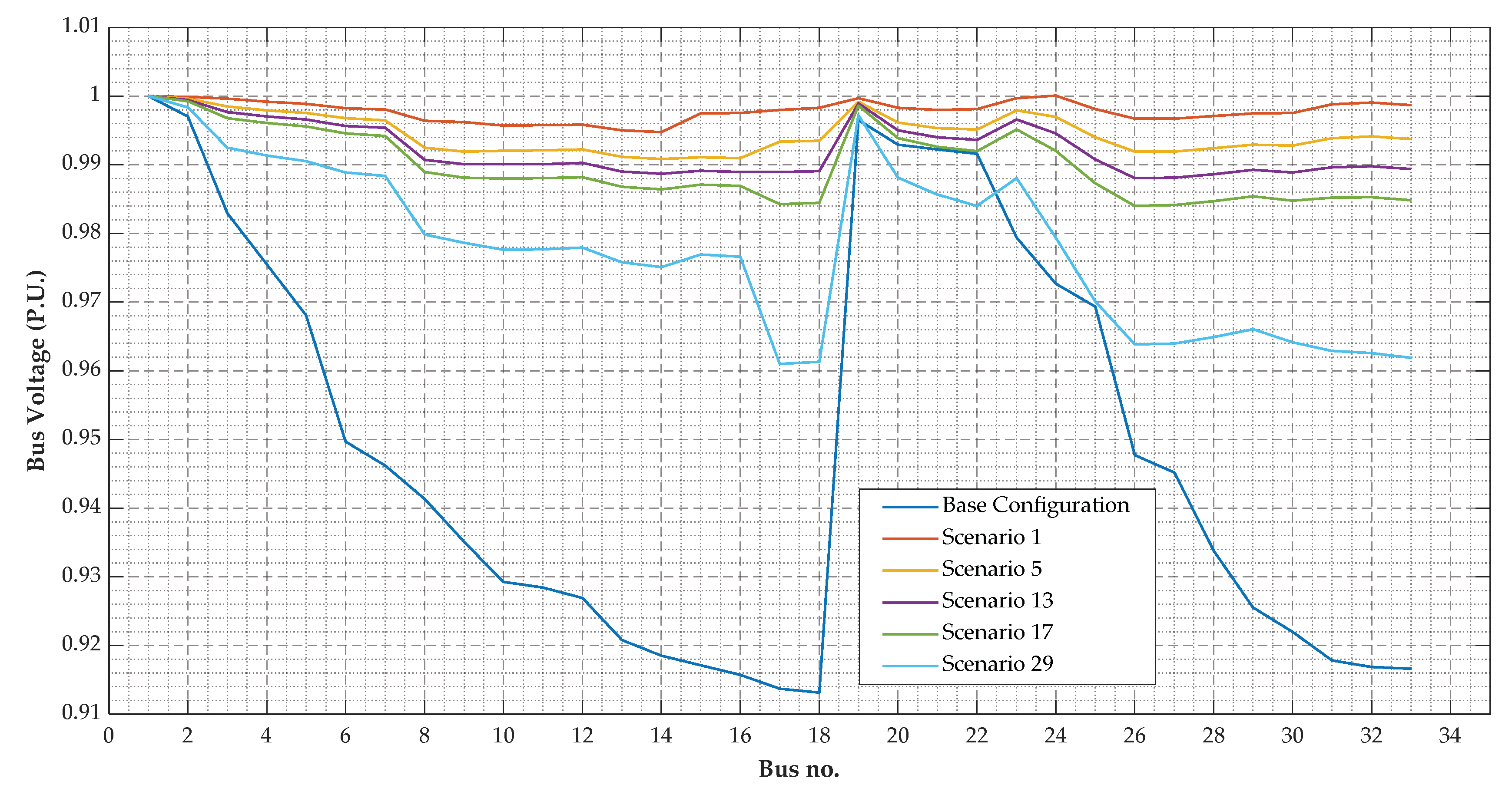
Case 4: In this case study, the variability or uncertainty associated with the network demand load is considered based on different loading scenarios, as indicated in Table 1, in solving the optimization problem of the previous case study (Case 3) in order to investigate the effect of considering realistic variable loads on the optimization results. The obtained simulation results of this case study are listed below in

Table 13. Simulation results of the fourth and fifth case studies (Cases 4 & 5).

Network	Index	Initial	SHADE (Case 3)	SHADE (Case 4)	SHADE (Case 5)
33-bus	DGs Size (MW)	-	1.532 0.721 0.641	0.403 0.360 0.279	0.701 0.503 0.30
	Total allocated MW	-	2.89	1.04	1.50
	DGs location (Bus Number)	-	29,8,16	32,24,22	24,20,30
	SCs Size (MVAR)	-	1.260 0.236 0.197	0.325 0.130 0.184	0.813 0.604 0.70
	Total allocated MVAR	-	1.69	0.639	2.12
	SCs location (Bus Number)	-	30,14,2	24,31,3	19,3,25
	Selected tie-switches	33,34,35,36,37	11,25,33,34,35	7,9,14,16,25	11,14,17,25,33
	$P_{loss} \left(KW\right)$	202.66	12.70	2.75	7.30
	$R{P}_{loss}$ (%)	-	93.7	98.6	96.4
	$\min \left|V_{k,s}\right|$ (p.u.)	0.9131	0.9936	0.9559	0.9521

. Voltage profile improvement after the optimal DG and SC integration in addition to optimal network reconfiguration is as depicted below in Figure 6.

(e) 

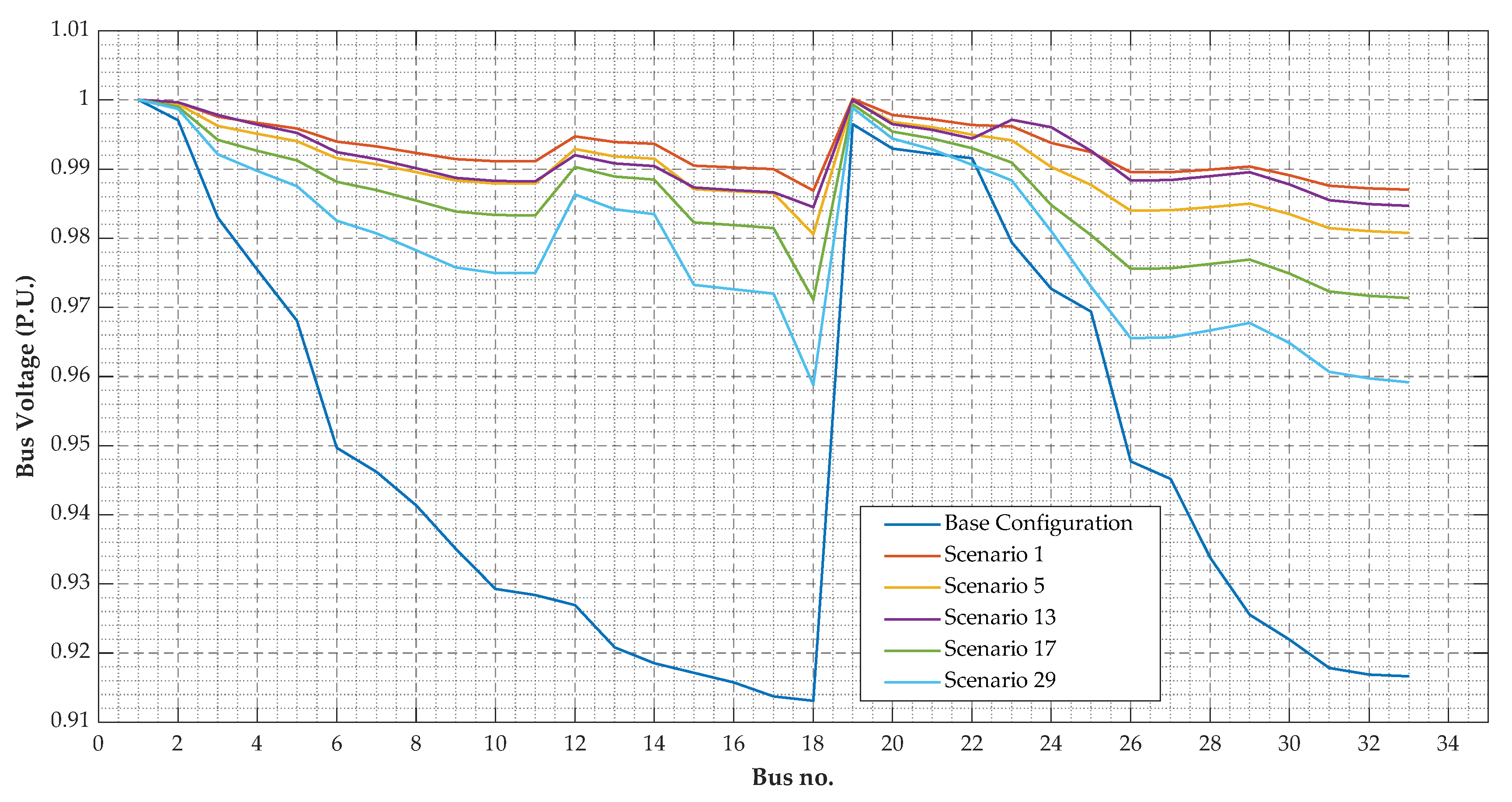
Case 5: In this case study, the variability or uncertainty associated with both the network demand load and DG output power is considered in solving the optimization problem of Case 3. One wind turbine and two PV units are considered as the DG units in this case study with different scenarios for wind speed and solar irradiance as listed in Table 1. This case study is performed to investigate the effect of realistic uncertain demand load and DG output power on optimization results. The obtained simulation results of this case study are provided below in Table 13. Voltage profile enhancement is shown below in Figure 7 after the optimal DG and SC integration along with optimal network reconfiguration.

For the problem of case 1, as shown above in Table 6 and Table 7, it has been found that using the SHADE optimization algorithm and the SOE reconfiguration technique for the different considered scenarios, the probabilistic hosting capacity ($PHC$) of the network reached 16.851%, the reduced network power losses reached 93.99%, while the voltage deviation index $\left(AVD{I}_{ov}\right)$ decreased to 0.0814. From Table 7, it can be noted that the optimal sizes of WTs allocated at buses 24 and 31 (0.58 MW and 0.91 MW), obtained using the SHADE algorithm, are less than those obtained using the NSGA-II algorithm (5.5 MW and 1.7 MW) and the MOPSO algorithm (1 MW for both WTs). Besides, the optimal sizes of PV units allocated at buses 7 and 50 (3.9 MW and 1.7 MW), obtained by the SHADE algorithm, are less than those obtained by the MOPSO algorithm (4.4 MW and 12.2 MW), while the obtained optimal size of the PV unit allocated at bus 22 (1.8 MW), using the SHADE algorithm, is less than that obtained using both the NSGA-II algorithm (2.3 MW) and the MOPSO algorithm (2.9 MW). Despite that, the optimal sizes of PV units and WTs at certain buses of the network, obtained by the SHADE algorithm, are less than those obtained using other techniques as indicated above; the employed SHADE optimization algorithm, in association with the SOE reconfiguration method, achieves PHC of 16.85%, which is almost touching that provided by the NSGA-II algorithm (18.08%) and it exceeds that achieved using MOPSO, MOMVO, and MOFPA algorithms. It is also notable, from Table 6, that the SHADE and the SOE methods achieve the maximum reduced power losses (93.995%) which surpasses the values provided using NSGA-II, MOPSO, MOMVO, and MOFPA algorithms by 10.7%, 12.2%, 21.1%, and 12.8%, respectively. In addition, the NSGA-II algorithm achieves the maximum value for the minimum bus voltage (0.9944 p.u.), then the SHADE algorithm (0.9938 p.u.), then the MOPSO algorithm (0.9931 p.u.), while the MOPSO algorithm achieves the maximum value for the maximum bus voltage (1.0029 p.u.), then the SHADE algorithm (1.0013 p.u.), then the NSGA-II algorithm (1.0004 p.u.). However, the SHADE algorithm, along with the SOE method, achieves the best (lowest) value for the overall aggregated voltage deviation index (0.0814). In view of those aforementioned results, it can be stated that the SHADE optimization algorithm and the SOE reconfiguration method provide the best performance and solutions, compared to other techniques, which indicates their effectiveness and their superiority for solving the considered optimization problem. The effect of adding optimal allocation and sizing of SCs to the optimization problem of case 1 has been investigated in the second case study (case 2) and the results, listed in Table 9 and Table 10, indicate that optimal integration of SCs and DGs with the optimal sizes and locations listed in Table 10, simultaneously with the optimal network reconfiguration, lead to increasing the network PHC to be 17.1% instead of 16.85% provided in the first case study (without SCs), increasing the reduced network power losses ($R{P}_{loss}$) to 95.3% instead of 93.9% and decreasing the voltage deviation index $\left(AVD{I}_{ov}\right)$ to 0.0724 instead of 0.0814. It can be noted that the optimal sizes of WTs allocated at buses 13 and 55 (0.95 MW and 2.08 MW), in case 2, are less than those obtained in case 1 (3.3 MW and 3 MW). Besides, the optimal sizes of PV units allocated at buses 2, 7, and 43 (0.29 MW, 1.3 MW and 3.3 MW), in case 2, are less than those obtained in case 1 (3.1 MW, 3.9 MW and 4.1 MW). However, the network PHC obtained in case 2 (17.089%) is larger than that obtained in case 1 (16.851%). It is also notable that despite the minimum bus voltage obtained from case 1 being slightly less than that obtained in case 2, the aggregated voltage deviation index $\left(AVD{I}_{ov}\right)$ obtained in case 2 is less than that obtained in case 1. Hence, it can be concluded that optimal integration of SCs in addition to DGs and network reconfiguration has a positive effect on improving system performance. For the problem of case 3, as listed in Table 12, it has been found that using the SHADE algorithm along with the SOE method, minimum network power losses were achieved (12.7 kW) compared to other techniques, namely DE (15.63 kW) and BPSO (15.47 kW). In other words, the SHADE algorithm in association with the SOE method provide the maximum reduced power loss (93.7%) compared to DE (92.3%) and BPSO (92.4%). It can also be noted that the SHADE algorithm provides the maximum value for the minimum bus voltage (0.9936 p.u.) compared to DE (0.9891 p.u.) and BPSO (0.9887 p.u.). Those demonstrated results in Table 12 indicate the efficiency and the effectiveness of the employed SHADE algorithm and the SOE method in addition to their superiority over other used techniques for solving the considered optimization problem. The obtained simulation results of cases 4 and 5, as indicated above in Table 13, show that considering the variability and uncertainty associated with the network demand load and DG output power in solving the optimization problem of case 3 has a major effect on the optimization results which notably differ from those obtained in case 3 (without considering uncertainties). In case 4, the obtained network power loss (probabilistic power losses) decreased to 2.75 kW (98.6% power loss reduction) with the optimally integrated DGs and SCs of total capacity 1.04 MW and 0.64 MVAR; respectively, while in case 5 the obtained network power loss has decreased to 7.30 kW (96.4% power loss reduction) with optimally integrated DGs and SCs of total capacity 1.50 MW and 2.12 MVAR, respectively, instead of 12.7 kW obtained power loss (93.7% power loss reduction) with optimally integrated DGs (2.89 MW total allocated capacity) and SCs (1.69 MVAR total allocated capacity) in case 3, where the uncertainties are neglected. The aforementioned results of cases 4 and 5, in comparison to those of case 3, highlight the importance and effect of considering the uncertainties related to network load and DG output power for realistic modeling of the considered optimization problem and obtaining optimal solutions for the different network operational scenarios [106].

7. Conclusions and Future Works

In the work presented in this paper, the SHADE optimization algorithm has been employed for optimal integration of renewable DGs (WTs and PV units) and shunt capacitors in the considered distribution networks, simultaneously with the optimal network reconfiguration using the SOE method and with consideration of demand load and DG output power uncertainties. Optimization objectives have included maximizing the probabilistic hosting capacity of the network, minimizing the network power losses, and enhancing the voltage profile. Five different case studies were conducted, considering the real 59-bus distribution network of Cairo and the 33-bus test distribution network. The first case study has discussed optimal DG integration simultaneously with optimal network reconfiguration for the 59-bus distribution network and considering load and DG output uncertainties. The employed SHADE algorithm and the SOE method have provided maximum hosting capacity (16.851%) and reduced power losses (93.99%) as well as minimum voltage deviation index (0.0814) compared to techniques presented in other previous literature [103]—as indicated in Table 6, which validates their effectiveness and superiority. The second case study has investigated the effect of adding SC integration to the optimization problem of the first case study, which is the main contribution of this paper. As shown in Table 9, SC integration has led to improving (increasing) hosting capacity (17.1%) and reduced power loss (95.3%) in addition to further improvement of the voltage profile with an improved (reduced) voltage deviation index (0.0724). The third case study presented optimal integration of DGs and SCs in the 33-bus distribution network, simultaneously with the network reconfiguration and without considering the uncertainties related to demand load and DG output. The employed SHADE algorithm and the SOE method, as listed in Table 12, provided the best results, compared to other techniques used in previously presented research [104,105] regarding power loss reduction (93.7% compared to 92.3% and 92.4%) and voltage profile improvement (0.994 min. bus voltage compared to 0.989 and 0.988). The fourth and fifth case studies investigated the effect of considering uncertainties related to network load and DG output power in solving the optimization problem of case 3. These case studies also reflect the main contribution of the work presented in this paper as the optimal integration of DGs and SCs, simultaneously with network reconfiguration and with consideration of demand load and DG output uncertainty, hasn’t been presented in the available literature. The obtained results, as depicted in Table 13, have indicated the major effect of considering such uncertainties on the optimization results to provide optimal solution for the different network operational scenarios with realistic modeling of the considered optimization problem. There are some aspects that haven’t been considered in work presented within this research and can be addressed in future works. These aspects include integration of a suitable type energy storage system (ESS) into the considered distribution network to support the renewable DGs in case of low or zero output power, in addition to investigating the effect on system performance. Besides, system reliability assessment and considering other indices for evaluating distribution system performance. Future works could also include considering other distribution networks with larger scale and employing other optimization techniques with a comparative study between different considered techniques.

References

1. Tuballa, M.L.; Abundo, M.L. A review of the development of Smart Grid technologies. Renew. Sustain. Energy Rev. 2016, 59, 710–725. [Google Scholar] [CrossRef]
2. Viawan, F. Voltage Control and Voltage Stability of Power Distribution Systems in the Presence of Distributed Generation; Chalmers Tekniska Hogskola: Göteborg, Sweden, 2008. [Google Scholar]
3. El-Khattam, W.; Salama, M.M. Distributed generation technologies, definitions and benefits. Electr. Power Syst. Res. 2004, 71, 119–128. [Google Scholar] [CrossRef]
4. Available online: https://www.matec-conferences.org/articles/matecconf/pdf/2016/01/matecconf_ses2016_01007.pdf (accessed on 15 February 2022).
5. Prakash, P.; Khatod, D.K. Optimal sizing and siting techniques for distributed generation in distribution systems: A review. Renew. Sustain. Energy Rev. 2016, 57, 111–130. [Google Scholar] [CrossRef]
6. Ganguly, S.; Sahoo, N.C.; Das, D. A novel multi-objective PSO for electrical distribution system planning incorporating distributed generation. Energy Syst. 2010, 1, 291–337. [Google Scholar] [CrossRef]
7. Griffin, T.; Tomsovic, K.; Secrest, D.; Law, A. Placement of dispersed generation systems for reduced losses. In Proceedings of the 33rd Annual Hawaii International Conference on System Sciences, Maui, HI, USA, 7 January 2000. [Google Scholar]
8. Gampa, S.R.; Das, D. Optimum placement and sizing of DGs considering average hourly variations of load. Int. J. Electr. Power Energy Syst. 2015, 66, 25–40. [Google Scholar] [CrossRef]
9. Kanwar, N.; Gupta, N.; Niazi, K.R.; Swarnkar, A.; Bansal, R. Simultaneous allocation of distributed energy resource using improved particle swarm optimization. Appl. Energy 2017, 185, 1684–1693. [Google Scholar] [CrossRef]
10. Reddy, P.S.; Babu, K.; Reddy, K.H. Optimal Location and Size of Distributed Generations Using Kalman Filter Algorithm for Reduction of Power Loss and Voltage Profile Improvement. Int. J. Eng. Res. Dev. 2014, 10, 19–28. [Google Scholar]
11. Hlaing, C.S.; Swe, P.L. Effects of Distributed Generation on System Power Losses and Voltage Profiles (Belin Distribution System). J. Electr. Electron. Eng. 2015, 3, 36. [Google Scholar] [CrossRef]
12. Shukla, T.N.; Singh, S.P.; Srinivasarao, V.; Naik, K.B. Optimal Sizing of Distributed Generation Placed on Radial Distribution Systems. Electr. Power Components Syst. 2010, 38, 260–274. [Google Scholar] [CrossRef]
13. Gnanambal, K.; Suriya, S. Optimal Sizing Of Distributed Generation For Voltage Profile Improvement Considering Maximum Loadability Limit. Int. J. Innov. Res. Sci. Eng. Technol. 2014, 3, 304–309. [Google Scholar]
14. Szuvovivski, I.; Fernandes, T.; Aoki, A. Simultaneous allocation of capacitors and voltage regulators at distribution networks using Genetic Algorithms and Optimal Power Flow. Int. J. Electr. Power Energy Syst. 2012, 40, 62–69. [Google Scholar] [CrossRef]
15. Gampa, S.R.; Das, D. Optimum placement of shunt capacitors in a radial distribution system for substation power factor improvement using fuzzy GA method. Int. J. Electr. Power Energy Syst. 2016, 77, 314–326. [Google Scholar] [CrossRef]
16. Luis, G.N.; Victor, G.A. Optimal Location and Sizing of Capacitors in Radial Distribution Networks Using an Exact MINLP Model for Operating Costs Minimization. 2017. Available online: http://repositorio.utb.edu.co/handle/20.500.12585/8966 (accessed on 15 February 2022).
17. Mohammadi, M. Particle swarm optimization algorithm for simultaneous optimal placement and sizing of shunt active power conditioner (APC) and shunt capacitor in harmonic distorted distribution system. J. Central South Univ. 2017, 24, 2035–2048. [Google Scholar] [CrossRef]
18. Taha, I.B.M.; Elattar, E.E. Optimal reactive power resources sizing for power system operations enhancement based on improved grey wolf optimiser. IET Gener. Transm. Distrib. 2018, 12, 3421–3434. [Google Scholar] [CrossRef]
19. Sajjadi, S.M.; Haghifam, M.-R.; Salehi, J. Simultaneous placement of distributed generation and capacitors in distribution networks considering voltage stability index. Int. J. Electr. Power Energy Syst. 2013, 46, 366–375. [Google Scholar] [CrossRef]
20. Moradi, M.H.; Zeinalzadeh, A.; Mohammadi, Y.; Abedini, M. An efficient hybrid method for solving the optimal sitting and sizing problem of DG and shunt capacitor banks simultaneously based on imperialist competitive algorithm and genetic algorithm. Int. J. Electr. Power Energy Syst. 2014, 54, 101–111. [Google Scholar] [CrossRef]
21. Jain, N.; Singh, S.; Srivastava, S. PSO based placement of multiple wind DGs and capacitors utilizing probabilistic load flow model. Swarm Evol. Comput. 2014, 19, 15–24. [Google Scholar] [CrossRef]
22. Naik, S.G.; Khatod, D.; Sharma, M. Optimal allocation of combined DG and capacitor for real power loss minimization in distribution networks. Int. J. Electr. Power Energy Syst. 2013, 53, 967–973. [Google Scholar] [CrossRef]
23. Zeinalzadeh, A.; Mohammadi, Y.; Moradi, M.H. Optimal multi objective placement and sizing of multiple DGs and shunt capacitor banks simultaneously considering load uncertainty via MOPSO approach. Int. J. Electr. Power Energy Syst. 2015, 67, 336–349. [Google Scholar] [CrossRef]
24. Kanwar, N.; Gupta, N.; Niazi, K.R.; Swarnkar, A. Improved meta-heuristic techniques for simultaneous capacitor and DG allocation in radial distribution networks. Int. J. Electr. Power Energy Syst. 2015, 73, 653–664. [Google Scholar] [CrossRef]
25. Khan, N.A.; Ghoshal, S.P.; Ghosh, S. Optimal Allocation of Distributed Generation and Shunt Capacitors for the Reduction of Total Voltage Deviation and Total Line Loss in Radial Distribution Systems Using Binary Collective Animal Behavior Optimization Algorithm. Electr. Power Components Syst. 2014, 43, 119–133. [Google Scholar] [CrossRef]
26. Ghaffarzadeh, N.; Sadeghi, H. A new efficient BBO based method for simultaneous placement of inverter-based DG units and capacitors considering harmonic limits. Int. J. Electr. Power Energy Syst. 2016, 80, 37–45. [Google Scholar] [CrossRef]
27. Khodabakhshian, A.; Andishgar, M.H. Simultaneous placement and sizing of DGs and shunt capacitors in distribution systems by using IMDE algorithm. Int. J. Electr. Power Energy Syst. 2016, 82, 599–607. [Google Scholar] [CrossRef]
28. Rahmani-Andebili, M. Simultaneous placement of DG and capacitor in distribution network. Electr. Power Syst. Res. 2016, 131, 1–10. [Google Scholar] [CrossRef]
29. Kayal, P.; Chanda, C.K. Strategic approach for reinforcement of intermittent renewable energy sources and capacitor bank for sustainable electric power distribution system. Int. J. Electr. Power Energy Syst. 2016, 83, 335–351. [Google Scholar] [CrossRef]
30. Khan, N.A.; Ghosh, S.; Ghoshal, S.P. Optimal allocation and sizing of DG and shunt capacitors using differential evolutionary algorithm. Int. J. Power Energy Convers. 2013, 4, 278. [Google Scholar] [CrossRef]
31. Dixit, M.; Kundu, P.; Jariwala, H.R. Incorporation of distributed generation and shunt capacitor in radial distribution system for techno-economic benefits. Eng. Sci. Technol. Int. J. 2017, 20, 482–493. [Google Scholar] [CrossRef]
32. Mohamed, E.; Mohamed, A.-A.A.; Mitani, Y. Hybrid GMSA for Optimal Placement and Sizing of Distributed Generation and Shunt Capacitors. J. Eng. Sci. Technol. Rev. 2018, 11, 55–65. [Google Scholar] [CrossRef]
33. Baziareh, A.; Kavousi-Fard, F.; Zare, A.; Abasizade, A.; Saleh, S. Stochastic reactive power planning in distribution systems considering wind turbines electric power variations. J. Intell. Fuzzy Syst. 2015, 28, 1081–1087. [Google Scholar] [CrossRef]
34. Rajendran, A.; Narayanan, K. Optimal multiple installation of DG and capacitor for energy loss reduction and loadability enhancement in the radial distribution network using the hybrid WIPSO–GSA algorithm. Int. J. Ambient. Energy 2018, 41, 129–141. [Google Scholar] [CrossRef]
35. Pereira, B.R.; Da Costa, G.R.M.M.; Contreras, J.; Mantovani, J.R.S. Optimal Distributed Generation and Reactive Power Allocation in Electrical Distribution Systems. IEEE Trans. Sustain. Energy 2016, 7, 975–984. [Google Scholar] [CrossRef] [Green Version]
36. Niknam, T.; Fard, A.K.; Seifi, A.R. Distribution feeder reconfiguration considering fuel cell/wind/photovoltaic power plants. Renew. Energy 2012, 37, 213–225. [Google Scholar] [CrossRef]
37. Savier, J.; Das, D. Loss allocation to consumers before and after reconfiguration of radial distribution networks. Int. J. Electr. Power Energy Syst. 2011, 33, 540–549. [Google Scholar] [CrossRef]
38. Sultana, B.; Mustafa, M.; Sultana, U.; Bhatti, A.R. Review on reliability improvement and power loss reduction in distribution system via network reconfiguration. Renew. Sustain. Energy Rev. 2016, 66, 297–310. [Google Scholar] [CrossRef]
39. Nguyen, T.T.; Truong, A.V. Distribution network reconfiguration for power loss minimization and voltage profile improvement using cuckoo search algorithm. Int. J. Electr. Power Energy Syst. 2015, 68, 233–242. [Google Scholar] [CrossRef]
40. Kavousi-Fard, A.; Niknam, T. Multi-objective stochastic Distribution Feeder Reconfiguration from the reliability point of view. Energy 2014, 64, 342–354. [Google Scholar] [CrossRef]
41. Aman, M.; Jasmon, G.; Bakar, A.; Mokhlis, H. Optimum network reconfiguration based on maximization of system loadability using continuation power flow theorem. Int. J. Electr. Power Energy Syst. 2014, 54, 123–133. [Google Scholar] [CrossRef]
42. Kalambe, S.; Agnihotri, G. Loss minimization techniques used in distribution network: Bibliographical survey. Renew. Sustain. Energy Rev. 2014, 29, 184–200. [Google Scholar] [CrossRef]
43. López, J.C.; Lavorato, M.; Rider, M.J. Optimal reconfiguration of electrical distribution systems considering reliability indices improvement. Int. J. Electr. Power Energy Syst. 2016, 78, 837–845. [Google Scholar] [CrossRef]
44. Paterakis, N.G.; Mazza, A.; Santos, S.F.; Erdinç, O.; Chicco, G.; Bakirtzis, A.G.; Catalão, J.P. Multi-objective reconfiguration of radial distribution systems using reliability indices. IEEE Trans. Power Syst. 2015, 31, 1048–1062. [Google Scholar] [CrossRef]
45. Ch, Y.; Goswami, S.; Chatterjee, D. Effect of network reconfiguration on power quality of distribution system. Int. J. Electr. Power Energy Syst. 2016, 83, 87–95. [Google Scholar] [CrossRef]
46. Narimani, M.R.; Vahed, A.A.; Azizipanah-Abarghooee, R.; Javidsharifi, M. Enhanced gravitational search algorithm for multi-objective distribution feeder reconfiguration considering reliability, loss and operational cost. IET Gener. Transm. Distrib. 2014, 8, 55–69. [Google Scholar] [CrossRef]
47. Azizivahed, A.; Narimani, H.; Naderi, E.; Fathi, M.; Narimani, M.R. A hybrid evolutionary algorithm for secure multi-objective distribution feeder reconfiguration. Energy 2017, 138, 355–373. [Google Scholar] [CrossRef]
48. Liu, Y.; Li, J.; Wu, L. Coordinated Optimal Network Reconfiguration and Voltage Regulator/DER Control for Unbalanced Distribution Systems. IEEE Trans. Smart Grid 2018, 10, 2912–2922. [Google Scholar] [CrossRef]
49. Peng, C.; Xu, L.; Gong, X.; Sun, H.; Pan, L. Molecular Evolution Based Dynamic Reconfiguration of Distribution Networks With DGs Considering Three-Phase Balance and Switching Times. IEEE Trans. Ind. Inform. 2019, 15, 1866–1876. [Google Scholar] [CrossRef]
50. Arif, A.; Wang, Z.; Wang, J.; Chen, C. Power Distribution System Outage Management With Co-Optimization of Repairs, Reconfiguration, and DG Dispatch. IEEE Trans. Smart Grid 2018, 9, 4109–4118. [Google Scholar] [CrossRef]
51. Takenobu, Y.; Yasuda, N.; Kawano, S.; Minato, S.-I.; Hayashi, Y. Evaluation of Annual Energy Loss Reduction Based on Reconfiguration Scheduling. IEEE Trans. Smart Grid 2016, 9, 1986–1996. [Google Scholar] [CrossRef]
52. Wang, H.; Zhang, W.; Liu, Y. A Robust Measurement Placement Method for Active Distribution System State Estimation Considering Network Reconfiguration. IEEE Trans. Smart Grid 2016, 9, 1. [Google Scholar] [CrossRef]
53. Singh, J.; Tiwari, R. Real power loss minimization of smart grid with electric vehicles using distribution feeder reconfiguration. IET Gener. Transm. Distrib. 2019, 13, 4249–4261. [Google Scholar] [CrossRef]
54. Jabr, R.A.; Dzafic, I.; Huseinagic, I. Real Time Optimal Reconfiguration of Multiphase Active Distribution Networks. IEEE Trans. Smart Grid 2017, 9, 6829–6839. [Google Scholar] [CrossRef]
55. Roberge, V.; Tarbouchi, M.; Okou, F.A. Distribution System Optimization on Graphics Processing Unit. IEEE Trans. Smart Grid 2015, 8, 1689–1699. [Google Scholar] [CrossRef]
56. Fonseca, A.G.; Tortelli, O.L.; Lourenço, E.M. Extended fast decoupled power flow for reconfiguration networks in distribution systems. IET Gener. Transm. Distrib. 2018, 12, 6033–6040. [Google Scholar] [CrossRef]
57. Khodayifar, S.; Raayatpanah, M.A.; Rabiee, A.; Rahimian, H.; Pardalos, P.M. Optimal Long-Term Distributed Generation Planning and Reconfiguration of Distribution Systems: An Accelerating Benders’ Decomposition Approach. J. Optim. Theory Appl. 2018, 179, 283–310. [Google Scholar] [CrossRef]
58. Khodr, H.M.; Martínez-Crespo, J.; Vale, Z.A.; Ramos, C. Optimal methodology for distribution systems reconfiguration based on OPF and solved by decomposition technique. Eur. Trans. Electr. Power 2010, 20, 730–746. [Google Scholar] [CrossRef] [Green Version]
59. Takenobu, Y.; Yasuda, N.; Minato, S.-I.; Hayashi, Y. Scalable enumeration approach for maximizing hosting capacity of distributed generation. Int. J. Electr. Power Energy Syst. 2019, 105, 867–876. [Google Scholar] [CrossRef]
60. Capitanescu, F.; Ochoa, L.; Margossian, H.; Hatziargyriou, N.D. Assessing the Potential of Network Reconfiguration to Improve Distributed Generation Hosting Capacity in Active Distribution Systems. IEEE Trans. Power Syst. 2015, 30, 346–356. [Google Scholar] [CrossRef]
61. Ramos, E.R.; Expósito, A.G.; Santos, J.R.; Iborra, F.L. Path-based distribution network modeling: Application to reconfiguration for loss reduction. IEEE Trans. Power Syst. 2005, 20, 556–564. [Google Scholar] [CrossRef]
62. Asrari, A.; Wu, T.; Lotfifard, S. The Impacts of Distributed Energy Sources on Distribution Network Reconfiguration. IEEE Trans. Energy Convers. 2016, 31, 606–613. [Google Scholar] [CrossRef]
63. Lavorato, M.; Franco, J.F.; Rider, M.J.; Romero, R. Imposing Radiality Constraints in Distribution System Optimization Problems. IEEE Trans. Power Syst. 2012, 27, 172–180. [Google Scholar] [CrossRef]
64. Ding, F.; Loparo, K.A. Hierarchical Decentralized Network Reconfiguration for Smart Distribution Systems—Part II: Applications to Test Systems. IEEE Trans. Power Syst. 2014, 30, 744–752. [Google Scholar] [CrossRef]
65. Jabr, R.; Singh, R.; Pal, B. Minimum Loss Network Reconfiguration Using Mixed-Integer Convex Programming. IEEE Trans. Power Syst. 2012, 27, 1106–1115. [Google Scholar] [CrossRef]
66. DE Souza, S.S.F.; Romero, R.; Pereira, J.; Saraiva, J.T. Artificial immune algorithm applied to distribution system reconfiguration with variable demand. Int. J. Electr. Power Energy Syst. 2016, 82, 561–568. [Google Scholar] [CrossRef] [Green Version]
67. Yin, S.-A.; Lu, C.-N. Distribution Feeder Scheduling Considering Variable Load Profile and Outage Costs. IEEE Trans. Power Syst. 2009, 24, 652–660. [Google Scholar] [CrossRef]
68. Chen, C.-S.; Cho, M.-Y. Energy loss reduction by critical switches. IEEE Trans. Power Deliv. 1993, 8, 1246–1253. [Google Scholar] [CrossRef]
69. Golshannavaz, S.; Afsharnia, S.; Aminifar, F. Smart Distribution Grid: Optimal Day-Ahead Scheduling With Reconfigurable Topology. IEEE Trans. Smart Grid 2014, 5, 2402–2411. [Google Scholar] [CrossRef]
70. Jin, X.; Mu, Y.; Jia, H.; Wu, J.; Xu, X.; Yu, X. Optimal day-ahead scheduling of integrated urban energy systems. Appl. Energy 2016, 180, 1–13. [Google Scholar] [CrossRef] [Green Version]
71. Dorostkar-Ghamsari, M.R.; Fotuhi-Firuzabad, M.; Lehtonen, M.; Safdarian, A. Value of Distribution Network Reconfiguration in Presence of Renewable Energy Resources. IEEE Trans. Power Syst. 2016, 31, 1879–1888. [Google Scholar] [CrossRef]
72. Zidan, A.; El-Saadany, E.F. Distribution system reconfiguration for energy loss reduction considering the variability of load and local renewable generation. Energy 2013, 59, 698–707. [Google Scholar] [CrossRef]
73. Haghighat, H.; Zeng, B. Distribution System Reconfiguration under Uncertain Load and Renewable Generation. IEEE Trans. Power Syst. 2016, 31, 2666–2675. [Google Scholar] [CrossRef]
74. Ben Hamida, I.; Salah, S.B.; Msahli, F.; Mimouni, M.F. Optimal network reconfiguration and renewable DG integration considering time sequence variation in load and DGs. Renew. Energy 2018, 121, 66–80. [Google Scholar] [CrossRef]
75. Kianmehr, E.; Nikkhah, S.; Rabiee, A. Multi-objective stochastic model for joint optimal allocation of DG units and network reconfiguration from DG owner’s and DisCo’s perspectives. Renew. Energy 2019, 132, 471–485. [Google Scholar] [CrossRef]
76. Franco, J.F.; Rider, M.J.; Lavorato, M.; Romero, R. A mixed-integer LP model for the reconfiguration of radial electric distribution systems considering distributed generation. Electr. Power Syst. Res. 2013, 97, 51–60. [Google Scholar] [CrossRef]
77. Rosseti, G.J.; de Oliveira, E.J.; de Oliveira, L.W.; Silva, I.C., Jr.; Peres, W. Optimal allocation of distributed generation with reconfiguration in electric distribution systems. Electr. Power Syst. Res. 2013, 103, 178–183. [Google Scholar] [CrossRef]
78. Zidan, A.; Shaaban, M.; El-Saadany, E.F. Long-term multi-objective distribution network planning by DG allocation and feeders’ reconfiguration. Electr. Power Syst. Res. 2013, 105, 95–104. [Google Scholar] [CrossRef]
79. Rao, R.S.; Ravindra, K.; Satish, K.; Narasimham, S.V.L. Power Loss Minimization in Distribution System Using Network Reconfiguration in the Presence of Distributed Generation. IEEE Trans. Power Syst. 2013, 28, 317–325. [Google Scholar] [CrossRef]
80. Mirazimi, S.; Nematollahi, M.; Ashourian, M.; Mirahmadi, S. Reconfiguration and DG placement considering critical system condition. In Proceedings of the 2013 IEEE 7th International Power Engineering and Optimization Conference (PEOCO2013), Langkawi, Malaysia, 3–4 June 2013; pp. 676–679. [Google Scholar]
81. Pavani, P.; Singh, S.N. Reconfiguration of radial distribution networks with distributed generation for reliability improvement and loss minimization. In Proceedings of the 2013 IEEE Power & Energy Society General Meeting, Vancouver, BC, Canada, 21–25 July 2013; pp. 1–5. [Google Scholar]
82. Su, C.-T.; Lee, C.-S. Feeder reconfiguration and capacitor setting for loss reduction of distribution systems. Electr. Power Syst. Res. 2001, 58, 97–102. [Google Scholar] [CrossRef]
83. De Oliveira, L.W.; Carneiro, S., Jr.; De Oliveira, E.J.; Pereira, J.L.R.; Silva, I.C., Jr.; Costa, J.S. Optimal reconfiguration and capacitor allocation in radial distribution systems for energy losses minimization. Int. J. Electr. Power Energy Syst. 2010, 32, 840–848. [Google Scholar] [CrossRef]
84. Chang, C.-F. Reconfiguration and Capacitor Placement for Loss Reduction of Distribution Systems by Ant Colony Search Algorithm. IEEE Trans. Power Syst. 2008, 23, 1747–1755. [Google Scholar] [CrossRef]
85. Kalantar, M.; Dashti, R.; Dashti, R. Combination of network reconfiguration and capacitor placement for loss reduction in distribution system with based genetic algorithm. In Proceedings of the 41st International Universities Power Engineering Conference, Newcastle upon Tyne, UK, 6–8 September 2006; Volume 1, pp. 308–312. [Google Scholar]
86. Rezaei, P.; Vakilian, M. Distribution system efficiency improvement by reconfiguration and capacitor placement using a modified particle swarm optimization algorithm. In Proceedings of the 2010 IEEE Electrical Power & Energy Conference (EPEC), Halifax, NS, Canada, 25–27 August 2010; pp. 1–6. [Google Scholar]
87. Rong, Z.; Xiyuan, P.; Jinliang, H.; Xinfu, S. Reconfiguration and capacitor placement for loss reduction of distribution system. In Proceedings of the 2002 IEEE Region 10 Conference on Computers, Communications, Control and Power Engineering. TENCOM ’02. Proceedings, Beijing, China, 28–31 October 2002; Volume 3, pp. 1945–1949. [Google Scholar]
88. Guimarães, M.A.; Castro, C.A. An efficient method for distribution systems reconfiguration and capacitor placement using a Chu-Beasley based genetic algorithm. In Proceedings of the2011 IEEE Trondheim PowerTech, Trondheim, Norway, 19–23 June 2011; pp. 1–7. [Google Scholar]
89. Esmaeilian, H.; Fadaeinedjad, R. Optimal reconfiguration and capacitor allocation in unbalanced distribution network considering power quality issues. In Proceedings of the 22nd International Conference and Exhibition on Electricity Distribution (CIRED 2013), Stockholm, Sweden, 10–13 June 2013. [Google Scholar]
90. El Ramli, R.; Awad, M.; Jabr, R. Ordinal optimization for optimal Capacitor Placement and network reconfiguration in radial distribution networks. In Proceedings of the 2012 IEEE International Conference on Systems, Man, and Cybernetics (SMC), Seoul, Korea, 14–17 October 2012; pp. 1712–1717. [Google Scholar]
91. Montoya, D.P.; Ramirez, J.M. Reconfiguration and optimal capacitor placement for losses reduction. In Proceedings of the 2012 Sixth IEEE/PES Transmission and Distribution: Latin America Conference and Exposition (T&D-LA), Montevideo, Uruguay, 3–5 September 2012; pp. 1–6. [Google Scholar]
92. Khalil, T.; Gorpinich, A.; Elbanna, G. Combination of capacitor placement and reconfiguration for loss reduction in distribution systems using selective PSO. In Proceedings of the 22nd International Conference and Exhibition on Electricity Distribution (CIRED 2013), Stockholm, Sweden, 10–13 June 2013. [Google Scholar]
93. Rezaei, P.; Vakilian, M.; Hajipour, E. Reconfiguration and capacitor placement in radial distribution systems for loss reduction and reliability enhancement. In Proceedings of the 2011 16th International Conference on Intelligent System Applications to Power Systems, Hersonissos, Greece, 25–28 September 2011; pp. 1–6. [Google Scholar]
94. Tanabe, R.; Fukunaga, A. Success-history based parameter adaptation for Differential Evolution. In Proceedings of the 2013 IEEE Congress on Evolutionary Computation, Cancun, Mexico, 20–23 June 2013. [Google Scholar] [CrossRef] [Green Version]
95. Chiou, J.-P.; Chang, C.-F.; Su, C.-T. Variable Scaling Hybrid Differential Evolution for Solving Network Reconfiguration of Distribution Systems. IEEE Trans. Power Syst. 2005, 20, 668–674. [Google Scholar] [CrossRef]
96. Li, Z.; Jazebi, S.; De Leon, F. Determination of the Optimal Switching Frequency for Distribution System Reconfiguration. IEEE Trans. Power Deliv. 2016, 32, 2060–2069. [Google Scholar] [CrossRef]
97. Guo, Z.; Lei, S.; Wang, Y.; Zhou, Z.; Zhou, Y. Dynamic distribution network reconfiguration considering travel behaviors and battery degradation of electric vehicles. In Proceedings of the 2017 IEEE Power & Energy Society General Meeting, Chicago, IL, USA, 16–20 July 2017; pp. 1–5. [Google Scholar]
98. Borges, M.C.O.; Franco, J.F.; Rider, M.J. Optimal Reconfiguration of Electrical Distribution Systems Using Mathematical Programming. J. Control. Autom. Electr. Syst. 2014, 25, 103–111. [Google Scholar] [CrossRef] [Green Version]
99. Ahmadi, H.; Martí, J.R. Minimum-loss network reconfiguration: A minimum spanning tree problem. Sustain. Energy, Grids Networks 2015, 1, 1–9. [Google Scholar] [CrossRef]
100. Schmidt, H.; Ida, N.; Kagan, N.; Guaraldo, J. Fast Reconfiguration of Distribution Systems Considering Loss Minimization. IEEE Trans. Power Syst. 2005, 20, 1311–1319. [Google Scholar] [CrossRef]
101. Zhan, J.; Liu, W.; Chung, C.Y.; Yang, J. Switch Opening and Exchange Method for Stochastic Distribution Network Reconfiguration. IEEE Trans. Smart Grid 2020, 11, 2995–3007. [Google Scholar] [CrossRef]
102. Biswas, P.P.; Suganthan, P.; Mallipeddi, R.; Amaratunga, G.A. Optimal reactive power dispatch with uncertainties in load demand and renewable energy sources adopting scenario-based approach. Appl. Soft Comput. 2019, 75, 616–632. [Google Scholar] [CrossRef]
103. Ali, Z.M.; Diaaeldin, I.M.; Abdel Aleem, H.E.S.; El-Rafei, A.; Abdelaziz, A.Y.; Jurado, F. Scenario-based network reconfiguration and renewable energy resources integration in large-scale distribution systems considering parameters uncertainty. Mathematics 2021, 9, 26. [Google Scholar] [CrossRef]
104. Essa, M.B.; Alnabi, L.A.; Dhaher, A.K. Distribution power loss minimization via optimal sizing and placement of shunt capacitor and distributed generator with network reconfiguration. TELKOMNIKA (Telecommunication Comput. Electrons Control) 2021, 19, 1039–1049. [Google Scholar] [CrossRef]
105. Biswas, P.P.; Suganthan, P.; Amaratunga, G.A. Distribution Network Reconfiguration Together with Distributed Generator and Shunt Capacitor Allocation for Loss Minimization. In Proceedings of the 2018 IEEE Congress on Evolutionary Computation (CEC), Rio de Janeiro, Brazil, 8–13 July 2018; pp. 1–7. [Google Scholar]
106. Zobaa, A.F.; Aleem, S.H.E.A.; Abdelaziz, A.Y. Classical and Recent Aspects of Power System Optimization; Academic Press: Cambridge, MA, USA; Elsevier: Amsterdam, The Netherlands, 2018; ISBN 9780128124413. [Google Scholar]
Figure 1. Three-feeder example system.
Energies 15 02299 g001
Figure 2. Basic configuration of the considered distribution networks (a) 33-bus and (b) 59-bus.
Energies 15 02299 g002
Figure 3. Voltage profile of the 59-bus distribution network for various scenarios (Case 1).
Energies 15 02299 g003
Figure 4. Voltage profile of the 59-bus distribution network for various scenarios (Case 2).
Energies 15 02299 g004
Figure 5. Voltage profile of the 33-bus distribution network (Case 3).
Energies 15 02299 g005
Figure 6. Voltage profile of the 33-bus distribution network for various scenarios (Case 4).
Energies 15 02299 g006
Figure 7. Voltage profile of the 33-bus distribution network for various scenarios (Case 5).
Energies 15 02299 g007