Article

Energy Transition Planning with High Penetration of Variable Renewable Energy in Developing Countries: The Case of the Bolivian Interconnected Power System †

1
Facultad de Ciencias y Tecnología, Universidad Mayor de San Simón, Cochabamba 4780, Bolivia
2
Integrate and Sustainable Energy Systems (ISES), University of Liege, 4000 Liege, Belgium
3
Department of Mechanical Engineering, KU Leuven, 3000 Leuven, Belgium
*
Authors to whom correspondence should be addressed.
This paper is an extended version of our paper published in 2021 ECOS (34th International Conference on Efficiency, Cost, Optimization, Simulation and Environmental Impact of Energy Systems), Taormina, Italy, 28 June–2 July 2021; paper 108.
Energies 2022, 15(3), 968; https://doi.org/10.3390/en15030968
Submission received: 9 December 2021 / Revised: 19 January 2022 / Accepted: 21 January 2022 / Published: 28 January 2022

Abstract

:
The transition to a more environmentally friendly energy matrix by reducing fossil fuel usage has become one of the most important goals to control climate change. Variable renewable energy sources (VRES) are a central low-carbon alternative. Nevertheless, their variability and low predictability can negatively affect the operation of power systems. On this issue, energy-system-modeling tools have played a fundamental role. When exploring the behavior of the power system against different levels of VRES penetration through them, it is possible to determine certain operational and planning strategies to balance the variations, reduce the operational uncertainty, and increase the supply reliability. In many developing countries, the lack of such proper tools accounting for these effects hinders the deployment potential of VRES. This paper presents a particular energy system model focused on the case of Bolivia. The model manages a database gathered with the relevant parameters of the Bolivian power system currently in operation and those in a portfolio scheduled until 2025. From this database, what-if scenarios are constructed allowing us to expose the Bolivian power system to a set of alternatives regarding VRES penetration and Hydro storage for that same year. The scope is to quantify the VRES integration potential and therefore the capacity of the country to leapfrog to a cleaner and more cost-effective energy system. To that aim, the unit-commitment and dispatch optimization problem are tackled through a Mixed Integer Linear Program (MILP) that solves the cost objective function within its constraints through the branch-and-cut method for each scenario. The results are evaluated and compared in terms of energy balancing, transmission grid capability, curtailment, thermal generation displacement, hydro storage contribution, and energy generation cost. In the results, it was found that the proposed system can reduce the average electricity cost down to 0.22 EUR/MWh and also reduce up to 2.22 × 10 6 t (96%) of the CO 2 emissions by 2025 with very high penetration of VRES but at the expense of significant amount of curtailment. This is achieved by increasing the VRES installed capacity to 10,142 MW. As a consequence, up to 7.07 TWh (97%) of thermal generation is displaced with up to 8.84 TWh (75%) of load covered by VRES.

1. Introduction

The Paris Agreement key targets, in force as of 2020, include limiting global temperature rise well below 2 C, increasing adaptation to adverse climate impacts, and enhancing climate resilience and low-carbon development [1]. According to the latest UNEP Emissions Gap report, to be on track for this goal, the world needs to reduce global emissions by over 50% by 2030 and work towards carbon neutrality by 2050 [2]. One-quarter of global greenhouse gases come from the power sector [3]; among them, coal is the largest contributor to climate change. To preserve the agreement, as important outcomes of the COP26 (Climate Change Conference Of the Parties), it has been determined that the construction of new coal power plants must stop, the use of clean energy should increase and existing coal fleets shall be retired by 2040 [4]. Based on IRENA’s analysis, energy-related carbon-dioxide (CO 2 ) emission reductions would have to decline 70% by 2050, compared to current levels, to meet climate goals. A large-scale shift of electricity sources to renewables could deliver up to 60% of those reductions [5]. At COP26, as a way to accelerate these strategies and push the Nationally Determined Contributions (NDCs) [6], 34 countries and 5 public finance institutions have committed to phase down the use of all fossils across the energy sector and ending direct public economic support (c.$24 billion annually) by the end of 2022. Moreover, international partners have mobilized over $20 billion for a just and inclusive transition from coal to clean energy [4].
In this context, more countries are collectively pledging short-term and long-term policies in pursuit of efficient planned transition from predominantly conventional power systems (e.g., hydro dam and thermal) to power systems with a high penetration of Variable Renewable Energy Sources (VRES) [7,8]. The variability and stochasticity of these energy sources induces additional stress on power systems. They complexify the operation and planning activities and could thus potentially slow down the transition process [9]. Current electrical power systems are mostly constituted from turbines coupled to synchronous generators electrically coupled and rotating at the same frequency. However, VRESs are inverter-based resources, and they have very different characteristics from synchronous generators, including a lack of rotational inertia and a limited current injection under fault conditions. Deploying increasing amounts of VRES will therefore require adding (virtual) inertia to the system, which may entail significant changes in the operational policies and planning of power systems [10,11].
Ad hoc modeling tools are required to consider the effects described above. Several models are already well established in countries advanced in these fields but are not widely available in many developing countries. They can be divided into six categories: economic dispatch (ED), hydro-thermal coordination (HYTHCO), maintenance optimization (MO), unit commitment (UC), generation expansion planning (GEP), and production cost optimization (PCO). Such models are all based on similar principles, but their formulations vary significantly depending on their complexity and size [12], with methods ranging from highly detailed operational power systems to low-time-resolution, long-term planning models [13]. The most common formulations rely on linear programming (LP), mixed integer linear programming (MILP) [14], and MINLP for GEP. The construction of these models for the case of developing countries requires coordinated effort between transmission system operators, researchers, and universities to formulate tailored energy planning, often characterized by partial electrification rates, rapidly growing demand levels, and low reliability of the electric grids. Mexico and Uruguay are clear examples of it, with the successful development of local models to carry out economic dispatch [15] such as SIMSEE [16] and DEEM.
Bolivia has a different reality; until 2017, the government has largely invested in fossil-fuel energy power plants [17] in its intent to achieve universal access to electricity by 2025 in line with seventeen Sustainable Development Goals (SDGs) [18] and in pursuit of guaranteed energy supply. However, in the last two years, two photovoltaic power plants [19] and three wind farms [20] have been connected to the main grid, with total installed capacities of 50 MW and 108 MW, respectively. Furthermore, on 24 March 2021, the Bolivian government promulgated the Supreme Decree 4477 [21], which approved four procedures relative to distributed generation system, allowing renewable generation surpluses to be injected into the Electricity Distribution Network. The goal is to involve electricity users and Distributed Generation companies in the change of the energy matrix. Given this context, the following questions arise: is this the right path towards changing the energy matrix? Are the measures adopted possible? To understand the VRES penetration potential of the country, different studies of renewable energy integration to the Bolivian power system has been published.
In [22], the efficiency of the first onshore wind farm in Bolivia is evaluated in terms of the capacity factor; it concluded that the month with the highest wind energy efficiency is October and the month with lowest efficiency is February and that effect of the wind turbulence on the turbines’ efficiency is considerable. Additionally, in [23], hourly wind speeds simulated from MERRA-2 were used to analyze wind averages and characteristics over the year in different regions and altitudes in Bolivia, such as the Altiplano, Amazon and Chaco. The main findings were the range of wind speed index in different sites, which varied between 0.90 and 1.09 and the periods of high wind speeds which are May—October in the Altiplano, and June—December in the Amazon and Chaco. Another study of renewable energy integration is proposed in [24] which concludes that Bolivia, due to its highest solar resources, could be able to meet high growth energy supply from the use of solar PV and storage technologies. The low cost of these resources could drive the transition to a fully sustainable energy system, leading to a reduction of carbon emissions towards 2050. Additionally, the study identifies the opportunity for Bolivia to develop a highly decentralized energy system with a similar annual cost to a highly centralized system, which is a relevant finding considering the significant rural populations of Bolivia. Another work on renewable energy sources is proposed in [17]. This study concludes that the diversification of energy supply, in addition to the decentralization of distribution of electricity, as well as the elimination of the subsidy of fossil fuels for energy production and the addition of taxes for carbon emission, could increase the cost-competitiveness of hybrid microgrids.
However, the different studies reviewed above are specific to a single renewable energy source. None of these studies are based on detailed models of the power system that contemplate the supply contribution of the different energy sources and technical and operational aspects of the supply. In contrast, the present study is carried out to bridge this gap and take these aspects into account. A preliminary analysis was already proposed with data collected from the year 2016 and published in 2018. In that previous work, the objective was to evaluate the adequacy of the Bolivian power generation system in terms of energy balancing, electricity generation cost and power plant scheduling in a scenario that considers large solar and wind energy technology deployment [25]. In the present work, the model is improved and updated with data for the year 2020 and incorporates projects planned until 2025. It considers a detailed power plant data base, grid data and time-series related to energy demand, availability factors of variable renewable generation, scaled inflows and storage levels. The (UD) and (ED) formulations of the model aim to optimize investments for the most economically efficient and reliable power systems while addressing environmental and other technical factors. Since the considered period in the analysis is one whole year, several constraints and simplifications, such as linearization [26] and relaxation [27], are applied for computational tractability reasons.
The analysis of the flexibility is carried out in terms of the capability of the power system to respond to large fluctuations in both the generation and the demand [28] within its safe operating technical margins. The results are presented as an evaluation of (i) the adequate installed transmission capacity; (ii) the trade-off between VRE penetration and curtailment; (iii) the vailability of flexible and dispatchable power plants (i.e., with ramp up and ramp down capabilities, reserves); (iv) supply capacity of energy-storage systems, mainly in the form of hydro reservoir storage units in the case of Bolivia; (v) provision of the least expensive supply while maintaining reliability; (vi) and reductions in CO 2 emission to reach the environmental targets.
The main contributions of this work are the following:
  • Analyzing of dispatch strategies under different levels of VRES penetration for the Bolivian power system planned by 2025.
  • Proposing an energy model as guidance and as an example of implementation of unit-commitment and economical dispatch formulations applying to power systems of developing countries.
  • Providing a detailed open-source model for the Bolivian power system, which can be replicated, re-used and/or adapted for other researchers in future works.
The paper is structured into four sections as follows: The first section contains the literature overview and explains the motivation behind the research. The second section describes the methodology and the model formulation. The third section presents the case of study and establishes the scenarios in which the model was applied to the Bolivian power system. The fourth section is dedicated to analysis and discussions of results. The fifth and final section delivers the conclusions of the research.

2. Methodology

2.1. Model Description

The unit commitment and optimal dispatch model adopted for this study is based on the Dispa-SET model, an open-source tool originally developed for the case of the European Union [29]. The pre- and post-processing tools of the model are written in Python, and its model is a mixed integer linear programming (MILP) model, which is implemented in GAMS [30].
The model takes as input a large set of historical data [31] such as energy demand, specific techno-economic information of power generation units, availability of energy sources, and transmission network topology. The resolution can then be separated into two different steps: (i) scheduling the start-up, operation, and shut down of the available generation units (unit commitment) and (ii) allocating (for each period of the simulation horizon of the model) the total power demand among the available generation units in such a way that the overall power system costs is minimized (optimal dispatch). The simulation returns the power generation and storage curves, annual cost statistics, load shedding requirements, level of curtailment, etc. These results allow us to evaluate the system adequacy and flexibility in regards to the penetration and variability VRES capacity.

Objective Function

The objective function’s scope is to minimize the costs of the power systems. Its mathematical expression is presented in Equation (1), and it is noticed that the function is a result of the contributions of emerging costs from operational actions or statuses. These include starting-up or shutting-down a power unit (start-up or shut-down costs); whether the unit is on or off (fixed costs); spillage storage (spillage); the ramping-up or ramping-down of a unit (ramp-up or ramp-down); necessary load shedding (load-shed); units of power output (variable costs); ramping and reserve when power exceeds the demand or does not match it (Loss of Load); and finally the power flow transmitted through the lines (transmission). It is assumed that the price signal has no relative impact on the demand [29].
MinSystemCost = ( u , n , i CostStartUp u , i + CostShutDown u , i + CostFixed u · Committed u , i + CostVariable u , i · Power u , i + CostRampUp u , i + CostRampDown u , i + PriceTransmission i , l · Flow i , l + n ( CostLoadShedding i , n · ShedLoad i , n ) + VOLL Power · n ( LostLoadMaxPower i , n + LostLoadMinPower i , n ) + VOLL Reserve · LostLoadReserve 2 U i , n + LostLoadReserve 2 D i , n + VOLL Ramp · LostLoadRampUp u , i + LostLoadRampDown u , i )

2.2. Solving the Unit-Commitment and Dispatch Problem

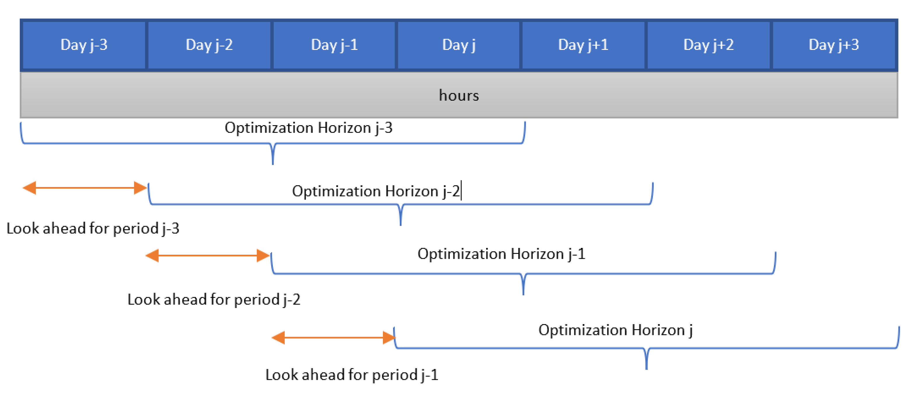
2.2.1. Optimization Horizon

For the present work, the simulation is performed for a whole year with a time step of one hour. In order to improve the computational efficiency, the optimization problem is split into smaller blocks that are run throughout the year as a loop.
An optimization horizon of four days and an overlap period of one day was used to avoid issues linked to the end of the optimization period. Figure 1 shows such an approach. The values of the optimization with which a day is initiated are the final values of the optimization of the previous day. In this case, the optimization is performed over 96 h, but only the first 24 h are conserved [29].

2.2.2. Hydro Scheduling

No midterm scheduling is computed in the model. Thus, all reservoir levels are imposed as historical curves obtained from interpolating monthly time-series; they are delivered as rates of scaled reservoir levels (from 0 to 1). These reservoir levels are set as constraints of the minimum level in the last time interval of the rolling horizon.

2.2.3. Model Formulations, Constraints and Boundaries

The model is formulated as a Mixed Interger Linear Program (MILP) and is solved within the following constraints [29].
  • Energy balance: According to this restriction presented in Equation (2), the sum of all the power produced from all different sources in a node (including storage units generation, imported power from other nodes, and the curtailed power from VRES sources), is equal to the load in that node, plus the power consumed for energy storage, minus the load interrupted and the load shed, for each period and each zone, in the day-ahead market [29].
    u ( Power u , i · Location u , n ) + l ( F l o w l , i · LineNode l , n ) = ( Demand DA , n , h + r StorageInput s , h · Location s , n ShedLoad n , i LostLoadMaxPower n , i + LostLoadMinPower n , i )
  • Power output constraints: If the unit is committed, the minimum power production is defined by the unit’s steady generation level:
    PowerMustRun u , i · Committed u , i Power u , i
    If the unit is committed, the power output is restricted by the available capacity:
    Power u , i ( PowerCapacity u · AvailabilityFactor u , i · ( 1 OutageFactor u , i ) · Committed u , i )
  • Ramping constraints: Each unit has a maximum ramp-up and ramp-down capability. This is translated into limits for ramping up:
    Power u , i Power u , i 1 ( ( Committed u , i StartUp u , i ) · RampUpMaximum u · TimeStep + StartUp u , i · RampStartUpMaximum u · TimeStep ShutDown u , i · PowerMustRu u , i + LLRampUp u , i )
    and limits for ramping down:
    Power u , i 1 Power u , i ( ( Committed u , i ShutDown u , i ) · RampDownMaximum u · TimeStep + ShutDown u , i · RampShutDownMaximum u · TimeStep StartUp u , i · PowerMustRun u , i + LLRampDown u , i )
  • Reserve constraints
    Upward secondary reserve (2U) is the reserve covered by spinning units and is limited by:
    Reserve 2 U u , i ( PowerCapacity u · AvailabilityFactor u , i · ( 1 OutageFactor u , i ) · Committed u , i Power u , i )
    Downward secondary reserve (2D) is similar to the 2U, which is the downward reserve capability of pumping storage units that can only be covered by spinning units and is limited by:
    Reserve 2 D u , i ( Power u , i PowerMustRun u , i · Committed u , i + ( StorageChargingCapacity u · Nunits u StorageInput u , i ) )
    The capability of reserve with quick start (non-spining) is given by:
    Reserve 3 U u , i ( ( Nunits u Committed u , i ) · QuickStartPower u , i · TimeStep )
    The secondary upward and downward reserve demand should be supplied by all the plants authorized in the reserve market:
    Demand 2 U n , h ( u , t ( Reserve 2 U u , i · Technology u , t · Reserve t · Location u , n ) + LL 2 U n , i )
    Demand 2 D n , h ( u , t ( Reserve 2 D u , i · Technology u , t · Reserve t · Location u , n ) + LL 2 D n , i )
    The tertiary reserve can also be provided by non-spinning units with the following constraint:
    Demand 3 U n , h ( u , t [ ( Reserve 2 U u , i + Reserve 3 U u , i ) · Technology u , t · Reserve t · Location u , n ] + LL 3 U n , i )
  • Minimum up/down times: the excessive operation of the generators is limited because of their physical capabilities, there must be a time between starting up and shutting down a generator, and reciprocally vice versa. This constraint for start up is expressed by:
    ii = i TimeUpMinimum u TimeStep i StartUp u , ii Committed u , i
    A similar expression for the minimum down time:
    ii = i TimeDownMinimum u TimeStep i ShutDown u , ii Nunits u Committed u , i
  • Load Shedding: The load shedding is normally regulated and limited by the contracted shedding on that node
    ShedLoad n , i LoadShedding n , i
  • Non-dispatchable units (e.g., wind turbines, runoff-river, etc.): For renewable technologies, the maximum time-dependent generation level is set to directly influence the available factor of the power unit. The outage factor is also taken into account as unavailable power.
  • Multi-nodes with capacity constraints on the lines (congestion) and limited Net Transfer Capacities (NTC) are as follows:
    FlowMinimum l , i Flow l , i Flow l , i FlowMaximum l , i

2.2.4. Mixed Integer Linear Program Solution Process

In the previous paragraphs, we presented the objective function to be optimized; the time horizon was defined and a set of constraints were delivered in mathematical linear inequalities formulated from logic propositions of operational limits of the power system. The Unit Commitment (UC) aims to find a low-cost operating schedule for the power-generator units optimizing the objective function within its constraints. In this sense, power systems are typically large and mixed, integer non-linear and with non-convex operation constraints, with quadratic objective functions. In the present work, the UC formulation is linearized using the LaGrange relaxation in order to solve the UC optimization problem with discrete programming. Thus, the method applied for finding optimal solutions of various optimization problems is the branch-and-bound algorithm. It consists of discrete and combinatorial optimization with a systematic enumeration of all candidate solutions, where large subsets of ineffective candidates are identified by using upper and lower estimated bounds of the quantity being optimized. The theory and algorithms of the discrete optimization solution can be found in detail in [14,32,33,34].

2.3. Input Data

The model is data-intensive and requires high technological, temporal and geographical granularity inputs such as a power plant database (non-variable in time), consumption and generation time-series, grid topology, etc. The main model inputs are described in the next sections.

2.3.1. Power Plant Database

The power plant database has specific fields of techno-economic information of every power plant operating in the power system by default. They are briefly listed and presented in Table 1. Their values are preferentially obtained from the system operator. When not available, reference values are taken from relevant references.
For thermal units, ramping costs and startup costs become crucial since the on/off rate of these units and ramping changes are increased in response to a fluctuating system (load or supply) requirement due to VRES penetration.
Prices of fuel and fuel type are important to collect; they can be found in [35,43,44]. The international prices at which Bolivia exports natural gas and gas oil are are 10.42 EUR/MWh and 17.19 EUR/MWh, respectively. However, in Bolivia, the prices of natural gas and gas oil are subsidized by the government. The subsidized prices are 3.57 and 13.91 EUR/MWh, respectively [35,43,44]. For the present work, we suggest using only the subsidized prices to focus only in the technical effects of VRES high penetration. Moreover, Sugarcane pellets prices are taken as 0 EUR/MWh since the bagasse of residual cane from the Bolivian sugar industry was used. Considering that the present Bolivian regulation lacks a CO 2 pricing scheme, a CO 2 emission input does not affect the results. We therefore assume costs related to CO 2 emissions at zero.

2.3.2. Time-Series Data

Time-series data are historical data for the time period analyzed and are composed of 8784 or 8760 data points for each time series. The methodology of data acquisition and determination of time series is described in the next subsections. In some cases, we interpolate monthly data available to generate hourly time series. Reference data available in the bibliography are assumed when the information is restricted by national entities.
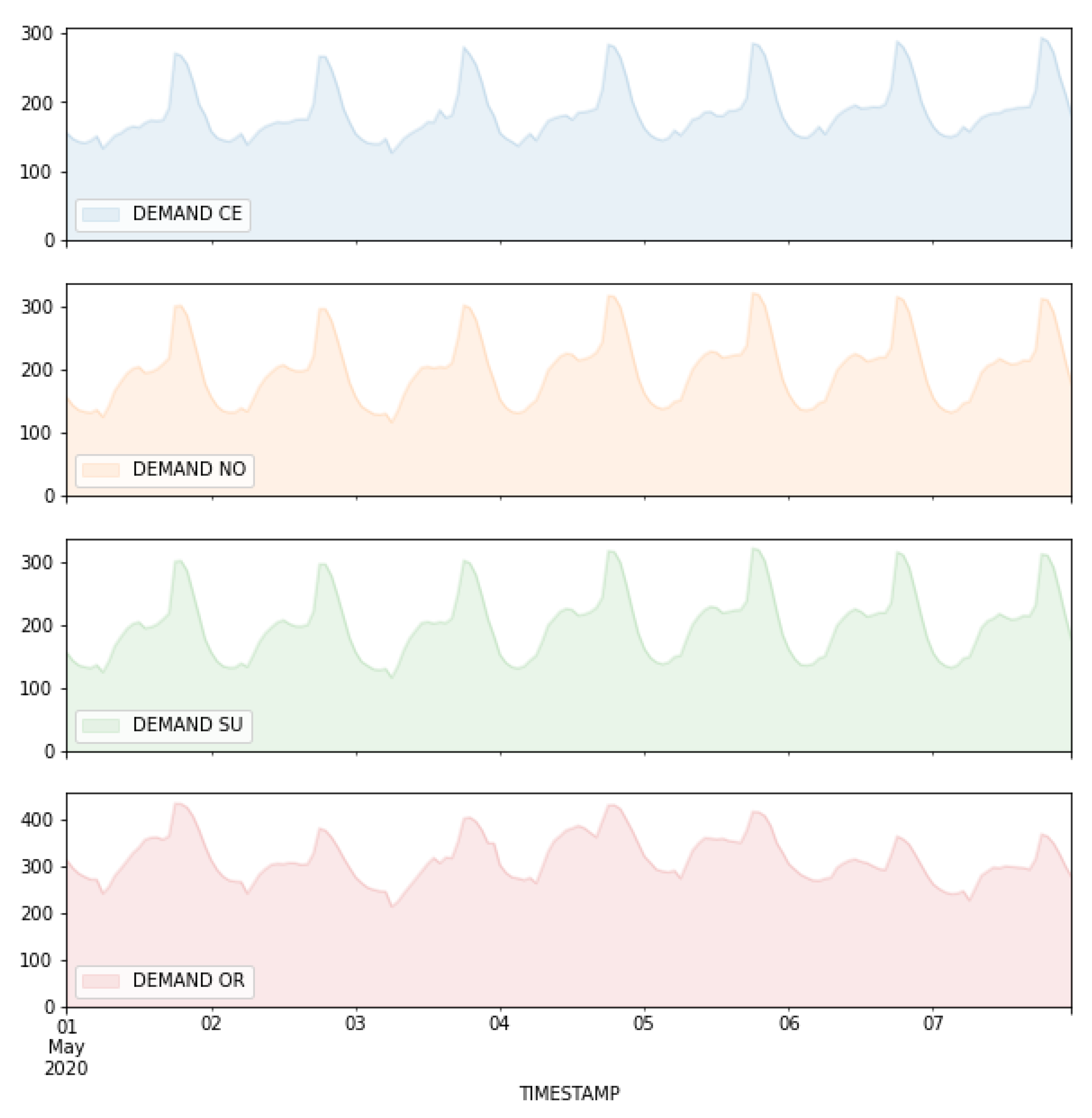
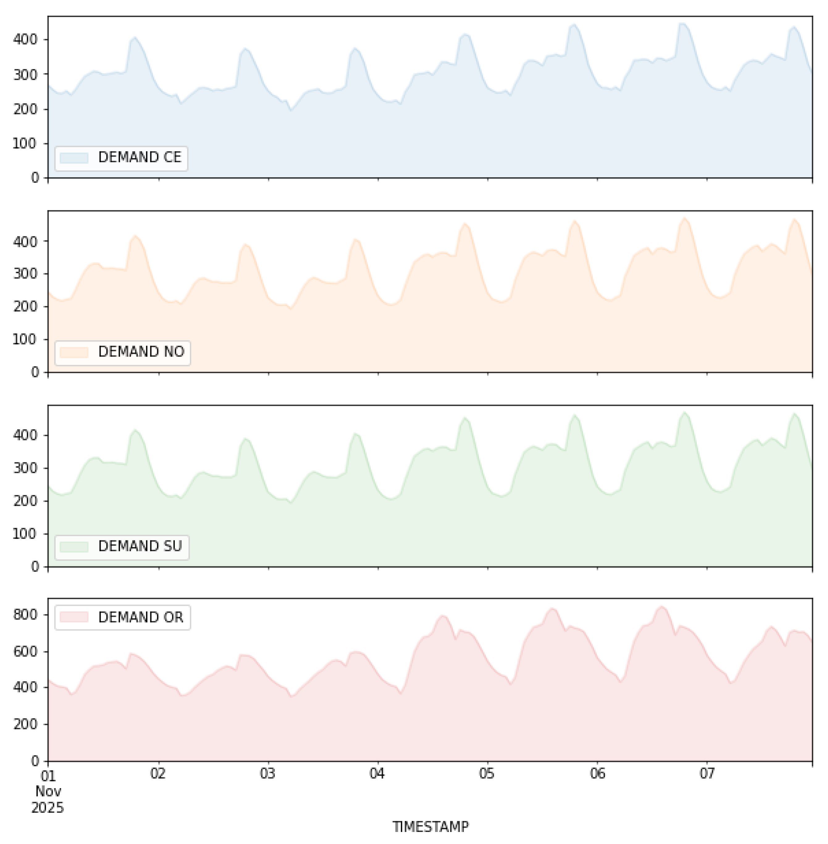
  • Times series related to the energy demand in each node of energy consumption: central, north, oriental and south zone. The baseline time series are obtained from the national system operator (e.g., CNDC [45]). However, this demand cannot be considered constant in time. A percentage factor of demand growth is therefore assumed for future scenarios.
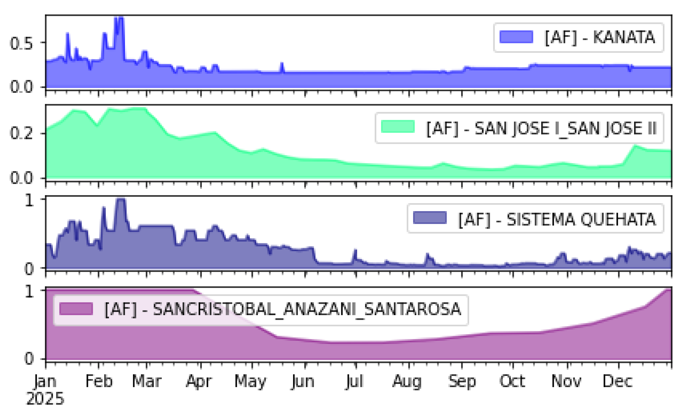
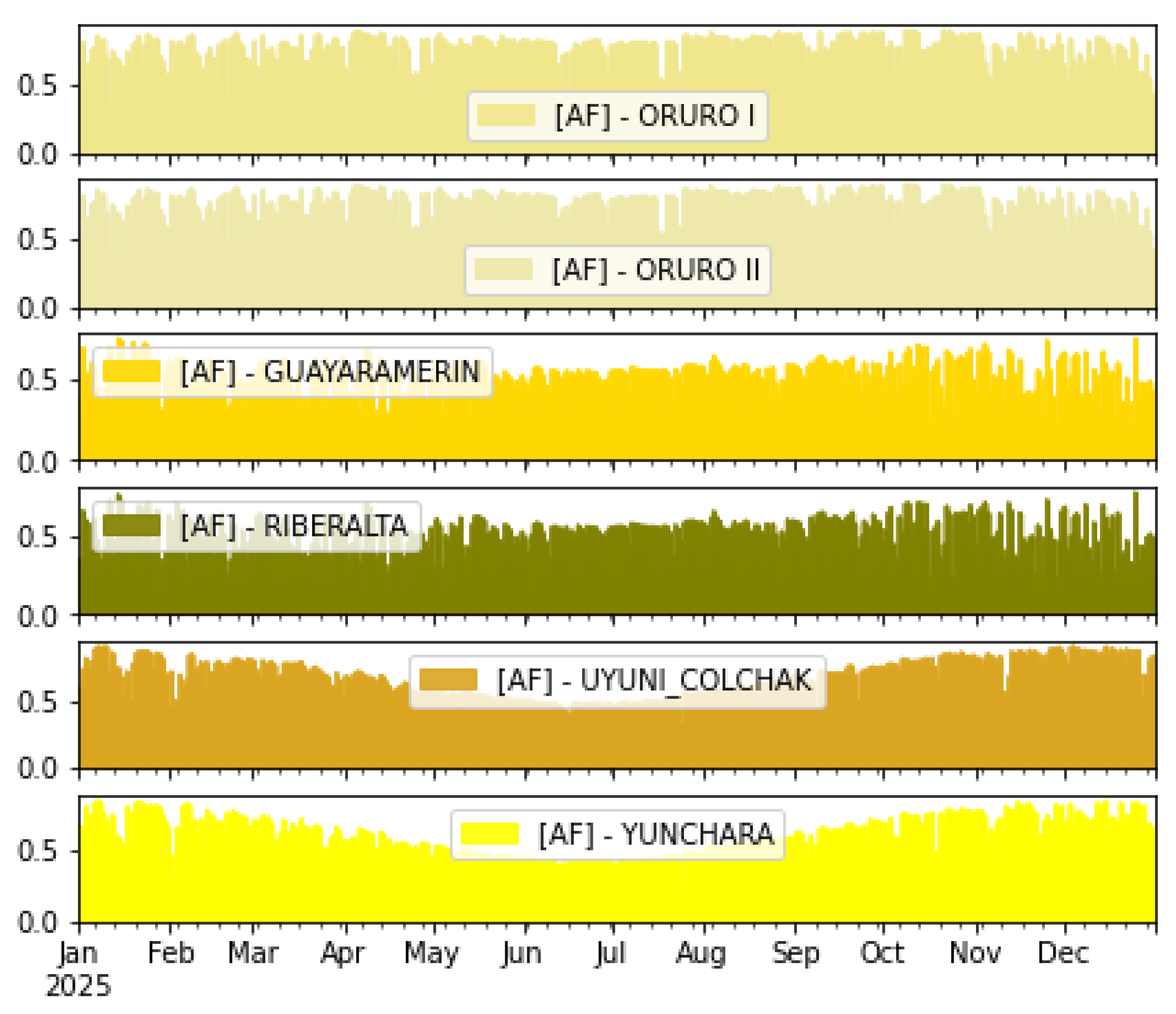
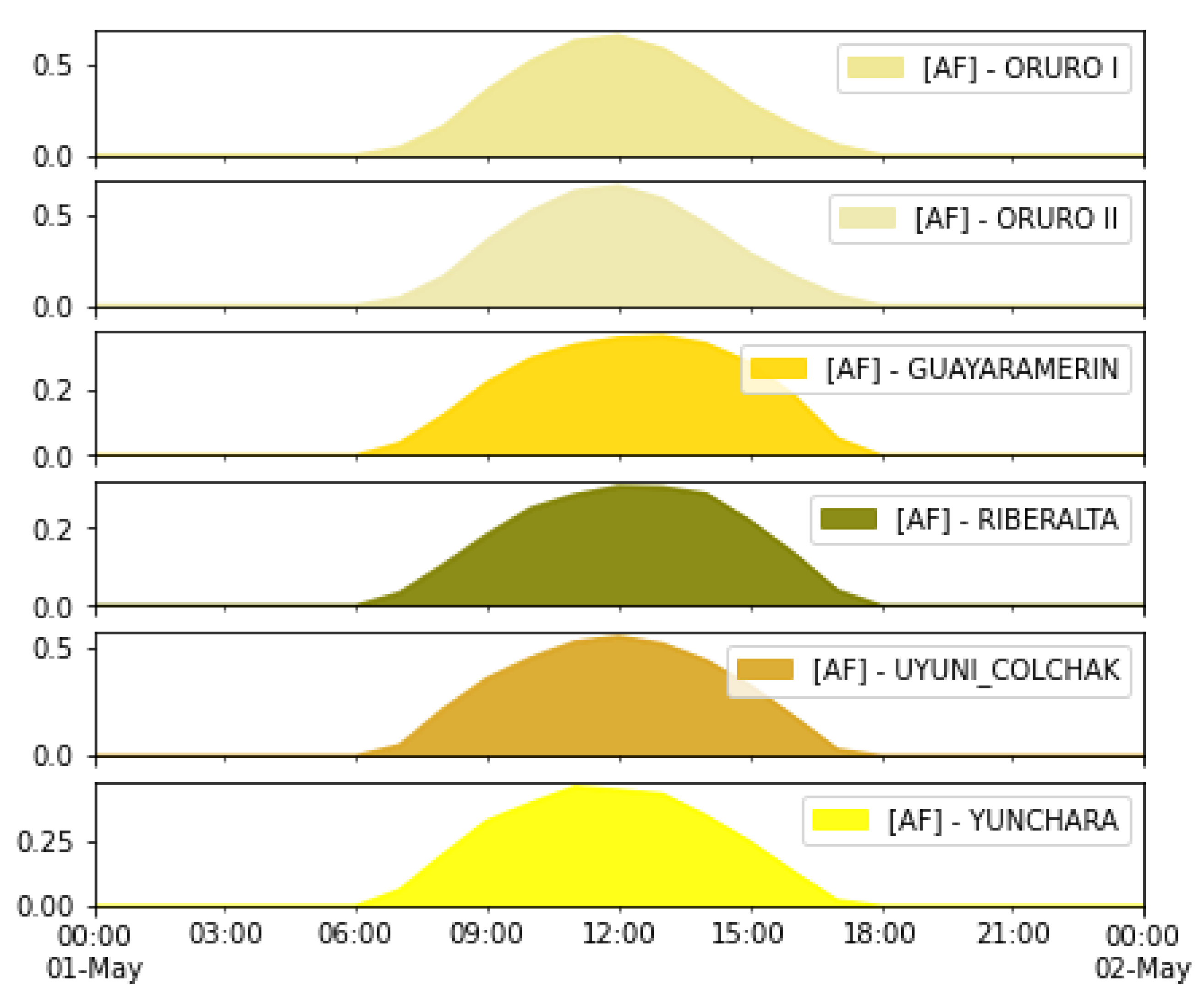
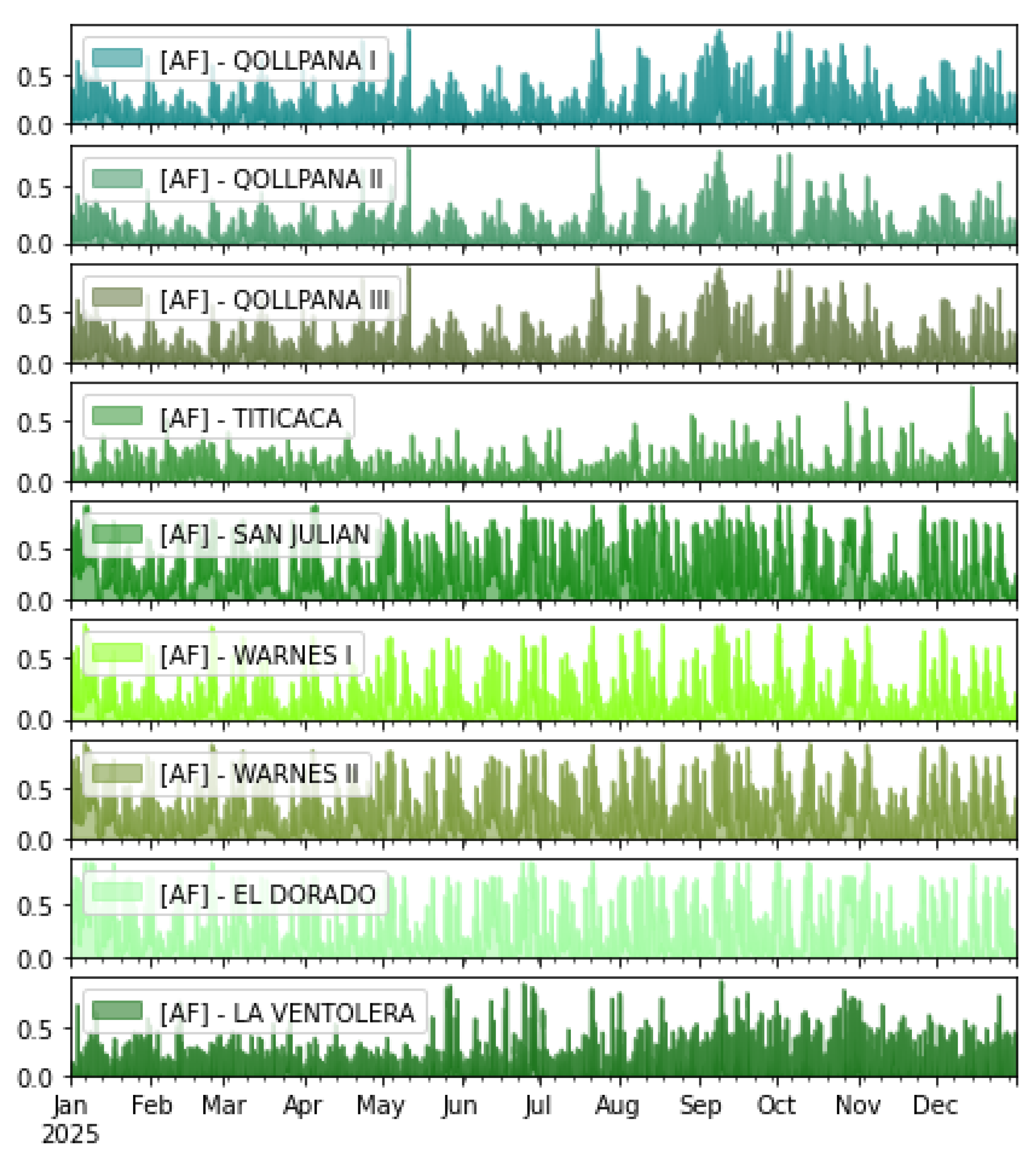
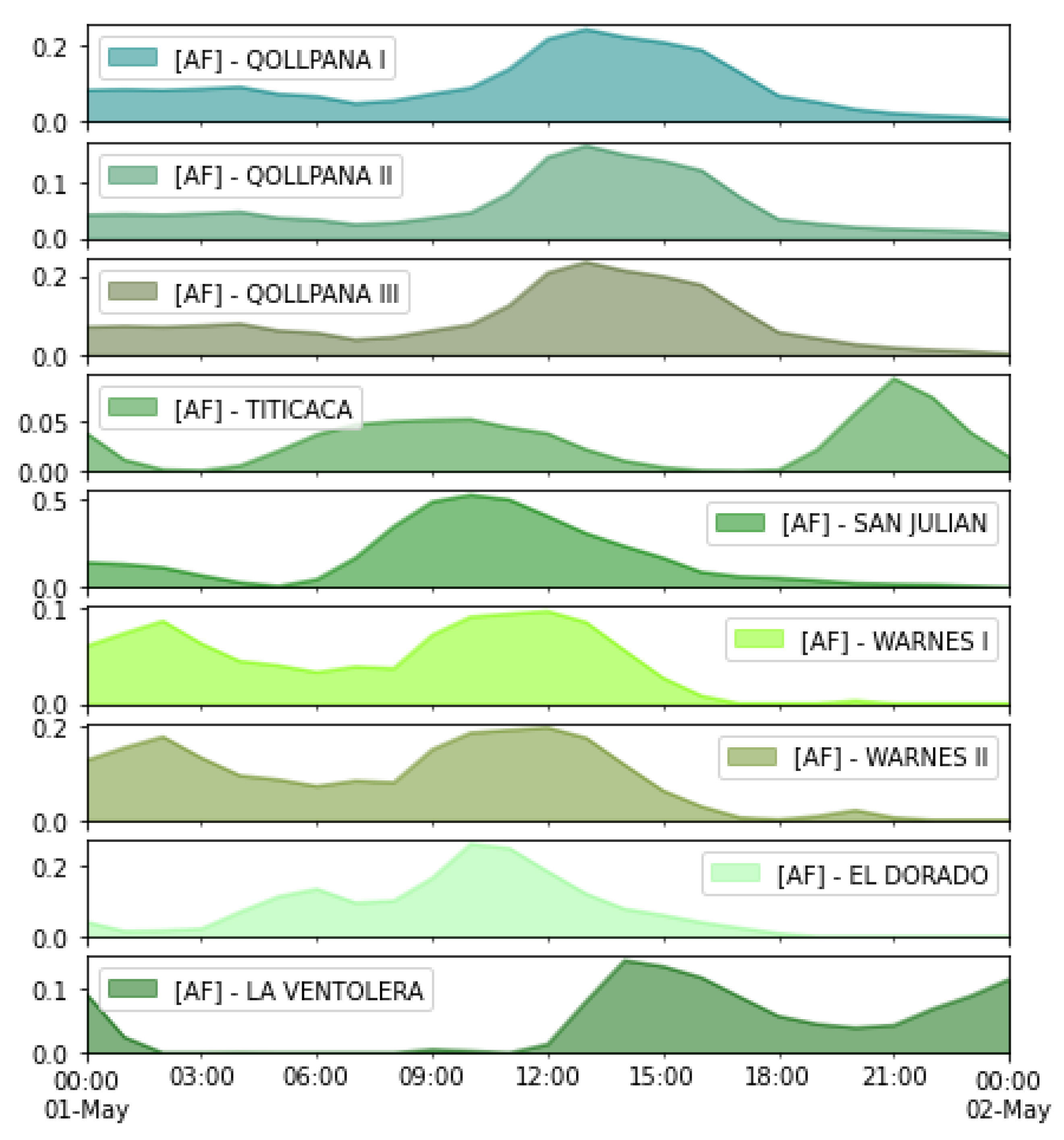
  • Availability Factor: VRES technologies include HROR (run-of-the-river hydro), WTON (onshore wind) and PHOT (photovoltaic solar). Their generation is defined as a proportion of the nominal power capacity, referred to as “availability factor”, and is provided as an hourly time series [29].
  • Scaled inflows are expressed as a fraction of the nominal power of each unit with hydro storage, and they are provided externally as an hourly time series [29]. They are gathered from [46].
  • Storage levels are individual time series corresponding to historical volumes accumulated in each reservoir of the SIN. They are imposed as a lower boundary when each optimization horizon ends. Their mathematical expression is as a fraction of maximum storeable energy [29]. Weekly storage-level averages can be found in [47], from which we generated hourly time series.

2.3.3. Grid Data

Interconnections are modeled through their net transfer capacities (NTCs). They correspond to the commercial transfer capacity between the nodes considered in the simulation. A review of the characteristics of the main interconnection lines in the Bolivian case is available at [42].

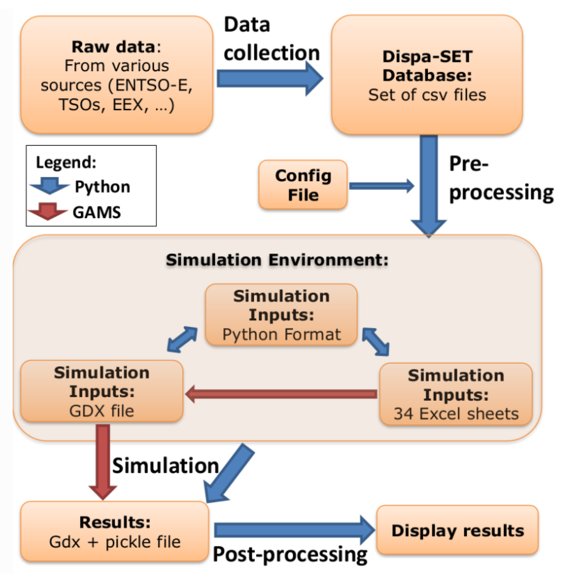
2.4. Model Implementation

These input data are gathered in the pre-defined and imposed Dispa-SET format. In the following paragraph, we present the objective function of the model and its current features. However, the detailed unit commitment problem and implementation of the model can be found in [29]. Figure 2 describes the implementation and the work flow of the model. The results allow us to analyze and evaluate the techno-economic incidence, correlation and restrictions of the different variables in the database for mid-term and long-term time horizon scenarios. They also allow us to quantify the system flexibility against the variability of the VRES. This last feature is deductible in terms of curtailment, load shedding and storage levels.

3. The Bolivian Case Study

The Bolivian Power System (SIN) shows a growing interest from the Bolivian authorities to integrate more renewable energy sources. This is evidenced, e.g., in the SIN expansion plan (PEEBOL2025, Plan Eléctrico del Estado Plurinacional de Bolivia 2025 [42]) and in the annual reports of the different subsidiaries of the National Energy Company (Empresa Nacional de Electricidad, ENDE). In these documents, multiple feasibility and pre-feasibility studies are listed for several run-of-river hydroelectric plants up to 2025 and beyond [42,48]. However, these expansion plans currently only involve a limited number of wind, solar or geothermal plants. Although PEEBOL2025 has been implemented since 2014, the Bolivian electric power matrix is changing slowly compared to other countries in the region (Uruguay, Brazil, Argentina, Chile). The production of VRES increased in percentage from 1.5% (120 GWh) in 2014 to 11% (1046 GWh) in 2020 of the total supply in each year [49,50]. As a result of this slow penetration rate of VRES, the country still depends on natural gas as a primary energy source [25].

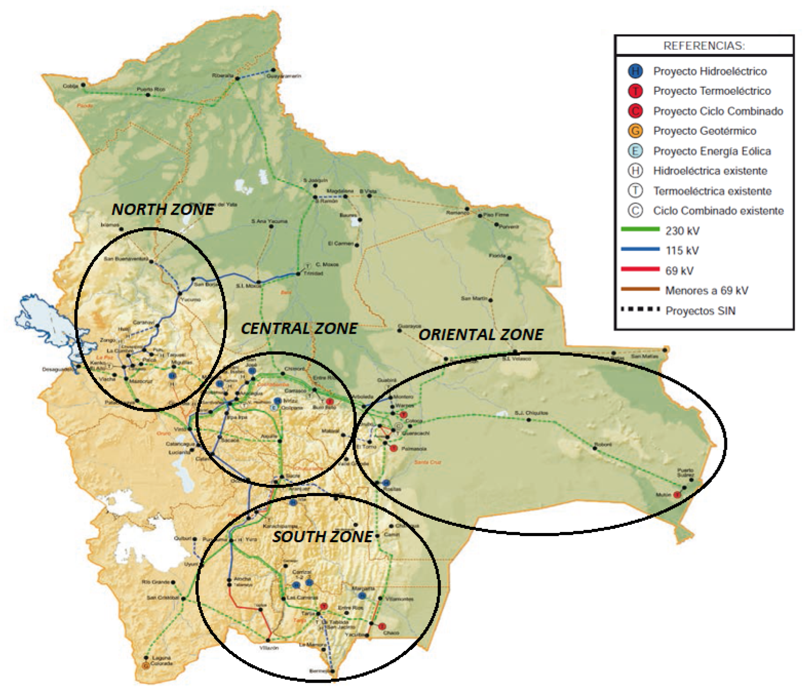
3.1. Power System Topology

In Bolivia, the power system is radial and is arranged by areas defined almost naturally by its geography. La Paz and Beni constitutes the North. Santa Cruz and Pando shape the Oriental zone. Oruro and Cochabamba comprise the Central zone. Finally Potosí, Chuquisaca and Tarija in the South zone. Figure 3 shows this zones placed and marked in the map of Bolivia.
The transmission system is composed of transmission lines with high levels of voltage: 69 kV, 115 kV and 230 kV. This transmission lines shape the main power system grid known as STI (Sistema Troncal Interconectado).
The power generation is provided by power units with the following different technologies and fuels:
  • Hydroelectric run-of-river power units (HROR WAT),
  • Hydroelectric power units with dams (HDAM WAT).
  • Open-cycle natural power units (GTUR GAS),
  • Combined cycle power units (COMC GAS).
  • Diesel engines (GTUR OIL).
  • Biodiesel power units (GTUR BIO).
  • Wind-onshore turbines (WTON WIN).
  • Finally, there are two PV solar power plants (PHOT SUN).

3.2. Energy Demand for 2025

The energy demand of Bolivia is mostly residential. The demand is divided into two categories: regulated consumers supplied by distribution companies and non-regulated that directly participate in electricity markets [35]. By 2020, the energy demand is higher in the Oriental zone at 38.5%, next is the North zone with 23.39%, followed by the Central zone with 22.36% and finally the South zone with 15.69% [35]. The energy demand increased from 8378 GWh in 2016 to 9212 GWh in 2020. For the following years, the projection of the demand was based on large consumer statements, bottom-up methods, methods based on interpolation of growth rates and methods based on the evolution of specific consumption by categories of distributors. A growth rate at an average of 4% per year was determined, reaching a demand of 12,310 GWh for the year 2025 [42].
The time resolution of the energy demand time series is hourly for a period of one year.The energy demand for the year 2020 was extracted from [45] and is provided individually for each zone of the power system mentioned before. Figure 4 and Figure 5 show examples of load curves for the four zones comprising the power system. The load time series for the year 2025 is determined by applying a yearly growth rate to the 2020 load time series, identified from [42].

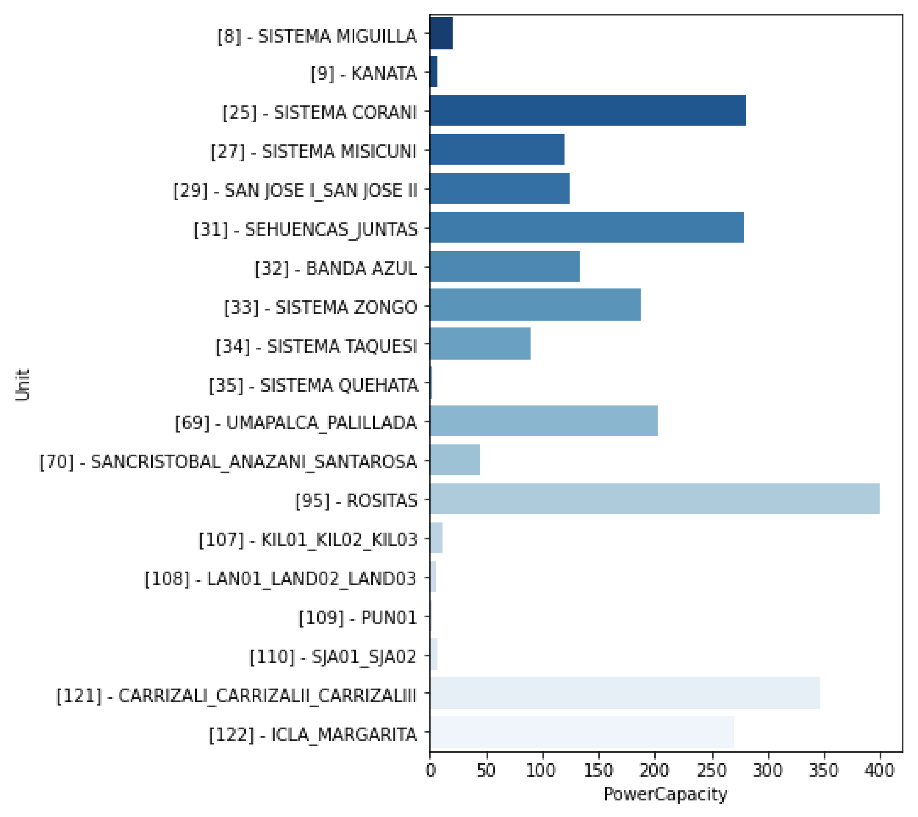
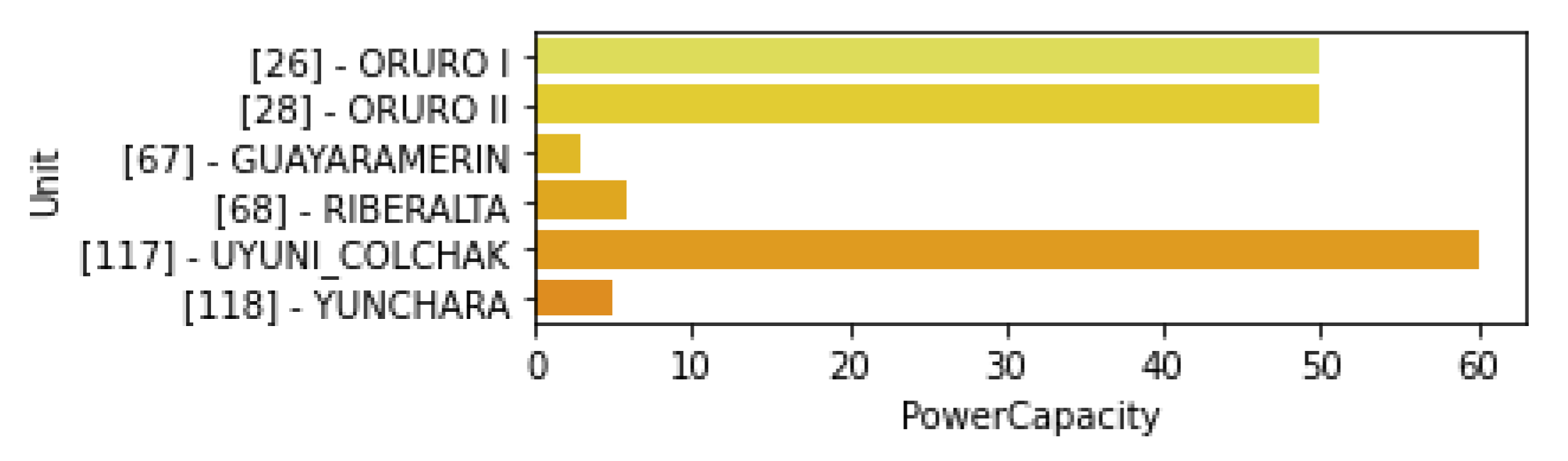
3.3. Power Plants Fleet for 2025

The SIN generation’s installed effective capacity until 2020 is presented in Table 2, disaggregated by zones and technologies. There is a strong reliance on conventional power generation technologies (thermal and hydroelectric) with a reduced supply from wind, solar and geothermal generation. It reaches a total capacity of 3187 MW, of which 859 MW (26.95%) corresponds to hydroelectric plants. Thermal generation still represents the main primary energy source with 2186 MW (67.18%), 27 MW (0.85%) corresponding to wind farms, 115 MW (3.61%) to solar energy and finally 45.22 MW (1.41%) to biomass power plants.
Based on energy policies and demand requirements, PEEBOL2025 proposes a portfolio of generation and transmission projects until 2025 for the expansion of the electrical infrastructure considering the availability of energy sources. According to [35], the total electricity consumption in 2025 is expected to reach 12.31 TWh, and the generation capacities will be increased: the total installed capacity will exceed 5.19 GW, from which 2.14 GW (41.23%) will be thermal, 2.54 GW (48.85%) will be hydroelectric, 0.22 GW (4.28%) will be wind-onshore, 0.17 GW (3.35%) will be solar PV and 0.45 GW (0.87%). PEEBOL2025 data reveal that the following five years (2020–2025) the SIN expansion plan will integrate VRES projects in an average of 50MW per year [35]. A summary of planned generation projects in each zone is provided in Table 3 [35,42,48,51,52].

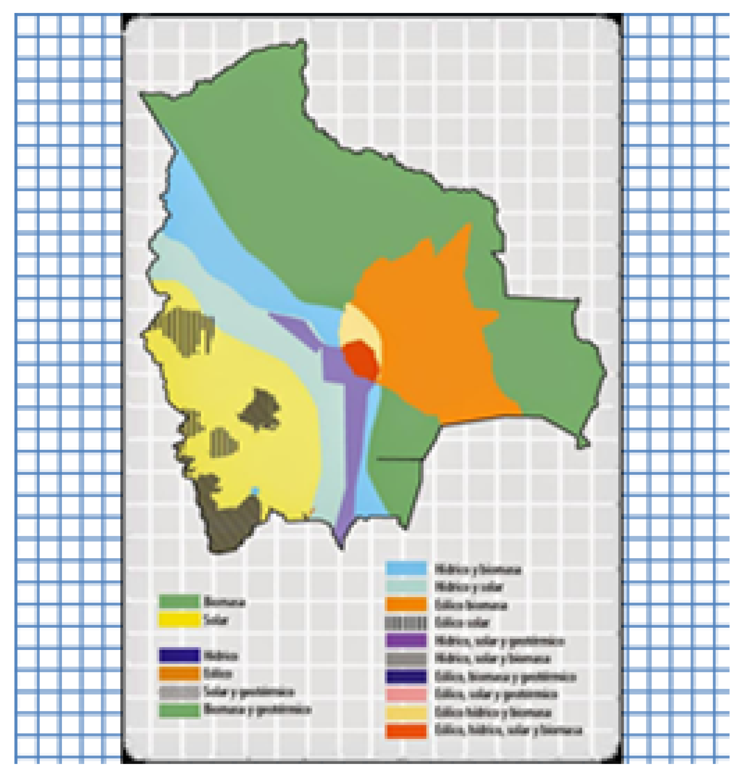
3.4. VRES Generation Capacity for 2025

The VRES potential in Bolivia is distributed throughout the territory. Hydro-run-of-river (HROR) projects are found in all four zones of the SIN; however, the main HROR projects are located in the central and south areas. Solar energy is feasible in all regions but is particularly suitable for the Andean highlands sector due to its high levels of radiation. Finally, in the departments of Cochabamba and Santa Cruz and in some highland areas nearby, wind energy is predominant [23]. Despite the VRES expansion potential shown in Figure 6, Figure 7, Figure 8 and Figure 9, the projects planned until 2025 only represent 9.24% of the total effective capacity by that year.

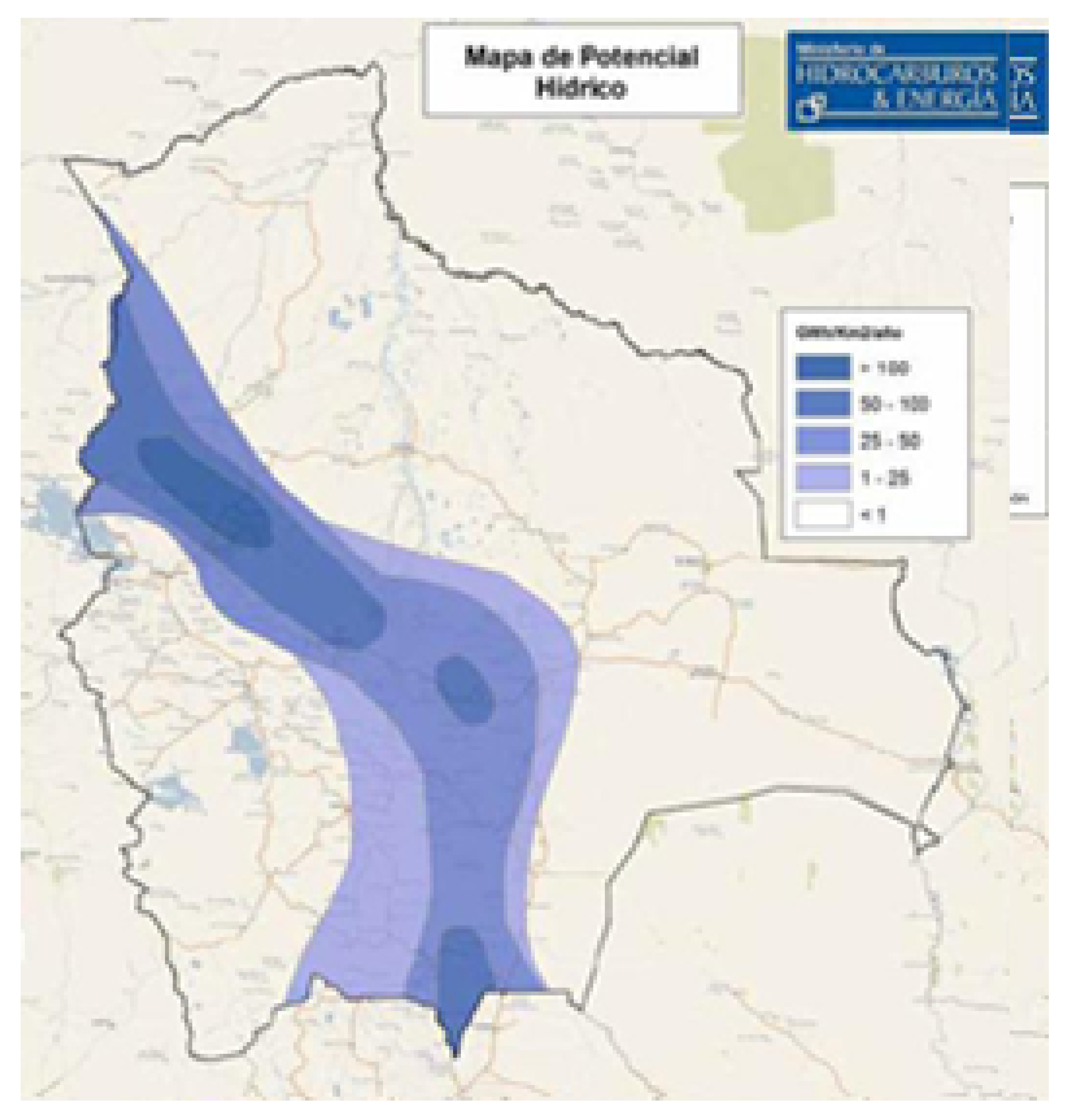
3.4.1. Hydro Resources

The hydroelectric projects were chosen from the studies carried out in different stages of pre-investment and/or pre-feasibility studies [52]. They are located in different regions of Bolivia. Two important projects were completed and started operations in 2020: Misicuni with 120 MW, and San José with 120 MW, as the third stage of the use of the waterfall in the upper basin of the Chapare River.
The hydroelectric generation project portfolio for 2025 includes the incorporation of Miguillas with Umapalca (83 MW) and Palillada (113 MW) hydroelectric plants, located in the department of La Paz, Ivirizu (164 MW) in the department of Cochabamba, Rositas (400 MW) in the department of Santa Cruz on the Rio Grande river, Icla (102 MW) in the departments of Chuquisaca and Potosí on the Pilcomayo river, the Carrizal I, II and III Project (347 MW) on the Camblaya river located between the departments of Tarija and Chuquisaca, and Margarita (150 MW), located in the “Chaco Tarijeño” on the Pilcomayo river. These projects (Figure 10) will contribute to the change of the energy mix with a notable increase of the system inertia and the spinning reserve and will supply the country growing energy demand with 1599 MW [42].
Availability factors for hydro run-of-river resources are derived from interpolating average weekly flows obtained from [46]. Unit technical data such as turbine type, efficiency, nominal power and height of fall were gathered from [54]. Every run-of-river unit is assigned with its own availability factor distribution expressed in time series (e.g., Figure 11).

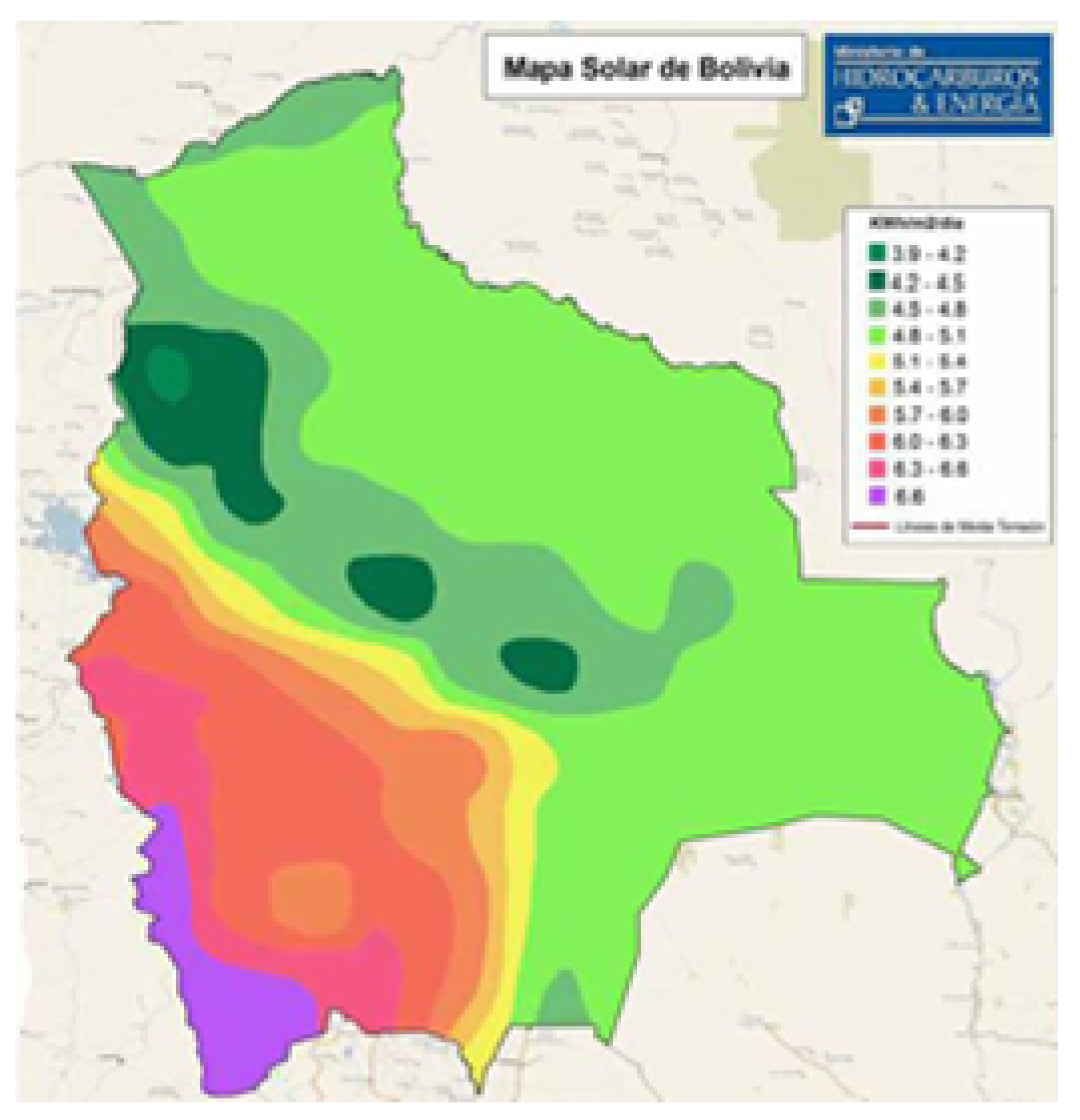
3.4.2. Solar Resources

The southwest region of the country, as shown in Figure 7, has the highest radiation rates (5.1–7.2 kWh/m 2 -day), whereas the northeastern region has the lowest rates (3.9–5.1 kWh/m 2 -day) [55,56]. Because sunrise and sunset hours vary by only one hour throughout the year [57], the radiation rate does not exceed 25% between the winter and summer seasons [58]. Additionally, due to Bolivia’s high altitude above sea level, the dry climate produces a lower solar dispersion, and thus a large part of the country is subjected to the world’s highest level of solar radiation (the tropical zone of the south between parallels 11° and 22°) [58]. Over 97% of the country’s territory is suitable for using solar energy as a primary energy source [59]. In contrast, PEEBOL2025 does not mention large-scale solar-energy-integration projects. In 2020, the SIN incorporated its three first solar energy projects: Oruro I (50 MW), Uyuni ColchaK (60 MW) and Yunchara (5 MW). Additionally, at least three more projects are confirmed to be completed by 2025: Oruro II (50 MW), Guayaramerin (3 MW) and Riberalta (5.8 MW) with a total installed solar energy capacity of 173.8 MW until 2025. In Figure 12, the solar plants are presented with its respective power capacity.
By providing the approximate geographic locations [60] of the solar power plants, it was possible to generate time series of solar availability factors and monthly average solar radiation data of Bolivia using radiation models. For the present work, we used [61]. Additionally, the environmental features [62,63] and PV systems technical features [64,65,66] are useful to validate the information generated with the radiation models. (e.g., Figure 13 and Figure 14).

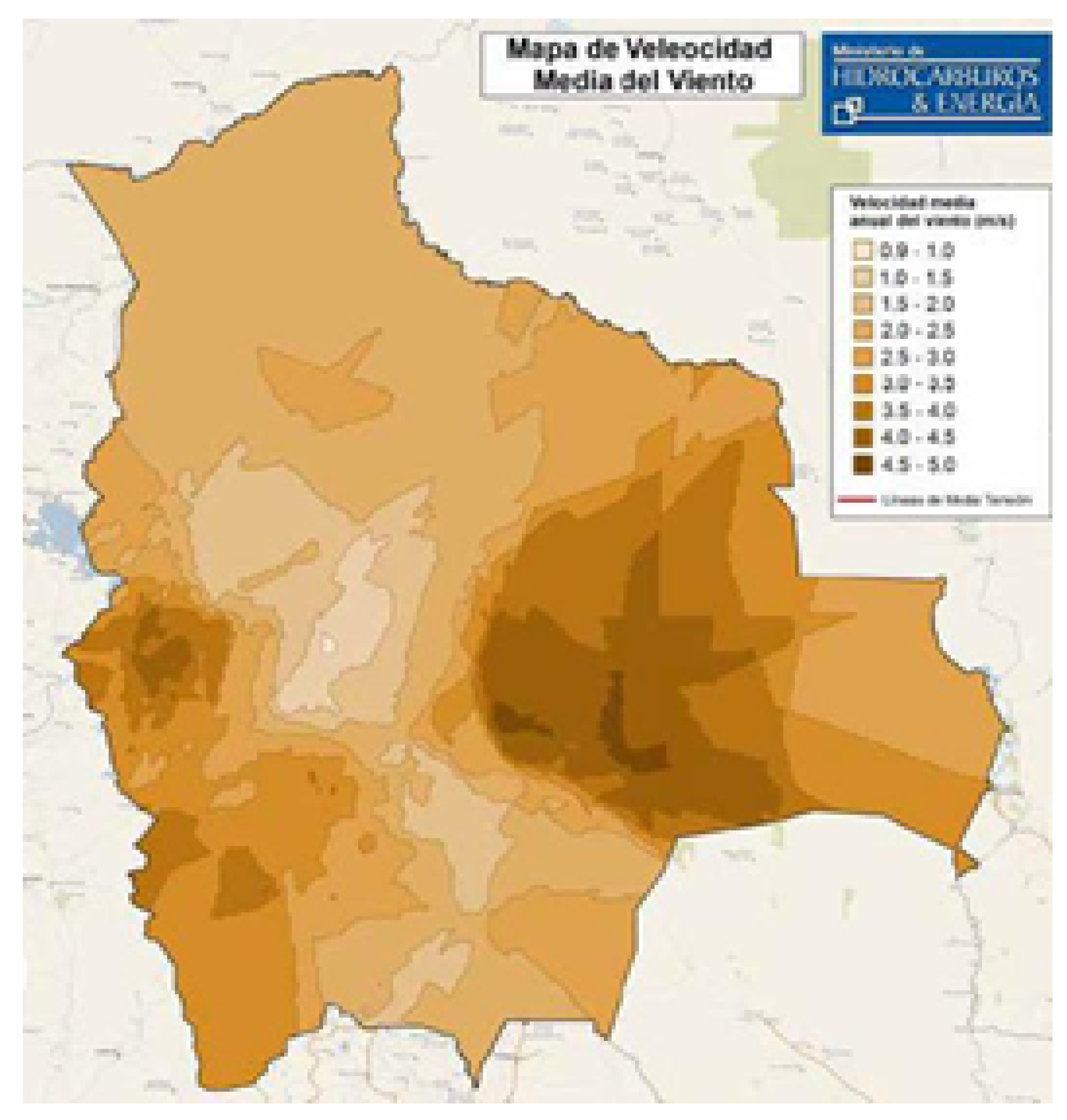
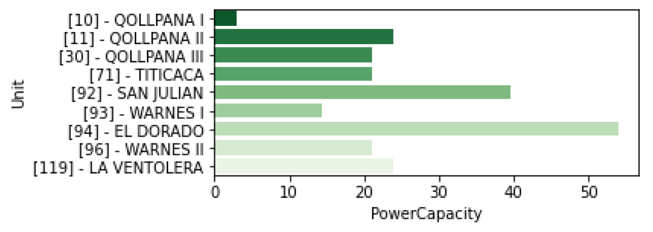
3.4.3. Wind Resources

Wind generation is evaluated based on the Bolivian wind atlas [67] and wind speed measurements at three different heights for a whole year (20 m, 50 m, 80 m). Wind resources in Bolivia are more limited than solar, as indicated in Figure 8. Stronger resource are concentrated in five sectors, and the first wind farm projects are incorporated gradually: on the South and Sest of Santa Cruz city, mostly, with the projects “Warnes-El Dorado" and "San Julian”; from La Paz to Santa Cruz, north of Cochabamba, on the corridor that goes fro, east to west with the project “Qollpana I-Qollpana II-Qollpana III”; on the corridor between Tarija and Sucre departments, which goes from north to south with the project La Ventolera”; around the Titicaca Lake region in the department of La Paz with the project o “Titicaca”; and finally, at the southwest border between Chile, Argentina and Potosi department. The area on the north-to-south corridor between Oruro and Potosi departments provides possible locations for future projects [67]. In Figure 15, the wind power plants are presented with their respective power capacities.
Wind resource availability factors are generated based on wind speed data from [61] and the approximate geographic location and technical characteristics of both installed and planned wind turbines from [68,69,70] (e.g., Figure 16 and Figure 17).

3.5. Grid Data for 2025

The Bolivian grid is relatively simple and radial. There are only four zones clearly defined in the country. Energy can be exchanged between these zones by way of transmission lines, whose power flows are limited by net transfer capacity (DC power flow is not implemented in the current model). Table 4 summarizes the maximum capacity of each transmission line that interconnects the four zones, installed by 2020, extracted from [35].
Based on [35], grid data were also upgraded up to the year 2025, by which a 160 MW line will be added between North and Oriental, a 100 MW line will be added between Central and North, a 300 MW line will be added between Oriental and South, and a 300 MW line will be added between Central and South. Table 5 summarizes the planned transmission projects between the four regions. It is noteworthy that the government is considering interconnection projects (called mega-projects), which are geared toward energy exchange with neighboring countries. Nevertheless, the schedule has not yet been announced and these projects are therefore not considered in this work [52]. In this context, the Bolivian power system is considered an isolated case of study.

3.6. What-If Scenarios

The baseline scenario of the Bolivian interconnected power system (SIN) by 2025 was built from the known information relative to the SIN of the last year 2020 and assembled, adding to the information of that year all the projects listed in the PEEBOL 2025 (Electrical Plan of the Plurinational State of Bolivia–2025). It was built as a simplified representation of the power system, gathering all the technical information and operative policies from the official web page of National Power dispatch Committee (CNDC, operator of the SIN) [42] and annual records of the ENDE corporation [48,51,71]. Building upon this baseline, multiple determined what-if scenarios were formulated:
  • Low-penetration scenarios 1 and 2, with 402 MW and 670 MW of VRES installed capacities, respectively.
  • Moderate-penetration scenarios 3 to 5, with 938 MW, 1072 MW and 1206 MW of VRES installed capacities, respectively.
  • High-penetration scenarios 6 to 8, with 1340 MW, 2342 MW and 5142 MW of VRES installed capacities, respectively.
  • Finally, Very-High-penetration scenarios 9 and 10: with 7642 MW, 10,142 MW and 804 MW of VRES installed capacity.
For each penetration scenario, the reservoir capacity of the hydro dam is assumed to be fully exploited (H scenarios) or completely discarded (NH scenarios). This is used to evaluate the potential contribution of the hydro sector to balance the variations of VRES.
All the parameters summarized in Table 6 were set and implemented into the model as input data to create the simulation environments (in separate folders) for each scenario described before. These variations of input parameters are a batch of simulations of the unit-commitment and optimal dispatch (UC/D) model. Finally, the results allow the possible impact of a large deployment VRES generation to be understood with and without HYDRO storage. The simulations were developed in terms of energy balance, transmission grid capacity, system reserves capacity translated in system inertia, ancillary services requirement and energy generation cost. It should be noted that the installed power capacities of other technologies were kept unchanged, and the current locations of VRES units were conserved.

4. Results and Discussion

The results of the different scenarios are summarized in Table 7, Table 8 and Table 9 and Figure 18, Figure 19, Figure 20, Figure 21, Figure 22, Figure 23, Figure 24, Figure 25, Figure 26, Figure 27, Figure 28, Figure 29, Figure 30, Figure 31, Figure 32 and Figure 33. In the following subsections, the most relevant simulation outcomes for all scenarios are discussed.

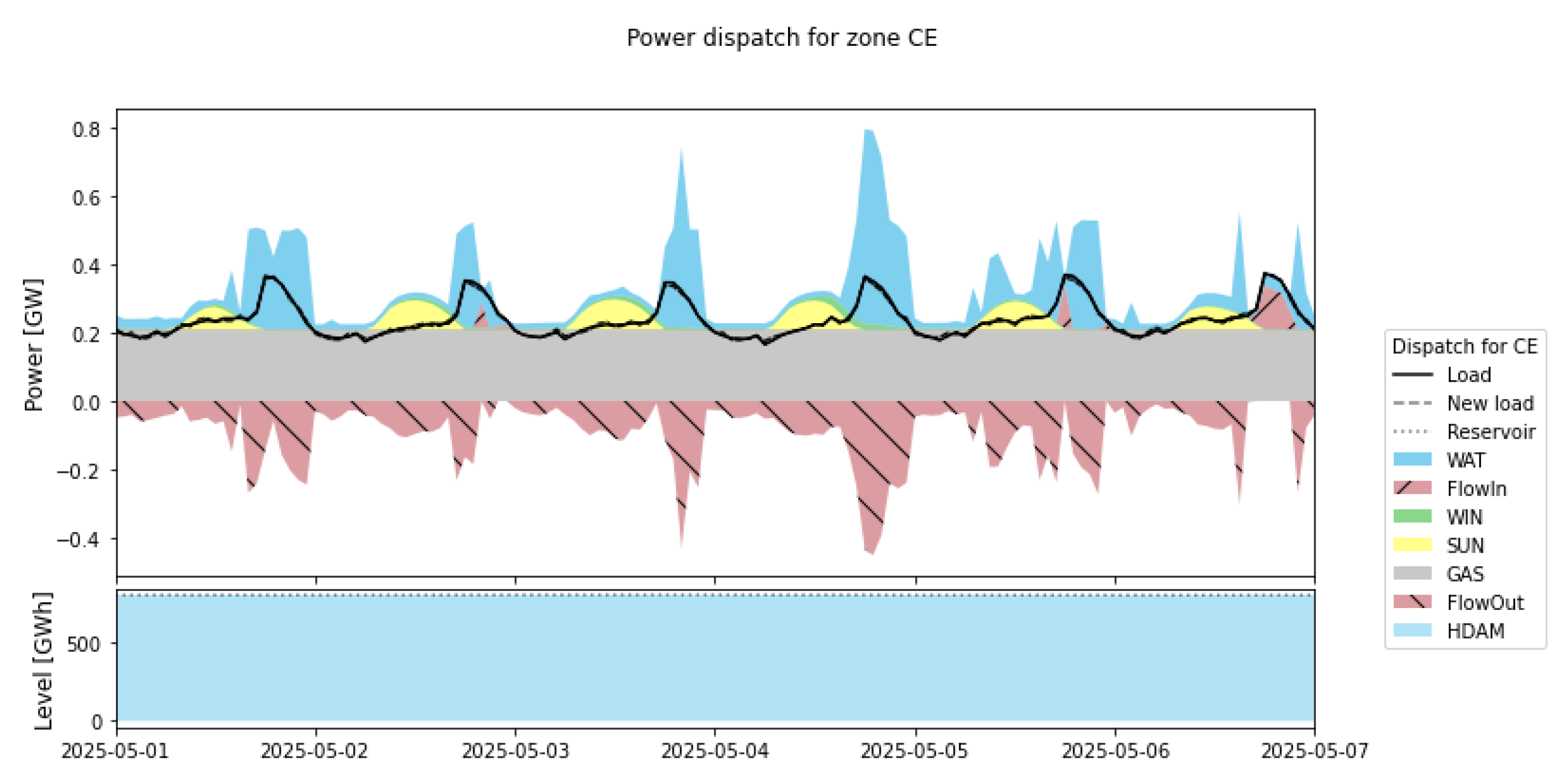
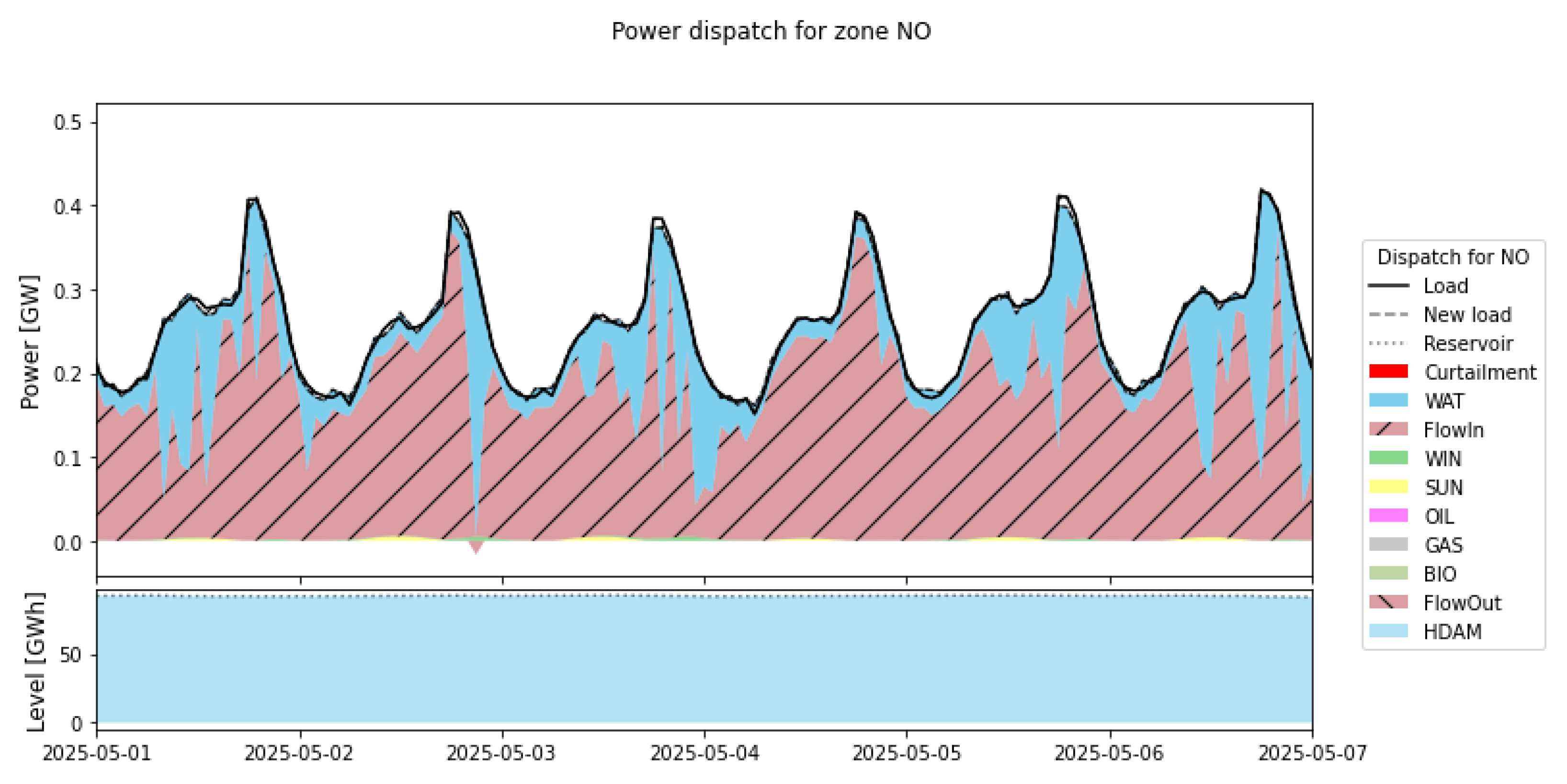
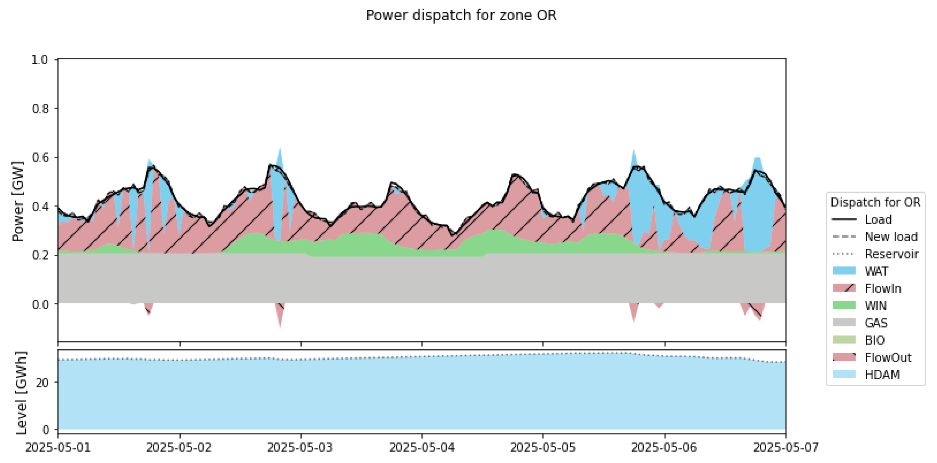
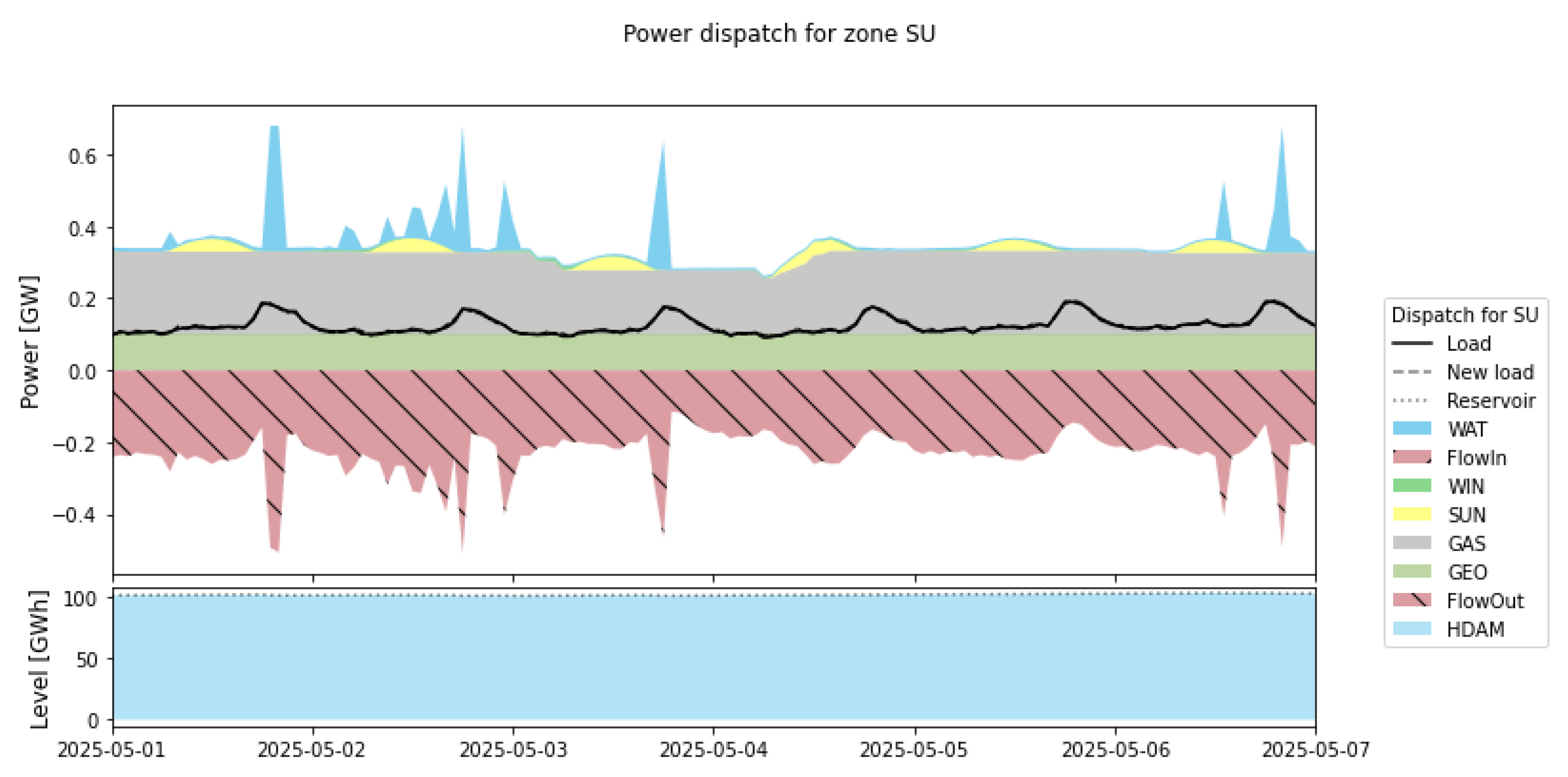
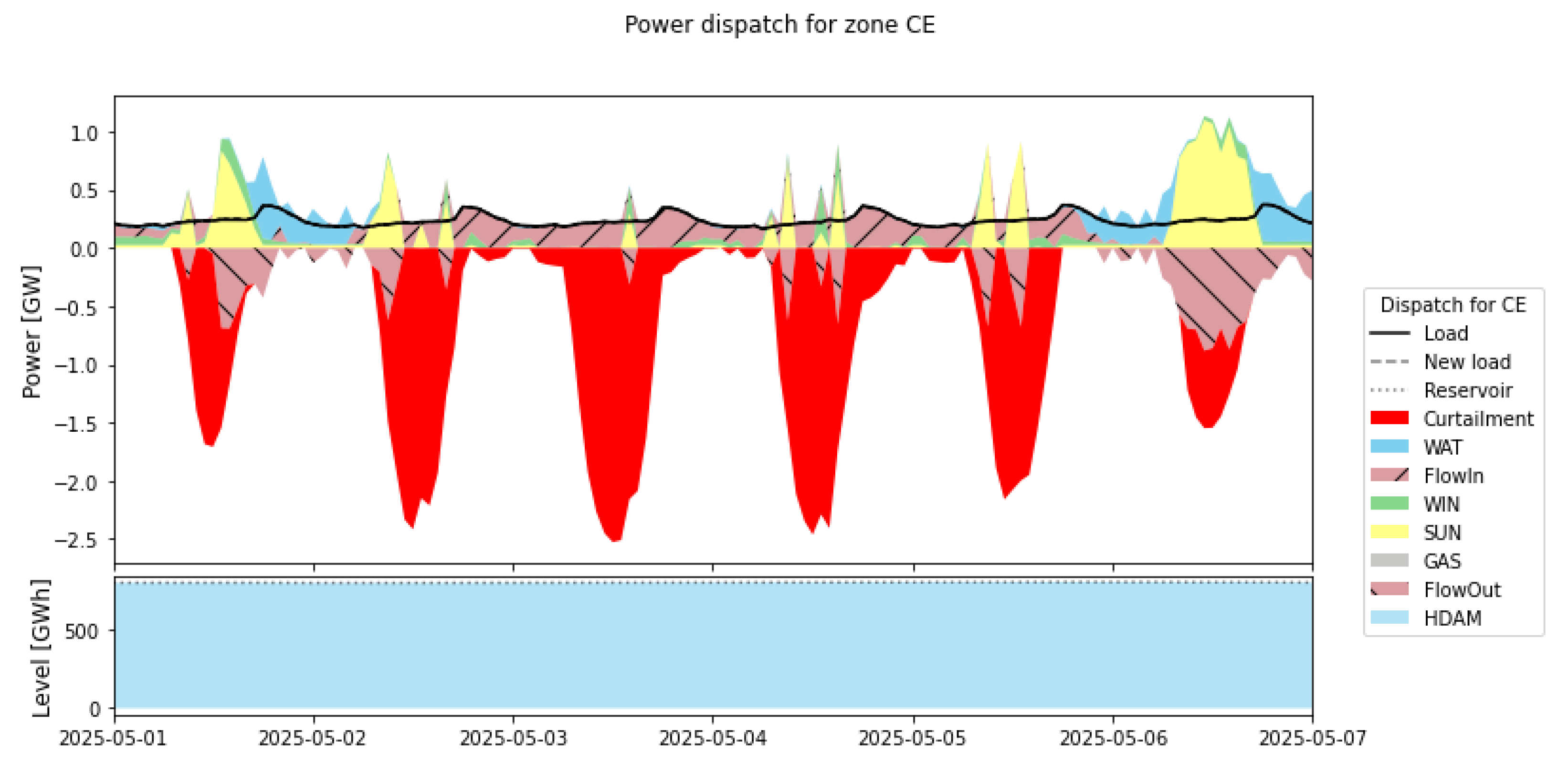
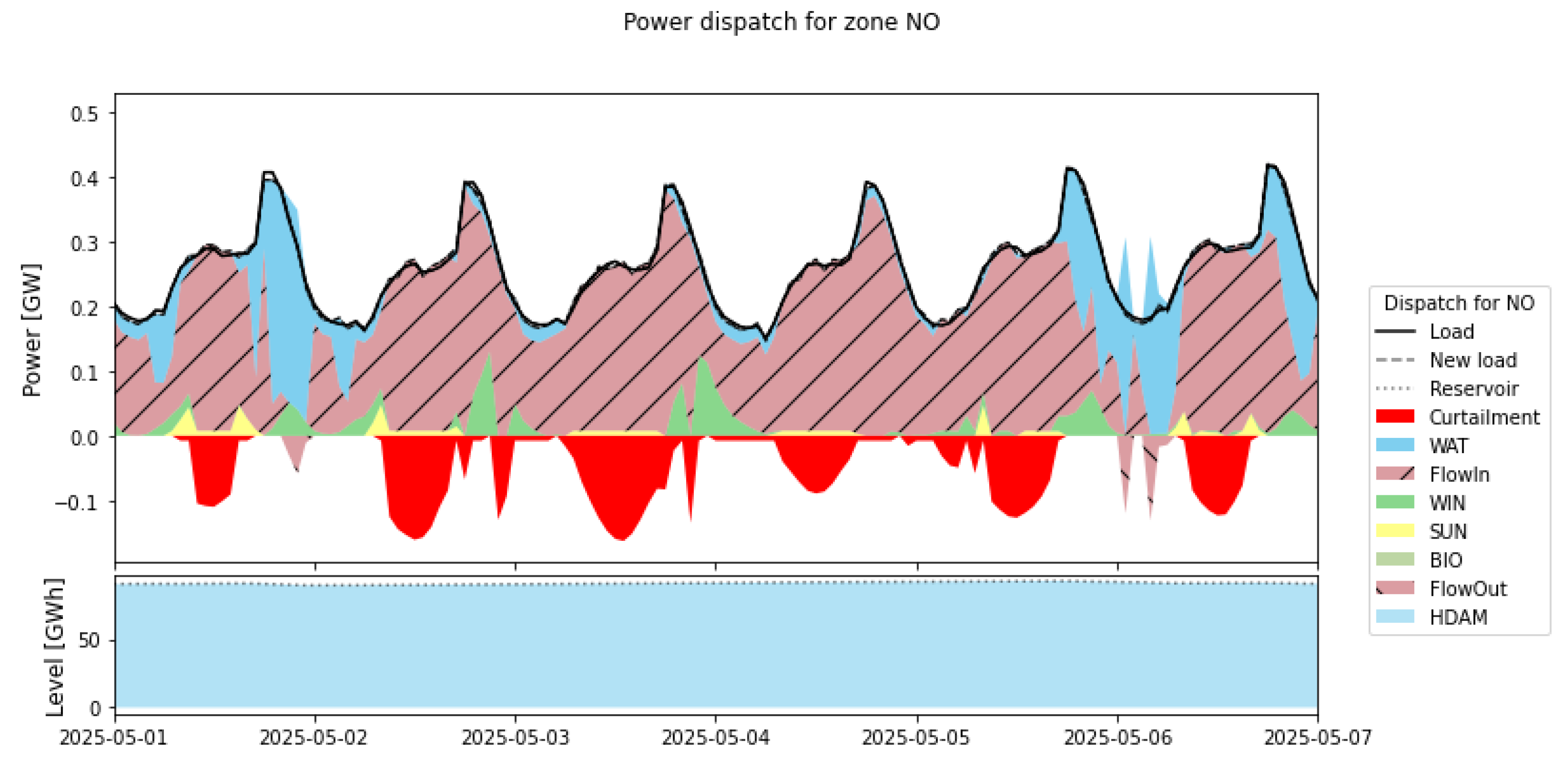
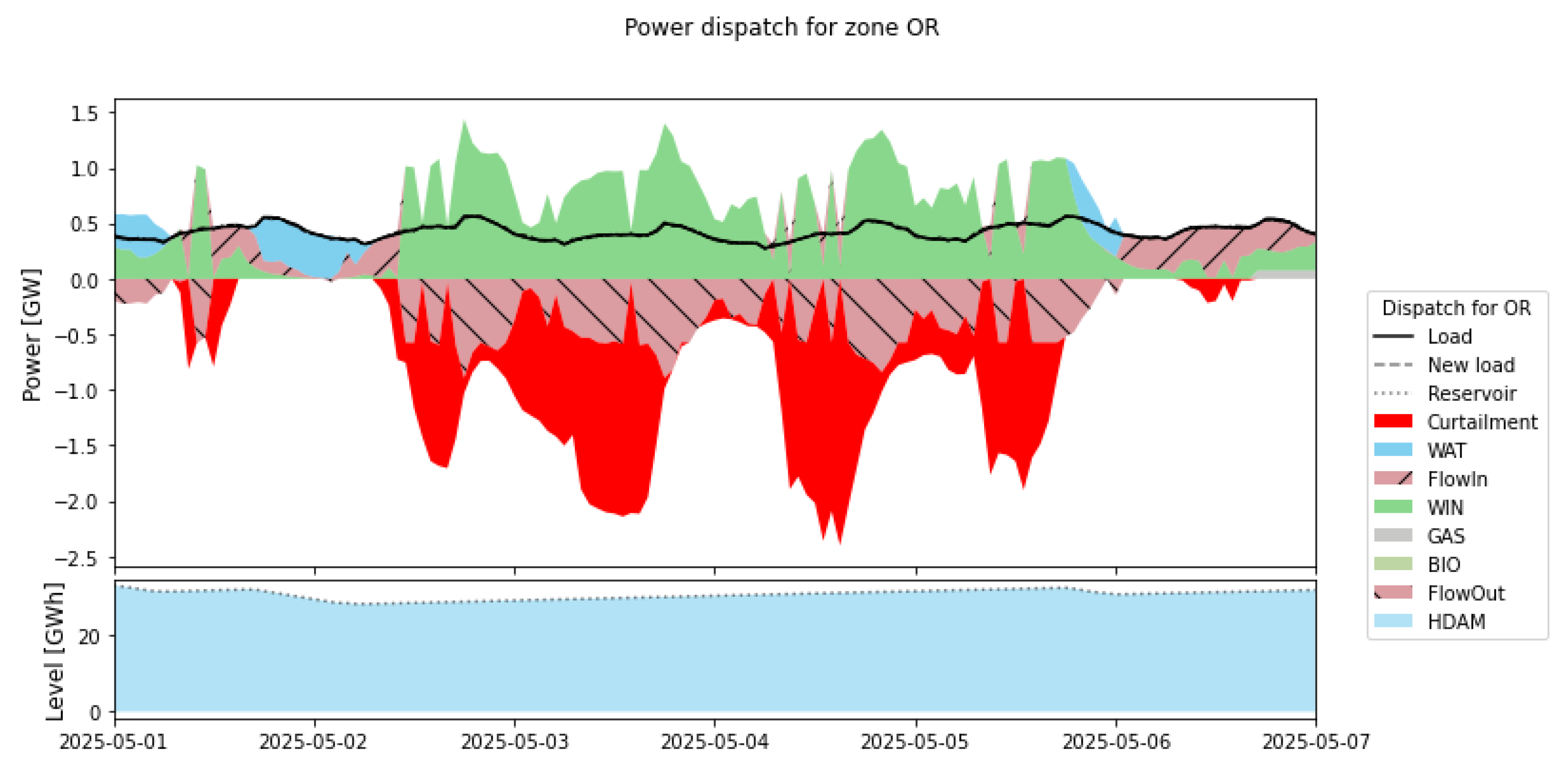
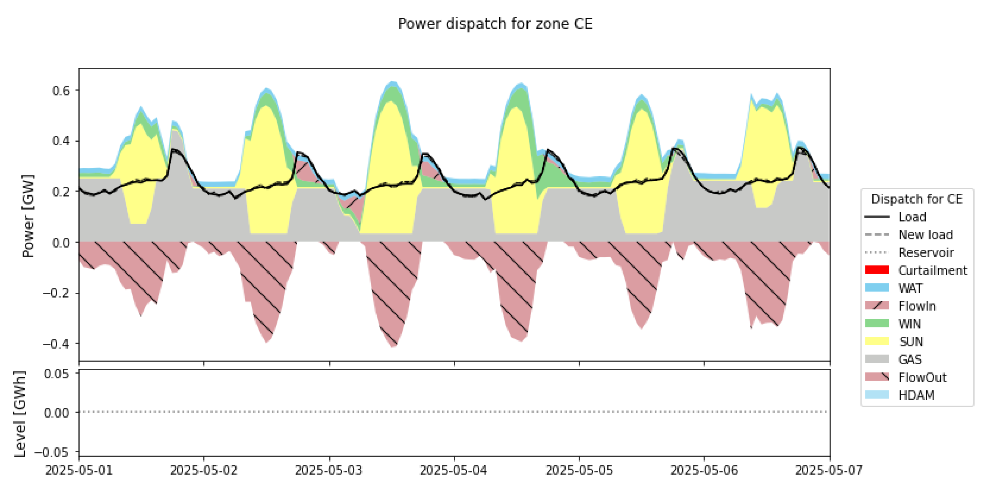
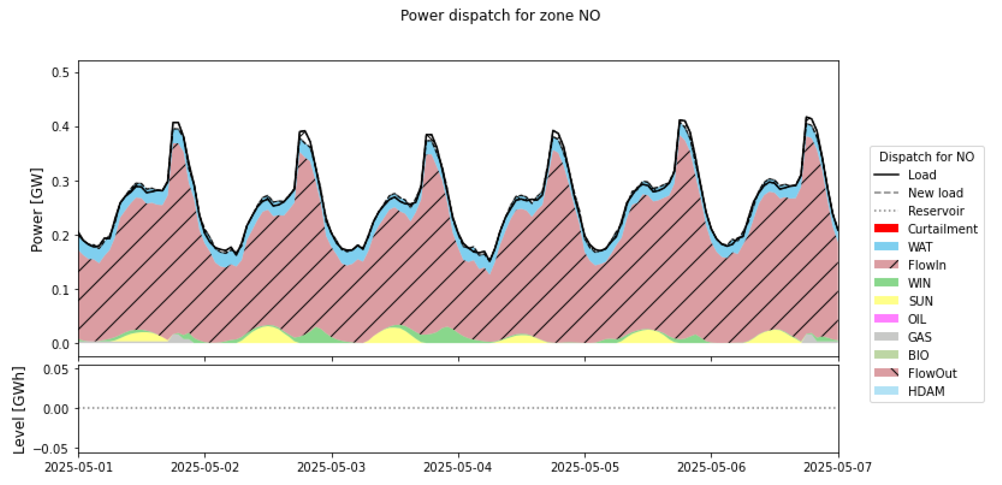
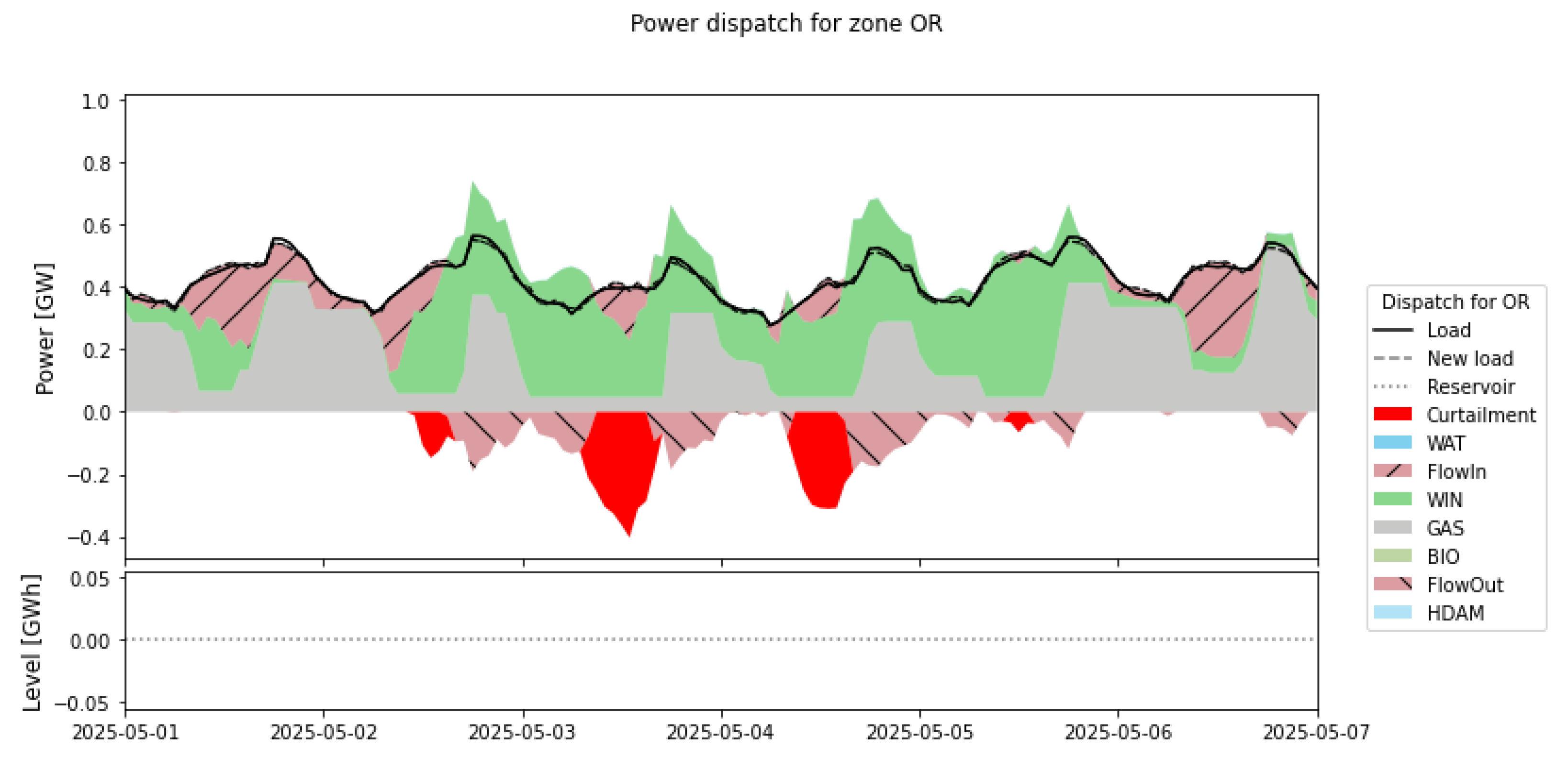
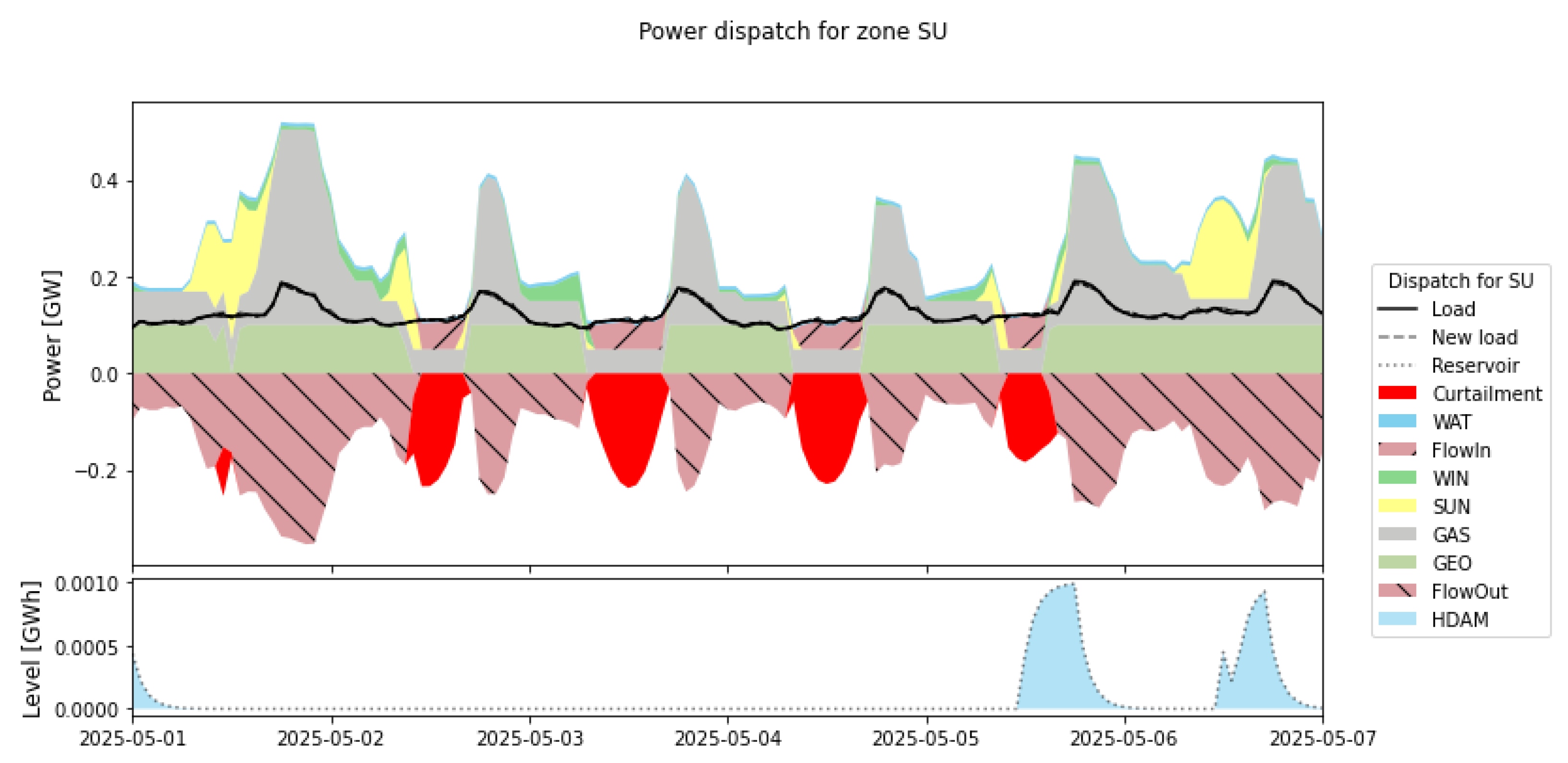
4.1. Accounting for the Flexibility of Hydro Reservoirs

The increment in VRES generation translates into a cascade of effects on the power system. They are described below.
Table 8 shows the assumed increments of VRES generation supply from 1.21 TWh in scenario 1(H) to 8.84 TWh in scenario 10(H). That represents an increase in the covered load by VRES from 10.31% to 75.29%.
High curtailment levels are obtained in the most ambitious scenarios, starting at 0.11 TWh for scenario 8(H) and reaching 10.08 TWh for scenario 10(H) (Table 7). The difference in the curtailment levels can be seen between the low-penetration Scenario and the Very-high-penetration scenario in the Figure 18, Figure 19, Figure 20, Figure 21, Figure 22, Figure 23, Figure 24 and Figure 25, where the red colored area is the curtailment of each zone.
Another important observation at the high-renewable-penetration level is the near disappearance of thermal generation, from 7.25 TWh for scenario 1(H) down to 0.18 TWh for scenario 10(H). This results in an important reduction in CO 2 emissions, from 2.11 Mt for scenario 1(H) to 0.09 Mt for scenario 10(H). This will accelerate the reduction of CO 2 emissions per capita, which in 2020 was 1.79 t [72]. Another substantial benefit is the reduction in the consumption of fuels (mostly natural gas), making it available for increased exportation.
Is important to notice in this dispatch strategy that the hydroelectric energy contribution remains almost constant, close to 3.2 TWh, which shows an important complementarity between VRES sources. This can be verified by the absence of Load Shedding as from scenario 4(H) in Table 7. We can also observe this in the Figure 18, Figure 19, Figure 20, Figure 21, Figure 22, Figure 23, Figure 24 and Figure 25, where the blue colored area is the HYDRO generation in each zone and appears normally before and after the solar energy (in yellow).
Table 9 shows that energy flows between zones mainly occur from Central to Oriental (CE –> OR), from North to Oriental (NO –> OR), from Oriental to North (OR –> NO), from Oriental to South (OR –> SU), and from South to Central (SU –> CE). The number of congestion hours is an important indicators of the need to increase its power capacity.
An additional observation from Table 9 is that the Oriental and South zones have a very low hydroelectric supply and storage capacity, which indicates less resilience and lower flexibility levels when incorporating VRES.
Finally, on the economic side, we can observe from Table 7 that the average power generation cost is reduced from 5.03 EUR/MWh in scenario 1(H) to 0.22 EUR/MWh in scenario 10(H), which is significant. However, the calculated cost does not consider the investment costs of new projects of the maintenance costs of power plants in operation.

4.2. Simulation Results without Hydro Reservoirs

Considering the same VRES installed power levels as in the previous dispatch strategy, the following is observed:
In Table 8, there could be even more increments of VRES generation supply than the strategy with hydro storage; from 1.21 TWh in scenario 1(NH) to 8.35 TWh in scenario 10(NH). This represents an increment in covered load by VRES from 10.35% to 71.18%.
This is observed in Figure 26, Figure 27, Figure 28, Figure 29, Figure 30, Figure 31, Figure 32 and Figure 33, where the peaks of the curves and areas colored in yellow (solar energy) and green (wind energy) are more pronounced and accentuated. However, this is explained by the fact that the hydro generation is almost zero, and there is no complementarity between hydro and VRES generation during periods with low availability of VRES. In Figure 26, Figure 27, Figure 28, Figure 29, Figure 30, Figure 31, Figure 32 and Figure 33, there are almost no areas colored with blue that mean that there is no supply of hydro generation.
Furthermore, because of the absence of hydro generation, the curtailment levels are greatly increased. It is null in scenario 1(NH) but reaches 9.63 TWh in scenario 10(NH). This is a similar value to the strategy with hydro storage (Table 6). Without hydro storage, the maximum levels of load shedding are 112.07 MWh. This is explained by the lack of hydro flexibility, which forces the start-up of thermal units to complement the variability of renewables.
Table 8 shows that the supply of thermal energy decreases from 9.97 TWh for scenario 1(NH) to 3.00 TWh for scenario 10(NH). Thermal generation is still significant, especially compared to the strategy with hydro storage. It results in relatively lower reduction of CO 2 emissions (from 3.21 Mt for scenario 1(NH) down to 0.59 Mt for scenario 10(NH)) and a lower reduction in the consumption of natural gas, which reduces the exportation potential for the country.
For this dispatch strategy, the hydroelectric supply and storage capacity is practically null, which clearly affects the robustness and flexibility by incorporating VRES, because the supply depends only on thermal and VRES generation.
Finally, on the economic side, we observe from Table 7 that the average operational costs are higher than in the strategy with hydro storage because of the large thermal generation used. Furthermore, they are less reduced than in the strategy with hydro storage (from 87.72 EUR/MWh in scenario 1(NH) down to 3.32 EUR/MWh in scenario 10(NH)).

5. Conclusions

This paper proposes the first open and comprehensive model of the Bolivian power system. The source code and input data are released under open licenses, thus ensuring a proper reproducibility and re-usability of this work.
In this work, a number of what-if scenarios with specific VRES expansion objectives are proposed. The goal is to assess the feasibility for the country to leapfrog towards a more renewable energy system instead of the current dependence on fossil fuels.
Simulation results show that high penetration of VRES can be obtained, reaching up to 75%. Furthermore, the installed thermal generation capacity could be displaced in 97%. This deployment of renewable energy, although technically feasible, is obtained at the expense of significant curtailment levels at VRES installed capacities higher than 2500 MW, corresponding to penetration levels higher than 180%.
The deployment of VRES presents important potential for operational costs reduction, with a decrease from 5.03 EUR/MWh down to 0.22 EUR/MWh. However, the importance of hydroelectric generation in economic terms is unquestionable, since the average cost of electricity without hydro storage reaches alarming values of 87.72 EUR/MWh in the worst-case scenario. It must, however, be noted that the investment costs for capacity expansion and the maintenance costs are not included in the simulations. The costs, although significant, remain acceptable when considering the very potential in renewable resources (mainly solar), thus resulting in leveled costs of electricity situated in the lower range of current estimates, which are already lower than traditional technologies in most regions of the world.
Load shedding could be significantly mitigated by the further deployment of VRES sources, thus contributing to the adequacy of the system. This is achieved through the contribution of hydro reservoirs to balance VRES variability. In contrast, in the strategy without hydro storage, the supply of energy is complemented by thermal generation, which results in higher CO 2 emissions.
For the strategy with hydro storage, the significant reservoir capacity present in the country allows a nearly complete displacement of thermal generation. On the other hand, for the strategy without hydro storage, the displacement of thermal generation is much lower, due to the fact that there is no hydro energy available to complement the supply during periods of low availability of VRES, and thermal generation is needed to cover the demand of energy.
The zone with maximum load-shedding levels is the oriental zone. This is the zone that has the largest demand and produces the least hydroelectric energy. Additionally, it has less storage capacity in hydro reservoirs. These features make the oriental zone less flexible in the face of abrupt changes in the supply of VRES due to its variability and therefore results in load shedding.
Results finally indicate the importance of increasing the power capacity of the transmission lines to/from the Oriental zone because they register the higher levels of hourly congestion. This is explained by the large thermal generation capacity and the lower importance of hydro units in that region: when VRESs are not sufficient to cover the demand, hydro generation is imported to the Iriental zone from other zones that have excess of hydro generation to supply their energy demands.

Author Contributions

Conceptualization, M.N. and S.Q.; methodology, M.N. and S.Z.; software, S.Q.; validation, R.O., M.V. and S.B.; formal analysis, M.N.; investigation, M.N. and S.Z.; resources, M.V.; data curation, M.N.; writing—original draft preparation, M.N.; writing—review and editing, S.B.; visualization, M.N. and S.B.; supervision, S.Q., R.O. and S.B. All authors have read and agreed to the published version of the manuscript. Please turn to the CRediT taxonomy https://www.mdpi.com/data/contributor-role-instruction.pdf, accessed on: 3 December 2021 for the term explanation.

Funding

This research was funded by the Flemish academic cooperation VLIR-UOS, South Initiative project BO2020SIN270A101. This financial support is gratefully acknowledged.

Institutional Review Board Statement

Not applicable.

Informed Consent Statement

Not applicable.

Data Availability Statement

All the source code, input data and results relative to this paper are available under open licences at https://github.com/CIE-UMSS/Dispa-SET_Bolivia, accessed on: 15 January 2022.

Conflicts of Interest

The authors declare no conflict of interest.

Abbreviations

The following abbreviations are used in this manuscript:
VRES  Variable Renewable Energy Sources
SIN  National Interconnected System
PEEBOL2025  Electrical Plan of the Plurinational State of Bolivia–2025
CNDC  National Energy Dispatch Committee
ENDE  Bolivian National Electricity Company
DSM  Demand side management
HDAM  Hydroelectric with dam reservoirs
HROR  Hydroelectric run of river
PHOT  Solar Photovoltaic
WTON  Onshore wind turbine
COMC  Combined cycle
GTUR  Gas turbine
STUR  Steam turbine
WAT  Hydro energy
SUN  Solar energy
WIN  Wind energy
BIO  Bagasse, Biodiesel, Biomass
GAS  Gas, as fuel
OIL  Oil, as fuel
CE  Central zone
NO  North zone
OR  Oriental zone
SU  South zone
UD  Unit Commitment
ED  Economic Dispatch
LP  Linear Programing
MILP  Mixed Interger Linear Programing
MINLP  Mixed Interger Non Linear Programming
UNEP  United Nations Environment Programme
COP  Climate Change Conference of the Parties
IRENA  International Renewable Energy Agency
NDC  Nationally Determined Contributions
HYTHCO  Hydro-Thermal Coordination
MO  Maintenance Optimization
GEP  Generation Expansion Planning
PCO  Production Cost Optimization
SIMSEE  Simulation of Electrical Power Systems Software
DEEM  Multinodal Stochastic Economic Dispatch Software
SDG  Sustainable Development Goals
MERRA-2  Modern-Era Retrospective analysis for Research and Applications, Version 2
PV  Photo-Voltaic

References

  1. United Nations. Paris Agreement; United Nations: Bonn, Germany, 2015. [Google Scholar]
  2. International Energy Agency. The Power of Transformation. Wind, Sun and the Economics of Flexible Power Systems; International Energy Agency (IEA): Paris, France, 2014. [Google Scholar]
  3. Bistline, J.; Blanford, G. The role of the power sector in net-zero energy systems. Energy Clim. Chang. 2021, 2, 100045. [Google Scholar] [CrossRef]
  4. United Nations. COP26 the Glasgow Climate Pact; United Nations: Bonn, Germany, 2021. [Google Scholar]
  5. International Renewable Energy Agency (IRENA). TIRENA Innovation and Technology Centre; A Roadmap to 2050; IRENA: Abu Dhabi, United Arab Emirates, 2019. [Google Scholar]
  6. United Nations. Nationally Determined Contributions under the Paris Agreement; United Nations: Bonn, Germany, 2021. [Google Scholar]
  7. International Renewable Energy Agency (IRENA). TIRENA Innovation and Technology Centre; REmap 2030 a Renewable Energy Roadmap; IRENA: Abu Dhabi, United Arab Emirates, 2014. [Google Scholar]
  8. International Energy Agency. IEA to Produce World’S First Comprehensive Roadmap to Net-Zero Emissions by 2050; International Energy Agency (IEA): Paris, France, 2021. [Google Scholar]
  9. Neetzow, P. The effects of power system flexibility on the efficient transition to renewable generation. Appl. Energy 2021, 283, 116278. [Google Scholar] [CrossRef]
  10. Denholm, P.; Arent, D.J.; Baldwin, S.F.; Bilello, D.E.; Brinkman, G.L.; Cochran, J.M.; Cole, W.J.; Frew, B.; Gevorgian, V.; Heeter, J.; et al. The challenges of achieving a 100% renewable electricity system in the United States. Joule 2021, 5, 1331–1352. [Google Scholar] [CrossRef]
  11. Makolo, P.; Zamora, R.; Lie, T.T. The role of inertia for grid flexibility under high penetration of variable renewables—A review of challenges and solutions. Renew. Sustain. Energy Rev. 2021, 147, 111223. [Google Scholar] [CrossRef]
  12. Koltsaklis, N.E.; Dagoumas, A.S. State-of-the-art generation expansion planning: A review. Appl. Energy 2018, 230, 563–589. [Google Scholar] [CrossRef]
  13. Poncelet, K.; Delarue, E.; Six, D.; Duerinck, J.; D’haeseleer, W. Impact of the level of temporal and operational detail in energy-system planning models. Appl. Energy 2016, 162, 631–643. [Google Scholar] [CrossRef] [Green Version]
  14. Klotz, E.; Newman, A.M. Practical guidelines for solving difficult mixed integer linear programs. Surv. Oper. Res. Manag. Sci. 2012, 18, 18–32. [Google Scholar] [CrossRef]
  15. Batlle, C. Análisis del Impacto del Incremento de la Generación de Energía Renovable no Convencional en los Sistemas Eléctricos Latinoamericanos Herramientas y Metodologías de Evaluación del Futuro de la Operación, Planificación y Expansión; Banco Interamericano de Desarrollo: Washington, DC, USA, 2014. [Google Scholar]
  16. Palacio, P.S.; Chaer, R. Plataforma de Simulacion de Sistemas de Energia Electrica; Instituto de Ingenieria Electrica (IIE): Montevideo, Uruguay, 2007. [Google Scholar]
  17. Pena, J. Exploring Low-Carbon Development Pathways for Bolivia; Energy Systems KTH-dES: Stockholm, Sweden, 2020. [Google Scholar]
  18. Nations, U. The Sustainable Development Goals Report. 2021. Available online: https://unstats.un.org/sdgs/report/2021/ (accessed on 15 January 2022).
  19. Toledo, Y. Inauguration of the First Phase of the Photovoltaic Solar Plant in Oruro; EnergyPress: Barrio Chacarilla Santa Cruz, Bolivia, 2019. [Google Scholar]
  20. Toledo, Y. The Third Wind Farm Is Inaugurated in Santa Cruz; EnergyPress: Chacarilla Santa Cruz, Bolivia, 2021. [Google Scholar]
  21. Estado Plurinacional de Bolivia, M.d.l.p. DECRETO SUPREMO N° 447, Procedimientos de RetribucióN, Registro, InscripcióN de Empresas Instaladoras y RecoleccióN de InformacióN de Generadores Distribuidos; Gaceta Oficial del Estado Plurinacional de Bolivia: La Paz, Bolivia, 2021. [Google Scholar]
  22. Mamani, R.; Hackenberg, N.; Hendrick, P. Efficiency of High Altitude On-shore Wind Turbines: Air Density and Turbulence Effects—Qollpana Wind Farm (Bolivia). Energy Clim. Chang. 2018, 2, 487. [Google Scholar] [CrossRef] [Green Version]
  23. Mamani, R.; Hendrick, P. Weather research & forecasting model and MERRA-2 data for wind energy evaluation at different altitudes in Bolivia. Wind Eng. 2021, 46, 177–188. [Google Scholar]
  24. Lopez, G.; Aghahosseini, A.; Bogdanov, D.; Mensah, T.N.; Ghorbani, N.; Caldera, U.; Rivero, A.P.; Kissel, J.; Breyer, C. Pathway to a fully sustainable energy system for Bolivia across power, heat, and transport sectors by 2050. J. Clean. Prod. 2021, 293, 126195. [Google Scholar] [CrossRef]
  25. Candia, R.A.; Subieta, S.L.; Ramos, J.A.; Miquélez, V.S.; Balderrama, J.G.; Florero, H.J.; Quoilin, S. Techno-economic assessment of high variable renewable energy penetration in the Bolivian interconnected electric system. In International Conference on Efficiency, Cost, Optimization, Simulation and Environmental Impact of Energy Systems, Ecos; Universidad Publica de Navarra: Pamplona, Spain, 2018. [Google Scholar]
  26. Han, X.; Chen, X.; McElroy, M.B.; Liao, S.; Nielsen, C.P.; Wen, J. Modeling formulation and validation for accelerated simulation and flexibility assessment on large scale power systems under higher renewable penetrations. Appl. Energy 2019, 237, 145–154. [Google Scholar] [CrossRef]
  27. Hua, B.; Baldick, R.; Wang, J. Representing operational flexibility in generation expansion planning through convex relaxation of unit commitment. IEEE Trans. Power Syst. 2017, 33, 2272–2281. [Google Scholar] [CrossRef]
  28. Lund, P.D.; Lindgren, J.; Mikkola, J.; Salpakari, J. Review of energy system flexibility measures to enable high levels of variable renewable electricity. Renew. Sustain. Energy Rev. 2015, 45, 785–807. [Google Scholar] [CrossRef] [Green Version]
  29. Quoilin, S.; Hidalgo Gonzalez, I.; Zucker, A. Modelling Future EU Power Systems under High Shares of Renewables. The Dispa-SET 2.1 Open-Source Model; Publications Office of the European Union: Luxembourg, 2017. [Google Scholar]
  30. Bussieck, M.R.; Meeraus, A. General Algebraic Modeling System, GAMS. In Modeling Languages in Mathematical Optimization; Springer: Boston, MA, USA, 2018; pp. 137–157. [Google Scholar]
  31. Pina, A.; Silva, C.; Ferrão, P. Modeling hourly electricity dynamics for policy making in long-term scenarios. Energy Policy 2011, 39, 4692–4702. [Google Scholar] [CrossRef]
  32. Mitchell, J.E. Branch-and-Cut Algorithms for Combinatorial Optimization Problems. Math. Sci. 1999, 1, 65–77. [Google Scholar]
  33. Wolsey, L. Integer Programming; John Wiley and Sons, Inc.: Hoboken, NJ, USA, 1998. [Google Scholar]
  34. Desrosiers, J.; Lübbecke, M.E. Branch-Price-and-Cut Algorithms. In Wiley Encyclopedia of Operations Research and Management Science (EORMS); John Wiley &Sons: Hoboken, NJ, USA, 2010. [Google Scholar]
  35. de Electricidad, V.; Alternativas, E. Plan Eléctrico del Estado Plurinacional de Bolivia–2025; Ministerio de Hidrocarburos y Energía: La Paz, Bolivia, 2014. [Google Scholar]
  36. Schröder, A.; Kunz, F.; Meiss, J.; Mendelevitch, R.; Von Hirschhausen, C. Current and Prospective Costs of Electricity Generation until 2050; Deutsches Institut für Wirtschaftsforschung (DIW): Berlin, Germany, 2013. [Google Scholar]
  37. Loisel, R.; Shropshire, D.; Thiel, C.; Mercier, A. Document the Travail Working Paper Flexibility assessment in nuclear energy dominated systems with increased wind energy shares. Hal Open Sci. 2014, DESNL14583, 1–71. [Google Scholar]
  38. Comité Nacional de Despacho de Carga (CNDC). Despacho de Carga Realizado. 2020. Available online: https://www.cndc.bo/media/archivos/boletindiario/dcdr_301220.htm (accessed on 9 October 2021).
  39. Energy Information Administration. Capital Cost Estimates for Utility Scale Electricity Generating Plants; U.S. Department of Energy: Washington, DC, USA, 2016. [Google Scholar]
  40. Van den Bergh, K.; Delarue, E. Cycling of conventional power plants: Technical limits and actual costs, TME Working Paper-Energy and Environment. Energy Convers. Manag. 2015, 97, 70–77. [Google Scholar] [CrossRef]
  41. Alberici, S.; Boeve, S.; van Breevoort, P.; Deng, Y.; Forster, S.; Gardiner, A.; Gastel, V.v.; Grave, K.; Groenenberg, H.; de Jager, D.; et al. Subsidies and Costs of EU Energy; Final Report; European Commission, Directorate-General for Energy: Brussel, Belgium, 2014. [Google Scholar]
  42. Comité Nacional de Despacho de Carga. Memoria Anual CNDC; Comité Nacional de Despacho de Carga (CNDC): Cochabamba, Bolivia, 2019. [Google Scholar]
  43. Agencia Nacional de Hidrocarburos. Información Actualizada Sobre Precios e Historiales de Tarifas de Hidrocarburos. 2020. Available online: https://www.anh.gob.bo/w2019/contenido.php?s=13 (accessed on 9 October 2021).
  44. Comité Nacional de Despacho de Carga (CNDC). Ley de Electricidad. 2020. Available online: https://www.cndc.bo/normativa/ley_electricidad.php (accessed on 17 October 2021).
  45. Comité Nacional de Despacho de Carga (CNDC). Demanda de Energía y Potencia. 2020. Available online: https://www.cndc.bo/media/archivos/boletindiario/bal_301220.htm (accessed on 6 October 2021).
  46. Comité Nacional de Despacho de Carga (CNDC). Datos Hidrológicos. 2020. Available online: https://www.cndc.bo/media/archivos/boletindiario/dathid_291220.htm (accessed on 30 October 2021).
  47. Comité Nacional de Despacho de Carga (CNDC). Evolución de los Embalses. 2020. Available online: https://www.cndc.bo/media/archivos/estadistica_anual/volumen_181220.htm (accessed on 16 October 2021).
  48. Empresa Nacional de Electricidad CORANI, ENDE CORANI. Memoria Anual ENDE CORANI; Empresa Nacional de Electricidad CORANI; ENDE CORANI: Cochabamba, Bolivia, 2019. [Google Scholar]
  49. Comité Nacional de Despacho de Carga (CNDC). Estadística Anual, Generación Bruta año 2014. 2014. Available online: https:www.cndc.bo/media/archivos/estadistica_anual/genbruta_2014.htm (accessed on 16 October 2021).
  50. Comité Nacional de Despacho de Carga (CNDC). Estadística Anual, Generación Bruta año 2020. 2020. Available online: https://www.cndc.bo/media/archivos/estadistica_anual/genbruta_2020.htm (accessed on 2 October 2021).
  51. Nacional de Electricidad VALLE HERMOSO, ENDE VALLE HERMOSO. Memoria Anual ENDE VALLE HERMOSO; Empresa Nacional de Electricidad VALLE HERMOSO; ENDE VALLE HERMOSO: Cochabamba, Bolivia, 2019. [Google Scholar]
  52. Empresa Nacional De Electricidad–Corporación, ENDE Proyectos en Estudio 2019. 2019. Available online: https://www.ende.bo/proyectos/estudio (accessed on 15 September 2021).
  53. Estado Plurinacional de Bolivia, Ministerio de Hidrocarburos y Energía, and Viceministerio de Electricidad y Energías Alternativas. Plan de Desarrollo de Energías Alternativas 2025. Viceministerio de Electricidad y Energías Alternativas, Bolivia; Estado Plurinacional de Bolivia, Ministerio de Hidrocarburos y Energias: La Paz, Bolivia, 2014. [Google Scholar]
  54. Fernandez, P. Turbinas Hidráulicas; Departamento de Ingeniería Eléctrica y Energética-Universidad de Cantabria: Cantabria, Spain, 2017. [Google Scholar]
  55. Lucano, M.; Fuentes, I. Evaluation of the Global Solar Radiation Potential in the Department of Cochabamba (Bolivia) Using Models of Geographic Information Systems and Satellite Images; Universidad Mayor de San Andres (UMSA): La Paz, Bolivia, 2010. [Google Scholar]
  56. Lucano, M.; Fuentes, I. Atlas de Radiación Solar Global de Bolivia; Universidad Mayor de San Andres (UMSA): La Paz, Bolivia, 2010. [Google Scholar]
  57. Manatechs. Hora de Salida y Puesta del Sol. 2018. Available online: https://salidaypuestadelsol.com/bolivia/cochabamba_1035.html (accessed on 9 September 2021).
  58. Miguel Fernández, G.; Rodriguez, R.O.; Terrazas, E. Cambio Climático, Agua y Energía en Bolivia; Departamento de Asuntos Económicos y Sociales de Naciones Unidas (DESA-United Nations)—ENERGÉTICA: Cochabamba, Bolivia, 2012. [Google Scholar]
  59. Fuentes, M.F. Estudio Sostiene que la Energía Solar es Factible en el 97% del Territorio Nacional; ENERGÉTICA: Cochabamba, Bolivia, 2012. [Google Scholar]
  60. Dateandtime.info. Coordenadas Goeográficas. 2017. Available online: http://dateandtime.info/es/citycoordinates.php?id=3901903 (accessed on 24 October 2021).
  61. Staffell, I.; Pfenninger, S. Renewables.ninja. 2018. Available online: www.renewables.ninja (accessed on 21 September 2021).
  62. Duffie, J.A.; Beckman, W.A. Solar Engineering of Thermal Processes; John Wiley and Sons, Inc.: Hoboken, NJ, USA, 2013. [Google Scholar]
  63. Climate data.org. Datos Climáticos Mundiales. 2017. Available online: https://es.climate-data.org/ (accessed on 6 September 2021).
  64. Asea Brown Boveri, S.A. Cuaderno de Aplicaciones Técnicas n° 10. Plantas Fotovoltaicas; Asea Brown Boveri, S.A.: Barcelona, Spain, 2011. [Google Scholar]
  65. Peña, D.A.; Segura, A.G. El Módulo Fotovoltaico; Universidad de Jaen: Jaen, Spain, 2017. [Google Scholar]
  66. Bergman, L.; Enocksson, A. Design of a PV System with Variations of Hybrid System at Addis Ababa Institute of Technology; KTH School of Industrial Engineering and Management: Stockholm, Sweden, 2015. [Google Scholar]
  67. 3TIER. Informe Final. Atlas Eólico de Bolivia. Un Proyecto para la Corporación Financiera Internacional; 3TIER: Seatle, WA, USA, 2009. [Google Scholar]
  68. Finance, D.B. Concept Note—Three Wind Farms in Bolivia; Ministry of Foreign Affairs of Denmark: Copenhagen, Denmark, 2016. [Google Scholar]
  69. windpower.org. El Efecto del Parque. 2018. Available online: http://drømstørre.dk/wp-content/wind/miller/windpowerweb/es/tour/wres/park.htm (accessed on 12 October 2021).
  70. TheWindPower.net. Manufacturers and Turbines. 2018. Available online: https://www.thewindpower.net/turbines_manufacturers_es.php (accessed on 19 October 2021).
  71. Empresa Nacional de Electricidad, S.A. Memoria Anual 2018; ENDE: Cochabamba, Bolivia, 2018. [Google Scholar]
  72. Datosmacro. Bolivia, Emisiones de CO2. 2021. Available online: https://datosmacro.expansion.com/energia-y-medio-ambiente/emisiones-co2/bolivia (accessed on 19 September 2021).
Figure 1. Time horizons of the optimization with the look-ahead period [29].
Energies 15 00968 g001
Figure 2. Flow chart of the implementation and processing steps [29].
Energies 15 00968 g002
Figure 3. The SIN layout implemented and planned in the period 2020–2025 [35].
Energies 15 00968 g003
Figure 4. Load curves for all four zones (1–7 May 2020).
Energies 15 00968 g004
Figure 5. Load curve for all four zones (1–7 November 2025).
Energies 15 00968 g005
Figure 6. Renewable energypotential [53].
Energies 15 00968 g006
Figure 7. Solar energy potential [53].
Energies 15 00968 g007
Figure 8. Average wind speeds [53].
Energies 15 00968 g008
Figure 9. Hydroelectric energy potential [53].
Energies 15 00968 g009
Figure 10. HYDRO ENERGY implemented and planned in the period 2020–2025 [35].
Energies 15 00968 g010
Figure 11. Hydro run-of-river Resources Availability Factor (year 2025) [35].
Energies 15 00968 g011
Figure 12. SOLAR ENERGY implemented and planned in the period 2020–2025 [35].
Energies 15 00968 g012
Figure 13. Solar Resource Availability Factor (year 2025).
Energies 15 00968 g013
Figure 14. Solar Resources Availability Factor (1 May 2025).
Energies 15 00968 g014
Figure 15. WIND ENERGY implemented and planned in the period 2020–2025 [35].
Energies 15 00968 g015
Figure 16. Wind Resource Availability Factor (year 2025).
Energies 15 00968 g016
Figure 17. Wind Resource Availability Factor (1 May 2025).
Energies 15 00968 g017
Figure 18. Low0Penetration Scenario 1(H)—Central zone (1–7 May 2025).
Energies 15 00968 g018
Figure 19. Low0Penetration Scenario 1(H)—North zone (1–7 May 2025).
Energies 15 00968 g019
Figure 20. Low-Penetration Scenario 1(H)—Oriental zone (1–7 May 2025).
Energies 15 00968 g020
Figure 21. Low-Penetration Scenario 1(H)—South zone (1–7 May 2025).
Energies 15 00968 g021
Figure 22. Very-High-Penetration Scenario 10(H)—Central zone (1–7 May 2025).
Energies 15 00968 g022
Figure 23. Very-High-Penetration Scenario 10(H)—North zone (1–7 May 2025).
Energies 15 00968 g023
Figure 24. Very-High-Penetration Scenario 10(H)—Oriental zone (1–7 May 2025).
Energies 15 00968 g024
Figure 25. Very-High-Penetration Scenario 10(H)—South zone (1–7 May 2025).
Energies 15 00968 g025
Figure 26. Moderate-Penetration Scenario 1(NH)—Central zone (1–7 May 2025).
Energies 15 00968 g026
Figure 27. Moderate-Penetration Scenario 1(NH)—North zone (1–7 May 2025).
Energies 15 00968 g027
Figure 28. Moderate-Penetration Scenario 1(NH)—Oriental zone (1–7 May 2025).
Energies 15 00968 g028
Figure 29. Moderate Penetration Scenario 1(NH)—zone south (1–7 May 2025).
Energies 15 00968 g029
Figure 30. Very-High-Penetration Scenario 10(NH)—Central zone (1–7 May 2025).
Energies 15 00968 g030
Figure 31. Very High Penetration Scenario 10(NH)—zone north (1–7 May 2025).
Energies 15 00968 g031
Figure 32. Very-High-Penetration Scenario 10(NH)—Oriental zone (1–7 May 2025).
Energies 15 00968 g032
Figure 33. Very-High-Penetration-Scenario 10(NH)—South zone (1–7 May 2025).
Energies 15 00968 g033
Table 1. Power units parameters [29].
DescriptionField NameUnitsValue
Power Capacity (for one unit)  PowerCapacityMWAccurate [35]
Unit nameUnit Accurate [35]
ZoneZone Accurate [35]
TechnologyTechnology Accurate [35]
Primary fuelFuel Accurate [35]
EfficiencyEfficiency%Reference [36]
Minimum up timeMinUpTimehReference [36]
Minimum down timeMinDownTimehReference [36]
Ramp-up rateRampUpRate%/minReferences [36,37,38]
Ramp-down rateRampDownRate%/min)References [36,37,38]
Start-up costStartUpCostEURReference [36]
No load costNoLoadCostEUR/hReferences [36,39]
Ramping costRampingCostEUR/MWReference [40]
Minimum loadPartLoadMin%References [2,36,41]
Efficiency at minimum loadMinEfficiency%Reference [35]
Start-up timeStartUPTimehReferences [2,36]
CO 2 intensityCO 2 IntensityTCO 2 /MWhReference [42]
Number of unitsNunits Accurate [35]
Table 2. Power generation units in 2020 [35].
Area Central NameTechnologyNumber of UnitsTotal Power (MW)
CentralMiguillas SystemHDAM WAT921.11
Corani System10280.35
Misicuni System3120
San Jose San Jose IIHROR WAT4124
Kanata17.54
Valle HermosoGTUR GAS8107.65
Carrasco3122.94
Bulo Bulo3135.41
Entre Rios4105.21
Entre RiosCOMC GAS3376.98
Oruro IPHOT SUN 50.01
Qollpana I & IIWTON WIN1027
NorthTaquesi SystemHDAM WAT289.19
Zongo System21188.04
QuehataHROR WAT21.97
KenkoGTUR GAS2-
El Alto246.19
TrinidadGTUR OIL1925.28
Rurrenabaque11.8
Yucumo10.35
San Borja21.8
Say21.62
San Ignacio de Moxos20.73
San BuenaventuraGTUR BIO15
OrientalGuaracachiCOMC GAS3192.92
Warnes2248.1
GuaracachiGTUR GAS5126.72
Santa Cruz238.07
Warnes5195.56
UnagroGTUR BIO114.22
Guabira121
IAG15
SouthYura SystemHROR WAT719.04
San JacintoHDAM WAT27.6
AranjuezGTUR GAS1033.76
Karachipampa1-
Del Sur4147.55
Del SurCOMC GAS2232.32
Uyuni ColchaKPHOT SUN2160.06
Yunchara25
SINAllAll Technologies1843187.09
Table 3. Conventional and renewable generation projects planned for the period 2020–2025 [35].
Area CentralTechnologySituationTotal
CentralOruro IIPHOT SUNProjected up to 202150.01
Qollpana IIIWTON WINProjected up to 202321
Sehuencas_juntasHDAM WATProjected up to 2025279.88
Banda AzulProjected up to 2025133.7
NorthGuayaramerinPHOT SUNProjected up to 20253
RiberaltaProjected up to 20255.8
Umapalca_PalilladaHDAM WATProjected up to 2025203
SanCristobal_
Anazani_SantaRosa
HROR WATProjected up to 202545
TiticacaWTON WINProjected up to 202521
OrientalSan JulianWTON WINProjected up to 202139.6
WARNES IProjected up to 202114.4
El DoradoProjected up to 202154
RositasHDAM WATProjected up to 2025400
Warnes IIWTON WINProjected up to 202521
SouthLa VentoleraWTON WINProjected up to 202524
Laguna ColoradaSTURProjected up to 2025100
CarrizalI_CarrizalII_CarrizalIIIHDAM WATProjected up to 2025346.5
Icla_MargaritaProjected up to 2025270
Table 4. Transmission Capacity between zones in 2020 [35].
Power Flow Direction From Central NameTo Central NameVoltage Level (kV)NTC (MW)
CE <—> NOSantivanezPalca I230430
SantivanezPalca II230
MazocruzVinto230
CE <—> ORCarrascoYapacani230500
CarrascoArboleda230
CE <—> SUCataviOcuri115207.5
SantivanezSucre230
SINAll CentralsAll Centrals230–1151137.5
Table 5. Transmission projects planned for the period 2020–2025 [35].
Power Flow Direction From Central NameTo Central NameVoltage Level (kV)NTC (MW)
OR <—> SUCamiriSucre I230300
CamiriSucre II230
NO <—> ORParaisoTroncos I230160
ParaisoTroncos II230
CE <—> SUSantivanezSucre I115300
SantivanezSucre II230
SINAll CentralsAll Centrals230–115760
Table 6. Scenarios.
Table 6. Scenarios.
TotalWith Hydro StorageWithout Hydro StorageProjected Installed Capacity
Installed Capacity
MW
Scenario Storage Capacity
MWh
Scenario Storage Capacity
MWh
Hydro
MW
Thermal
MW
VRES
MW
5225.11(H)1,239,1061(NH)02536.922286.18402
5493.12(H)1,239,1062(NH)02536.922286.18670
5761.13(H)1,239,1063(NH)02536.922286.18938
5895.14(H)1,239,1064(NH)02536.922286.181072
6029.15(H)1,239,1065(NH)02536.922286.181206
6163.16(H)1,239,1066(NH)02536.922286.181340
7165.17(H)1,239,1067(NH)02536.922286.182342
9965.18(H)1,239,1068(NH)02536.922286.185142
12,465.19(H)1,239,1069(NH)02536.922286.187642
12,465.110(H)1,239,10610(NH)02536.922286.187642
Table 7. Electricity Cost, Load Shedding, Curtailment.
Scenario Average
Electricity
Cost
EUR/MWh
Total Load
Shedding
TWh
Maximum
Load
Shedding
MWh
Total
Curtailed
RES
TWh
Maximum
Curtailed
RES
MW
VRES
Installed
Capacity
MW
1(H)5.030.000253.410.00017.65402
2(H)4.280.00000.000.00017.65670
3(H)3.580.000146.220.0033193.94938
4(H)3.250.000021.350.0139387.761072
5(H)2.950.000052.890.0424510.941206
6(H)2.660.00000.000.0992905.231340
7(H)2.630.000024.140.11001040.162342
8(H)1.010.00000.002.65003109.315142
9(H)0.500.00000.006.17005076.597642
10(H)0.220.00000.0010.08006310.4610,142
1(NH)87.720.0317112.070.00000.00402
2(NH)51.830.0227112.070.000011.53670
3(NH)34.170.0164112.070.0103268.24938
4(NH)28.290.0144112.070.0330429.761072
5(NH)23.040.0129112.070.0710538.311206
6(NH)18.710.0109112.070.1370665.731340
7(NH)18.120.0109112.070.1510705.552342
8(NH)6.700.0034112.072.68002561.695142
9(NH)4.870.0018112.075.97004419.697642
10(NH)3.320.0012112.079.63006308.8710,142
Table 8. Generation results for each technology.
ScenarioHYDROTHERMALVRESThermal GenerationCovered Load by
Gen
TWh
CO 2
Mt
Gen
TWh
CO 2
Mt
Gen
TWh
CO 2
Mt
Displaced
TWh
VRES
%
1(H)3.280.007.252.111.210.000.0010.31
2(H)3.270.006.441.812.020.000.8117.22
3(H)3.270.005.631.522.830.001.6224.13
4(H)3.270.005.241.393.220.002.0127.45
5(H)3.270.004.871.263.590.002.3830.61
6(H)3.270.004.511.143.950.002.7433.67
7(H)3.270.003.471.124.990.003.7842.54
8(H)3.210.001.350.437.170.005.9061.13
9(H)3.150.000.460.218.130.006.7969.25
10(H)2.720.000.180.098.840.007.0775.29
1(NH)0.510.009.973.211.210.000.0010.35
2(NH)0.510.009.172.892.020.000.8017.26
3(NH)0.510.008.382.612.820.001.5924.08
4(NH)0.510.008.002.473.200.001.9727.33
5(NH)0.510.007.642.353.570.002.3330.46
6(NH)0.510.007.302.243.910.002.6733.36
7(NH)0.510.006.322.224.890.003.6541.72
8(NH)0.480.004.181.467.070.005.7960.27
9(NH)0.410.003.381.107.940.006.5967.69
10(NH)0.380.003.000.598.350.006.9771.18
Table 9. Number of hours of congestion in each line.
ScenarioCE –> NOCE –> ORCE –> SUNO –> CENO –> OROR –> CEOR –> NOOR –> SUSU –> CESU –> OR
1(H)372606004735859235147531984928
2(H)233000004655369274551431799527
3(H)143322104594143285555561617229
4(H)14336000457437281857441651132
5(H)23345700456430275557981611120
6(H)2233830045085428275875163198
7(H)13341900455452283057401618147
8(H)9356770469348729065885153371
9(H)737357204665987298361451544103
10(H)8364985046331293311262061957169
1(NH)10236000459102353582826960
2(NH)15235900458302390609923830
3(NH)14239400461902235648320800
4(NH)16239400463602220652320060
5(NH)16243100472902194650119260
6(NH)16245400481702152652318570
7(NH)18247900480102128653418360
8(NH)152726005025217260163669250
9(NH)1328272049566892843639612803
10(NH)1528394048929683100646418537
Publisher’s Note: MDPI stays neutral with regard to jurisdictional claims in published maps and institutional affiliations.

