A Multiobjective Artificial-Hummingbird-Algorithm-Based Framework for Optimal Reactive Power Dispatch Considering Renewable Energy Sources

Abstract

This paper proposes a new artificial hummingbird algorithm (AHA)-based framework to investigate the optimal reactive power dispatch (ORPD) problem which is a critical problem in the capacity of power systems. This paper aims to improve the performance of power systems by minimizing two distinct objective functions namely active power loss in the transmission network and total voltage deviation at the load buses subjected to various constraints within multiobjective framework. The proposed AHA-based framework maps the inherent flight and foraging capabilities exhibited by hummingbirds in nature to determine the best settings for the control variables (i.e., voltages at generation buses, the tap positions of on-load tap-changing transformers (OLTCs) and the size of switchable shunt VAR compensators) to minimize the overall objective functions. A multiobjective optimal reactive power dispatch framework (MO-ORPD) considering renewable energy sources (RES) and load uncertainties is also proposed to minimize the individual objectives simultaneously. The competency and robustness of the proposed AHA-based framework is validated and tested on IEEE 14 bus and IEEE 39 bus test systems to solve the ORPD problem. Eventually, the results are compared with other well-known optimization techniques in the literature. Box plots and statistical tests using SPSS are performed and validated to justify the effectiveness of the proposed framework.

1. Introduction

With the rapid growth and development of power systems and the push to alleviate the load demand to a greater extent, there is a dire need of robust and optimal power system planning and operational studies. The stable and robust steady-state operation of a power system requires that its real and reactive power demands are met accordingly and that voltage profiles are kept within limits [1,2]. Power loss and voltage deviations must be kept to a minimum for a smooth operation and performance of the electric power system network (EPSN). For this, the main control variables that govern the voltage stability and power losses must be investigated and controlled in an optimal way to achieve minimum losses in the transmission network and voltage deviations at various load buses (PQ buses) in a system. Optimal placement and sizing of switchable shunt VAR compensators, as the key variables governing the voltage limits, should also be considered [3,4]. Moreover, generation bus (PV bus) voltages and inline on-load tap-changing transformers (OLTCs) are also the key variables when considering voltage stability and minimizing power losses in a network. In the context of a power system, this aspect is called reactive power management. From the past few years, the voltage performance of the system has drawn great attention. This index is normally termed as the voltage profile of the system. A normal range of 0.95 to 1.05 pu is considered to be within safe limits for PQ buses. Generation bus voltages are controlled by the system operator. The reactive power at the generating station is governed by an automatic generation control (AGC) loop by altering its reference set point. The voltage profile of a system bears a great dependency upon the tap settings of a tap-changing transformer, altering the voltage set points of PV buses and switching in or out the reactive power resources, i.e., the capacitors/reactors in the system. At the same time, system losses also depend on these control variables. These control variables are mainly considered to form an optimization problem. To properly allocate the taps of an OLTC, voltages of PV buses and sizes of static VAR compensators, a multiobjective optimization problem is considered to minimize the voltage deviations and system losses while considering various equality and inequality constraints. ORPD plays a decisive role in the economical and reliable operation of a power system.

ORPD is considered as a subproblem of optimal power flow (OPF), which accounts for the changes in reactive power flow in the system [5]. ORPD is characterized as a complex nonlinear, multimodal optimization problem of mixed-integer nonlinear programming (MINLP) involving both continuous (the voltages at PV buses and the size of switchable VAR compensators) and discrete (OLTC taps) variables. Most of the mathematical and statistical techniques fail to solve the complex nature of the ORPD problem, which is why most of the techniques used to solve the problem are metaheuristic. In the literature, several conventional methods, such as linear programming (LP), quadratic programming (QP), Newton–Raphson and dynamic programming (DP) methods, were used to solve the ORPD problem [6,7,8]. However, they took a relatively large number of iterations leading to long computational times. Moreover, these techniques do not guarantee a global optimal solution and often get stuck in local optima. Recent trends to solve power system network problems using metaheuristic have offered significant advantages over the conventional ones [9,10,11,12]. Different optimization techniques such as sine cosine [13], chaotic bat algorithm [14], teaching–learning-based algorithm (TLBO) [15], cuckoo search algorithm (CSA) [16], gravitational-based search algorithm (GSA) [17] and grey wolf optimizer (GWO) have been used to obtain the solution of the ORPD problem. These techniques have the advantages of not getting trapped in local optima and they can handle a greater number of variables and constraints with highly nonconvex, nonlinear objective functions with less execution time. Hybrid techniques including GWO-PSO [18], fractional PSO-GSA [19] and hybrid artificial physics-PSO [20] have also proven to be useful in finding optimal solution for ORPD with relatively less execution time and more optimized results. In a nutshell, a large number of metaheuristic optimization techniques have been implemented to address the ORPD problem and their superiority over deterministic and mathematical approaches is evident from the literature. However, there is still much room to investigate the ORPD problem to achieve better results with fast convergence towards optimal solutions.

Most of the studies have addressed only the active power loss as the main objective function [21], whilst some have also considered the total voltage deviation as an objective [22]. In this research work, two distinct objective functions, namely, the active power loss ($P_{\mathrm{loss}}$) and total voltage deviation ($V_{\mathrm{dev}}$), are considered independently and in multiobjective environment as well. The key contributions of the proposed work are stated below:

• The artificial hummingbird algorithm (AHA) is the latest, efficient and robust approach, and it has not been investigated for the optimization of the ORPD problem so far. A new ORPD optimization framework embedded with AHA is proposed for the minimization of $P_{\mathrm{loss}}$ and $V_{\mathrm{dev}}$.
• A multiobjective framework based on Pareto optimality, incorporating $P_{\mathrm{loss}}$ and $V_{\mathrm{dev}}$ together, is modeled and formulated to solve the MO-ORPD problem.
• The ORPD problem is investigated for a probabilistic modeling of load, solar PV and wind energy sources uncertainties.
• The statistical tests are performed using SPSS (Statistical Package for the Social Sciences) software to validate the effectiveness of the results obtained using the proposed framework.

To validate the performance of the algorithm, the ORPD problem is implemented on two standard IEEE test systems, namely, the IEEE 14 bus test system and the IEEE 39 bus test system. A comparative analysis in terms of best results and convergence rates is drawn with some of the famous optimization techniques reported in the literature to justify the robustness and efficacy of the proposed AHA-based framework considering single and multiobjective problems.

2. Problem Formulation

The main objectives involved in solving the ORPD problem is the active power loss minimization, namely, $P_{\mathrm{loss}}$ and the minimization of the total voltage deviation, namely, $V_{\mathrm{dev}}$ at all the PQ buses in the system. These two indices are governed by control parameters, which include the voltages at PV buses, the tap settings of an OLTC and the size of switchable shunt VAR compensators. The ORPD problem can be solved as a single objective function by considering $P_{\mathrm{loss}}$ or $V_{\mathrm{dev}}$ as the main objective. However, a multiobjective function can also be formulated by considering the active power losses and voltage profile improvement together as objectives. Based on this, a single objective function considering $P_{\mathrm{loss}}$ and $V_{\mathrm{dev}}$ independently and a multiobjective framework (MO-ORPD) considering Pareto optimality is formulated, subjected to the satisfaction of various equality and inequality constraints.

2.1. Minimization of $P_{\mathrm{loss}}$

One of the main objectives of the ORPD problem is to minimize active power loss in the power system network. The control variables that govern these losses are the voltages at PV buses, the tap setting of OLTCs in the transmission lines and VAR, provided by switchable shunt VAR compensators at PQ buses. These variables are taken as control variables and are stated below:

$$u=\left[V_{G1},\dots ,V_{N_G},T_1,\dots ,T_{N_T},Q_{C1},\dots ,Q_{N_C}\right],$$

(1)

where u is the independent variable vector, $V_G$ is the voltage at the PV bus, T is the tap settings of OLTCs, $Q_C$ is the reactive power provided by shunt VAR compensators, $N_G$ is the number of PV buses, $N_T$ represents the total number of taps of an OLTC and $N_C$ represents the total number of shunt VAR compensators. The dependent variables involve the real and reactive powers at PV buses and the voltages at all the PQ buses in the network given by

$$v=\left[P_{G1},Q_{G1},\dots ,Q_{N_G},V_{L1},\dots ,V_{N_L}\right],$$

(2)

where v is the dependent variable vector, $P_G$ is the real power at the PV bus, $Q_G$ is the reactive power at the PV bus, $V_L$ is the voltage at the PQ bus and $N_L$ is the number of PQ buses. The first objective function to be considered is the minimization of $P_{\mathrm{loss}}$ in the network. The optimal management of reactive power in the network creates more cushion for real power flows and decreases the real power losses in the network significantly. The objective function considering a $P_{\mathrm{loss}}$ minimization is stated in Ref. [23] as:

$$\begin{array}{cc}\hfill \mathrm{Minimize}{F}_1& =P_{\mathrm{loss}}(v,u),\hfill \\ & =\sum _{i=1}^{N_B}\sum _{j=1}^{N_B}{G}_{ij}\left[V_i^2+V_j^2-2V_i{V}_{j}cos{\delta }_{ij}\right],\hfill \end{array}$$

(3)

where $P_{\mathrm{loss}}$ is the total active power loss, $N_B$ is the total number of bus bars, $G_{ij}$ indicates the conductance between bus i and j, $V_i$ represents the voltage magnitude at bus i, $V_j$ represents the voltage magnitude at bus j and ${\delta }_{ij}$ is the angle between bus voltages i and j.

2.2. Minimization of $V_{\mathrm{dev}}$

The second objective to be considered in the ORPD problem is the minimization of the total voltage deviation at all the buses in the network. Voltages at all the PQ buses in the network must remain closer to 1.0 pu for the safe and reliable operation of the system and for ensuring enhanced service quality. The least voltage deviations at PQ buses correspond to an improved system voltage profile. The voltage profile is defined based on the index which is considered as the objective function in the minimization problem given as follows:

$$\begin{array}{cc}\hfill \mathrm{Minimize}{F}_2& =V_{\mathrm{dev}}(v,u),\hfill \\ \hfill & =\sum _{i=1}^{N_L}\left|V_i-V_i^{ref}\right|,\hfill \end{array}$$

(4)

where $V_{\mathrm{dev}}$ is the total voltage deviation at PQ buses and $V_i^{ref}$ is the reference voltage at PQ bus i, which is usually set at 1.0 pu.

2.3. Minimization of $P_{\mathrm{loss}}$ and $V_{\mathrm{dev}}$ a Considering Multiobjective Framework

The MO-ORPD problem is formulated to achieve the minimum active power losses in the network and minimum voltage deviations at the PQ buses in the network simultaneously as defined by

$$\begin{array}{cc}\hfill \mathrm{Minimize}{F}_3& =f(P_{\mathrm{loss}}(v,u),V_{\mathrm{dev}}(v,u)),\hfill \\ \hfill & =\left[F_1\left(P_{\mathrm{loss}}\right),F_2\left(V_{\mathrm{dev}}\right)\right].\hfill \end{array}$$

(5)

The MO-ORPD problem is solved using a multiobjective framework based on Pareto optimality, incorporating $P_{\mathrm{loss}}$ and $V_{\mathrm{dev}}$ together.

2.4. Constraints

The aforementioned objective functions defined as $F_1$, $F_2$ and $F_3$ are subjected to equality and inequality constraints. Equality and inequality constraints must be met for the reliable and secure operation of the power system. These constraints reflect the performance of the power system and restrain the voltages at all the buses in the network to remain within the defined limits.

2.4.1. Equality Constraints

Equality constraints are implemented through the power flow equations and are extensively deployed by power system planners [24,25].

$$P_i=V_i\sum _{k=1}^{N_B}{V}_j\left(G_{k}cos\left({\delta }_i-{\delta }_j\right)+B_{k}sin\left({\delta }_i-{\delta }_j\right)\right)=0,$$

(6)

$$P_i=P_{Gi}-P_{Di},$$

(7)

$$Q_i=V_i\sum _{k=1}^{N_B}{V}_j\left(G_{k}sin\left({\delta }_i-{\delta }_j\right)-B_{k}cos\left({\delta }_i-{\delta }_j\right)\right)=0,$$

(8)

$$Q_i=Q_{Gi}-Q_{Di},$$

(9)

where $B_k$ is the mutual susceptance of the kth branch (transmission line), $P_D$ is the active power demand at the PQ bus and $Q_D$ is the reactive power demand at the PQ bus.

2.4.2. Inequality Constraints

The inequality constraints must be restricted within their limits, which are defined in the following subsections.

Generator Constraints

The reactive power delivered by a generator and the voltage at the PV bus must be restricted within the limits given by

$$Q_{Gi}^{min}\le Q_{Gi}\le Q_{Gi}^{max},i\in N_G,$$

(10)

$$V_{Gi}^{min}\le V_{Gi}\le V_{Gi}^{max},i\in N_G,$$

(11)

where $Q_{Gi}^{min}$ and $Q_{Gi}^{max}$ are the minimum and maximum limits of the reactive power at PV buses and $V_{Gi}^{min}$ and $V_{Gi}^{max}$ are the minimum and maximum limits of the voltages at PV buses.

Load Angle Constraint

The load angle constraint is governed by the power transfer capability curve that indicates the maximum load angle to be equal to ${90}^{\circ }$ for maximum power transfer [26]. However, the stability of the system imposes a limit on this increase in angle, which, for practical purposes, is not considered above $45$–${60}^{\circ }$ . The load angle between two nodes i and j as defined by the following constraint is restricted to an angle of ${45}^{\circ }$.

$$-\frac{\pi }{4}\le {\delta }_i-{\delta }_j\le \frac{\pi }{4}.$$

(12)

Switchable Shunt VAR Compensator Constraint

The control variables defined for the reactive power injected by switchable shunt VAR compensators must be restricted within the limits given by

$$Q_{Ci}^{min}\le Q_{Ci}\le Q_{Ci}^{max},i\in N_C,$$

(13)

where $Q_{Ci}^{min}$ and $Q_{Ci}^{max}$ represent the minimum and maximum limits of the VAR injected by the shunt VAR compensator.

OLTC Constraint

The control variable defined for the tap setting of the on-load tap-changing transformer must be restricted within the limits given by

$$T_i^{min}\le T_i\le T_i^{max},i\in N_T,$$

(14)

where $T_i^{min}$ and $T_i^{max}$ are the minimum and maximum tap setting of ith OLTC.

System Constraints

The voltages at all the PQ buses in the network must be kept within the limits given by

$$V_i^{min}\le V_i\le V_i^{max},i\in N_B.$$

(15)

The real power at the slack bus must be kept within the limit defined by

$$P_s^{min}\le P_s\le P_s^{max},$$

(16)

where $P_s$ is the real power at the slack bus, $P_s^{min}$ is the minimum limit of the real power at the slack bus and $P_s^{max}$ is the maximum limit of the real power at the slack bus. The apparent power flow on the transmission line network must be restrained to a limit given by

$$S_k\le S_k^{max},k\in N_l,$$

(17)

where $S_k$ is the apparent power flow in kth branch, $S_k^{max}$ is the maximum permissible limit of the apparent power flow in kth branch and $N_l$ is the total number of branches (transmission lines).

2.5. Integration of Renewable Energy Sources in ORPD Problem

2.5.1. Scenario-Based Probabilistic Modeling

The integration of renewable energy sources (RES) into the power grid brings new challenges for power system planners [27,28,29]. The uncertainty and intermittency associated with the PV and wind plants make the ORPD problem more complex and stochastic in nature. Several probabilistic and analytical methods have been developed to evaluate the reliability and output power of the PV and wind generators. The output power from the PV and wind plants in this work were computed through a probabilistic modeling approach [30].

2.5.2. Solar PV Uncertainty Modeling

At a certain location and ambient temperature, the solar irradiance as well as the specifications of the PV module are important factors for determining the expected output power. The uncertainty in the irradiance patterns for solar PV is generated through a probability distribution function given by [31,32]

$$f_s\left(G_s\right)=\frac{1}{G_s{\sigma }_s\sqrt{2\pi }}exp\left[-\frac{{\left(ln{G}_s-{\mu }_s\right)}^2}{2{\sigma }_s^2}\right],G_s>0,$$

(18)

where $f_s$ is probability density function of solar irradiance, ${\mu }_s$ and ${\sigma }_s$ are the mean of the random variables and standard deviation and are considered to be equal to 5.5 and 0.5, respectively.

The power output of the solar PV as a function of irradiance can be computed using the following piecewise function

$$p_s\left(G_s\right)=\left\{\begin{array}{ccc}\hfill p_{sr}{G}_s^2/\left(G_{std}\times G_c\right)& \mathrm{for}& 0<G_s<G_c,\hfill \\ \hfill p_{sr}{G}_s/G_{std}& \mathrm{for}& G_s\ge G_c,\hfill \end{array}\right.$$

(19)

where $p_s,p_{sr}$ are the output and rated power of the solar plant (MW); $G_s,G_c$ and $G_{std}$ are the solar irradiance, specific irradiance point and standard solar irradiance of the environment ($\mathrm{W}/{\mathrm{m}}^2$). $G_{std}$ and $G_s$ are the standard solar irradiation at 1000 $\mathrm{W}/{\mathrm{m}}^2$ and the specific solar irradiance point set at 120 $\mathrm{W}/{\mathrm{m}}^2$, respectively. $p_{sr}$ is the PV array output power considered to be equal to 40 MW. The solar PV irradiance probability written as ${\tau }_{PV}$ is found using the irradiance uncertainty probability distribution function

$${\tau }_{\mathrm{PV},i}={\int }_{G_{s_{i,min}}}^{G_{s_{i,max}}}{f}_s\left(G_s\right)d{G}_s,$$

(20)

2.5.3. Wind Speed Uncertainty Modeling

The uncertainty in the wind speed is modeled using the Weibull distribution as given by [31,32]

$$f_w\left(v\right)=\left(\frac{\beta }{\alpha }\right){\left(\frac{v}{\alpha }\right)}^{\beta -1}exp\left[-{\left(\frac{v}{\alpha }\right)}^{\beta }\right],0<v<\infty ,$$

(21)

where $\alpha$ is the scale parameter, $f_w$ is the probability density function of the wind speed and $\beta$ is the shape parameter. $\alpha$ and $\beta$ are considered to be equal to 7.5 and 1.5, respectively, for the wind generator connected at bus 5.

The power output of the wind turbine as a function of wind speed (v) can be computed using the following piecewise function

$$p_w\left(v\right)=\left\{\begin{array}{ccc}\hfill 0& \mathrm{for}& 0\le v<v_i\hfill \\ \hfill p_{wr}\left(\frac{v-v_i}{v_r-v_i}\right)& \mathrm{for}& v_i\le v<v_r\hfill \\ \hfill p_{wr}& \mathrm{for}& v_r\le v<v_o\hfill \\ \hfill 0& \mathrm{for}& v\ge v_o\hfill \end{array}\right.,$$

(22)

where $p_w$ is the output power of the wind plant (MW), v is the wind speed (m/s), $p_{wr}$ is the rated power of the wind plant (MW) and $v_i,v_r$ and $v_o$ are the cut-in, measured and cut-out wind speeds (m/s), respectively. $p_w$ is the rated output power of the wind turbine considered to be equal to 4 MW for each of the 10 turbines, collectively making 40 MW for the wind generator. The wind speed probability for different wind scenarios is found using

$${\tau }_{\mathrm{wind},j}={\int }_{v_{j,min}}^{v_{j,max}}{f}_w\left(v\right)dv,$$

(23)

where $v_{j,min}$ and $v_{j,max}$ represent the start and end point of the wind speed’s interval at the jth scenario while ${\tau }_{\mathrm{wind},j}$ is the probability of the wind speed expected in the jth scenario.

2.5.4. Load Demand Uncertainty Modeling

The uncertainty in load demand is a challenging task in power systems and needs to be addressed and modeled using some probabilistic techniques. There are a number of techniques proposed in the literature to cater to a varying load demand. However, modeling the uncertainty in load using the normal distribution function is extensively used in research [33].

$$f_{\mathrm{load}}\left(P_d\right)=\frac{1}{{\sigma }_d\sqrt{2\pi }}exp{\left[-\frac{\left(P_d-{\mu }_d\right)}{{\sigma }_d\sqrt{2\pi }}\right]}^2,$$

(24)

where ${\sigma }_d$ and ${\mu }_d$ are the standard deviation and mean values considered to be equal to 75 and 12 for the simulations. $P_d$ represents the probability density of the load normal distribution. The probability of the load demand written as ${\tau }_{\mathrm{load}}$ with the expected load scenarios can be modeled as

$${\tau }_{\mathrm{load},k}={\int }_{P_{d_{k,min}}}^{P_{d_{k,max}}}{f}_{\mathrm{load}}\left(P_d\right)d{P}_d,$$

(25)

$$P_{d,k}={\int }_{P_{d_{k,min}}}^{P_{d_{k,max}}}\frac{P_d}{f_{\mathrm{load}}\left(P_d\right)}d{P}_d,$$

(26)

where $P_{d_{k,min}}$ and $P_{d_{k,max}}$ represent the minimum and maximum limits for the interval k.

2.5.5. Combined Load Generation Model

The combined irradiation, wind speed and load scenario probabilities can be written using (20), (23) and (25) as

$${\tau }_T={\tau }_{\mathrm{PV},i}\times {\tau }_{\mathrm{wind},j}\times {\tau }_{\mathrm{load},k},$$

(27)

In this paper, the three considered scenarios for solar irradiance, wind speed and load uncertainty generated with corresponding probabilities are given in

Table 1. Load, PV and wind scenarios and corresponding probabilities.

Load Scenario	Load (%)	${\mathit{\tau }}_{\mathbf{load},\mathit{k}}$
P1	20 (off-peak)	0.25
P2	40 (mid-peak)	0.7
P3	100 (on-peak)	0.05
PV Scenario	${\mathit{P}}_{\mathrm{PV}}$(MW)	${\mathit{\tau }}_{\mathrm{PV},\mathit{i}}$
S1	0	0.481
S2	0.485$p_{sr}$	0.374
S3	$p_{sr}$	0.145
Wind Scenario	${\mathit{P}}_{\mathrm{wind}}$(MW)	${\mathit{\tau }}_{\mathrm{wind},\mathit{j}}$
W1	0	0.073
W2	0.485$p_{wr}$	0.76
W3	$p_{sr}$	0.167

[33,34].

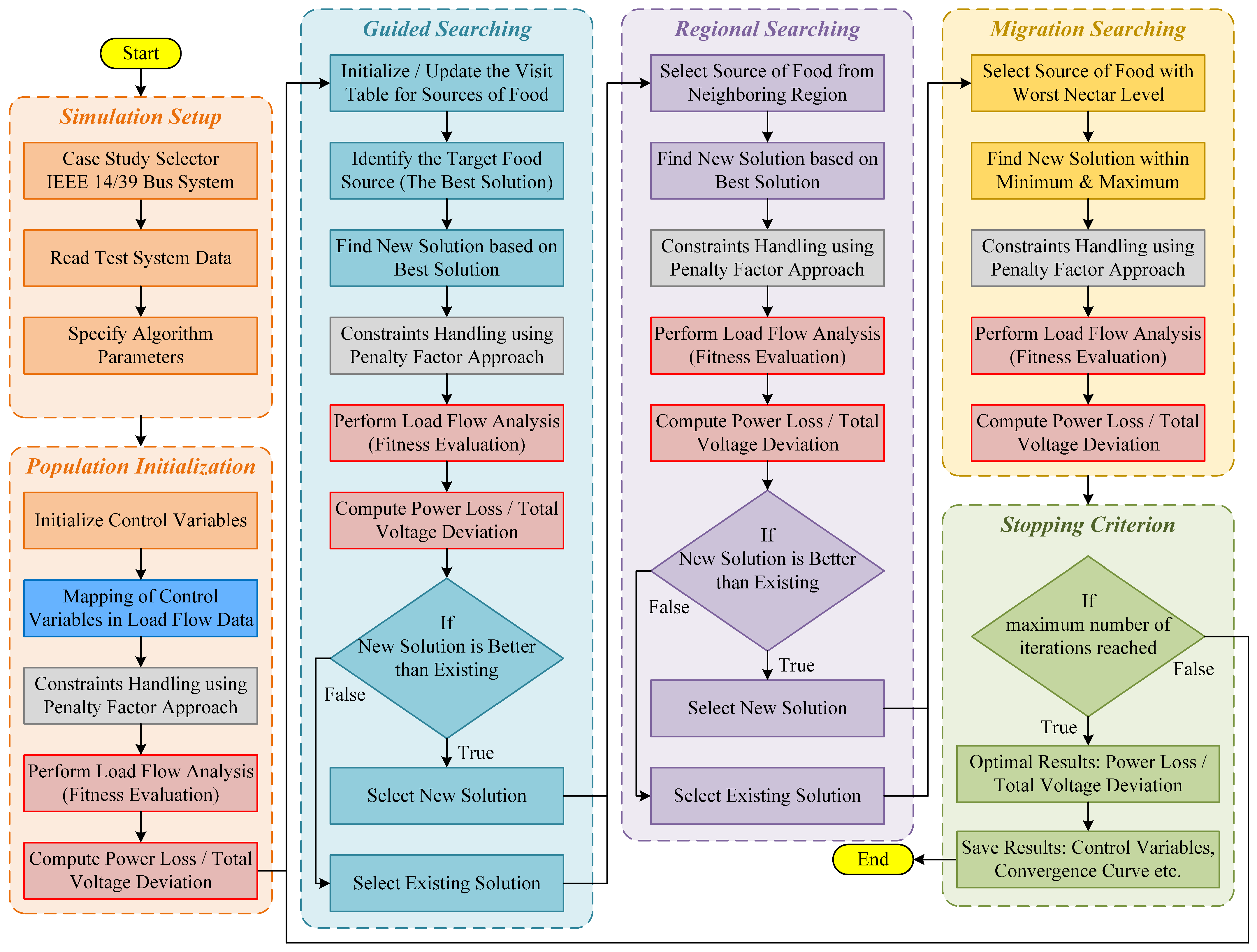
3. Artificial-Hummingbird-Algorithm-Based Framework for Optimal Reactive Power Dispatch Problem

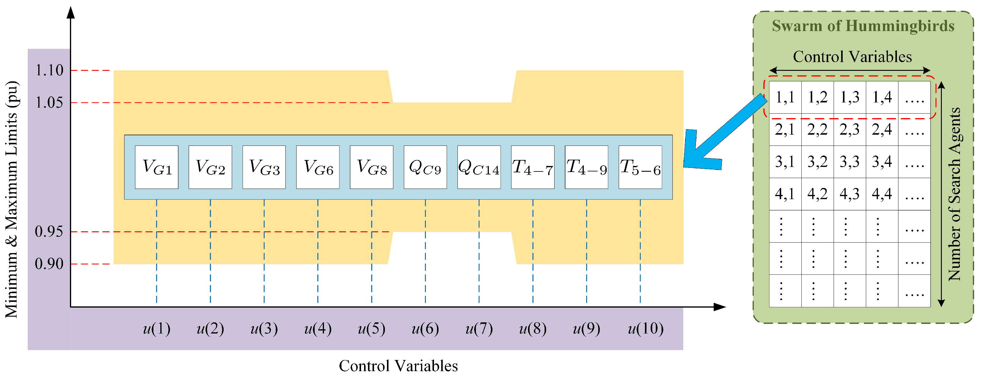
3.1. Mapping Procedure for Control Variables

The control variables that govern $P_{\mathrm{loss}}$ and $V_{\mathrm{dev}}$ are $V_G$, $Q_C$ and $T_T$. These control variables are mapped as a swarm of hummingbirds into the AHA framework to obtain the optimal control settings of the AGC, switchable VAR compensator and OLTC.

Figure 1 shows the control variables defined as $u\left(1\right)$, $u\left(2\right)$, …, $u\left(10\right)$ for the IEEE 14 bus test system, mapped into the columns of a population matrix of search agents wherein the rows indicate the population size. For instance, $u(3,4)$ in the population matrix indicates the value of $V_{G3}$ for the fourth search agent. The control variables are designated as floating-point values and integer values for continuous and discrete optimization problems, respectively. The minimum and maximum bounds for control variables are defined in terms of pu values. The mapping procedure for the IEEE 39 bus test system involves a similar approach for control variables spanning $u\left(1\right)$, $u\left(2\right)$, …, $u\left(21\right)$.

3.2. Artificial Hummingbird Algorithm

AHA is the newest bioinspired evolutionary optimization technique and algorithm which was recently developed by Weiguo Zhao in 2021 [35]. It illustrates the action of small hummingbirds to wisely search for food in their territory to gather the maximum amount of nectar. The food sources with enough amount of nectar become prominent among the swarm of hummingbirds. The hummingbirds fly to the sources, feed themselves on the flowers, pass to each other the information about the nectar level, keeping the information of the amount of nectar left in the mind, the number of rounds on the flowers, and the time since the most recent visit. The entire phenomenon has been exercised by hummingbirds for the foraging of food sources with the highest level of nectar, resulting in a close-optimal solution. Hummingbirds make moves in the search space with the help of three flight patterns: the axial movement of flight, diagonal movement flight, and omnidirectional movement of flight.

AHA is the population-based optimization algorithm in which the food sources for hummingbirds illustrate the key population for optimizing the problem. The food sources are represented as the solution to the ORPD problem given by

$$\begin{array}{c}P=\left[\begin{array}{cccccc}{H}_1^K& H_2^K& \cdots & H_m^k& \cdots & H_M^K\end{array}\right],\\ k=\left\{1,2,3,\cdots K\right\},\end{array}$$

(28)

where $H_m^k$ is mth variable of the kth search agent, P is the matrix of the population, K is the maximum number of variables and M is the vector-width of variables. The fitness value is calculated using the nectar availability index for the flowers (food sources). The best nectar availability index (NAI) is represented by the best fitness evaluation of the objective function regarding the evaluation of $P_{\mathrm{loss}}$ and $V_{\mathrm{dev}}$. The fitness in terms of NAI is given by

$$\begin{array}{c}{C}_k=f\left(H_1^k,H_2^k,H_3^k,\cdots H_M^k\right),\\ k=\left\{1,2,3,\cdots K\right\},\end{array}$$

(29)

where $C_k$ is the cost of the kth search agent. The entire process of searching for food is classified into three phases: guided searching, regional searching and migration searching. In guided searching, hummingbirds try to fly to the food sources with a higher value of NAI. Within the population of food sources, the sources with the best NAI value are nominated as the targeted food source. Analyzing the targeted source, the sources under consideration by a hummingbird is upgraded depending on the value of NAI and the unvisited time span. The guided searching can be characterized by

$${H_{new}}_m^k=H_m^{k,tar}+\alpha \times D\times \left(H_m^k-H_m^{k,tar}\right),\forall k,\forall m,$$

(30)

$${H_{new}}_m^k=\left\{\begin{array}{ccc}{H}_m^k& \mathrm{if}& f\left(H_m^k\right)\le f\left({H_{new}}_m^k\right),\\ {H_{new}}_m^k& \mathrm{if}& f\left(H_m^k\right)>f\left({H_{new}}_m^k\right),\end{array}\right.$$

(31)

where $\alpha$ is the guidance factor, $H_{new}$ is a freshly generated search agent, $H_m^{k,tar}$ is the target search agent and D is the flight style. In regional searching, hummingbirds travel to another zone of the region for targeting the next food sources with a better NAI compared to the last ones. This behavior is clearly illustrated in the local search of the algorithm and is given by the following equation

$${H_{new}}_m^k=H_m^k+\beta \times D\times H_m^k,\forall k,\forall m,$$

(32)

where $\beta$ is the regional factor. The exercise of migration searching results from a lack of food sources in a region and hummingbirds travel to another distinct region. The exploration feature for the search for further sources is a random generation within specified limits. The flowchart of the AHA is exhibited in Figure 2.

3.3. Multiobjective Artificial Hummingbird Algorithm (MO-AHA)

In the conventional AHA algorithm, the fitness value of a solution is evaluated by performing the guided foraging and territorial foraging, the current solution is iteratively replaced by better candidate solutions to achieve a global optimum solution. On the other hand, the MO-AHA [36] optimizes the multiple objective functions simultaneously using a dominance relation subject to some constraints, towards an optimized Pareto front solution. In the MO-AHA, a solution update strategy based on the NDS (nondominated solution) is utilized to achieve the true Pareto Front. The solution update strategy can be defined in the form of the equation given by

$${H_{new}}_m^k=\left\{\begin{array}{cc}{v}_{new}^k\hfill & p<q\hfill \\ H_m^k\hfill & p>q\hfill \\ v_{new}^k\hfill & p=q\mathrm{and}\mathrm{rand}<0.5\hfill \\ H_m^k\hfill & p=q\mathrm{and}\mathrm{rand}\ge 0.5\hfill \end{array}\right.$$

(33)

where $v_i\in F_p$, $x_i\in F_q$ and $F_p$ is the pth front, $F_q$ is the qth front in the NDS and $v_{new}^k$ is the updated velocity of the ${H_{new}}_m^k$ search agent.

3.4. Constraints Handling Using Penalty Factor Approach

The resulting optimization problem defined by $F_1$, $F_2$ and $F_3$ subjected to equality constraints (load flow equations) and inequality constraints (PV bus voltage control, OLTC tap setting, switchable shunt VAR compensator and other system constraints) were solved using the proposed optimization technique. A penalty factor approach was used for evaluating the objective function. Penalty factors for various constraints handling with penalized fitness function could be written as defined by

$$F\left(x\right)=F_1\left(x\right)+F_2\left(x\right)+{\beta }_P+{\beta }_Q+{\beta }_{\mathrm{C}}+{\beta }_T,$$

(34)

where

$${\beta }_P={\alpha }_1\sum _{i=1}^{N_B}\left\{P_{Gi}-P_{Di}-\left(\sum _{j=1}^{N_B}{V}_i{V}_j{Y}_{ij}\times cos\left({\theta }_{ij}-{\delta }_i+{\delta }_j\right)\right)\right\},$$

(35)

$${\beta }_Q={\alpha }_2\sum _{i=1}^{N_B}\left\{Q_{Gi}-Q_{Di}-\left(\sum _{j=1}^{N_B}{V}_i{V}_j{Y}_{ij}\times sin\left({\theta }_{ij}-{\delta }_i+{\delta }_j\right)\right)\right\},$$

(36)

$${\beta }_C={\alpha }_3\sum _{i=1}^{N_G}max\left\{0,Q_C-Q_C^{max}\right\}+{\alpha }_3\sum _{i=1}^{N_G}max\left\{0,Q_C^{min}-Q_C\right\},$$

(37)

$${\beta }_T={\alpha }_4\sum _{i=1}^{N_T}max\left\{0,T_i-T_i^{max}\right\}+{\alpha }_4\sum _{i=1}^{N_T}max\left\{0,N_T^{min}-N_i\right\},$$

(38)

$${\beta }_V={\alpha }_5\sum _{i=1}^{N_G}max\left\{0,V_i-V_i^{max}\right\}+{\alpha }_5\sum _{i=1}^{N_G}max\left\{0,V_i^{min}-V_i\right\},$$

(39)

where ${\alpha }_1$, ${\alpha }_2$, ${\alpha }_3$, ${\alpha }_4$ and ${\alpha }_5$ are the penalty factors, $Y_{ij}$ indicates the admittance between bus i and j and $F\left(x\right)$ is the penalized fitness function. A flow chart illustrating the steps to solve the ORPD problem is shown in Figure 3.

4. Simulation Results and Discussion

The efficacy and capability of the proposed AHA based framework were validated through various numerical and statistical studies. In this paper, the ORPD problem was implemented on two standard IEEE test systems namely the 14 bus test system and 39 bus test system, and the results were then compared with various other studies. The results obtained in this paper confirmed the efficacy of the proposed framework over other studies. Two objective functions were considered in this study: $P_{\mathrm{loss}}$ and $V_{\mathrm{dev}}$.

The maximum number of iterations for both test systems was set to 500 and the population size of hummingbirds was set to 100. The parameters were tuned to optimize the results and ensure that convergence was achieved. It is to be noted that all the tests were performed in MATLAB 2020b on an Intel(R) Core (TM) i7-5600U CPU with 8 Gb RAM and a 2.60 GHz processor.

4.1. IEEE 14 Bus Test System Considering Minimization of $P_{\mathrm{loss}}$

The efficacy of the proposed AHA-based framework was tested and validated using the IEEE 14 bus test system [37]. The test system contained 10 control variables, i.e., the decision variables including five PV buses, three OLTCs and two switchable shunt VAR compensators, which were to be optimized in a way to achieve a minimum $P_{\mathrm{loss}}$ in the network and a minimum $V_{\mathrm{dev}}$ at all the PQ buses in the network. The system contained five PV buses, three OLTCs and two switchable shunt VAR compensators, which were to be optimized as given in

Table 2. Technical parameters of IEEE 14 bus test system.

Sr. No.	Parameter	Value
1	Generators	5
2	Branches	20
3	OLTC	3
4	Shunt VAR compensators	2
5	Control variables	10

. The six PV buses were located at buses 1, 2, 3, 6 and 8, three inline OLTCs at branches 4–7, 4–9 and 5–6 and two switchable shunt VAR compensators at buses 9 and 14 in the network. Buses 4, 5, 7, 9, 10, 11, 12, 13 and 14 were PQ buses and were considered to be the candidate buses for the reactive power compensation. The voltages at all the PQ buses were constrained to remain within the limits of 0.9–1.1 pu at a 100 MVA base. Moreover, the transformer tap positions were restricted between 0.95 and 1.05 pu, and the permissible values for the shunt VAR compensators were constrained in the range of 0.9–1.1 pu.

In the first case, the proposed framework was implemented on IEEE 14 bus test system with the objective to achieve minimum active power losses as defined by (3). The results for the control variables and $P_{\mathrm{loss}}$ with reference to the base case, AHA and several other well-known optimization techniques implemented in other research studies are listed and compared in

Table 3. Optimal values of control variables with $P_{\mathrm{loss}}$ as an objective function for the IEEE 14 bus test system.

Control Variable	Base Case	SFO [18]	GWO-PSO [18]	CBA-4 [14]	SCA [10]	AHA
$V_{G1}$	1.0600	1.0171	1.0534	1.0921	1.09	1.0999
$V_{G2}$	1.0450	0.9909	1.0600	1.0884	1.08	1.0863
$V_{G3}$	1.0100	0.9520	0.9400	1.0588	1.05	1.0899
$V_{G6}$	1.0700	1.0099	0.9525	1.0325	1.09	1.0999
$V_{G8}$	1.0900	1.0279	0.9561	1.0951	1.09	1.0872
$Q_{C9}$	0.1800	-	-	0.2208	0.15	0.2917
$Q_{C14}$	0.1800	-	-	0.0786	0.06	0.0712
$T_{4-7}$	0.9780	0.9980	0.9972	0.9746	0.95	1.0034
$T_{4-9}$	0.9690	0.9867	0.9623	1.0676	0.94	0.9498
$T_{5-6}$	0.9320	0.9788	0.9882	1.0599	1.03	0.9874
$P_{\mathrm{loss}}$ (MW)	13.43	13.2786	13.2716	12.2923	12.27	12.2349
$V_{\mathrm{dev}}$ (pu)	0.0278	-	-	0.05308	-	0.0821

along with the corresponding values of $V_{\mathrm{dev}}$ when $P_{\mathrm{loss}}$ was considered as an objective function.

The proposed AHA-based framework showed a significant reduction in $P_{\mathrm{loss}}$ compared to the base case and other optimization techniques including SFO, GW-PSO and hybrid CBA-4. The efficacy and superiority of the AHA is evident from Figure 4, where a visual representation of $P_{\mathrm{loss}}$ is provided and compared with other optimization techniques. With $P_{\mathrm{loss}}$ as an objective function, the voltages at all the generation buses and load buses remained well within their limits where $V_{\mathrm{dev}}$ was found to be equal to 0.0821 pu.

4.2. IEEE 14 Bus Test System Considering Minimization of $V_{\mathrm{dev}}$

The proposed framework was implemented to achieve the minimum $V_{\mathrm{dev}}$ at all the PQ buses in the network as defined by (4). The results for the control variables, $V_{\mathrm{dev}}$ and the corresponding $P_{\mathrm{loss}}$ were compared with other optimization techniques as presented in

Table 4. Optimal values of control variables with $V_{\mathrm{dev}}$ as an objective function for the IEEE 14 bus test system.

Control Variable	Base Case	SFO	GWO-PSO	CBA-4	AHA
$V_{G1}$	1.06	0.94	1.06	0.9958	1.0776
$V_{G2}$	1.045	0.94	0.982	1.0189	1.0396
$V_{G3}$	1.01	1.06	1.0331	1.0008	0.9982
$V_{G6}$	1.07	0.94	1.06167	1.0102	1.0161
$V_{G8}$	1.09	1.06	1.0225	1.0501	0.9533
$Q_{C9}$	0.18	0.2	0.2	0.0903	0.2485
$Q_{C14}$	0.18	0.05	0.005	0.0637	0.1604
$T_{4-7}$	0.978	1.1	1.1	1.0121	1.0973
$T_{4-9}$	0.969	1.1	1.1	1.0975	0.9
$T_{5-6}$	0.932	0.9	0.9	1.037	0.9366
$P_{\mathrm{loss}}$ (MW)	13.43	-	-	15.9506	14.934
$V_{\mathrm{dev}}$ (pu)	0.0278	0.2133	0.2133	0.033	0.00152

. As in the first case, 25 simulation tests were performed, and the best results were tabulated.

The proposed AHA-based framework showed a significant reduction in voltage deviations compared to the base case and other optimization approaches including SFO, GW-PSO and hybrid CBA-4. The proposed AHA-based framework reflected the superiority and effectiveness of the algorithm compared to other approaches as shown in Figure 4. The voltage profile improvement is evident from the Figure 5, where the voltages at the PV buses and all the PQ buses in the network were found to be closer to unity represented by the dotted line.

The convergence curves for the IEEE 14 bus test system considering $P_{\mathrm{loss}}$ and $V_{\mathrm{dev}}$ as an objective function is shown in Figure 6, where the algorithm reached the optimal solution in 130 iterations and 180 iterations, respectively. The maximum number of iterations for the algorithm was set to 250. The fast convergence rate of the AHA compared to other optimization algorithms showed its better performance and effectiveness.

The complexity of the algorithm depended on the number of functional evaluations that directly affected the execution time. The execution time of the AHA for the IEEE 14 bus test system was 71 s, which was far better than some other techniques proposed in the literature [5]: differential evolution (145 s), whale optimization algorithm (140 s), PSO (103 s) and sine cosine algorithm (90 s). The minimum execution time of the AHA revealed that the said algorithm was effective at solving the optimization problems with less computational burden to reach optimal results.

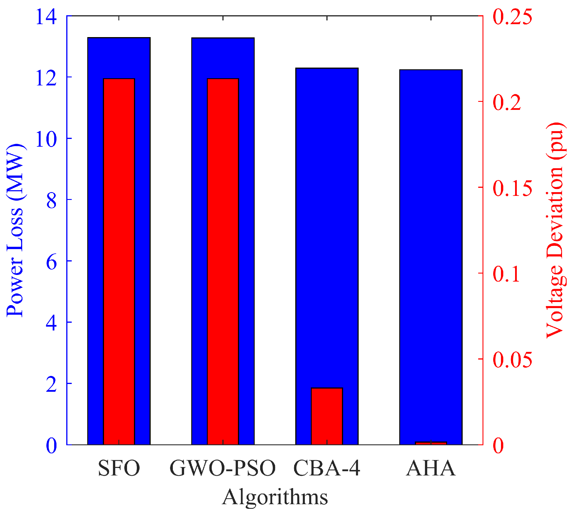
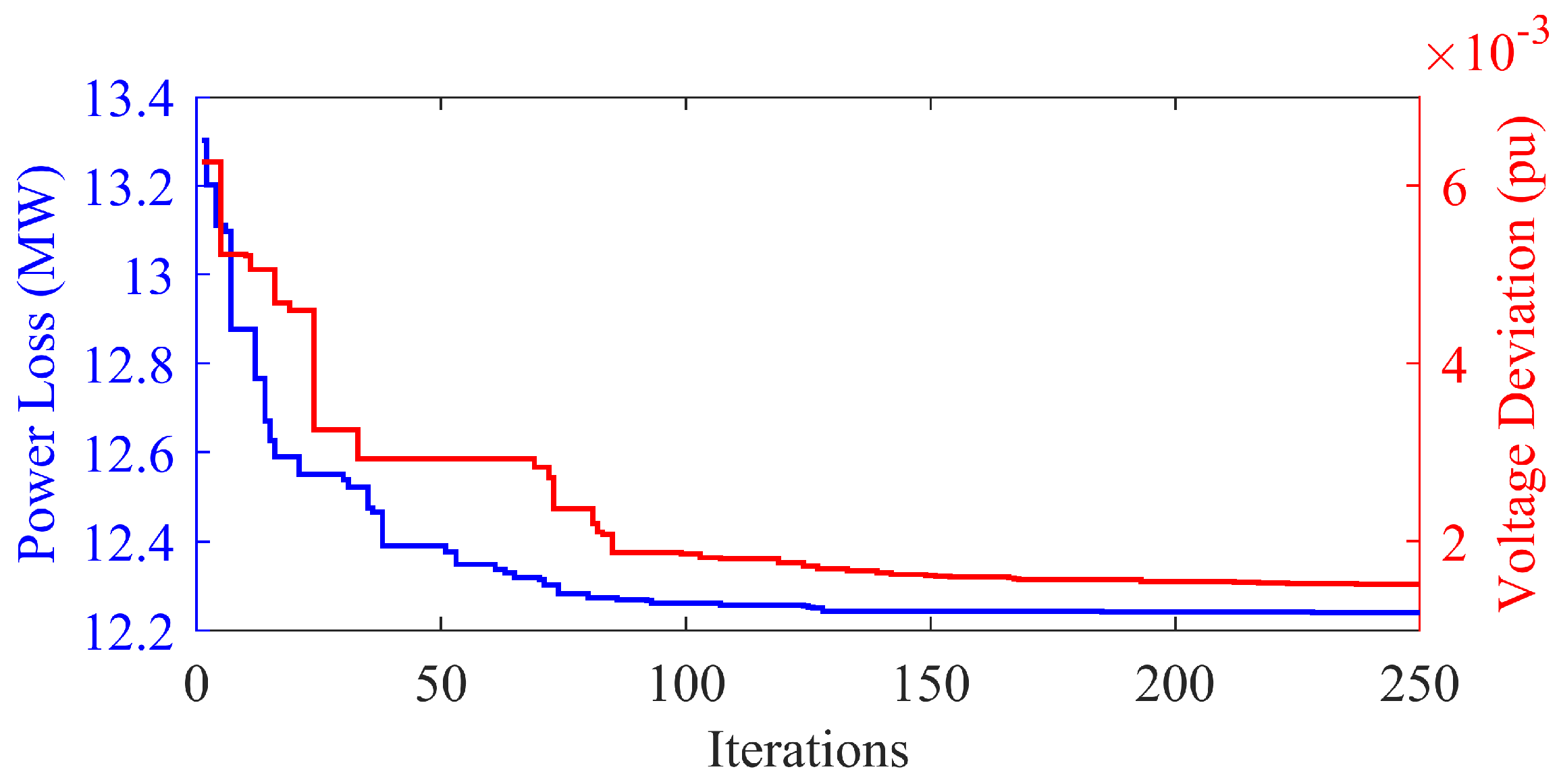
4.3. IEEE 14 Bus Test System Considering Multiobjective Framework

Single objective functions considering $P_{\mathrm{loss}}$ and $V_{\mathrm{dev}}$ were considered independently in previous cases where the objective was to optimally allocate the control variable values to minimize a particular objective individually. In this case, a multiobjective framework [38] to obtain the Pareto optimal solutions, incorporating $P_{\mathrm{loss}}$ and $V_{\mathrm{dev}}$ together, was formulated to solve the multiobjective optimal reactive power dispatch (MO-ORPD) problem. The ORPD problem was addressed using the proposed AHA-based framework that investigated the best settings for the control parameters to obtain the minimum $P_{\mathrm{loss}}$ in the network and the minimum $V_{\mathrm{dev}}$ at the PQ buses simultaneously. The obtained Pareto front is shown in Figure 7, where a compromised optimal solution between the two objectives can be visualized.

4.4. IEEE 14 Bus Test System Considering Integration of Renewable Energy Sources

The IEEE 14 bus test system considered in the previous section for the deterministic study was further utilized for a stochastic-based study by incorporating RES. The resulting test system was regarded as a modified IEEE 14 bus test system wherein 40 MW of maximum capacity for both a PV generator and a wind generator was connected at buses 5 and 8, respectively. The uncertainty in RES and load were considered for the modified IEEE 14 bus test system using the proposed AHA-based framework for the optimization of all scenarios generated in

Table 5. Results of RES-based studied scenarios optimized using the proposed framework.

Scenario	Load	Wind Output	PV Output	${\mathit{\tau }}_{\mathbf{load}}$	${\mathit{\tau }}_{\mathbf{wind}}$	${\mathit{\tau }}_{\mathbf{PV}}$	${\mathit{\tau }}_{\mathit{T}}$	Power Loss (MW)	Expected Power Loss (MW)
1	Off-peak	0	0	0.25	0.073	0.481	0.0088	4.4670	0.0393
2	Off-peak	0	0.485$p_{sr}$	0.25	0.073	0.374	0.0068	3.8289	0.0260
3	Off-peak	0	$p_{sr}$	0.25	0.073	0.145	0.0026	3.3015	0.0086
4	Off-peak	0.47$p_{wr}$	0	0.25	0.76	0.481	0.0914	3.8815	0.3548
5	Off-peak	0.47$p_{wr}$	0.485$p_{sr}$	0.25	0.76	0.374	0.0711	3.4041	0.2420
6	Off-peak	0.47$p_{wr}$	$p_{sr}$	0.25	0.76	0.145	0.0276	3.0444	0.0840
7	Off-peak	$p_{wr}$	0	0.25	0.167	0.481	0.0201	3.7914	0.0762
8	Off-peak	$p_{wr}$	0.485$p_{sr}$	0.25	0.167	0.374	0.0156	3.4671	0.0541
9	Off-peak	$p_{wr}$	$p_{sr}$	0.25	0.167	0.145	0.0061	3.2845	0.0200
10	Mid-peak	0	0	0.7	0.073	0.481	0.0246	5.8392	0.1436
11	Mid-peak	0	0.485$p_{sr}$	0.7	0.073	0.374	0.0191	4.9905	0.0953
12	Mid-peak	0	$p_{sr}$	0.7	0.073	0.145	0.0074	4.2293	0.0313
13	Mid-peak	0.47$p_{wr}$	0	0.7	0.76	0.481	0.2559	4.9863	1.2760
14	Mid-peak	0.47$p_{wr}$	0.485$p_{sr}$	0.7	0.76	0.374	0.199	4.3008	0.8559
15	Mid-peak	0.47$p_{wr}$	$p_{sr}$	0.7	0.76	0.145	0.0771	3.7202	0.2868
16	Mid-peak	$p_{wr}$	0	0.7	0.167	0.481	0.0562	4.6419	0.2609
17	Mid-peak	$p_{wr}$	0.485$p_{sr}$	0.7	0.167	0.374	0.0437	4.1188	0.1800
18	Mid-peak	$p_{wr}$	$p_{sr}$	0.7	0.167	0.145	0.017	3.7169	0.0632
19	On-peak	0	0	0.05	0.073	0.481	0.0018	12.2471	0.0220
20	On-peak	0	0.485$p_{sr}$	0.05	0.073	0.374	0.0014	10.7231	0.0150
21	On-peak	0	$p_{sr}$	0.05	0.073	0.145	0.0005	9.2336	0.0046
22	On-peak	0.47$p_{wr}$	0	0.05	0.76	0.481	0.0183	10.5980	0.1939
23	On-peak	0.47$p_{wr}$	0.485$p_{sr}$	0.05	0.76	0.374	0.0142	9.2524	0.1314
24	On-peak	0.47$p_{wr}$	$p_{sr}$	0.05	0.76	0.145	0.0055	7.9573	0.0438
25	On-peak	$p_{wr}$	0	0.05	0.167	0.481	0.004	9.4285	0.0377
26	On-peak	$p_{wr}$	0.485$p_{sr}$	0.05	0.167	0.374	0.0031	8.2666	0.0256
27	On-peak	$p_{wr}$	$p_{sr}$	0.05	0.167	0.145	0.0012	7.1599	0.0086
Total Expected Power Loss									4.5807

. Twenty-seven scenarios were generated by considering the probabilities of PV, wind and load and a combined RES–load generation probabilities were found as defined by (27), to find the corresponding loss for each scenario. The power loss considering the uncertainties, termed as expected power loss, found for each scenario was given by

$$EP{L}_{TOT}=\sum _{n=1}^{27}EP{L}_n=\sum _{n=1}^{27}{\tau }_{T,n}\times P_{\mathrm{loss},n}$$

(40)

The total expected power loss (TEPL) as obtained from (40) was found to be 4.5807 MW for all scenarios as shown in Table 5.

4.5. IEEE 39 Bus Test System Considering Minimization of $P_{\mathrm{loss}}$

To validate and test the effectiveness of the proposed AHA-based framework, ORPD was further implemented on a medium scale network of the IEEE 39 bus test system. The test system contained five PV buses, three OLTCs and two switchable shunt VAR compensators which were optimized as given in

Table 6. Technical parameters of the IEEE 39 bus test system.

Sr. No.	Parameter	Value
1	Generators	10
2	Branches	46
3	OLTC	5
4	Compensators	6
5	Control variables	21

. The six PV buses were located at buses 1, 2, 3, 6 and 8, three inline OLTCs at branches 4–7, 4–9, and 5–6 and two switchable shunt VAR compensators at buses 9 and 14 in the network. The buses 4, 5, 7, 9, 10, 11, 12, 13 and 14 were PQ buses and were considered to be the candidate buses for the reactive power compensation. The required data including lines interconnection, network data and the system parameters regarding the IEEE 39 bus test system are available in Ref. [39]. The voltages at all the load buses were constrained to remain within the limits of 0.9–1.1 pu at a 100 MVA base. Moreover, the transformer tap positions were restricted between 0.95 and 1.05 pu and the permissible values for the shunt VAR compensators were constrained in the range of 0.9–1.1 pu.

The proposed framework was also validated on the IEEE 39 bus test system to achieve the minimum $P_{\mathrm{loss}}$ as defined by (3). The results for the control variables and power losses with reference to the base case, the AHA and several other well-known optimization techniques implemented in other research studies are compared in

Table 7. Optimal values of control variables with $P_{\mathrm{loss}}$ as an objective function for the IEEE 39 bus test system.

Control Variable	Base Case	BA [14]	CBA-3 [14]	CBA-4 [14]	AHA
$V_{G30}$	1.0499	1.0906	1.0668	1.0810	1.0920
$V_{G31}$	0.9820	1.0999	1.0968	1.0999	1.0993
$V_{G32}$	0.9841	1.0998	1.0989	1.1000	1.0898
$V_{G33}$	0.9972	1.0943	1.0857	1.0952	1.0997
$V_{G34}$	1.0123	1.0956	1.0941	1.0999	1.0972
$V_{G35}$	1.0494	1.1000	1.0976	1.1000	1.0949
$V_{G36}$	1.0636	1.0989	1.1000	1.0992	1.0999
$V_{G37}$	1.0275	1.1000	1.1000	1.1000	1.0996
$V_{G38}$	1.0265	1.0992	1.0988	1.0996	1.0998
$V_{G39}$	1.0300	1.1000	1.1000	1.1000	1.0844
$Q_{C1}$	0	0.1985	0.2392	0.2092	0.01299
$Q_{C5}$	0	0.1266	0.0729	0.1188	0.2353
$Q_{C11}$	0	0.1985	0.2392	0.2092	0.1172
$Q_{C14}$	0	0.1266	0.0729	0.1188	0.2388
$Q_{C22}$	0	0.1985	0.2392	0.2092	0.2883
$Q_{C27}$	0	0.1985	0.2392	0.2092	0.0444
$T_{2-30}$	1.0250	1.0478	1.0591	1.0485	1.0809
$T_{10-32}$	1.0700	1.0700	1.0656	1.0703	1.0868
$T_{12-11}$	1.0060	1.0250	1.0461	1.0337	1.0086
$T_{19-20}$	1.0600	1.0700	1.0645	1.0701	1.0572
$T_{22-35}$	1.0250	1.0034	0.9792	1.0072	1.0867
$P_{\mathrm{loss}}$ (MW)	43.60	36.7317	36.3125	35.9971	35.7699
$V_{\mathrm{dev}}$ (pu)	0.033	0.275	0.271	0.269	0.638

along with the corresponding values of $V_{\mathrm{dev}}$ when $P_{\mathrm{loss}}$ was considered as an objective function. The proposed framework showed a proven ability to attain the minimum losses in the network compared to the base case and other optimization approaches including SFO, GW-PSO and hybrid CBA-4. The losses in the base case were reduced significantly from the value of 43.6 MW to a value of 35.7699 MW found using the proposed framework as is evident from the results. The reduction of 17.7% in losses compared to the base case and a considerable reduction in the percentage from the other optimization approaches proved the effectiveness and robustness of the AHA. This is further represented in Figure 8, where the AHA showed the best results in terms of $P_{\mathrm{loss}}$.

4.6. IEEE 39 Bus Test System Considering Minimization of $V_{\mathrm{dev}}$

Considering $V_{\mathrm{dev}}$ as a second case, the AHA was further utilized for the IEEE 39 bus test system with the objective to achieve minimum voltage deviations as defined by (4). The results for the control variables, voltage deviations and the corresponding power losses were compared with other optimization techniques and are presented in

Table 8. Optimal values of control variables with $V_{\mathrm{dev}}$ as an objective function for the IEEE 39 bus test system.

Control Variable	Base Case	BA	CBA-3	CBA-4	AHA
$V_{G30}$	1.0499	0.9395	1.0286	0.9423	1.022
$V_{G31}$	0.982	1.0999	1.0723	0.9124	1.0438
$V_{G32}$	0.9841	0.9995	0.9782	1.0483	1.018
$V_{G33}$	0.9972	1.069	1.0084	0.9723	1.0016
$V_{G34}$	1.0123	0.9474	0.9797	0.9983	0.9884
$V_{G35}$	1.0494	0.9151	1.0668	0.9011	1.0118
$V_{G36}$	1.0636	0.974	0.9279	0.9866	1.0156
$V_{G37}$	1.0275	0.9001	0.9512	0.9588	0.9006
$V_{G38}$	1.0265	0.9468	0.9362	1.0161	0.9791
$V_{G39}$	1.03	1.0995	1.0077	0.9772	0.981
$Q_{C1}$	0	0.0533	0.2198	0.1234	0.2714
$Q_{C5}$	0	0.1485	0.0554	0.2607	0.2862
$Q_{C11}$	0	0.0533	0.2198	0.1234	0.0365
$Q_{C14}$	0	0.1485	0.0554	0.2607	0.2817
$Q_{C22}$	0	0.0533	0.2198	0.1234	0.143
$Q_{C27}$	0	0.0533	0.2198	0.1234	0.2829
$T_{2-30}$	1.025	0.9563	1.0325	1.0105	1.0201
$T_{10-32}$	1.07	1.0559	0.9972	0.9017	0.9684
$T_{12-11}$	1.006	0.9983	0.9731	0.9318	1.0244
$T_{19-20}$	1.06	0.9124	0.9636	0.9193	0.9893
$T_{22-35}$	1.025	0.9989	0.9457	0.9061	1.0253
$P_{\mathrm{loss}}$ (MW)	43.6	53.74922	53.4682	51.6495	46.96
$V_{\mathrm{dev}}$ (pu)	0.033	0.0825	0.0796	0.0739	0.001

. The AHA-based framework showed a proven ability to attain the minimum $V_{\mathrm{dev}}$ at all the PQ buses in the network compared to the base case and other optimization approaches including SFO, GW-PSO and hybrid CBA-4. The $V_{\mathrm{dev}}$ in the base case was reduced significantly from the value of 0.0330 pu to a value of 0.0011 pu found using the proposed framework. A considerable reduction in $V_{\mathrm{dev}}$ from the base case and the other optimization approaches proved the effectiveness and robustness of the proposed framework. This is further represented in Figure 8, where AHA outperformed the other techniques in terms of $V_{\mathrm{dev}}$. With $V_{\mathrm{dev}}$ as an objective function, the voltages at all the buses in the network approached unity as represented in Figure 9, which was direct evidence for the voltage profile improvement at all the buses in the network.

Convergence curves for the IEEE 39 bus test system considering $P_{\mathrm{loss}}$ and $V_{\mathrm{dev}}$ as an objective function are shown in Figure 10, where the algorithm reached the optimal solution in 130 iterations and 230 iterations, respectively. The maximum number of iterations for the algorithm was set to 250. The fast convergence rate of the AHA compared to other optimization algorithms showed its better performance and effectiveness. The execution time of the AHA for the IEEE 39 bus test system was found to be equal to 139 s.

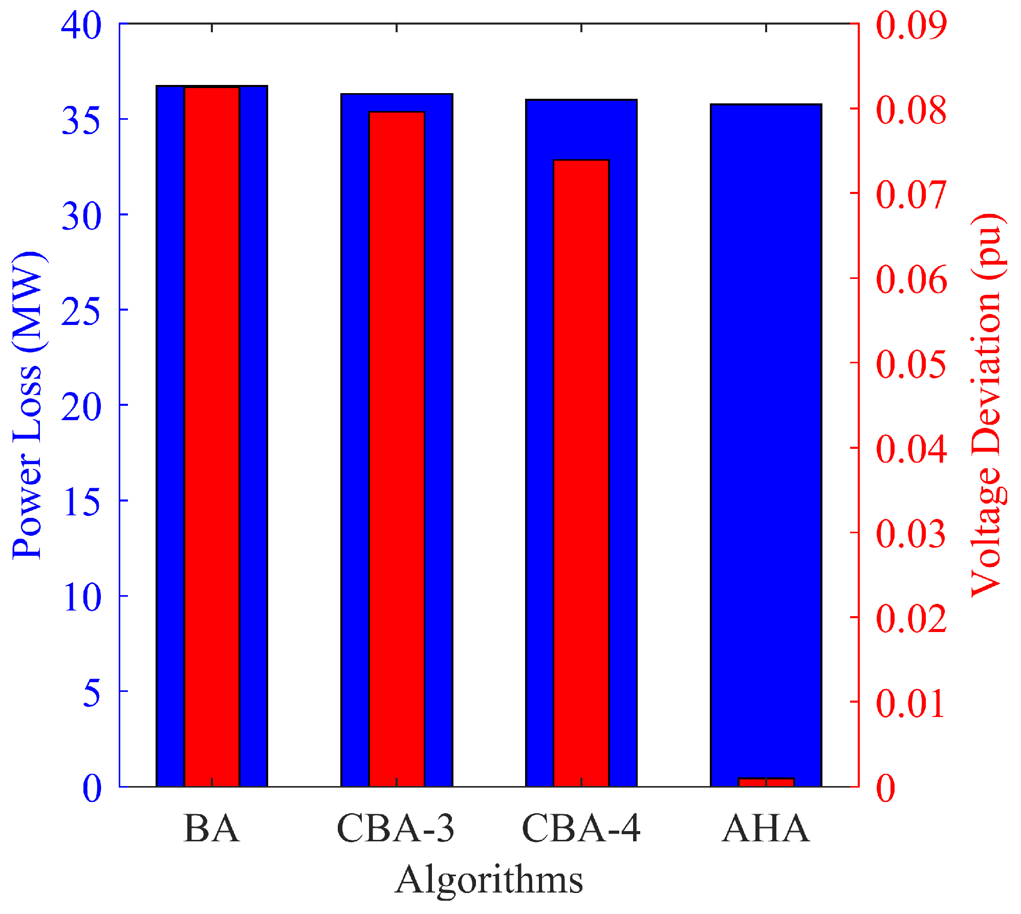
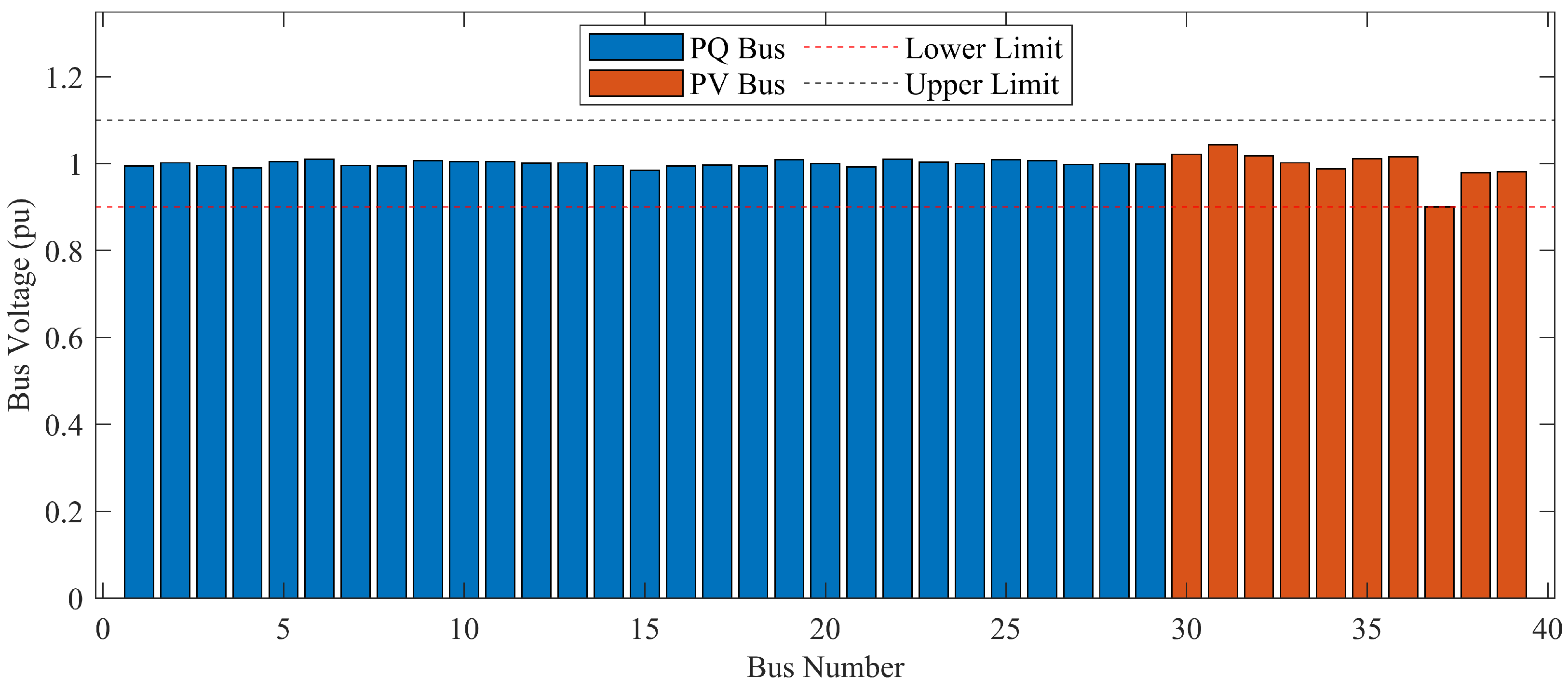
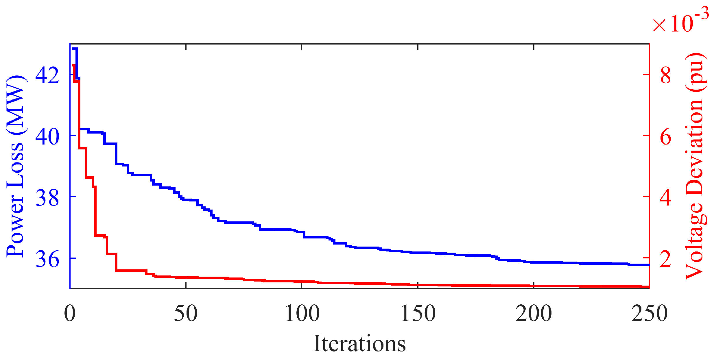
4.7. IEEE 39 Bus Test System Considering Multiobjective Framework

A multiobjective framework [38] to obtain the Pareto optimal solutions, incorporating $P_{\mathrm{loss}}$ and $V_{\mathrm{dev}}$ together, was formulated to solve the multiobjective optimal reactive power dispatch (MO-ORPD) problem. The ORPD problem was addressed using the proposed AHA-based framework that investigated the best settings for the control parameters to obtain the minimum $P_{\mathrm{loss}}$ in the network and minimum $V_{\mathrm{dev}}$ at the PQ buses simultaneously. The obtained Pareto front is shown in Figure 11, where a compromise optimal solution between the two objectives can be visualized. The optimal $P_{\mathrm{loss}}$ was found to be 39.73 MW with the corresponding optimal $V_{\mathrm{dev}}$ equal to 0.08056 pu.

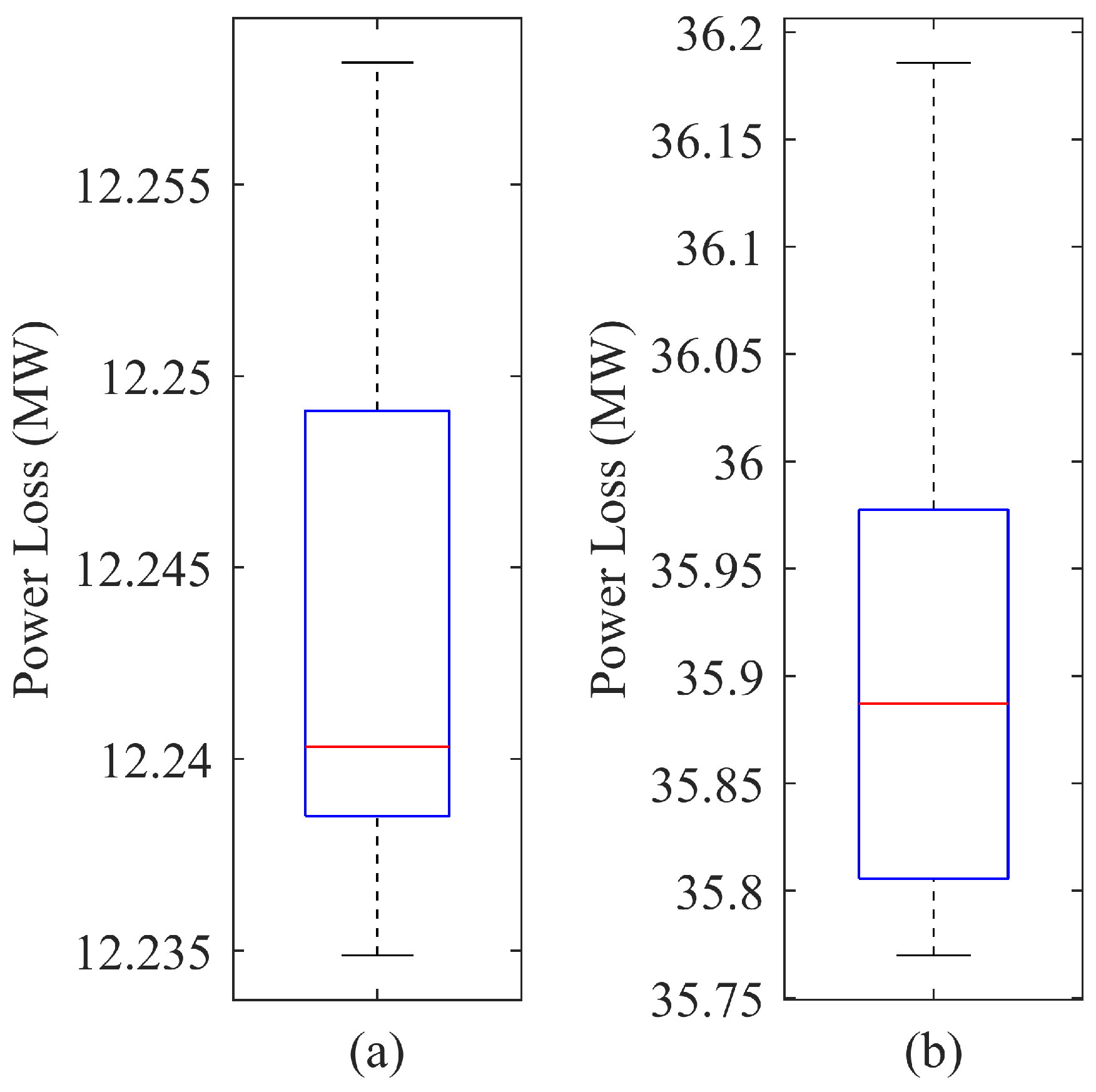
4.8. Statistical Significance of ORPD Results

The validity and verification of the best ORPD solution situated in the vicinity of the optimal solution were considered through the boxplots [38] shown in Figure 12. The minimum $P_{\mathrm{loss}}$ was ensured by taking 30 independent test runs of the proposed framework for the IEEE 14 bus test system and IEEE 39 bus test system cases. The data of the 30 test runs were taken for the boxplots presented in Figure 12 for the two test systems. It is apparent from the boxplots that there were no outliers in the IEEE 14 and 39 bus test system results. The best solutions were found to be in close proximity to the global optima.

A further validation of the ORPD results optimized by the proposed AHA-based framework for the IEEE 14 bus test system and the IEEE 39 bus test system was carried out and the significance of the results were found in terms of p-values. In the ORPD problem, $P_{\mathrm{loss}}$ for 30 iterations was designated as a dependent variable whereas the voltages at PV buses, VAR compensators and OLTCs were regarded as decision variables. The decision variables directly influenced the dependent variable, and the model was implemented in SPSS (Statistical Package for the Social Sciences) software. A linear regression was performed using SPSS and a p-value test was also run on the estimated coefficients of the model. The statistical results were obtained for the IEEE 14 bus test system and the IEEE 39 bus test system and are listed in

Table 9. Statistical significance of multiple tests runs for the IEEE 14 bus test system optimized by the proposed framework.

Decision Variables	Beta	Sig.	Decision Variables	Beta	Sig.
$V_{G1}$	−0.022	0.422	$Q_{C9}$	−0.1	0.173
$V_{G2}$	0.036	0.182	$Q_{C14}$	0.02	0.474
$V_{G3}$	−0.064	0.017	$T_{4-7}$	0.31	0.024
$V_{G6}$	−0.048	0.624	$T_{4-9}$	0.457	0.052
$V_{G8}$	−0.155	0.195	$T_{5-6}$	−0.1	0.173

and

Table 10. Statistical significance of multiple tests runs for the IEEE 39 bus test system optimized by the proposed framework.

Decision Variables	Beta	Sig.	Decision Variables	Beta	Sig.
$V_{G30}$	−0.342	0.005	$Q_{C5}$	−0.185	0.115
$V_{G31}$	0.005	0.963	$Q_{C11}$	0.199	0.163
$V_{G32}$	−0.156	0.206	$Q_{C14}$	−0.008	0.941
$V_{G33}$	−0.345	0.007	$Q_{C22}$	0.05	0.649
$V_{G34}$	−0.295	0.155	$Q_{C27}$	−0.02	0.877
$V_{G35}$	−0.067	0.516	$T_{2-30}$	−0.195	0.117
$V_{G36}$	−0.199	0.135	$T_{10-32}$	−0.225	0.035
$V_{G37}$	−0.257	0.061	$T_{12-11}$	−0.113	0.262
$V_{G38}$	−0.074	0.458	$T_{19-20}$	−0.245	0.274
$V_{G39}$	−0.127	0.233	$T_{22-35}$	−0.248	0.033
$Q_{C1}$	−0.139	0.16

, respectively. From the results, the p-values for the IEEE 14 bus test system, variables $V_{G3}$, $T_{4-7}$, $T_{4-9}$ and $T_{5-6}$ showed a significant effect on the solution and their p-values for the estimated coefficients were less than 0.1, i.e., the results were statistically significant at the 90% level and met the confidence interval of 5%. The p-value test for the IEEE 39 bus test system showed that the variables $V_{G30}$, $V_{G33}$, $V_{G37}$, $Q_{C-5}$, $T_{2-30}$, $T_{10-32}$ and $T_{22-35}$ had a significant effect on the solution and their p-values for the estimated coefficients were also less than 0.1, i.e., the results were statistically significant at the 90% level and met the confidence interval of 10%.

The boxplots and the p-values confirmed the performance of the ORPD problem with the proposed framework. The proposed framework converged to the optimal solution in terms of $P_{\mathrm{loss}}$ and $V_{\mathrm{dev}}$.

The best (minimum), worst (maximum) and average (mean) values of the control variables for the IEEE 14 and IEEE 39 bus test systems were compared with other techniques in

Table 11. Statistical tests on the IEEE 14 and 39 bus test systems for cases 1 and 2 optimized by the proposed AHA-based framework.

IEEE 14 Bus Test System
Algorithm	Best (MW)	Worst (MW)	Average (MW)	SD
DEEP [40]	12.4489	12.4507	12.4494	0.0005
CSSP4 [41]	12.4087	12.4974	12.4393	0.228
DE [42]	12.4486	12.4496	12.4486	0.0018
CBA-4	12.2923	12.3098	12.3042	0.0046
AHA	12.2349	12.2667	12.2443	0.0079
Algorithm	Best (${\mathit{V}}_{\mathrm{dev}}$)	Worst (${\mathit{V}}_{\mathrm{dev}}$)	Average (${\mathit{V}}_{\mathrm{dev}}$)	SD
IGSA-CSS [17]	0.0339	0.0906	0.0458	0.017
GWO-PSO	0.2133	-	-	-
BA	0.0336	0.0515	0.041	0.0058
CBA-4	0.033	0.0489	0.0368	0.0029
AHA	0.0015	0.0039	0.0037	0.0004
IEEE 39 Bus Test System
Algorithm	Best (MW)	Worst (MW)	Average (MW)	SD
GWO-PSO	41.8892	-	-	-
CBA-3	36.3125	37.7435	36.4527	0.3272
CBA-4	35.9971	36.6986	36.1028	0.2122
AHA	35.7699	36.1857	35.9044	0.1098
Algorithm	Best (${\mathit{V}}_{\mathrm{dev}}$)	Worst (${\mathit{V}}_{\mathrm{dev}}$)	Average (${\mathit{V}}_{\mathrm{dev}}$)	SD
BA	0.0825	-	-	-
CBA-3	0.0796	0.0921	0.0846	0.0034
CBA-4	0.0739	0.0864	0.0763	0.0027
AHA	0.001	0.0013	0.0011	5.0083

. Moreover, the standard deviation (SD) of 20 independent runs was calculated. These statistical results clearly manifested the performance and supremacy of the AHA compared to other previously proposed techniques.

5. Conclusions

This research work presented a holistic analysis on a multiobjective framework considering one of the latest optimization algorithms, the AHA, that was investigated and implemented to solve the ORPD problem with and without the inclusion of RES. A scenario-based modeling of PV, wind and load was presented to cater to the intermittency and uncertainty in RES and loads. Three objective functions including a multiobjective framework (MO-ORPD) considering the set of equality and nonequality constraints were considered to minimize the active power losses and to ameliorate the voltage profile at all the load buses in the network. The proposed AHA-based framework was tested and validated on standard IEEE 14 and 39 bus test systems, and the acquired results were compared with various optimization techniques, namely, SFO, GWO-PSO, SCA and CBA-4. The proposed AHA-based framework outperformed its competitors in terms of active power loss minimization and total voltage deviation minimization, with a fast convergence rate and less computational time. Further, the proposed framework was also found effective in providing desirable solutions in terms of the average, best, worst and SD indices. Boxplots were created and statistical tests were performed using SPSS to justify the effectiveness of the proposed framework. As a result of the statistical analysis, the said algorithm can be considered as an effective optimization tool for power system control centers to make optimal dispatch decisions, while confronting the ORPD problem. The optimal location of the reactive VAR sources and FACTS devices is also planned for the future work.

References

1. Seifi, H.; Sepasian, M.S. Electric Power System Planning: Issues, Algorithms and Solutions; Springer: Berlin/Heidelberg, Germany, 2011; Volume 49. [Google Scholar]
2. AlRashidi, M.; El-Hawary, M. Applications of computational intelligence techniques for solving the revived optimal power flow problem. Electr. Power Syst. Res. 2009, 79, 694–702. [Google Scholar] [CrossRef]
3. Balu, K.; Mukherjee, V. Optimal siting and sizing of distributed generation in radial distribution system using a novel student psychology-based optimization algorithm. Neural Comput. Appl. 2021, 33, 15639–15667. [Google Scholar] [CrossRef]
4. Yuvaraj, T.; Devabalaji, K.; Srinivasan, S.; Prabaharan, N.; Hariharan, R.; Alhelou, H.H.; Ashokkumar, B. Comparative analysis of various compensating devices in energy trading radial distribution system for voltage regulation and loss mitigation using Blockchain technology and Bat Algorithm. Energy Rep. 2021, 7, 8312–8321. [Google Scholar] [CrossRef]
5. Saddique, M.S.; Bhatti, A.R.; Haroon, S.S.; Sattar, M.K.; Amin, S.; Sajjad, I.A.; ul Haq, S.S.; Awan, A.B.; Rasheed, N. Solution to optimal reactive power dispatch in transmission system using meta-heuristic techniques―Status and technological review. Electr. Power Syst. Res. 2020, 178, 106031. [Google Scholar] [CrossRef]
6. Lee, K.Y.; Yang, F.F. Optimal reactive power planning using evolutionary algorithms: A comparative study for evolutionary programming, evolutionary strategy, genetic algorithm, and linear programming. IEEE Trans. Power Syst. 1998, 13, 101–108. [Google Scholar] [CrossRef]
7. Quintana, V.; Santos-Nieto, M. Reactive-power dispatch by successive quadratic programming. IEEE Trans. Energy Convers. 1989, 4, 425–435. [Google Scholar] [CrossRef]
8. Wu, Q.H.; Ma, J. Power system optimal reactive power dispatch using evolutionary programming. IEEE Trans. Power Syst. 1995, 10, 1243–1249. [Google Scholar] [CrossRef]
9. Manasvi, K.; Venkateswararao, B.; Devarapalli, R.; Prasad, U. PSO Based Optimal Reactive Power Dispatch for the Enrichment of Power System Performance. In Recent Advances in Power Systems; Springer: Berlin/Heidelberg, Germany, 2021; pp. 267–276. [Google Scholar]
10. Saddique, M.S.; Habib, S.; Haroon, S.S.; Bhatti, A.R.; Amin, S.; Ahmed, E.M. Optimal Solution of Reactive Power Dispatch in Transmission System to Minimize Power Losses using Sine-Cosine Algorithm. IEEE Access 2022, 10, 20223–20239. [Google Scholar] [CrossRef]
11. Shanono, I.H.; Muhammad, A.; Abdullah, N.R.H.; Daniyal, H.; Tiong, M.C. Optimal reactive power dispatch: A bibliometric analysis. J. Electr. Syst. Inf. Technol. 2021, 8, 1–23. [Google Scholar] [CrossRef]
12. Roy, R.; Das, T.; Mandal, K.K. Optimal reactive power dispatch using a novel optimization algorithm. J. Electr. Syst. Inf. Technol. 2021, 8, 1–24. [Google Scholar] [CrossRef]
13. Abdel-Fatah, S.; Ebeed, M.; Kamel, S. Optimal reactive power dispatch using modified sine cosine algorithm. In Proceedings of the 2019 International Conference on Innovative Trends in Computer Engineering (ITCE, Aswan, Egypt, 2–4 February 2019; pp. 510–514. [Google Scholar]
14. Mugemanyi, S.; Qu, Z.; Rugema, F.X.; Dong, Y.; Bananeza, C.; Wang, L. Optimal reactive power dispatch using chaotic bat algorithm. IEEE Access 2020, 8, 65830–65867. [Google Scholar] [CrossRef]
15. Najafi, A.; Falaghi, H. Optimal reactive power dispatch using teaching learning based optimization algorithm in the presence of wind turbine uncertainty. Iran. Electr. Ind. J. Qual. Product. 2018, 7, 93–101. [Google Scholar]
16. Reddy, S.S. Optimal Reactive Power Scheduling Using Cuckoo Search Algorithm. Int. J. Electr. Comput. Eng. 2017, 7, 2349–2356. [Google Scholar]
17. Chen, G.; Liu, L.; Zhang, Z.; Huang, S. Optimal reactive power dispatch by improved GSA-based algorithm with the novel strategies to handle constraints. Appl. Soft Comput. 2017, 50, 58–70. [Google Scholar] [CrossRef]
18. Shaheen, M.A.; Hasanien, H.M.; Alkuhayli, A. A novel hybrid GWO-PSO optimization technique for optimal reactive power dispatch problem solution. Ain Shams Eng. J. 2021, 12, 621–630. [Google Scholar] [CrossRef]
19. Khan, N.H.; Wang, Y.; Tian, D.; Jamal, R.; Ebeed, M.; Deng, Q. Fractional PSOGSA algorithm approach to solve optimal reactive power dispatch problems with uncertainty of renewable energy resources. IEEE Access 2020, 8, 215399–215413. [Google Scholar] [CrossRef]
20. Aljohani, T.M.; Ebrahim, A.F.; Mohammed, O. Single and multiobjective optimal reactive power dispatch based on hybrid artificial physics–particle swarm optimization. Energies 2019, 12, 2333. [Google Scholar] [CrossRef] [Green Version]
21. Wei, Y.; Zhou, Y.; Luo, Q.; Deng, W. Optimal reactive power dispatch using an improved slime mould algorithm. Energy Rep. 2021, 7, 8742–8759. [Google Scholar] [CrossRef]
22. Abd-El Wahab, A.M.; Kamel, S.; Hassan, M.H.; Mosaad, M.I.; AbdulFattah, T.A. Optimal Reactive Power Dispatch Using a Chaotic Turbulent Flow of Water-Based Optimization Algorithm. Mathematics 2022, 10, 346. [Google Scholar] [CrossRef]
23. Naderi, E.; Narimani, H.; Pourakbari-Kasmaei, M.; Cerna, F.V.; Marzband, M.; Lehtonen, M. State-of-the-art of optimal active and reactive power flow: A comprehensive review from various standpoints. Processes 2021, 9, 1319. [Google Scholar] [CrossRef]
24. Sánchez-Mora, M.M.; Bernal-Romero, D.L.; Montoya, O.D.; Villa-Acevedo, W.M.; López-Lezama, J.M. Solving the Optimal Reactive Power Dispatch Problem through a Python-DIgSILENT Interface. Computation 2022, 10, 128. [Google Scholar] [CrossRef]
25. Zhou, B.; Shen, X.; Pan, C.; Bai, Y.; Wu, T. Optimal Reactive Power Dispatch under Transmission and Distribution Coordination Based on an Accelerated Augmented Lagrangian Algorithm. Energies 2022, 15, 3867. [Google Scholar] [CrossRef]
26. Morán-Burgos, J.A.; Sierra-Aguilar, J.E.; Villa-Acevedo, W.M.; López-Lezama, J.M. A Multi-Period Optimal Reactive Power Dispatch Approach Considering Multiple Operative Goals. Appl. Sci. 2021, 11, 8535. [Google Scholar] [CrossRef]
27. Ashraf, M.M.; Malik, T.N. Least cost generation expansion planning in the presence of renewable energy sources using correction matrix method with indicators-based discrete water cycle algorithm. J. Renew. Sustain. Energy 2019, 11, 056301. [Google Scholar] [CrossRef]
28. Nawaz, U.; Malik, T.N.; Ashraf, M.M. Least-cost generation expansion planning using whale optimization algorithm incorporating emission reduction and renewable energy sources. Int. Trans. Electr. Energy Syst. 2020, 30, e12238. [Google Scholar] [CrossRef]
29. Abbas, T.; Ashraf, M.M.; Malik, T.N. Least Cost Generation Expansion Planning considering Renewable Energy Resources Using Sine Cosine Algorithm. Arab. J. Sci. Eng. 2022, 1–19. [Google Scholar] [CrossRef]
30. ElSayed, S.K.; Elattar, E.E. Slime Mold Algorithm for Optimal Reactive Power Dispatch Combining with Renewable Energy Sources. Sustainability 2021, 13, 5831. [Google Scholar] [CrossRef]
31. Ashraf, M.M.; Malik, T.N. A Novel Optimization Framework for the Least Cost Generation Expansion Planning in the Presence of Renewable Energy Sources considering Regional Connectivity. Arab. J. Sci. Eng. 2020, 45, 6423–6451. [Google Scholar] [CrossRef]
32. Ashraf, M.M.; Malik, T.N. A hybrid teaching–learning-based optimizer with novel radix-5 mapping procedure for minimum cost power generation planning considering renewable energy sources and reducing emission. Electr. Eng. 2020, 102, 2567–2582. [Google Scholar] [CrossRef]
33. Ebeed, M.; Alhejji, A.; Kamel, S.; Jurado, F. Solving the optimal reactive power dispatch using marine predators algorithm considering the uncertainties in load and wind-solar generation systems. Energies 2020, 13, 4316. [Google Scholar] [CrossRef]
34. Naidji, M.; Boudour, M. Stochastic multi-objective optimal reactive power dispatch considering load and renewable energy sources uncertainties: A case study of the Adrar isolated power system. Int. Trans. Electr. Energy Syst. 2020, 30, e12374. [Google Scholar] [CrossRef]
35. Zhao, W.; Wang, L.; Mirjalili, S. Artificial hummingbird algorithm: A new bio-inspired optimizer with its engineering applications. Comput. Methods Appl. Mech. Eng. 2022, 388, 114194. [Google Scholar] [CrossRef]
36. Zhao, W.; Zhang, Z.; Mirjalili, S.; Wang, L.; Khodadadi, N.; Mirjalili, S.M. An effective multi-objective artificial hummingbird algorithm with dynamic elimination-based crowding distance for solving engineering design problems. Comput. Methods Appl. Mech. Eng. 2022, 398, 115223. [Google Scholar] [CrossRef]
37. Saadat, H. Power System Analysis; McGraw-Hill: New York, NY, USA, 1999. [Google Scholar]
38. Rice, J.A. Mathematical Statistics and Data Analysis; Brooks/Cole ISE: Bonn, Germany, 2006. [Google Scholar]
39. Athay, T.; Podmore, R.; Virmani, S. A practical method for the direct analysis of transient stability. IEEE Trans. Power Appar. Syst. 1979, PAS-98, 573–584. [Google Scholar] [CrossRef]
40. Chung, C.; Liang, C.; Wong, K.; Duan, X. Hybrid algorithm of differential evolution and evolutionary programming for optimal reactive power flow. IET Gener. Transm. Distrib. 2010, 4, 84–93. [Google Scholar] [CrossRef]
41. Liang, C.; Chung, C.; Wong, K.; Duan, X. Comparison and improvement of evolutionary programming techniques for power system optimal reactive power flow. IEEE Proc.-Gener. Transm. Distrib. 2006, 153, 228–236. [Google Scholar] [CrossRef]
42. Liang, C.; Chung, C.; Wong, K.; Duan, X.; Tse, C. Study of differential evolution for optimal reactive power flow. IET Gener. Transm. Distrib. 2007, 1, 253–260. [Google Scholar] [CrossRef]
Figure 1. Mapping procedure for control variable of ORPD problem.
Energies 15 09250 g001
Figure 2. Schematic flowchart of AHA.
Energies 15 09250 g002
Figure 3. Schematic flowchart of the proposed AHA-based framework to optimize the ORPD problem.
Energies 15 09250 g003
Figure 4. Comparison of P loss and V dev for IEEE 14 bus test system optimized using the proposed framework.
Energies 15 09250 g004
Figure 5. Bus voltages of the IEEE 14 bus test system.
Energies 15 09250 g005
Figure 6. Convergence curves of P loss and V dev for the IEEE 14 bus test system optimized using the proposed framework.
Energies 15 09250 g006
Figure 7. IEEE 14 bus test system: a multiobjective approach based on Pareto optimal solutions.
Energies 15 09250 g007
Figure 8. Comparison of P loss and V dev for the IEEE 39 bus test system optimized using the proposed framework.
Energies 15 09250 g008
Figure 9. Bus voltages of the IEEE 39 bus power system.
Energies 15 09250 g009
Figure 10. Convergence curves of P loss and V dev for the IEEE 39 bus test system optimized using the proposed framework.
Energies 15 09250 g010
Figure 11. IEEE 39 bus test system: a multiobjective approach based on Pareto optimal solutions.
Energies 15 09250 g011
Figure 12. Validity of best ORPD results using proposed AHA-based framework: (a) IEEE 14 bus test system, (b) IEEE 39 bus test system.
Energies 15 09250 g012