Numerical Modeling of Shell-and-Tube-like Elastocaloric Regenerator

Abstract

Elastocaloric cooling is considered an environmentally friendly future alternative to vapor-compression technology. Recently, a shell-and-tube-like elastocaloric regenerator loaded in compression has demonstrated record-breaking heat-pumping performance and fatigue-resistant operation. The aim of this work is thus to present a new 1D numerical model to simulate and optimize the operation of an elastocaloric regenerator with a shell-and-tube-like design. In the first part of this work, the superelastic and elastocaloric properties of a single NiTi tube, which serve as input data for the numerical model, were determined through experimental characterization and phenomenological modeling. In the second part, the results of the numerical model were compared with the experimentally obtained results. Relatively good agreement was found regarding the temperature span, cooling and heating power, and COP values, which indicates that the developed numerical model could be used for accurate optimization of shell-and-tube-like elastocaloric regenerators. Finally, the effects of operating conditions and hysteresis losses on the performance of the shell-and-tube-like elastocaloric regenerator are modeled and discussed. This work shows that the shell-and-tube-like elastocaloric regenerator with this configuration can achieve a maximum temperature span of more than 50 K at zero-thermal-load conditions and a maximum cooling/heating power of up to 4000 W·kg⁻¹ and COP of about 4 (at zero temperature span).

1. Introduction

Growing global cooling demand and environmental awareness have led to the abandonment of environmentally harmful refrigerants such as chlorofluorocarbons (CFCs) and hydrofluorocarbons (HFCs), which have been widely used in vapor-compression technology [1]. In the long term, they must be replaced by natural refrigerants, such as hydrocarbons (HCs) and carbon dioxide (CO₂). However, these are not faultless since all HCs are at least slightly flammable, and CO₂ has rather low efficiency in hot climates [2,3]. Moreover, large vapor-compression systems achieve relatively high exergy efficiencies (>50%), but this is not true for small systems, which are characterized by relatively low exergy efficiencies (<30%) [4,5]. Due to the rapid progress of developing countries and global warming trends, the number of small refrigeration and especially air-conditioning systems is expected to increase significantly over the next two decades. Elastocaloric cooling is considered a promising alternative to vapor-compression technology used for cooling/heating, and its development could provide a solution for environmentally friendly cooling and heat-pumping systems [6]. It has two important advantages over vapor-compression technology: it is environmentally benign during operation and can potentially achieve better efficiency (especially compared to small refrigeration units). In 2014 and 2016, the US Department of Energy [7] and the European Commission [8], respectively, recognized elastocaloric cooling as the most promising future non-vapor-compression refrigeration technology. In addition to traditional HVAC applications, elastocaloric cooling can play an important role in micro-cooling applications for thermal management of electronic devices [9,10], such as batteries and supercapacitors [11,12].

Elastocaloric technology is based on the elastocaloric effect (eCE) that occurs in superelastic shape memory alloys (and other shape memory materials) [13]. Although eCE has been known for more than 40 years [14], it is only in the last two decades that it has attracted the attention of the scientific community in the field of refrigeration [15,16]. The application of sufficient mechanical stress to a superelastic shape memory alloy (SMA) causes the transformation of the crystal lattice from the high-temperature austenite phase (cubic—B2) to the low-temperature martensite phase (less ordered monoclinic—B19 prime), which is called forward martensitic transformation. This is an exothermic process that causes a temperature increase of SMA under adiabatic conditions or an entropy decrease under isothermal conditions. Namely, under adiabatic conditions, which is the case of rapid mechanical loading, the latent heat of transformation does not have time to be transferred to the surroundings, so the elastocaloric material heats up. In contrast, under isothermal conditions, which occur during slow mechanical loading, the latent heat is transferred to the surroundings and the temperature of the material remains constant. The reverse martensitic transformation, which is endothermic, occurs when the mechanical stress is removed and causes a temperature decrease under adiabatic conditions or entropy increase under isothermal conditions. The temperature and entropy changes associated with the phase transformation can be used for cooling or heat-pumping if used in the caloric cooling cycle. The basic thermodynamic cycle for caloric technologies is the Brayton cycle, which is based on the following four operational steps. The first step is the adiabatic mechanical loading of the elastocaloric material (e.g., superelastic SMA), which causes the eCE and thus the temperature rise of the elastocaloric material (eCM), followed by the heat transfer to the surroundings at constant (high) stress/strain in the second step. The third step is the adiabatic unloading of the eCM, causing the eCM to cool below the initial temperature. The last step is heat transfer from the surroundings to the eCM at constant (low) stress/strain. If these four steps are repeated continuously, active cooling or heating can be achieved. A graphical presentation of the eCE is shown in Figure S1 in the Supplementary materials. Among the many eCMs known today, NiTi alloys are the most studied eCMs, because they are commercially available, have a large latent heat, and have relatively good fatigue life compared to other eCMs. The use of alloying elements such as Cu, Fe, V, and Co has been shown to reduce hysteresis losses and improve the fatigue life of NiTi-based alloys, but at the expense of lower eCE [17,18,19,20]. In addition to NiTi-based alloys, eCE has also been studied in Cu-based [21,22], Fe-based [23], and magnetic shape memory alloys [24,25] as well as in shape memory polymers [26,27]. Recent reviews on eCMs can be found in [13,28,29,30].

To date, about 15 proof-of-the-concept elastocaloric devices have been developed and tested. Their operating principles and performances can be found in the literature [31,32,33,34,35,36,37,38,39,40]. The best overall cooling and heat-pumping performance to date has been achieved by shell-and-tube-like active elastocaloric regenerator (AeCR) based on NiTi tubes, which generated a maximum temperature span of 31.3 K (in heat-pumping mode) and more than 60 W of cooling and heating power (4400 W·kg⁻¹ of eCM) [35]. The concept of active regeneration was originally developed in the field of magnetocaloric cooling [41] and was later applied also in other caloric technologies [31,42]. An active elastocaloric regenerator (AeCR) is essentially a porous structure (matrix) made of eCM through which a heat transfer fluid (HTF), such as water, oscillates between the heat sink and the heat source. The eCM in the AeCR has a dual function, acting as both a refrigerant and a heat regenerator enabling an increase in the temperature span. The active regenerative caloric cycle is a unique thermodynamic cycle in which a temperature profile is established along the length of the regenerator under steady-state conditions. Therefore, each part of the caloric material undergoes its own thermodynamic cycle at different temperatures, so the temperature span between the heat source and the heat sink can be larger than the adiabatic temperature change of the eCM itself.

In parallel with the development of elastocaloric devices, several numerical models have been developed in recent years to simulate and optimize their operation. Among the developed models, a distinction can be made between steady-state and transient models, the latter being further divided into one-dimensional (1D) and two-dimensional (2D) models. The steady-state models are based on simple energy balance equations and use certain performance metrics as input data [43,44]. This approach is usually used for simulating complex systems to gain insight into the overall process behavior without much computational effort. In more complex transient models, governing differential equations are used to describe the thermal state of an elastocaloric device. Most transient numerical models for elastocaloric devices are 1D. Although 2D models can be more accurate, 1D models represent a good compromise between the complexity, the computational time required, and the accuracy of the results. The transient numerical models are usually based on a set of coupled governing differential equations describing the thermal state of the elastocaloric porous matrix and the HTF (if included). These models can be divided into the numerical models of elastocaloric devices with the heat-recovery principle [45,46], the active regeneration principle [47,48,49,50,51,52,53,54,55,56], the single-stage principle [32,57] and the elastocaloric heat-pipe principle [58].

The developed models of elastocaloric devices can be further distinguished with respect to the implementation of eCE. Some models (e.g., [9,50]) integrate measured values of adiabatic temperature changes directly into the governing equation of the eCM. However, since eCE depends on the applied stress/strain and temperature, a more advanced characterization of eCE is usually required to correctly capture the elastocaloric response of the eCM in the model. Since eCE is closely related to the superelasticity of SMA, it can be calculated based on the superelastic behavior as a function of stress/strain and temperature. Tušek et al. [47] presented the phenomenological model describing the superelastic and moreover the elastocaloric properties calculated based on the Maxwell relation assuming complete phase transformation. Qian et al. [54] used a superelastic model that takes into account the kinetics of phase transformation and allows accurate prediction of eCE under partial phase transformation. This model is based on the Müller-Achenbach-Seelecke model [59], which considers martensite and austenite fractions during transformation. A similar approach was also used in [32,45,46,52,53,55,56,60]. Recently, Bachmann et al. [61] modified the material modeling approach of the magnetocaloric effect presented by Hess et al. [62] and used it for modeling the eCE. It is based on phenomenological modeling of heat capacity as a function of temperature and stress, based on which the isothermal entropy change, adiabatic temperature change, and strain of the eCM were calculated. Griffith et al. [63] recently presented a model for predicting the thermal behavior of eCM based on the Debye approximation [64].

Here, we present a new, first-of-its-kind numerical model to simulate and optimize the cooling and heating performance of the shell-and-tube-like AeCR. As recently shown [35], such a design of the AeCR shows fatigue-resistant operation (due to compressive loading) and has the best overall specific cooling/heating performance of all elastocaloric devices developed to date. The developed numerical model is based on the governing differential equations describing the thermal state of the regenerator. These were previously presented by Ahčin et al. [65] for a passive oscillating-flow shell-and-tube-like regenerator to characterize their thermohydraulic properties. In this work, the model is extended to include the elastocaloric properties of the NiTi tube obtained through experimental characterization and phenomenological modeling. The eCE is implemented in a unique way that allows us to model partial transformations, including hysteresis losses without compromising computational efficiency. The numerical model is verified using the experimentally determined cooling and heat-pumping properties of the shell-and-tube-like AeCR at different operating conditions (see [35] for details on the experimental results). Finally, the influence of the operating conditions (applied strain, operating frequency, displaced fluid volume ratio, and temperature span) and hysteresis losses on the cooling and heat-pumping performance is modeled and discussed.

The rest of the paper is organized as follows. In Section 2, the methods are presented, where we describe the experimental determination and phenomenological modeling of the superelastic and elastocaloric properties, as well as the numerical modeling of the active elastocaloric regenerator. In Section 3, the main results of this work are shown, where we present a verification of the numerical model against the experimental results and the influence of some of the most important operating parameters on the regenerator’s performance. In Section 4, the main conclusions of this work are drawn.

2. Methods

In the first part of this work, the superelastic and elastocaloric properties of the NiTi tube were determined by experimental characterization. The obtained experimental data were then used as input data for the phenomenological model, based on which a set of elastocaloric properties was calculated as a function of applied strain and temperature, necessary for further AeCR modeling.

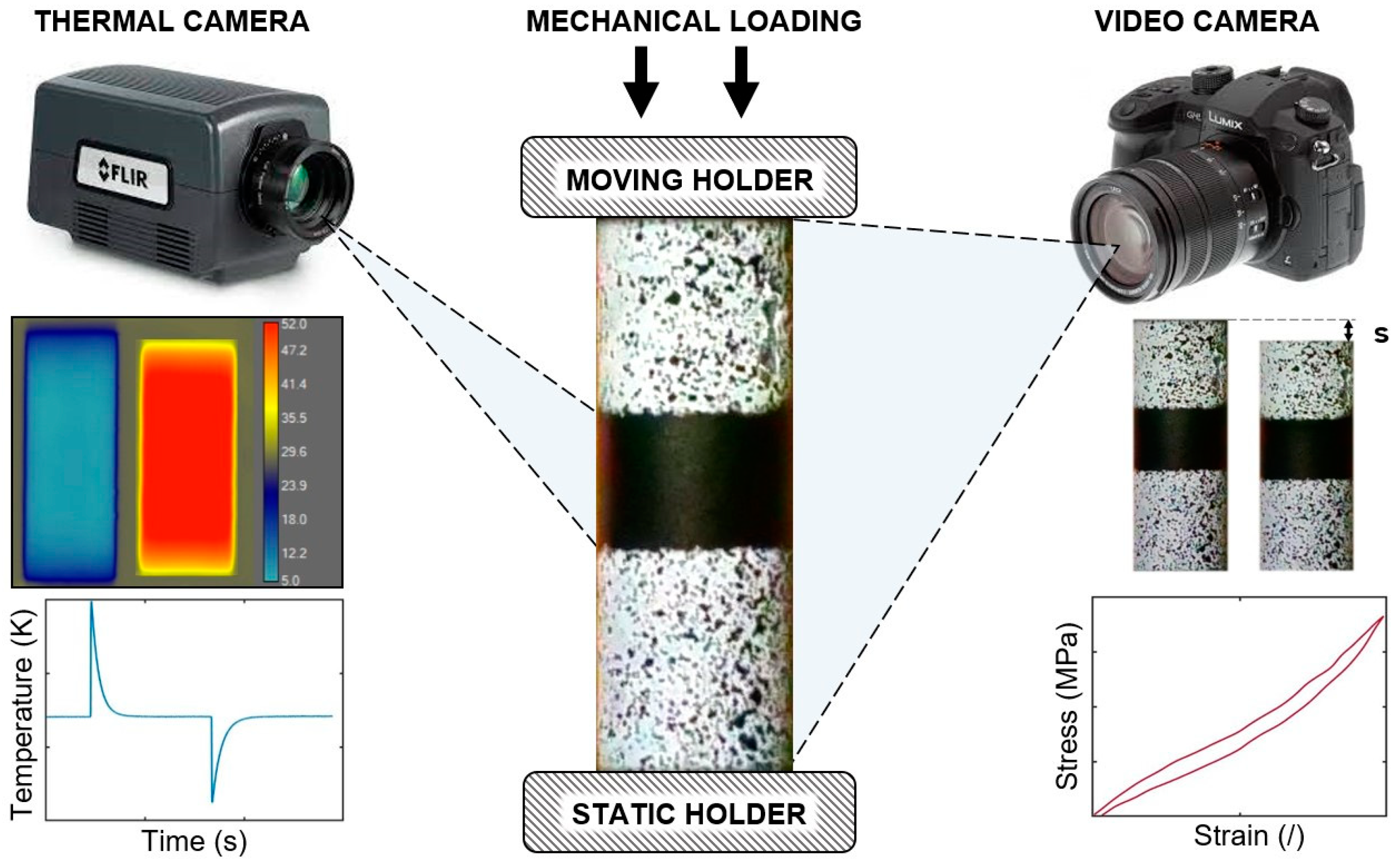
2.1. Experimental Determination of Superelastic and Elastocaloric Properties

In this study, a medical-grade NiTi tube with 55.96 wt% Ni and A_f = −7.3 °C from Memry Corporation, with an outer diameter of 2.5 ± 0.01 mm and an inner diameter of 1.5 ± 0.025 mm, was used. The tube was cut and polished to a length of 29 ± 0.01 mm and inserted into a specially designed holder [66] that provides uniaxial compressive loading. The holder contained two ER collets that held the tube, prevented its movement in the holder (outside the gauge length), and assured uniaxial loading. The gauge length of the tube between the ER collets was 8 mm. Characterization of the superelastic behavior was performed on the Zwick/Roell Z050 Universal Testing Machine (UTM), equipped with a 5 kN load cell (maximum measurement uncertainty of ±0.4% of full scale), and a Zwick/Roell thermostatic chamber. Since the UTM measures the displacement of the crosshead, the measurements included a complex response of the entire system between the crossheads (i.e., tube, holder, clamps). Therefore, the use of an extensometer or a strain gauge was required to accurately measure the strain of the tube. Due to the short gauge length of the specimen (8 mm) and poor accessibility for a mechanical extensometer due to the design of the holder and the size limitations of the thermostatic chamber, a video extensometer was used. The video extensometer was developed in-house and comprised carefully positioned lighting and a Panasonic DC-GH5L camera that recorded the movement of the tube during loading and unloading (a photo of the experimental setup can be found in Figure S2 in the Supplementary materials). Details of the strain measurements with the video-extensometer and their uncertainties, which can be up to 0.2% of the measured value, can be found in [66]. The schematic representation of the experimental setup is shown in Figure 1. The gauge length of the tube was divided into three sections (Figure 1). The middle section was painted with a thermographic paint with high emissivity (ϵ = 0.92), which allows for accurate IR temperature measurements. The upper and lower sections of the tube were painted with white base paint, onto which black speckles were randomly sprayed for video extensometer measurements [66]. The force measurements are made using the UTM’s load cell, where the stress is calculated based on the initial cross-section of the tube.

The objective of the experimental characterization was to obtain the material properties required for the phenomenological model, which was used to simulate superelasticity and later eCE at different temperatures and stresses/strains. Since the numerical model of AeCR requires the elastocaloric data at a very dense set of different temperatures and stresses/strains, phenomenological modeling was necessary because experimental characterization would have been impossible at such a dense set of data. However, the first step of the experimental procedure was to stabilize the superelastic response of the tube through the so-called training. The stress limits and the temperature at which the training was performed were selected with the final application in mind, i.e., the temperatures and stresses at which the eCM will operate in an elastocaloric device. Training temperature was selected based on the highest expected operating temperature of the AeCR and was set at 45 °C. As shown in Tušek et al. [67], training at the highest temperature ensures a stable superelastic response at lower temperatures as long as the maximum applied stress and strain of the training are not exceeded. The stress limit during training was set at 1275 MPa, which is near the end of the transformation plateau of the NiTi tube [66]. The training was performed at a strain rate of 1.75 × 10⁻³ s⁻¹ between 6.5 MPa and 1275 MPa for 100 cycles. During the training, a decrease in the transformation stress, hysteresis loop area, and the recoverable strain can be observed, and the residual strain increases (see Figure 2a), until the response stabilizes towards the end of the training, as previously shown in [67,68]. Figure 2a shows the first and last training cycles. Once the tube was fully stabilized, a series of isothermal and adiabatic tests were performed at room temperature (about 24 °C) and 45 °C. Four strain ranges were applied at each temperature.

Isothermal tests were performed at a strain rate of 5.5 × 10⁻⁵ s⁻¹ (corresponding to the isothermal conditions according to [69]) between 6.5 MPa and a selected upper limit, which was 1100 MPa at 24 °C and 1275 MPa at 45 °C. Figure 2b shows the experimentally measured isothermal superelastic response of the tube at both evaluated temperatures, based on which the material properties (Young’s modulus, transformation strain, martensite peak temperature, and Clausius-Clapeyron coefficient) required for the phenomenological modeling were extracted as explained below. The isothermal superelastic responses at all strains evaluated are shown in the Supplementary materials (Figure S3). As explained and discussed later, the phenomenological model is only used to model the loading curves. Therefore, only the material parameters related to the forward transformation (i.e., the loading curve) are extracted from the experiments. The transformation strain was determined by extrapolating the elastic region of the martensite to zero stress, as shown in Figure 2b. The martensite peak temperature (M_p) and Clausius-Clapeyron coefficient (C_Mp) were determined from the phase diagram of forward transformation (Figure 2c). It was constructed based on the critical stresses defined in the middle of the isothermal transformation plateau for each temperature, as shown in Figure 2b. The hysteresis loop area was calculated using Equation (1) and is shown in Figure 2d as a function of strain, where we can see that the hysteresis loop area increases with both temperature and strain (but only until the end of the transformation). An approximation function was fitted to the experimentally determined hysteresis loop areas, based on which the entropy irreversibilities (Equation (4)) were further calculated for a wider range of strains and temperatures.

$$A_{\mathrm{hyst}}={\displaystyle \oint }\sigma d\epsilon$$

(1)

The experimentally determined NiTi properties needed for further phenomenological modeling are listed in

Table 1. Experimentally determined properties of NiTi tube required for further phenomenological modeling.

EA (GPa)	σAM,24 (MPa)	σAM,45 (MPa)	εtrans (/)	CMp (MPa·K−1)	Mp (K)	Ms (K)	Mf (K)
113.3	463	633	0.0225	7.83	239	315	163

.

After the isothermal tests, the adiabatic tests were performed to evaluate the adiabatic temperature changes, which were then compared to the modeled adiabatic temperature changes (Figure 3b). A thermal imaging camera FLIR A6750sc with a 50 mm focal length lens and an absolute accuracy of ±2% of the temperature reading was used to measure the adiabatic temperature changes. The adiabatic tests were performed at a strain rate of 4.2 × 10⁻² s⁻¹ (corresponding to adiabatic conditions according to [69]) between 6.5 MPa and selected upper limits, which were the same as for the isothermal tests (i.e., 1100 MPa at 24 °C and 1275 MPa at 45 °C). A holding time of 60 s was applied after each adiabatic loading and unloading to allow the temperature of the tube to adjust to the ambient temperature. In this way, we ensured that the temperature conditions for loading and unloading were the same. To assess the repeatability of the measurements, three adiabatic cycles were performed at each applied strain and each temperature and based on this the standard deviations were calculated and included in Figure 3b as error bars. Since the video extensometer and the UTM were not synchronized, the actual strain of the tube could not be controlled (held constant) during the hold time but was instead controlled by the crosshead displacement. As a result, the actual strain of the tube could change to some extent during the holding time (due to the heating or cooling of the tube by heat transfer to the environment). Thus, since the strain of the tube during unloading was not the same as during loading, the measured negative adiabatic temperature changes were not evaluated and considered in the modeling. However, as explained later in the text, the negative adiabatic temperature changes included in the AeCR model were determined by subtracting the temperature irreversibilities due to hysteresis losses from the positive adiabatic temperature changes.

2.2. Phenomenological Modeling

The phenomenological model developed by Tušek et al. [47] was used to model the superelastic behavior. The model describes strain as a function of applied stress and temperature and uses the experimentally determined material properties described in Section 2.1 as input data to predict the full superelastic behavior. Since the phenomenological model presented in [47] can only account for a complete transformation, a different approach is taken in this work to model partial phase transformations as well. Here, the superelastic behavior is calculated only for loading, and the elastocaloric properties are subsequently corrected with the experimentally determined irreversibilities (based on the hysteresis loop area—see Figure 2d) to account for hysteresis behavior. A similar approach was used to model hysteresis losses in magnetocaloric cooling [70]. The superelastic stress-strain response during loading (forward transformation) was modeled with the following equation:

$$\epsilon \left(\sigma ,T\right)=\frac{{\epsilon }_{\mathrm{tran}}}{2}tanh\left(\frac{2.9444}{C_{\mathrm{Mp}} (M_{\mathrm{s}}-M_f)}·\left(\sigma -{\sigma }_{\mathrm{AM}}\left(T\right)\right)\right)+\frac{\sigma }{E_{\mathrm{A}}}+\frac{{\epsilon }_{\mathrm{tran}}}{2}$$

(2)

Figure 3a compares the modeled and experimentally determined superelastic behavior of the NiTi tube during loading where relatively good agreement between both can be seen. Based on the modeled superelastic behavior, the isothermal entropy changes ($\Delta {\mathrm{s}}_{iso}$) during loading were calculated using the Maxwell relation:

$$\Delta s_{\mathrm{iso}}=\frac{1}{\rho }{{\displaystyle \int }}_{{\epsilon }_1}^{{\epsilon }_2}{\left(\frac{\partial \sigma }{\partial T}\right)}_{\mathsf{\epsilon }}dT$$

(3)

Entropy irreversibilities (see Figure 3d) were calculated as a function of strain and temperature based on the hysteresis loop area (Equation (1)) and shown in Figure 2d:

$$\Delta s_{\mathrm{irr}}=\frac{1}{\rho T}{\displaystyle \oint }\sigma d\epsilon =\frac{1}{mT}{A}_{\mathrm{hyst}}$$

(4)

Irreversibilities are included in the numerical model of AeCR as entropy generation during the loading and unloading of the eCM (see Section 3 for details). However, in the next step of the computational process, the total entropy $\left(s_{\mathrm{tot}}^{\prime }=s_{\mathrm{tot}}-s_{\mathrm{tot}}\left(T_1\right)\right)$ was calculated as a function of temperature and strain. It was calculated based on the total entropy at zero applied strain (first term in Equation (5)), where c denotes the baseline specific heat at the reference temperature T₁ (well below the transformation temperatures where transformation can be neglected) and was assumed to be 430 J·kg⁻¹·K⁻¹ [69]. A complete total entropy diagram (Figure 3c) is obtained by adding the values of the isothermal entropy changes (second term in Equation (5)) and subtracting half of the entropy irreversibilities:

$$s_{\mathrm{tot}}^{\prime }\left(\epsilon ,T\right)={\left({{\displaystyle \int }}_{T_1}^{T_2}\frac{c\left(T_1\right)}{T}dT\right)}_{\epsilon =0}+\Delta s_{\mathrm{iso}}\left(\epsilon ,T\right)-\frac{\Delta s_{\mathrm{irr}}\left(\epsilon ,T\right)}{2}$$

(5)

It is assumed that half of the irreversibilities occur during loading and the other half during unloading [61,70]. Based on the obtained T-s′_tot diagram, the specific heat (c) and adiabatic temperature changes ($\Delta T_{\mathrm{ad}}$) can be calculated as follows (both as a function of strain and temperature):

$$c\left(\epsilon ,T\right)=\left(\frac{\partial s_{\mathrm{tot}}^{\prime }\left(\epsilon ,T\right)}{\partial T}\right)T$$

(6)

$$\Delta T_{\mathrm{ad}}\left(\epsilon ,T\right)=T_2\left(s_{\mathrm{tot},\mathsf{\epsilon }}^{\prime },\epsilon \right)-T_1\left(s_{\mathrm{tot},\mathsf{\epsilon }=0}^{\prime },\epsilon =0\right)$$

(7)

When comparing the modeled and experimentally determined adiabatic temperature changes (Figure 3b), the results agree very well. Here it should be noted that the temperature irreversibilities were added to the modeled adiabatic temperature changes for the sake of this comparison. Certain discrepancies between the modeled and experimentally determined adiabatic temperature changes are observed only for the largest applied strains at room temperature. This could be related to the suppression of phase transformation at higher temperatures (during training), which means that the superelastic response is not fully stabilized at lower (room) temperature. This phenomenon needs to be investigated in more detail in the future.

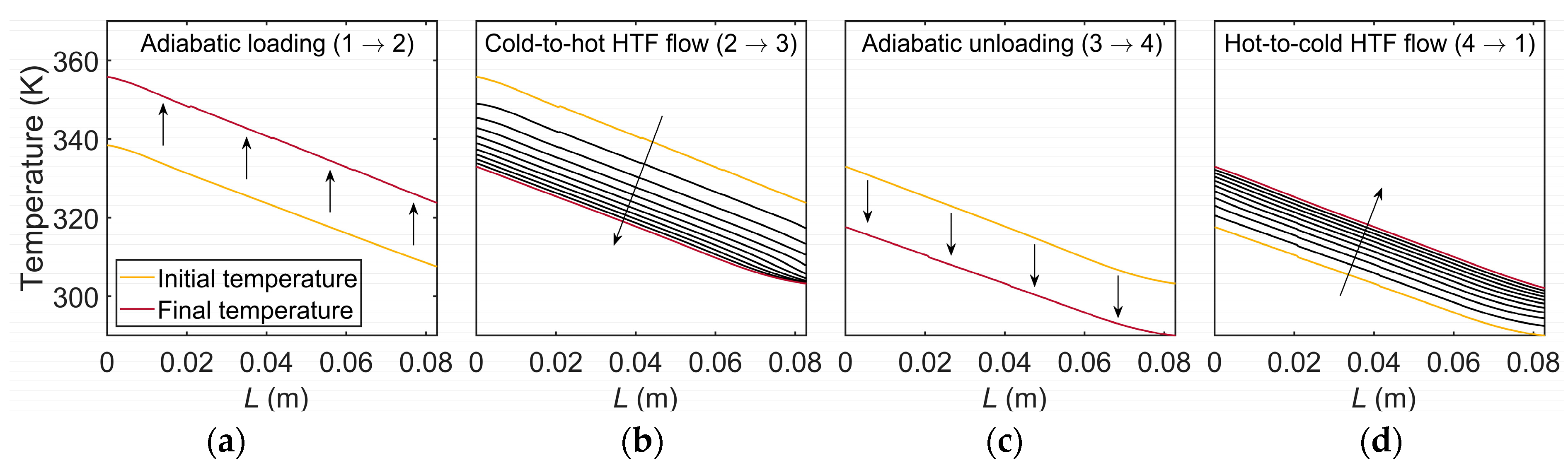
2.3. Numerical Modeling of the AeCR

A transient 1D numerical model originally developed in [65] for a passive shell-and-tube-like regenerator was extended to simulate and optimize the shell-and-tube-like AeCR. The following assumptions were made:

• the HTF flow is incompressible, with no flow maldistributions,
• the HTF properties are defined according to the mean temperature,
• the stress throughout the AeCR is constant,
• the strain within the segment of the AeCR is constant,
• the mechanical loading and unloading are adiabatic,
• a step on and off function of the fluid flow period is assumed,
• the strain is kept constant during the HTF flow period,
• it is assumed that the energy released during unloading is fully recovered.

The governing differential equations of the AeCR model are derived based on the law of energy conservation, taking into account the above assumptions and other assumptions normally used in modeling caloric regenerators [65,71]. The model couples the time-dependent differential equations of three different domains, namely, the heat transfer fluid (HTF) (Equation (8)), the eCM (Equation (9)), and the regenerator housing (Equation (10)), and describes their thermal state and the thermal interaction between the domains. The differential equation of the housing also includes the thermal mass of the supporting elements (baffles, see Figure 4) and takes into account the heat exchange with the environment (heat losses/gains). Considering the geometry specification of the shell-and-tube-like regenerator (Figure 4), Equations (8) and (9) include a term describing the heat transfer through the baffles in the longitudinal direction (Equation (11)). This allows the use of a 1D numerical model where the numerical grid runs along the HTF path, as shown in Figure 4, but still accounts for the heat transfer through the baffles. Adiabatic boundary conditions ($dT/dx=0$) were applied at both ends of the eCM and housing domains, and a temperature boundary condition ($T\left(x=0\right)=T_{\mathrm{in}}$) was set at the inlet of the AeCR in the HTF domain (see [65] for details on the mathematical model and boundary conditions).

$$\frac{\partial T_{\mathrm{f}}}{\partial t}+v\frac{\partial T_{\mathrm{f}}}{\partial x}=\frac{k_{\mathrm{f}}}{{\rho }_{\mathrm{f}}{c}_{\mathrm{f}}}\frac{{\partial }^2{T}_{\mathrm{f}}}{\partial x^2}+h_{\mathrm{ef}}\frac{A_{\mathrm{s}}}{c_{\mathrm{f}}{\dot{m}}_{\mathrm{f}}\tau }\left(T_{\mathrm{s}}-T_{\mathrm{f}}\right)+h_{\mathrm{ef}}\frac{A_{\mathrm{H}}}{c_{\mathrm{f}}{\dot{m}}_{\mathrm{f}}\tau }\left(T_{\mathrm{H}}-T_{\mathrm{f}}\right)+\left|F\frac{2v^3}{d_{\mathrm{h}}{c}_{\mathrm{f}}}\right|-Q_{\mathrm{baf},\mathrm{f}}$$

(8)

$$\frac{\partial T_{\mathrm{s}}}{\partial t}=\frac{k_{\mathrm{s}}}{{\rho }_{\mathrm{s}}{c}_{\mathrm{s}}}\frac{{\partial }^2{T}_{\mathrm{s}}}{\partial x^2}+h_{\mathrm{ef}}\frac{A_{\mathrm{s}}}{c_{\mathrm{s}}{m}_{\mathrm{s}}}\left(T_{\mathrm{f}}-T_{\mathrm{s}}\right)-Q_{\mathrm{baf},\mathrm{s}}$$

(9)

$$\frac{\partial T_{\mathrm{H}}}{\partial t}=\frac{k_{\mathrm{H}}}{{\rho }_{\mathrm{H}}{c}_{\mathrm{H}}}\frac{{\partial }^2{T}_{\mathrm{H}}}{\partial x^2}+h_{\mathrm{ef}}\frac{A_{\mathrm{H}}}{{\rho }_{\mathrm{H}}{c}_{\mathrm{H}}{V}_{\mathrm{H}}}\left(T_{\mathrm{f}}-T_{\mathrm{H}}\right)+\frac{1}{{\rho }_{\mathrm{H}}{c}_{\mathrm{H}}{R}_{\mathrm{a}}{V}_{\mathrm{H}}}\left(T_{\mathrm{a}}-T_{\mathrm{H}}\right)$$

(10)

The heat transfer through the baffles is calculated using the following equation (see Figure 4c):

$$Q_{\mathrm{baf}}=\frac{1}{{\left(\rho cRV\right)}_{\mathrm{baf}}}\left[T\left(x_{\mathrm{i}},y_{\mathrm{j}}\right)-T\left(x_{\mathrm{i}+1},y_{\mathrm{j}+2}\right)\right]$$

(11)

Here, ρ, c, R and V are the density, specific heat, thermal resistance, and volume of the wetted parts of the baffles (made of steel), respectively (see

Table A1. Input parameters to the numerical model.

Material properties
		eCM	HTF		housing
V	(m3)	$2.18·{10}^{-6}$	$2.26·{10}^{-6}$		0.000119
c	(J·kg−1·K−1)	Equation (6)	$f\left(T,p\right)$		726
ρ	(kg·m−3)	6450	$f\left(T,p\right)$		5523
k	(W·m−1·K−1)	8.6/18	$f\left(T,p\right)$		10.9
μ	(Pa·s)	/	$f\left(T,p\right)$		/
Geometrical properties
D	(m)	0.003
d	(m)	0.0025
S	(m)	0.0003
H	(m)	0.008
δsup	(m)	0.004
nt	(/)	18
ns	(/)	4
Aht,L	(m2)	$\pi ·D_{\mathrm{L}}·H·n_{\mathrm{t}}·n_{\mathrm{s}}·\left(1-\epsilon \right)$      for heat transfer from eCM to HTF
		$0.00443·\left(1-\epsilon \right)$                  for heat transfer from HTF to housing
Aht,UL	(m2)	$\pi ·D_{\mathrm{UL}}·H·n_{\mathrm{t}}·n_{\mathrm{s}}$               for heat transfer from eCM to HTF
		0.00443                                 for heat transfer from HTF to housing
Aht,a	(m2)	0.0187
Aht,sup	(m2)	0.00012
dh	(m)	$4\left(\left(S^2\sqrt{3}/4\right)-\left(\pi D^2/8\right)\right)/\left(\pi D/2\right)$				[72]
L	(m)	0.082
Thermohydraulic properties
Re	(/)	$v·d_{\mathrm{h}}·\rho /\mu$
Nu	(/)	$0.051·R{e}^{0.88}·P{r}^{0.36}$				[65]
F	(/)	$3993·R{e}^{-1.4}$				[65]
Ta	(°C)	25 ± 1.5
hout	(W·m−2·K−1)	90
hin	(W·m−2·K−1)	$Nu·k/d_{\mathrm{h}}$
heff	(W·m−2·K−1)	$h_{\mathrm{in}}/\left(1+Bi·\chi \left(Fo\right)/4\right)$ $\mathsf{\chi }\left(Fo\right)=Fo·exp\left[\begin{array}{c}0.246196-0.84878·\ln \left(Fo\right)-\\ 0.05639·{\left(\ln \left(Fo\right)\right)}^2\end{array}\right]$				[83] [84]
Ra	(m2·K·W−1)	$\left({\delta }_{\mathrm{h}}/k_{\mathrm{h}}+1/h_{\mathrm{out}}\right)·A_{\mathrm{ht},\mathrm{a}}$
Rbaf,f	(m2·K·W−1)	$\left({\delta }_{\sup }/k_{\mathrm{Steel}}+2/h_{\mathrm{in}}\right)·A_{\mathrm{ht},\mathrm{baf}}$
Rbaf,s	(m2·K·W−1)	$\left({\delta }_{\sup }/k_{\mathrm{NiTi}}\right)·A_{\mathrm{ht},\mathrm{baf},\mathrm{NiTi}}$

in Appendix A for more details).

In this work, the AeCR numerical model considers four periods of the elastocaloric cooling cycle (e.g., the thermodynamic Brayton cycle). Namely, the adiabatic loading of the eCM, the cold-to-hot HTF flow at constant (high) strain, the adiabatic unloading of the eCM, and the hot-to-cold HTF flow at constant (zero) strain—see the flowchart of the numerical model in Figure S4 in the Supplementary material. The eCE is not directly included in the governing equations, but is applied to the model by considering the appropriate adiabatic temperature changes of the eCM as a function of temperature and strain (see Figure 3b) during loading and unloading. This is related to the assumption of instantaneous mechanical loading/unloading and the associated adiabatic conditions and is only valid if the loading/unloading time is very short so that the adiabatic loading conditions are satisfied. Since the local temperature and local strain of the eCM change during the operation of the AeCR (note that the strain within each segment is assumed to be constant), the adiabatic temperature changes are determined for each node and time step of the cycle as follows: (1) Starting from a global strain (applied to the AeCR as a constant operating condition) and the average temperature of the eCM before loading and unloading, the corresponding stress is determined from the stress-strain curves (Figure 3a). (2) The local strain of each AeCR segment can be determined as a function of the local eCM temperature (in each segment) and the stress along the AeCR (from the stress-strain responses at different temperatures—Figure 3a). Note that the stress is assumed to be constant along the AeCR even though the local temperature and local strain vary. (3) When knowing the strain and temperature of each segment before loading and unloading, the corresponding (non-hysteretic) adiabatic temperature changes can be calculated from the T-s diagram (Figure 3c) using Equation (7). Similarly, the entropy irreversibilities and the specific heat of the eCM can be determined for each strain and temperature (see Equations (4) and (6)). By knowing the (non-hysteretic) adiabatic temperature changes and the entropy irreversibilities the realistic adiabatic temperature changes (including the hysteresis irreversibilities) can be determined for both loading and unloading. As mentioned before, it is assumed that half of the irreversibility occurs during loading and the other half during unloading [61,70] and, therefore, half of the entropy irreversibility is added to the cycle during loading and the other half during unloading.

To approach the real experimental conditions of the AeCR, the geometrical and material properties used as input parameters for the model were taken from our experimentally tested AeCR [35] and are listed in Table A1 in Appendix A. The material properties of housing and NiTi are assumed to be constant, except for the specific heat (c_s) of NiTi, which is calculated using Equation (6). We assumed that the density (ρ) of NiTi is the same for the martensite and austenite phases, although the thermal conductivity (k) of the two phases is different, as shown in Table A1 in Appendix A. The HTF properties included in the model (c, k, ρ, ν) are calculated according to the average temperature of the HTF before each cycle. The heat transfer area of the eCM (A_s) included in the model is only the one in contact with the water, ignoring the portion of the tubes in the baffles since they do not directly contribute to the heat transfer. On the other hand, the mass (m_s) and volume (V_s) of the eCM taken into account in the model also include half of the mass of the tubes in the baffles because, based on our preliminary analysis, we estimate that only about half of the eCM in the baffles transforms (as it is constrained by the baffles) and thus only half of the tubes contributes to active cooling/heating (by heat conduction through the tubes). The AeCR length (fluid flow path) is defined by the active length, i.e., only the length that the HTF passes through the tube bundle (excluding the turns between segments). Since the housing and the baffles are complex in design (see [35] for details), the effective material properties of the housing (ρ_H, c_H, k_H) and its volume (V_H) were calculated based on the volume fraction of each material in the housing assembly (see Table A1 in Appendix A). Heat losses to the surroundings are accounted for in Equation (10) by defining the thermal resistance of the housing (R_a) through each element, as shown in Table A1 in Appendix A.

During loading and unloading, the geometric properties of the AeCR change. The channel height decreases and the tube diameter slightly increases during loading. The latter was studied on a single tube under an applied strain of 3.2% using the Panasonic DC-GH5L camera (see Figure S5 in the Supplementary materials). The increase in diameter at the maximum applied strain was about 2.6% and it was assumed that the increase in diameter has a linear relation with the applied strain. Therefore, the parameters affected by the changes in AeCR geometry (e.g., $A_{\mathrm{s}}, d_{\mathrm{h}}$), are calculated separately for loaded and unloaded AeCR. The hydraulic diameter ($d_{\mathrm{h}}$) is calculated based on the equation normally used for shell-and-tube heat exchangers [72] and is given in Table A1 in Appendix A. The correlations Nu(Re) and F(Re) needed to calculate the convective heat transfer coefficient (h_ef) and the friction factor (F) were taken from [65] where the shell-and-tube-like regenerators were tested for their thermohydraulic properties at operating conditions relevant for such applications (Re < 2000). It should be noted that the governing equations include the effective heat transfer coefficient (h_ef), which takes into account the finite thermal conductivity of the eCM (see Table A1 in Appendix A).

To meet the experimental conditions, the dead volume of 100 mm³ on each side of the AeCR is included in the model. The dead volume is defined as the HTF volume that exits the AeCR but returns to the AeCR in the following fluid flow period instead of flowing toward the heat exchangers, as shown in Figure 4a [73]. In addition, the heat losses/gains of the HTF to/from the environment in the fluid connections between the AeCR and the hot/cold heat exchangers are considered as a heat load on each side of the AeCR (based on the measured values). The latter is applied in the numerical model only for comparison with the experimental results (Section 3.1) and is determined based on the temperature difference between the HTF inlet and outlet temperatures on the cold and hot sides of the AeCR. Heat loads of the fluid connections are omitted from the subsequent analysis of the effects of operating conditions, hysteresis, and heat transfer area on the performance of the AeCR (Section 3.2).

The governing differential equations were discretized using the implicit finite difference approximation. The system of equations was written in matrix notation and was solved using MATLAB software. The influence of the discretization parameters and the convergence criteria are shown in the Supplementary material (Figure S6). The performance of the AeCR is calculated after steady-state conditions are reached (i.e., when the outlet temperatures of the AeCR are periodically stable and do not change by more than 0.0002 K in two consecutive cycles). The temperature span is defined as the difference between the mean outlet temperatures at the hot ($T_{\mathrm{h},\mathrm{o}}$) and cold ($T_{\mathrm{c},\mathrm{o}}$) sides of the regenerator.

$$T_{\mathrm{span}}=\overline{T_{\mathrm{h},\mathrm{o}}}-\overline{T_{\mathrm{c},\mathrm{o}}}$$

(12)

The cooling and heating powers are defined as:

$${\dot{Q}}_{\mathrm{c}}={\dot{m}}_{\mathrm{f}}{c}_{\mathrm{f}}\left(\overline{T_{\mathrm{c},\mathrm{i}}}-\overline{T_{\mathrm{c},\mathrm{o}}}\right)$$

(13)

$${\dot{Q}}_{\mathrm{h}}={\dot{m}}_{\mathrm{f}}{c}_{\mathrm{f}}\left(\overline{T_{\mathrm{h},\mathrm{o}}}-\overline{T_{\mathrm{h},\mathrm{i}}}\right)$$

(14)

Here, ${\dot{Q}}_{\mathrm{c}}$ and ${\dot{Q}}_{\mathrm{h}}$ are the absolute cooling and heating powers, and $T_{\mathrm{c},\mathrm{i}}$, $T_{\mathrm{c},\mathrm{o}}$, $T_{\mathrm{h},\mathrm{o}}$ and $T_{\mathrm{h},\mathrm{i}}$ are the mean inlet and outlet temperatures on the cold and hot sides, respectively. In addition, the efficiency of the AeCR is evaluated by the coefficient of performance (COP), which is defined as the ratio between the cooling/heating power and the input power.

$$CO{P}_{\mathrm{c}\left(\mathrm{h}\right)}=\frac{{\dot{Q}}_{\mathrm{c}\left(\mathrm{h}\right)}}{{\dot{W}}_{\mathrm{mech}}+{\dot{W}}_{\mathrm{pump}}}$$

(15)

Input power includes the mechanical power (${\dot{W}}_{\mathrm{mech}}$) required to load the regenerator and the power required to pump the fluid through the system (${\dot{W}}_{\mathrm{pump}}$). The mechanical input power assumes perfect work recovery during unloading [35] and corresponds to the enclosed area in the stress-strain diagram $\left({\displaystyle \oint }\sigma d\epsilon \right)$ and is calculated as follows:

$${\dot{W}}_{\mathrm{mech}}=f{m}_{\mathrm{s}}{\displaystyle \oint }T ds$$

(16)

Here, $f$ is the operating frequency and $m_{\mathrm{s}}$ is the active mass of eCM in the AeCR. The model was tested for thermodynamic consistency by comparing the required mechanical input power calculated based on the T-s diagram (Equation (16)) and input work calculated from the difference between heating and cooling powers (Equation (17)) when the thermal mass of the housing, heat losses to the surroundings and the frictional losses are excluded.

$${\dot{W}}_{\mathrm{mech},\mathrm{Q}}={\dot{Q}}_{\mathrm{h}}-{\dot{Q}}_{\mathrm{c}}$$

(17)

The power required to pump the fluid (Equation (18)) is calculated based on the pressure drop through the AeCR.

$${\dot{W}}_{\mathrm{pump}}=\frac{{\dot{m}}_{\mathrm{f}}\overline{\Delta p}}{{\rho }_{\mathrm{f}}}$$

(18)

The pressure drop is calculated using Equation (19), which contains the friction factor (F) as a function of the Reynolds number (Re) [65]—see Table A1 in Appendix A for details.

$$\overline{\Delta p}=F\left(Re\right)L{\rho }_{\mathrm{f}}{v}^2/2d_{\mathrm{h}}$$

(19)

In addition, the numerical model was validated against the elastocaloric properties measured on a single tube (at the zero temperature span of the AeCR)—see Supplementary material (Figure S7). Figure S7 shows the contributions of the different effects on the AeCR performance (e.g., hysteresis losses, viscous losses, heat losses to the surroundings, heat capacity of housing, and baffles) in terms of heating power, input power, and COP.

3. Results and Discussion

Before showing the numerically simulated cooling and heating properties of the AeCR, we demonstrate the basic operation of the model. Figure 5a shows the time evolution of the temperature span from the initial state until reaching the steady-state in heat-pumping mode. Figure 5b shows the effect of temperature on local strain during mechanical loading of the AeCR in the steady-state conditions, where the part of the NiTi tube with the highest temperature experiences the lowest strain and thus the smallest adiabatic temperature changes at the specified mechanical load. This so-called eCE degradation due to elevated temperature has already been shown and discussed in [53]. Figure 5c,d show the corresponding elastocaloric cycle in the T-s diagram for the first and steady-state cycles, respectively. In the first cycle, the entire eCM has the same temperature and thus performs the same thermodynamic cycle (Figure 5c). In a steady state, a temperature profile is established and, therefore, each part of the eCM performs its own thermodynamic cycle at a different temperature (Figure 5d). The inset in Figure 5d shows how entropy irreversibility due to hysteresis losses affects the loading of the material (1–2) in the T-s diagram. It can be seen that due to the hysteresis irreversibilities, the adiabatic temperature change during loading is larger than that for the ideal transformation (1–2ⁱ) with $\Delta s_{\mathrm{irr}}=0$. A similar effect occurs during unloading, except that the hysteresis irreversibilities reduce the negative adiabatic temperature changes compared to the ideal transformation. Figure 6 shows the temperature distribution during all four operating steps (a–d) along the HTF path of the eCM in the AeCR after a steady state has been reached.

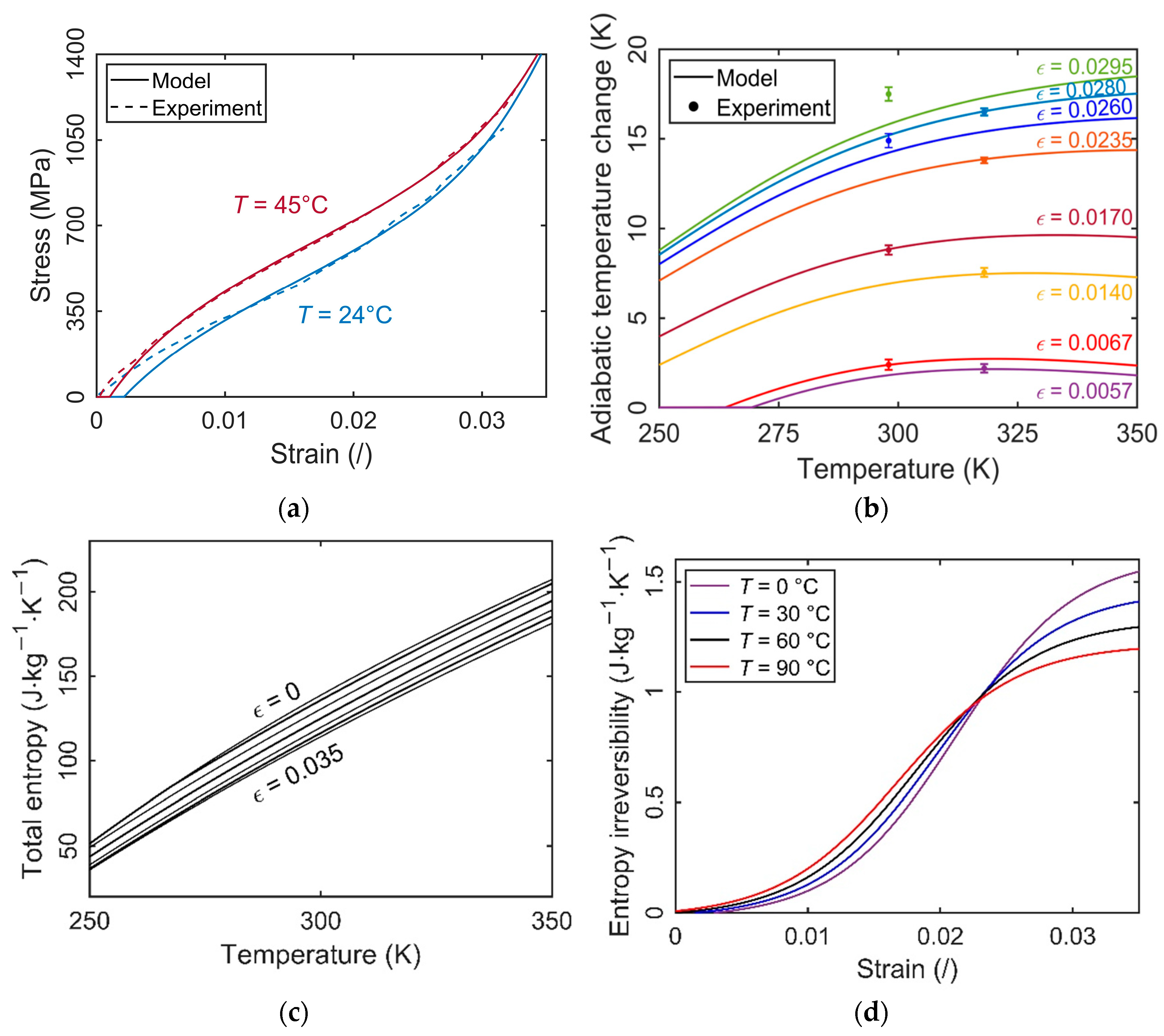
3.1. Model Verification against the Experimental Results

In this section, we present a comparison between the experimentally measured [35] and numerically calculated cooling and heating performance of the shell-and-tube-like AeCR. Figure 7 shows a comparison between the measured [35] and calculated maximum temperature spans established along the AeCR for the heat-pumping and cooling modes at a stress level of 775 MPa (results for 825 MPa are included in the Supplementary materials—see Figures S8–S10). The measurement uncertainty of the temperature span was estimated at ±0.28% [35]. Operating conditions varied in terms of frequency (0.48 Hz, 0.9 Hz, and 2 Hz) and displaced fluid volume ratio (0.18–0.91). The displaced fluid volume ratio is defined as the ratio of the HTF volume displaced through the AeCR in a single fluid flow period to the total volume of fluid in the AeCR as defined by Equation (20).

$$V^{*}=\frac{V_{\mathrm{pump}}}{V_{0,\mathrm{reg}}}=\frac{{\dot{m}}_{\mathrm{f}}{P}_{\mathrm{f}}}{{\rho }_{\mathrm{f}}{V}_{\mathrm{reg}}\epsilon }$$

(20)

The maximum temperature span is reached when the AeCR operates without thermal load, which means that the cooling and heating powers are zero. However, even when there is no external thermal load applied, there were certain heat losses and gains on both sides of the AeCR during the experiments, which were essentially the cooling/heating power from the AeCR’s perspective. These were taken from the experiments (based on the difference between the inlet and outlet temperatures on both sides of the AeCR) [35] and included in the simulations to more accurately describe the operating conditions (for comparison with the experiments only). In the case of the heat-pumping mode, the inlet temperature of the fluid on the cold side was set to 20 °C, and in the case of the cooling mode, the inlet temperature of the fluid on the hot side was set to 30 °C. From Figure 7, it can be seen that the numerical model correctly predicted the increase in the temperature span with increased frequency and stress, and generally also the effect of the displaced fluid volume ratio, although some degree of overestimation of the numerical results is evident. In general, larger deviations were found when the AeCR operated at a smaller displaced volume ratio and higher frequency. This could be related to some malfunctions of the check valves used in the experiments [35], which reduced the performance of the AeCR, especially at small values of the displaced fluid volume ratio and high frequency. For check valves to function properly, a certain pressure difference must be established between the two sides of the check valve, which directly affects the opening and closing times. The pressure difference is smaller for a smaller displaced volume ratio, which can result in HTF leakage before the check valve closes. On the other hand, a higher frequency results in more dynamic operation of the check valves, which means that especially in a combination with a relatively low pressure difference (at a small displaced fluid volume ratio), the effects of improperly opened or closed check valves are more pronounced.

In the second series of simulations, the experimentally measured heating and cooling powers were included in the numerical model. The measurement uncertainty of the cooling/heating power was estimated at ±0.57% [35]. Based on this, the model calculated the corresponding temperature span and the COP (see Equation (15)). Figure 8 shows a comparison between the measured and numerically calculated temperature span—cooling/heating power characteristics. The operating frequency was kept constant at 2 Hz as the effects of three different displaced volume ratios were evaluated. In general, Figure 8 shows relatively good agreement between the numerical and experimental results, but some overestimation can be seen particularly at smaller displaced volume ratios (as already discussed above).

The experimentally measured and numerically calculated regenerator efficiencies were also compared in terms of COP (see Figure 9). The measurement uncertainty of the COP values was estimated at ±3.12% [35]. At a stress level of 775 MPa, the numerical model slightly underestimated the experimentally determined COP. The main reason for the underestimated COP of the numerical model was most likely the overestimated input mechanical work. It should be noted that the mechanical work in the simulations was calculated based on the stress-strain characteristics of the trained single NiTi tube (see Section 2.1). However, as shown in [69], the hysteresis loop area of the NiTi tube was not fully stabilized after 100 training cycles and continued to decrease over up to 500,000 loading cycles, although the adiabatic temperature changes stabilized much earlier. Since the AeCR underwent more than 100,000 cycles before the characterization of the cooling and heat-pumping performance shown here, it was expected that its hysteresis loop area was somewhat smaller than the hysteresis loop area of the single tube used for numerical modeling.

Nevertheless, as shown both experimentally [35] and numerically, the cooling performance of the AeCR was less efficient than that of the heat-pumping, for which there may be several reasons: the eCE itself was not fully reversible due to hysteresis losses in the NiTi resulting in larger adiabatic temperature changes during loading than during unloading; fluid friction and friction between the tube and the baffles were converted to heat; and the geometry when the AeCR was mechanically loaded allowed better heat transfer due to the smaller hydraulic diameter (larger tube diameter).

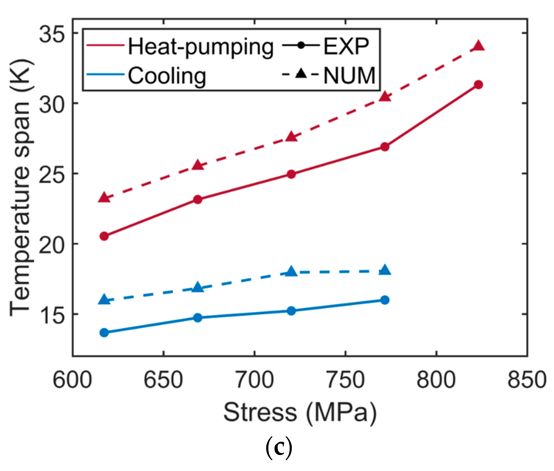
3.2. Impact of the Operating Conditions and Hysteresis Losses

In this section, the influence of operating conditions (applied strain, frequency, and displaced fluid volume ratio) and hysteresis losses on the performance of the shell-and-tube-like AeCR was numerically evaluated. It should be noted that the heat losses and gains on both sides of the AeCR, which were included in the model as cooling/heating power for the purpose of the comparison with the experiments in Section 3.1, were neglected in this set of simulations because it was assumed that they could be minimized by appropriate insulation. Figure 10 shows the effect of applied strain at different operating conditions (operating frequency and displaced fluid volume ratio) on established temperature spans at no thermal load conditions. As expected from the results in Section 3.1, the temperature span increased with increasing strain and frequency, and the increased displaced volume ratio decreased the temperature span. As shown in Figure 10, the temperature span increased almost linearly with strain between about 0.3% and about 3%, corresponding to the transformation plateau (see Figure 2b and Figure 3a) where most of the transformation occurred. At strains above 3%, the temperature span remained almost constant because at these strains the transformation was complete and the eCE remained constant. As predicted by the model, at the maximum applied strain a temperature span of more than 50 K could be reached in the heat-pumping mode and around 45 K in cooling mode at the frequency of 2 Hz and a displaced fluid volume ratio of 0.2.

In the next set of simulations, the cooling/heating powers and the COP values were evaluated at different temperature spans. It should be noted that in this case the temperature span was defined as the temperature difference between both inlet temperatures and not the outlet temperatures, as was the case with calculating the maximum temperature span at no thermal load conditions (see Figure 10 and Equation (14)). In addition, the applied strain was not varied in these simulations and was set to the maximum strain reached during the experiments (2.7%) [35]. Figure 11 shows the cooling/heating power—temperature span and COP—temperature span characteristics of the AeCR at different operating conditions (three different frequencies and three different displaced fluid volume ratios). In general, heating/cooling power and COP increase with decreasing temperature span, as also demonstrated experimentally [35] in Figure 8 and Figure 9. As expected, the maximum heating/cooling power and COP were reached at a zero temperature span. There was a linear trend of both the cooling/heating power—temperature span and COP—temperature span characteristics, as normally observed for single-layered caloric regenerators [71]. One can see from Figure 11a,c that a higher frequency (up to 2 Hz) and displaced fluid volume ratio (up to 1) resulted in a steeper slope of the cooling/heating power-temperature span characteristics. Application of a high frequency (f = 2 Hz) resulted in both a higher temperature span and higher cooling/heating power compared to lower frequencies, and a large displaced fluid volume ratio (V* = 1) resulted in higher cooling/heating power, but a smaller temperature span compared to lower values of displaced fluid volume ratios. The trends were somewhat different regarding the COP values (see Figure 11b,d), where it could be seen that the COP was less affected by the operating frequency, but its dependence on the displaced fluid volume ratio was significant. Similar to the case of cooling/heating power, a high displaced fluid volume ratio resulted in high COP (up to around 3 in the cooling mode and up to around 4 in the heat-pumping mode), but a smaller temperature span. Nevertheless, it should be noted that as the temperature span increased, smaller displaced volume ratios became better, both in terms of heating/cooling powers and COP. Therefore, the amount of heat transfer fluid pumped through the regenerator during the flow period (i.e., the displaced fluid volume ratio) should be adjusted to optimize the performance of the regenerator at a given temperature span.

Based on the results shown in Figure 10 and Figure 11, a threshold temperature span of 15 °C was chosen for further analysis of cooling/heating power and COP. It should be noted that also in this case the temperature span of 15 °C was defined as the temperature difference between both inlet temperatures. Therefore, the inlet fluid temperatures on the cold and hot sides were, in the case of cooling mode, set to 15 °C and 30 °C, and in the case of heat-pumping mode to 20 °C and 35 °C. Figure 12 shows the effects of displaced volume ratio and frequency, on the cooling/heating powers and COP. It can be seen from Figure 12a,c that the heating and cooling power increase with frequency, reaching a peak value of 51 W for the heat-pumping (corresponding to a specific heating power of 3740 W·kg⁻¹) and 12 W for the cooling (corresponding to a specific heating power of 876 W·kg⁻¹), both at the frequency of 4 Hz (i.e., the maximum frequency analyzed). The optimal displaced volume ratio in the heat-pumping mode was around 0.6 and increased slightly with frequency; in the cooling mode it was around 0.5 and increased with frequency up to 2.5 Hz and then started to decrease when the frequency increased further. On the other hand, the COP in the heat-pumping mode increased with frequency, as did the optimal displaced volume ratio (see Figure 12b), and the COP in the cooling mode increased with frequency up to 3.5 Hz and started to decrease at a frequency above 4 Hz (see Figure 12d). A similar trend was expected also for the heat-pumping mode, only at higher frequencies (due to the larger adiabatic temperature changes during loading compared to unloading). The maximum COP values were 1.65 and 0.43 for heat-pumping and cooling, respectively.

Finally, as shown in Figure S7 in the Supplementary material and in the literature [74,75], the hysteresis losses had a significant impact on the COP values and thus the impact of the hysteresis losses on the AeCR performance was studied in more detail. Figure 13 shows the effect of reduced hysteresis losses on the performance of the AeCR at different frequencies at the applied strain of 2.7%, temperature span of 15 °C (based on inlet fluid temperatures), and displaced fluid volume ratio of 0.6. One could see that by reducing the hysteresis, heating power decreased and cooling power increased, since smaller hysteresis results in smaller positive adiabatic temperature changes and larger negative adiabatic temperature changes. The importance of reducing hysteresis was much more pronounced in the case of COP, where significant (up to four times) improvements can be achieved if the material’s hysteresis had been absent, especially in the case of high frequency. Reduced hysteresis is therefore required for achieving higher COP, which could be potentially reached with the development of new materials and improved manufacturing processes in the future [76,77,78,79,80]. Alternatively, the COP can be improved also by applying a more efficient thermodynamic cycle [81,82].

4. Conclusions

A new numerical model for the simulation and optimization of a shell-and-tube-like AeCR was developed. It is based on the governing equations of three different domains of the AeCR, namely the elastocaloric material, heat transfer fluid, and housing. Special attention was paid to the correct evaluation and implementation of the eCE into the AeCR numerical model. For that purpose, an experimental characterization of the eCE of the NiTi tube was performed. Obtained experimental data served as an input to the phenomenological model, which was used to generate a complete set of the elastocaloric data required for AeCR modeling. The hysteresis losses were added to the numerical model separately as entropy irreversibilities during the loading and unloading of the AeCR, obtained from the experimentally determined hysteresis loop areas.

The numerical model was verified against the experimental results from [35], where relatively good agreement between the numerical and experimental results was found in terms of the maximum temperature span, cooling/heating power, and COP for both the heat-pumping and cooling modes. The model correctly predicted the trends of dependency although some overestimations could be observed. The verified model was further used to simulate the shell-and-tube AeCR operation and to evaluate the impact of the applied strain, frequency, displaced fluid volume ratio and reducing the hysteresis losses on its performance. It was found that the performance of the AeCR generally increases with frequency (up to 4 Hz) and applied strain (up to around 3%). The optimal value of the displaced fluid volume ratio strongly depends on the temperature span. High cooling/heating powers (linked to small or zero temperature spans) are reached at small displaced fluid volume ratios (e.g., V* = 0.2), and high temperature spans (linked to small or zero cooling/heating power) are reached at higher displaced fluid volume ration (e.g., V* = 1). As calculated by the model, the maximum temperature spans (at zero cooling/heating power) of more than 50 K in the heat-pumping mode and around 45 K in the cooling mode could be reached, both at the operating frequency of 2 Hz, displaced fluid volume ratio of 0.2, and applied strain above 3%. In the cooling mode, the maximum cooling power of 41 W (corresponding to the specific cooling power of 2990 W·kg⁻¹ of eCM) and COP of around 3 were obtained at zero temperature span, operating frequency of 2 Hz, displaced fluid volume ratio of 1, and applied strain of 2.7%, and in the heat-pumping mode, the maximum heating power of 54 W (corresponding to the specific cooling power of 3940 W·kg⁻¹ of eCM) and the maximum COP of around 4 were obtained under the same operating conditions. At a temperature span of 15 K, cooling power of 8.5 W (620 W·kg⁻¹ of eCM) and COP of 0.45 were obtained in the cooling mode, and in the heat-pumping mode, the heating power of 27 W (1970 W·kg⁻¹ of eCM) and COP of 1.4 were obtained at a frequency of 4 Hz and applied strain of 2.7%. We demonstrated that the main source of irreversibility that results in rather low COP values is the hysteresis of the eCM. The COP could be increased up to four times if the material with no hysteresis but the same eCE could be applied. Therefore, it is crucial to study an eCM with smaller hysteresis, which can be achieved by using a different eCM (e.g., Cu-based SMAs or some Heusler alloys) and modifying the microstructure of the NiTi alloys (e.g., grain size).

In our future work, the developed and verified numerical model will be used to further optimize the AeCR. In particular, we will investigate the effects of the geometry of the eCM, different eCMs with different elastocaloric properties, different HTFs, etc., on the AeCR performance. In addition, we will model and study layered AeCR with different eCMs along its length, where each eCM will have optimized transformation temperatures according to different working temperatures along the AeCR. Different thermodynamic cycles of the AeCR will also be studied and optimized. Finally, the impact of the efficiency of the work recovery during the unloading on the COP of the AeCR will be studied as well.

References

1. Ozone Secretariat. Handbook for the Montreal Protocol on Substances That Deplete the Ozone Layer, 14th ed.; Ozone Secretariat: Nairobi, Kenya, 2020. [Google Scholar]
2. Kauffeld, M. Current long-term alternative refrigerants and their applications. In Proceedings of the 31st Informatory Note on Refrigeration Technologies, International Institute of Refrigeration, Paris, France, 1 April 2016. [Google Scholar]
3. McLinden, M.O.; Brown, J.S.; Brignoli, R.; Kazakov, A.F.; Domanski, P.A. Limited options for low-global-warming-potential refrigerants. Nat. Commun. 2017, 8, 14476. [Google Scholar] [CrossRef] [PubMed] [Green Version]
4. IEA. Average Efficiency of New Air Conditioners 2000–2020 and in the Net Zero Scenario; IEA: Paris, France; Available online: https://www.iea.org/data-and-statistics/charts/average-efficiency-of-new-air-conditioners-2000-2020-and-in-the-net-zero-scenario (accessed on 12 September 2022).
5. Kitanovski, A. Energy Applications of Magnetocaloric Materials. Adv. Energy Mater. 2020, 10, 1903741. [Google Scholar] [CrossRef]
6. Ismail, M.; Yebiyo, M.; Chaer, I.A. Review of Recent Advances in Emerging Alternative Heating and Cooling Technologies. Energies 2021, 14, 502. [Google Scholar] [CrossRef]
7. Goetzler, W.; Zogg, R.; Young, J.; Johnson, C. Energy Savings Potential and RD & D Opportunities for Non-Vapor-Compression HVAC Technologies; United States Department of Energy: Washington, DC, USA, 2014; p. 3673. [CrossRef]
8. OECD/IEA. The Future of Cooling Opportunities for Energy-Efficient Air Conditioning Together Secure Sustainable. 2018. Available online: www.iea.org/t&c/ (accessed on 12 September 2022).
9. Bruederlin, F.; Bumke, L.; Chluba, C.; Ossmer, H.; Quandt, E.; Kohl, M. Elastocaloric Cooling on the Miniature Scale: A Review on Materials and Device Engineering. Energy Technol. 2018, 6, 1588–1604. [Google Scholar] [CrossRef]
10. Kalizan, J.; Tušek, J. Caloric Micro-Cooling: Numerical modelling and parametric investigation. Energy Convers. Manag. 2020, 225, 113421. [Google Scholar] [CrossRef]
11. Babapoor, A.; Aziz, M.; Karimi, G. Thermal management of a Li-on battery using carbon fiber-PCM composites. Appl. Therm. Eng. 2015, 62, 281–290. [Google Scholar] [CrossRef]
12. Bo, Z.; Li, Z.; Yang, H.; Li, C.; Wu, S.; Xu, C.; Xiong, G.; Mariotti, D.; Yan, J.; Cen, K.; et al. Combinatorial atomistic-to-AI prediction and experimental validation of heating effects in 350 F supercapacitor modules. Int. J. Heat Mass Transf. 2021, 171, 121075. [Google Scholar] [CrossRef]
13. Kabirifar, P.; Žerovnik, A.; Ahčin, Ž.; Porenta, L.; Brojan, M.; Tušek, J. Elastocaloric Cooling: State-of-the-art and Future Challenges in Designing Regenerative Elastocaloric Devices. J. Mech. Eng. 2019, 65, 615–630. [Google Scholar] [CrossRef] [Green Version]
14. Rodriguez, C.; Brown, L.C. The thermal effect due to stress-induced martensite formation in Β-CuAlNi single crystals. Metall. Mater. Trans. A 1980, 11, 147–150. [Google Scholar] [CrossRef]
15. Hou, H.; Qian, S.; Takeuchi, I. Materials, physics and systems for multicaloric cooling. Nat. Rev. Mater. 2022, 7, 633–652. [Google Scholar] [CrossRef]
16. Qian, S. Thermodynamics of elastocasloric cooling and heat pump cycles. Appl. Therm. Eng. 2023, 219, 119540. [Google Scholar] [CrossRef]
17. Frenzel, J.; Wieczorek, A.; Opahle, I.; Maaß, B.; Drautz, R.; Eggeler, G. On the effect of alloy composition on martensite start temperatures and latent heats in Ni–Ti-based shape memory alloys. Acta Mater. 2015, 90, 213–231. [Google Scholar] [CrossRef]
18. Wieczorek, A.; Frenzel, J.; Schmidt, M.; Maass, B.; Seelecke, S.; Schütze, A.; Eggeler, G. Optimizing Ni–Ti-based shape memory alloys for ferroic cooling. Funct. Mater. Lett. 2017, 10, 1740001. [Google Scholar] [CrossRef]
19. Chluba, C.; Ge, W.; de Miranda, R.L.; Strobel, J.; Kienle, L.; Quandt, E.; Wuttig, M. Ultralow-fatigue shape memory alloy films. Science 2015, 348, 1004–1007. [Google Scholar] [CrossRef] [PubMed]
20. Chluba, C.; Ossmer, H.; Zamponi, C.; Kohl, M.; Quandt, E. Ultra-Low Fatigue Quaternary TiNi-Based Films for Elastocaloric Cooling. Shape Mem. Superelasticity 2016, 2, 95–103. [Google Scholar] [CrossRef] [Green Version]
21. Mañosa, L.; Jarque-Farnos, S.; Vives, E.; Planes, A. Large temperature span and giant refrigerant capacity in elastocaloric Cu-Zn-Al shape memory alloys. Appl. Phys. Lett. 2013, 103, 211904. [Google Scholar] [CrossRef]
22. Qian, S.; Geng, Y.; Wang, Y.; Pillsbury, T.E.; Hada, Y.; Yamaguchi, Y.; Fujimoto, K.; Hwang, Y.; Radermacher, R.; Cui, J.; et al. Elastocaloric effect in CuAlZn and CuAlMn shape memory alloys under compression. Philos. Trans. R. Soc. A Math. Phys. Eng. Sci. 2016, 374, 20150309. [Google Scholar] [CrossRef] [Green Version]
23. Xiao, F.; Bucsek, A.; Jin, X.; Porta, M.; Planes, A. Giant elastic response and ultra-stable elastocaloric effect in tweed textured Fe-Pd single crystals. Acta Mater. 2022, 223, 117486. [Google Scholar] [CrossRef]
24. Liu, J.; Zhao, D.; Li, Y. Exploring Magnetic Elastocaloric Materials for Solid-State Cooling. Shape Mem. Superelasticity 2017, 3, 192–198. [Google Scholar] [CrossRef]
25. Tong, W.; Liang, L.; Xu, J.; Wang, H.J.; Tian, J.; Peng, L.M. Achieving enhanced mechanical, pseudoelastic and elastocaloric properties in Ni-Mn-Ga alloys via Dy micro-alloying and isothermal mechanical cyclic training. Scr. Mater. 2022, 209, 114393. [Google Scholar] [CrossRef]
26. Zhang, S.; Yang, Q.; Li, C.; Fu, Y.; Zhang, H.; Ye, Z.; Zhou, X.; Li, Q.; Wang, T.; Wang, S.; et al. Solid-state cooling by elastocaloric polymer with uniform chain-lengths. Nat. Commun. 2022, 13, 9. [Google Scholar] [CrossRef] [PubMed]
27. Bennacer, R.; Liu, B.; Yang, M.; Chen, A. Refrigeration performance and the elastocaloric effect in natural and synthetic rubbers. Appl. Therm. Eng. 2022, 204, 117938. [Google Scholar] [CrossRef]
28. Imran, M.; Zhang, X. Recent developments on the cyclic stability in elastocaloric materials. Mater. Des. 2020, 195, 109030. [Google Scholar] [CrossRef]
29. Chen, J.; Lei, L.; Fang, G. Elastocaloric cooling of shape memory alloys: A review. Mater. Today Commun. 2021, 28, 102706. [Google Scholar] [CrossRef]
30. Imran, M.; Zhang, X. Reduced dimensions elastocaloric materials: A route towards miniaturized refrigeration. Mater. Des. 2021, 206, 109784. [Google Scholar] [CrossRef]
31. Tušek, J.; Engelbrecht, K.; Eriksen, D.; Dall’Olio, S.; Tušek, J.; Pryds, N. A regenerative elastocaloric heat pump. Nat. Energy 2016, 1, 16134. [Google Scholar] [CrossRef]
32. Kirsch, S.M.; Welsch, F.; Michaelis, N.; Schmidt, M.; Wieczorek, A.; Frenzel, J.; Eggeler, G.; Schütze, A.; Seelecke, S. NiTi-Based Elastocaloric Cooling on the Macroscale: From Basic Concepts to Realization. Energy Technol. 2018, 6, 1567–1587. [Google Scholar] [CrossRef]
33. Chen, J.; Zhang, K.; Kan, Q.; Yin, H.; Sun, Q. Ultra-high fatigue life of NiTi cylinders for compression-based elastocaloric cooling. Appl. Phys. Lett. 2019, 115, 93902. [Google Scholar] [CrossRef]
34. Snodgrass, R.; Erickson, D. A multistage elastocaloric refrigerator and heat pump with 28 K temperature span. Sci. Rep. 2019, 9, 18532. [Google Scholar] [CrossRef]
35. Ahčin, Ž.; Dall’Olio, S.; Žerovnik, A.; Baškovič, U.Ž.; Porenta, L.; Kabirifar, P.; Cerar, J.; Zupan, S.; Brojan, M.; Klemenc, J.; et al. High-performance cooling and heat pumping based on fatigue-resistant elastocaloric effect in compression. Joule 2022, 6, 2338–2357. [Google Scholar] [CrossRef]
36. Bachmann, N.; Fitger, A.; Maier, L.M.; Mahlke, A.; Schäfer-Welsen, O.; Koch, T.; Bartholomé, K. Long-term stable compressive elastocaloric cooling system with latent heat transfer. Commun. Phys. 2021, 4, 194. [Google Scholar] [CrossRef]
37. Chen, Y.; Wang, Y.; Sun, W.; Qian, S.; Liu, J. A compact elastocaloric refrigerator. Innovation 2022, 3, 100205. [Google Scholar] [CrossRef] [PubMed]
38. Zhang, J.; Zhu, Y.; Cheng, S.; Yao, S.; Sun, Q. Enhancing cooling performance of NiTi elastocaloric tube refrigerant via internal grooving. Appl. Therm. Eng. 2022, 213, 118657. [Google Scholar] [CrossRef]
39. Emaikwu, N.; Catalini, D.; Muehlbauer, J.; Hwang, Y.; Takeuchi, I.; Radermacher, R. Experimental Investigation of a Staggered-Tube Active Elastocaloric Regenerator. Int. J. Refrig. 2022, in press. [CrossRef]
40. Li, X.; Cheng, S.; Sun, Q. A compact NiTi elastocaloric air cooler with low force bending actuation. Appl. Therm. Eng. 2022, 215, 118942. [Google Scholar] [CrossRef]
41. Barclay, J.A.; Steyer, W.A. Active Magnetic Regenerator. U.S. Patent 4332135A, 1 June 1982. [Google Scholar]
42. Torelló, A.; Lheritier, P.; Usui, T.; Nouchokgwe, Y.; Gérard, M.; Bouton, O.; Hirose, S.; Defay, E. Giant temperature span in electrocaloric regenerator. Science 2020, 370, 125–129. [Google Scholar] [CrossRef] [PubMed]
43. Han, Y.; Lai, C.; Li, J.; Zhang, Z.; Zhang, H.; Hou, S.; Wang, F.; Zhao, J.; Zhang, C.; Miao, H.; et al. Elastocaloric cooler for waste heat recovery from proton exchange membrane fuel cells. Energy 2022, 238, 121789. [Google Scholar] [CrossRef]
44. Al-Hamed, K.H.M.; Dincer, I.; Rosen, M.A. Investigation of elastocaloric cooling option in a solar energy-driven system. Int. J. Refrig. 2020, 120, 340–356. [Google Scholar] [CrossRef]
45. Qian, S.; Ling, J.; Hwang, Y.; Radermacher, R.; Takeuchi, I. Thermodynamics cycle analysis and numerical modeling of thermoelastic cooling systems. Int. J. Refrig. 2015, 56, 65–80. [Google Scholar] [CrossRef]
46. Luo, D.; Feng, Y.; Verma, P. Modeling and analysis of an integrated solid state elastocaloric heat pumping system. Energy 2017, 130, 500–514. [Google Scholar] [CrossRef]
47. Tušek, J.; Engelbrecht, K.; Millán-Solsona, R.; Mañosa, L.; Vives, E.; Mikkelsen, L.P.; Pryds, N. The Elastocaloric Effect: A Way to Cool Efficiently; Supporting Information. Adv. Energy Mater. 2015, 5, 1500361. [Google Scholar] [CrossRef]
48. Qian, S.; Wang, Y.; Xu, S.; Chen, Y.; Yuan, L.; Yu, J. Cascade utilization of low-grade thermal energy by coupled elastocaloric power and cooling cycle. Appl. Energy 2021, 298, 117269. [Google Scholar] [CrossRef]
49. Sebald, G.; Komiya, A.; Jay, J.; Coativy, G.; Lebrun, L. Regenerative cooling using elastocaloric rubber: Analytical model and experiments. J. Appl. Phys. 2020, 127, 94903. [Google Scholar] [CrossRef]
50. Zhu, Y.; Hur, J.; Cheng, S.; Sun, Q.; Li, W.; Yao, S. Modelling of elastocaloric regenerators with enhanced heat transfer structures. Int. J. Heat Mass Transf. 2021, 176, 121372. [Google Scholar] [CrossRef]
51. Tušek, J.; Engelbrecht, K.; Pryds, N. Elastocaloric effect of a Ni-Ti plate to be applied in a regenerator-based cooling device. Sci. Technol. Built Environ. 2016, 22, 489–499. [Google Scholar] [CrossRef]
52. Tan, J.; Wang, Y.; Xu, S.; Liu, H.; Qian, S. Thermodynamic cycle analysis of heat driven elastocaloric cooling system. Energy 2020, 197, 117261. [Google Scholar] [CrossRef]
53. Qian, S.; Wang, Y.; Yuan, L.; Yu, J. A heat driven elastocaloric cooling system. Energy 2019, 182, 881–899. [Google Scholar] [CrossRef]
54. Qian, S.; Yuan, L.; Yu, J.; Yan, G. Numerical modeling of an active elastocaloric regenerator refrigerator with phase transformation kinetics and the matching principle for materials selection. Energy 2017, 141, 744–756. [Google Scholar] [CrossRef]
55. Cirillo, L.; Rosaria Farina, A.; Greco, A.; Masselli, C. The optimization of the energy performances of a single bunch of elastocaloric elements to be employed in an experimental device. Therm. Sci. Eng. Prog. 2022, 27, 101152. [Google Scholar] [CrossRef]
56. Qian, S.; Yuan, L.; Hou, H.; Takeuchi, I. Accurate prediction of work and coefficient of performance of elastocaloric materials with phase transformation kinetics. Sci. Technol. Built Environ. 2018, 24, 673–684. [Google Scholar] [CrossRef]
57. Ulpiani, G.; Saliari, M.; Bruederlin, F.; Kohl, M.; Ranzi, G.; Santamouris, M. On the cooling potential of elastocaloric devices for building ventilation. Sol. Energy 2021, 230, 298–311. [Google Scholar] [CrossRef]
58. Bachmann, N.; Schwarz, D.; Bach, D.; Schäfer-Welsen, O.; Koch, T.; Bartholomé, K. Modeling of an Elastocaloric Cooling System for Determining Efficiency. Energies 2022, 15, 5089. [Google Scholar] [CrossRef]
59. Heintze, O.; Seelecke, S. A coupled thermomechanical model for shape memory alloys-From single crystal to polycrystal. Mater. Sci. Eng. A 2008, 481–482, 389–394. [Google Scholar] [CrossRef]
60. Yuan, L.; Wang, Y.; Yu, J.; Greco, A.; Masselli, C.; Qian, S. Numerical study of a double-effect elastocaloric cooling system powered by low-grade heat. Appl. Therm. Eng. 2023, 218, 119302. [Google Scholar] [CrossRef]
61. Bachmann, N.; Fitger, A.; Unmüßig, S.; Bach, D.; Schäfer-Welsen, O.; Koch, T.; Bartholomé, K. Phenomenological model for first-order elastocaloric materials. Int. J. Refrig. 2022, 136, 245–253. [Google Scholar] [CrossRef]
62. Hess, T.; Vogel, C.; Maier, L.M.; Barcza, A.; Vieyra, H.P.; Schäfer-Welsen, O.; Wöllenstein, J.; Bartholomé, K. Phenomenological model for a first-order magnetocaloric material. Int. J. Refrig. 2020, 109, 128–134. [Google Scholar] [CrossRef]
63. Griffith, L.D.; Alho, B.P.; Czernuszewicz, A.; Ribeiro, P.O.; Slaughter, J.; Pecharsky, V.K. Toward efficient elastocaloric systems: Predicting material thermal properties with high fidelity. Acta Mater. 2021, 217, 117162. [Google Scholar] [CrossRef]
64. de Oliveira, N.A.; von Ranke, P.J. Theoretical aspects of the magnetocaloric effect. Phys. Rep. 2010, 489, 89–159. [Google Scholar] [CrossRef]
65. Ahčin, Ž.; Liang, J.; Engelbrecht, K.; Tušek, J. Thermo-hydraulic evaluation of oscillating-flow shell-and-tube-like regenerators for (elasto)caloric cooling. Appl. Therm. Eng. 2021, 190, 116842. [Google Scholar] [CrossRef]
66. Porenta, L.; Trojer, J.; Brojan, M.; Tušek, J. Experimental investigation of buckling stability of superelastic Ni-Ti tubes under cyclic compressive loading: Towards defining functionally stable tubes for elastocaloric cooling. Int. J. Solids Struct. 2022, 256, 111948. [Google Scholar] [CrossRef]
67. Tušek, J.; Engelbrecht, K.; Mikkelsen, L.P.; Pryds, N. Elastocaloric effect of Ni-Ti wire for application in a cooling device. J. Appl. Phys. 2015, 117, 124901. [Google Scholar] [CrossRef] [Green Version]
68. Miyazaki, S.; Imai, T.; Igo, Y.; Otsuka, K. Effect of cyclic deformation on the pseudoelasticity characteristics of Ti-Ni alloys. Metall. Trans. A 1986, 17, 115–120. [Google Scholar] [CrossRef]
69. Porenta, L.; Kabirifar, P.; Žerovnik, A.; Cebron, M.; Žužek, B.; Dolenec, M.; Brojan, M.; Tušek, J. Thin-walled Ni-Ti tubes under compression: Ideal candidates for efficient and fatigue-resistant elastocaloric cooling. Appl. Mater. Today 2020, 20, 100712. [Google Scholar] [CrossRef]
70. Brey, W.; Nellis, G.; Klein, S. Thermodynamic modeling of magnetic hysteresis in AMRR cycles. Int. J. Refrig. 2014, 47, 85–97. [Google Scholar] [CrossRef] [Green Version]
71. Kitanovski, A.; Tušek, J.; Tomc, U.; Plaznik, U.; Ožbolt, M.; Poredoš, A. Magnetocaloric Energy Conversion—From Theory to Applications; Springer: Berlin, Germany, 2015. [Google Scholar] [CrossRef]
72. Žukauskas, A. Heat Transfer from Tubes in Crossflow. Adv. Heat Transf. 1987, 18, 87–159. [Google Scholar] [CrossRef]
73. Trevizoli, P.V.; Barbosa, J.R. Thermal-hydraulic behavior and influence of carryover losses in oscillating-flow regenerators. Int. J. Therm. Sci. 2017, 113, 89–99. [Google Scholar] [CrossRef]
74. Masche, M.; Ianniciello, L.; Tušek, J.; Engelbrecht, K. Impact of hysteresis on caloric cooling performance. Int. J. Refrig. 2021, 121, 302–312. [Google Scholar] [CrossRef]
75. Hess, T.; Maier, L.M.; Bachmann, N.; Corhan, P.; Schäfer-Welsen, O.; Wöllenstein, J.; Bartholomé, K. Thermal hysteresis and its impact on the efficiency of first-order caloric materials. J. Appl. Phys. 2020, 127, 75103. [Google Scholar] [CrossRef]
76. Lu, B.; Song, M.; Zhou, Z.; Liu, W.; Wang, B.; Lu, S.; Wu, C.; Yang, L.; Liu, J. Reducing mechanical hysteresis via tuning the microstructural orientations in Heusler-type Ni44.8Mn36.9In13.3Co5.0 elastocaloric alloys. J. Alloys Compd. 2019, 785, 1023–1029. [Google Scholar] [CrossRef]
77. Yuan, B.; Zhu, X.; Zhang, X.; Qian, M. Elastocaloric effect with small hysteresis in bamboo-grained Cu–Al–Mn microwires. J. Mater. Sci. 2019, 54, 9613–9621. [Google Scholar] [CrossRef]
78. Ahadi, A.; Kawasaki, T.; Harjo, S.; Ko, W.S.; Sun, Q.; Tsuchiya, K. Reversible elastocaloric effect at ultra-low temperatures in nanocrystalline shape memory alloys. Acta Mater. 2019, 165, 109–117. [Google Scholar] [CrossRef]
79. Zhu, X.; Zhang, X.; Qian, M. Reversible elastocaloric effects with small hysteresis in nanocrystalline Ni-Ti microwires. AIP Adv. 2018, 8, 125002. [Google Scholar] [CrossRef]
80. Lin, H.; Hua, P.; Sun, Q. Effects of grain size and partial amorphization on elastocaloric cooling performance of nanostructured NiTi. Scr. Mater. 2022, 209, 114371. [Google Scholar] [CrossRef]
81. Kabirifar, P.; Trojer, J.; Brojan, M.; Tušek, J. From the elastocaloric effect towards an efficient thermodynamic cycle. J. Phys. Energy 2022, 4, 44009. [Google Scholar] [CrossRef]
82. Schmidt, M.; Kirsch, S.M.; Seelecke, S.; Schütze, A. Elastocaloric cooling: From fundamental thermodynamics to solid state air conditioning. Sci. Technol. Built Environ. 2016, 22, 475–488. [Google Scholar] [CrossRef]
83. Jeffreson, C.P. Prediction of breakthrough curves in packed beds: II. Experimental evidence for axial dispersion and intraparticle effects. AIChE J. 1972, 18, 416–420. [Google Scholar] [CrossRef]
84. Engelbrecht, K.L.; Nellis, G.F.; Klein, S.A. The effect of internal temperature gradients on regenerator matrix performance. J. Heat Transf. 2006, 128, 1060–1069. [Google Scholar] [CrossRef]
Figure 1. Schematic representation of the experimental setup for superelastic and elastocaloric characterization of the tube, showing the tube with the marked regions of interest for the thermal camera and video extensometer measurements.
Energies 15 09253 g001
Figure 2. The first and last training cycles and determination of EA and EM (a); isothermal superelastic stress-strain behavior at 24 °C and 45 °C and determination of transformation strain and critical stress at the middle of the transformation (b); the phase diagram for the forward transformation showing the martensite peak temperature and the corresponding Clausius-Clapeyron coefficient (c); and the isothermal hysteresis loop area as a function of strain for both evaluated temperatures (d).
Energies 15 09253 g002
Figure 3. Comparison of experimentally determined and modeled superelastic behavior at different temperatures (a); comparison of experimentally determined and modeled positive adiabatic temperature changes during loading (b); entropy-temperature diagram (c); Modelled entropy irreversibilities as a function of strain at different temperatures (d).
Energies 15 09253 g003
Figure 4. CAD model of the shell-and-tube AeCR: cross-sectional view (a); longitudinal view with a schematic representation of the 1D discretization of regenerators’ domain (b); and schematic representation of the heat transfer through the baffles in the 1D domain (c).
Energies 15 09253 g004
Figure 5. Time evolution of the temperature span of HTF outlet temperatures (a); presentation of the modeled loading curves at three different temperatures (b); presentation of the modeled active elastocaloric cycle in the T-s diagram with detail of the inclusion of irreversibility in the case of the first cycle (c) and the steady-state cycle (d).
Energies 15 09253 g005
Figure 6. Evolution of the eCM temperature profile along the AeCR during each phase of the thermodynamic cycle.
Energies 15 09253 g006
Figure 7. Comparison between experimentally determined and numerically calculated maximum temperature spans established along the AeCR under different operating conditions for heat-pumping (a) at a stress level of 775 MPa and cooling (b) and under different mechanical loads (c).
Energies 15 09253 g007aEnergies 15 09253 g007b
Figure 8. Comparison between experimentally determined and numerically calculated temperature span—cooling/heating power characteristics for heat-pumping (a) and cooling (b) at a stress level of 775 MPa.
Energies 15 09253 g008
Figure 9. Comparison between experimentally determined and numerically calculated COP—cooling/heating power characteristics for heat-pumping (a) and cooling (b) at the stress level of 775 MPa.
Energies 15 09253 g009
Figure 10. The effect of different applied strains at different operating conditions (operating frequency and displaced fluid volume ratio) on established temperature spans at no thermal load conditions for heat-pumping (a) and cooling (b).
Energies 15 09253 g010
Figure 11. The effect of temperature span on AeCR performance at a fixed strain of 2.7% for heat-pumping (a,b) and cooling (c,d).
Energies 15 09253 g011
Figure 12. The effect of displaced volume ratio and frequency on AeCR performance at a fixed strain of 2.7% and temperature span of 15 K (based on inlet fluid temperatures) for heat-pumping (a,b) and cooling (c,d).
Energies 15 09253 g012
Figure 13. The effect of reduced hysteresis losses on the performance of the AeCR at a fixed strain of 2.7%, temperature span of 15 K and displaced fluid volume ratio of 0.6 for heat-pumping (a,b) and cooling (c,d).
Energies 15 09253 g013