Aerodynamic Configuration Optimization of a Propeller Using Reynolds-Averaged Navier–Stokes and Adjoint Method

Abstract

The discrete adjoint method was used to optimize the aerodynamic configuration in order to increase the efficiency and precision of design. The fully unstable simulation of propeller rotation was avoided using the quasi approach. In the meantime, the gradient-based optimization approach was extended to the rotating coordinate in which the propeller blades were running, thereby increasing the dimension of the shape parameters as multi-coordinates were taken into account. However, the precision of the propeller optimization was improved by expanding the range of variation for design parameters. Using the current design framework, the propeller’s torsion angle, blade chord length, and blade profile were modified independently by an optimization solver, resulting in a notable acceleration.

1. Introduction

The propeller is a critical component of many aerodynamic devices, such as turboprops and industrial ventilation. Although nearly 80% efficiency can be obtained from the design by the Wright brothers [1], the requirements relating to environmental issues, carrying capacity, and voyage lengths have provoked people to develop more efficient propeller with low emissions and high performance. Many works have been done from different points of view, for example, optimizing the shape, upgrading the materials, or inventing new propulsion system. The first approach should be the most efficient and direct way to achieve the requirement of optimization, which, in many cases, is to find the minimum drag under given constraints. The strategies to find the most optimized solution of shape deformation of propeller via an intelligent algorithm, by which the globally optimized solution could be found in theory, have been widely used due to the fast development of computational fluid dynamics (CFD) approach. Avoiding a mass of computation caused by low convergence rate and the high-dimensional optimization problem, the pioneering work conducted by Hicks et al. [2] was the landmark of the two-dimensional profile optimization design. However, most of these algorithms are black-box finite difference methods. Vanderplaats et al. [3], and the common issues, such as step-size limitation and the huge computing cost with the increasing number of design parameters, which is often the case with aerodynamic design application, for these algorithms hinder them from being extended to more complex geometry. Pironneau [4] formulated the elliptic design problem, which is very common in aircraft design, via the control theory, and the cost was decreased dramatically, that is, the gradient information of objective function with respect to the design variables was estimated through a set of adjoint equations. Although the extra overhead of solving the adjoint equations may bring additional time consumption, the benefit that if the gradient of cost function being obtained still is more attractive. A series of works about shape optimization for Euler and Navier–Stokes equations have been performed by [5,6,7,8], and these works injected the optimization theory into the process of design, which, certainly, inspires the researchers to solve the complex problems with this method. Only a single flow solution and a single adjoint solution are needed for calculating the sensitivity derivatives of the objective function with respect to any numbers of design variables, which will provide independence between computing consumption and the dimension of design space.

Considering the aerodynamic optimization of a propeller, the classical vortex theories, all of which can be seen as the development of vortex line theory by Lerbs [9], are the most-used method for the performance evaluation of propeller in a fast manner. The works starting from 1960s, see, for example, the works of Kerwin [10,11,12] about marine propeller numerical simulation and design, and those of [13,14,15] about turbofan of airplanes. In addition, some more recent researches of, e.g., Xiang et al. and Alba et al. [16,17], still optimized the propeller based on the results from vortex-theory-based methods. These methods, however, cannot provide reliable results when some important details about the flow through the propeller are missing, such as the viscous effect. Unlike the stable parts of an airplane, an accurate prediction of the propeller should be an unsteady process due to the rotating blades, this, indeed, will need a very long time to achieve a converged solution and a complex mesh treatment technology for the solver. The Moving Reference Frame (MRF) can be regarded as a compromise between unsteady simulation and the vortex-theory-based methods. The flow around the propeller is treated in a steady-state manner with the local reference frame rotating at the design speed, and the governing equations are solved while the additional accelerating terms are considered. The most obvious advantage of MRF is the effect of Reynolds, and Mach number varying is included, by which the airfoils at different radial locations can be optimized separately. Meanwhile, some crucial parameters, such as the viscous effect and the distribution of chord length must be considered if a higher efficiency is needed [18]. In addition, the three-dimension effect, e.g., crossflow, on the blades of a propeller, with which the vortex-based-theory can not be involved, is another important factor for the propeller design. Based on the adjoint methods, Allen et al. [19] investigated the twist optimization on a hovering rotors with 15 design parameters, see also the works of Dumont et al., Allen et al., Farrokhfal et al., and Dhert et al. [20,21,22,23].

In the present work, the enhancement of aerodynamic performance CFD-based subsonic propeller by the adjoint method is conducted. Compared with the low fidelity models, the RANS solver provided some complex phenomena which will be presented in present paper, and the information that comes from these details can result in a reliable design certainly. The focus of the present work is on demonstrating the potential of CFD-based propeller optimization under the subsonic flow condition. Three geometrical parameters: profiles of the blade, chord length distribution of the blades, and the torsional angle. In total, 116 design variables are considered in present work.

2. Numerical Methodology

2.1. Governing Equations

The compressible Navier–Stokes equations are considered here. The equations are written in conservative form in an inertial reference frame, and this form is suite for both moving or stationary control volume, viz.,

$$\frac{\partial }{\partial t}\underset{D}{\int }\overrightarrow{Q}dD+\underset{\Gamma }{\oint }\left({\mathit{F}}_{\mathit{C}}-{\mathit{F}}_{\mathit{D}}\right)d\Gamma =0$$

(1)

where $\overrightarrow{Q}$ indicates the vector of conservative variables which has the following form:

$$\overrightarrow{Q}={\left(\rho ,\rho u,\rho v,\rho w,\rho E\right)}^T$$

(2)

The computational domain D are bounded by the surface $\Gamma$ with a outward unit normal vector $\overrightarrow{n}={(n_x,n_y,n_z)}^T$ expressed in $R_r$. The convective flux and diffusive flux are expressed as:

$${\mathit{F}}_{\mathit{C}}=\left(\begin{array}{c}\rho (\overrightarrow{V}-{\overrightarrow{V}}_e)·n\\ \rho u(\overrightarrow{V}-{\overrightarrow{V}}_e)·n+p{n}_x\\ \rho v(\overrightarrow{V}-{\overrightarrow{V}}_e)·n+p{n}_y\\ \rho w(\overrightarrow{V}-{\overrightarrow{V}}_e)·n+p{n}_z\\ \rho E(\overrightarrow{V}-{\overrightarrow{V}}_e)·n+pV·n\end{array}\right)$$

(3)

$${\mathit{F}}_{\mathit{D}}=\left(\begin{array}{c}0\\ (\tau +{\tau }_R)·n\\ (\tau +{\tau }_R)·V·n-(\Phi +{\Phi }_T)·n\end{array}\right)$$

(4)

where $\overrightarrow{V}={(u,v,w)}^T$ and ${\overrightarrow{V}}_e={(u_e,v_e,w_e)}^T$ are the velocity vector of flow with respect to $R_a$ and the convective velocity of $R_r$. Both of these two vectors are expressed in $R_r$. The variables $\tau$ and ${\tau }_R$ denote the shear stress tensor and Reynolds stress tensor. In addition, $\Phi$ and ${\Phi }_t$ are the heat flux vector and Reynolds heat flux vector. In the Equation (1), the source term S represents the influence of the Coriolis force. If considering a mass of air itself stirred by a propeller turning around the streamwise direction($\mathit{x}$ axis), the exact formulation of S is:

$$S={(0,0,-\Omega \rho w,\Omega \rho v,0)}^T$$

(5)

The equation of state for a perfect gas is used in the mean flow equations, viz.,

$$p=(\gamma -1)(E-\rho \frac{u^2+v^2+w^3}{2})$$

(6)

2.2. Numerical Method

An in-house solver $Xenium$, which works on unstructured mesh, is used in the present paper. The governing equations shown above are discretized via a finite volume method, and the conservative flow variables are expressed with cell-centered evaluation. ${\mathit{F}}_{\mathit{C}}$ is discretized using flux difference formula developed by Roe [24] and MUSCL approach [25] with Venkatakrishnan limiter [26], however, no limiter is used in present paper. The turbulence model used in present paper is proposed by Spalart and Allmaras [27]. A centered formula is used for the diffusive flux ${\mathit{F}}_{\mathit{D}}$. The gradients of velocity and temperature are evaluated at the center of each cell interface. For turbulent flow, the Boussinesq assumption is used for Reynolds stress tensor. The eddy viscosity is calculated with the Spalart–Allmaras model [27], which is loosely coupled to the mean-flow equations. A backward Euler time-differencing scheme is used to update the solution, and the linear system of equations is approximately solved with a multicolor point-implicit procedure or an implicit-line relaxation scheme at each time step [28].

The DLR-F6 wingbody, which served as one of the standard test models in Drag Prediction Workshop II [29], is used here for demonstration of the code precision. The design cruise Mach number for DLR-F6 is $Ma=0.75$, and the lift coefficient is $C_L=0.5$. Three sets of mesh are denoted as coarse, medium, and fine. It should be noted that the distances of the first node away from the wall, normalized with friction velocity and molecular viscous, are less than 1 of all meshes, which could provide a proper description of viscous sub-layer.

The Case 1 in the workshop, which denoted a transonic cruise condition with a constant lift, was selected here to demonstrate the precision of the code. The simulation was run at a Reynolds number $Re=3\times {10}^6$ based on geometric chord with fully-turbulent flow condition.

Table 1. Aerodynamic characteristics of the DLR-F6 wing body.

Mesh	Total Nodes	Angle of Attack	${\mathit{C}}_{\mathit{L}}$	${\mathit{C}}_{\mathit{D}}$	${\mathit{C}}_{\mathit{Dp}}$	${\mathit{C}}_{\mathit{Df}}$
Coarse	1,119,145	0.055	0.5	0.032030	0.01875351	0.01327652
Medium	3,092,999	0.250	0.5	0.030676	0.01751588	0.01316048
Fine	6,829,375	0.450	0.5	0.030363	0.01733237	0.01303149
Exp	\	0.520	0.5	0.0295	\	\

demonstrates the angle of attack, pressure drag, viscous drag, and total drag. As the grid refinement, the drag coefficient is close to the experimental value. The larger decrease part of $C_D$ comes from the pressure drag, which mainly is determined by spatial distribution of mesh. The predicted coefficient by the present solver, which is shown in Figure 1 is reasonable when take the results from DPW-II with some other solvers [29].

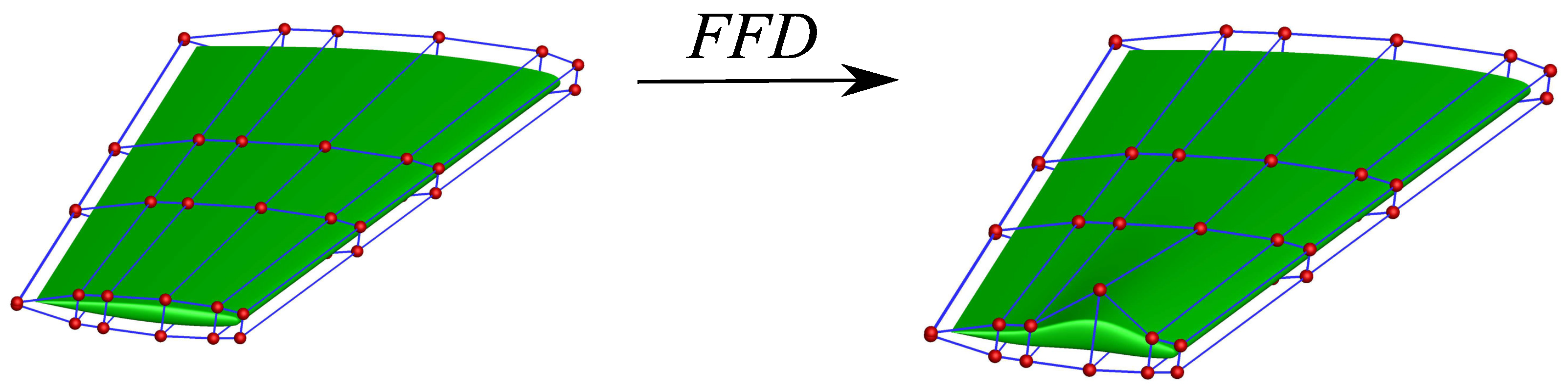
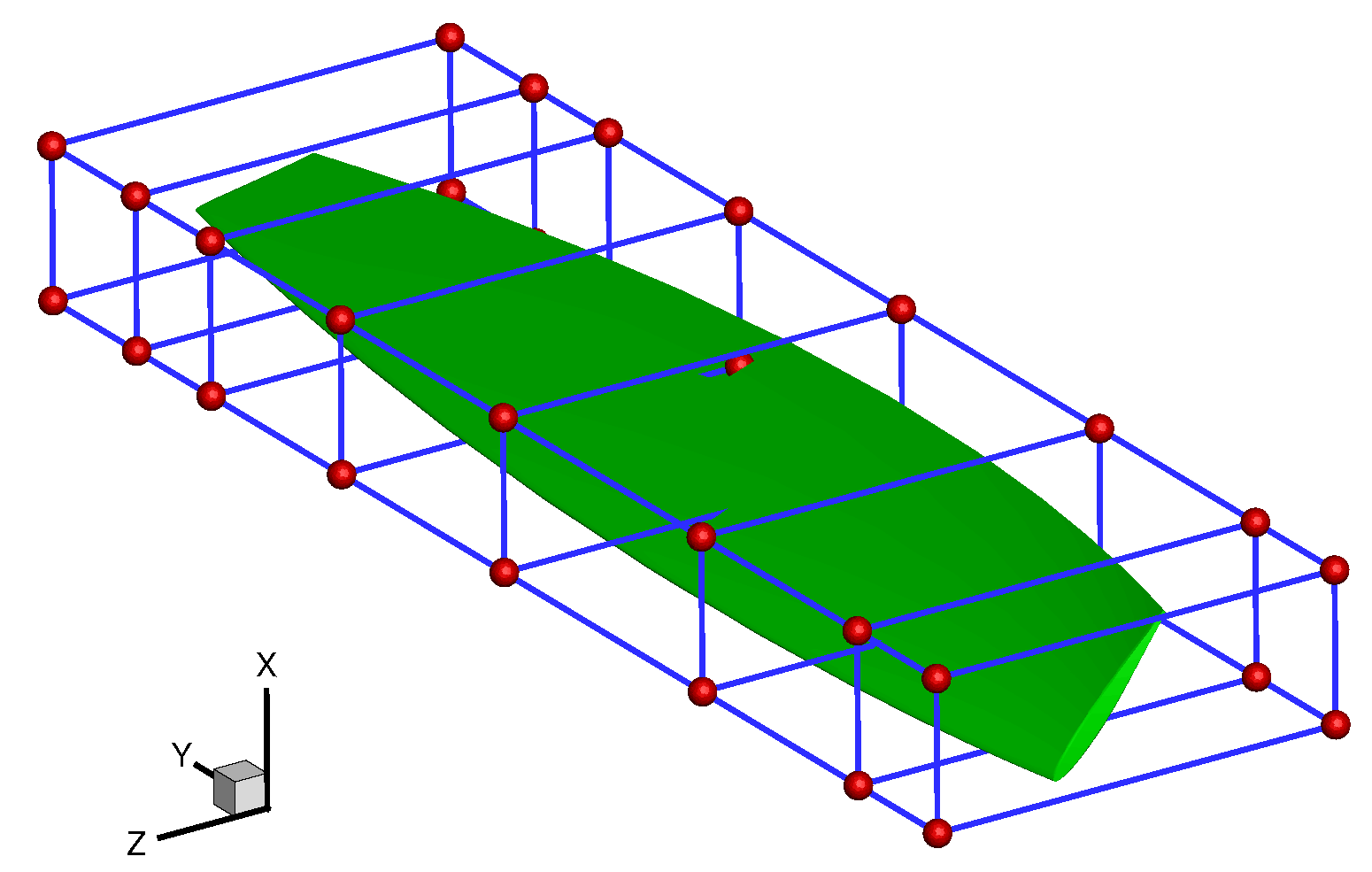
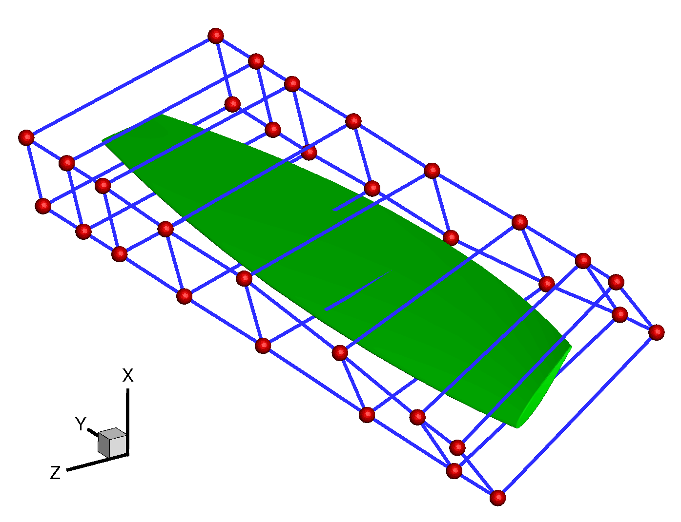
2.3. Shape and Mesh Deformation

The configuration of the propeller is parameterized by different distributions of twist, chord length, and the airfoil of the blades. The free-form deformation (FFD) developed by Samareh [30] was used herein and the geometry is parameterized by the coordinates of the lattice box points, which allows a broad range of deformations with a low number of parameters and a smooth deformation. Namely, the geometry (i.e., the surface mesh of the airfoil, blades, wing, etc.) which is parameterized as a B$\acute{e}$zier solid. The lattice box can be expressed by the following formulation:

$$X(s,t,u)=X_0+\sum _{i,j,k=1}^{l,m,n}{P}_{i,j,k}{B}_i^l\left(s\right)B_j^m\left(t\right)B_k^n\left(u\right)$$

(7)

where s, t, u$\in [0,1]$ are the three components of the local coordinate, respectively. The $X_0$ stands for the original point of the local coordinate. $B^i$ is the Bernstein polynomial of order i. Then, the relation between Cartesian coordinates on the surface mesh and the FFD box was built. The shape of the surface mesh can be changed through varying the control points (design variables) of the box. An example of FFD control point deformation to a wing geometry demonstrates in Figure 2.

The sensitivity of the surface mesh to design variables should be calculated to use the discrete adjoint approach:

$$\frac{d{\mathit{G}}_{\mathit{s}}}{d\overrightarrow{\beta }}=\frac{\partial {\mathit{G}}_{\mathit{s}}}{\partial {\mathit{G}}_{\mathit{FFD}}}\frac{\partial {\mathit{G}}_{\mathit{FFD}}}{\partial \overrightarrow{\beta }}$$

(8)

where the ${\mathit{G}}_{\mathit{s}}$ and ${\mathit{G}}_{\mathit{FFD}}$ denote surface mesh coordinate and displacement vector of the control points on FFD box, $\overrightarrow{\beta }$ the design variables vector. The gradient $\partial {\mathit{G}}_{\mathit{s}}/\partial {\mathit{G}}_{\mathit{FFD}}$ can be obtained by using Equation (7), viz.

$$\frac{\partial X(s,t,u)}{\partial P_{i2,j2,k2}}=\sum _{i,j,k=1}^{l,m,n}\left(B_i^l\left(s\right)B_j^m\left(t\right)B_k^n\left(u\right)\sum _{i,j,k=2}^{l,m,n}\frac{\partial P_{i1,j1,k1}}{\partial }{P}_{i2,j2,k2}\right)$$

(9)

where the $P_{i2,j2,k2}$ is the control point’s Cartesian coordinates referred in the gradient, while the $P_{i1,j1,k1}$ denotes the control point’s Cartesian coordinates according to its subscripts on the FFD box. In this paper, the combined movement of control points will be introduced by $\partial G_{FFD}/\partial x$. Hence, the movement of control point will be considered independently in Equation (9).

The mesh deformation approach in present work was treated as a linear elasticity problem, which has been found to be a very robust method in practice. If the body force is neglected, the linear elasticity equations in differential form are:

$$\Delta ·\overline{\overline{\sigma }}=0$$

(10)

where $\overline{\overline{\sigma }}$ is the stress tensor given by

$$\overline{\overline{\sigma }}=\lambda Tr\left(\overline{\overline{ϵ}}\right)\overline{\overline{I}}+2\mu \overline{\overline{ϵ}}$$

(11)

where $Tr$ is the trace of strain tensor

$$\overline{\overline{ϵ}}=\frac{1}{2}\left(\frac{\partial u_i}{\partial x_j}+\frac{\partial u_j}{\partial x_i}\right)$$

(12)

with $\mathit{u}$=($u_1,u_2,u_3{)}^T$ being the displacement vector. Considering the code used herein is finite-volume-method, and integrating the Equation (10) with Gauss’ Theorem gives:

$${\mathit{R}}_{\mathit{el}}\left(\mathit{u}\right)={\oint }_{\partial V}\lambda \frac{\partial u_i}{\partial x_i}\overline{\overline{I}}·\widehat{\mathit{n}}dS+{\oint }_{\partial V}\mu \left(\frac{\partial u_i}{\partial x_j}+\frac{\partial u_j}{\partial x_i}\right)·\widehat{\mathit{n}}dD=0$$

(13)

After giving an initial assumption of ${\mathit{u}}_{\mathbf{0}}$, the displacement vector $\mathit{u}={\mathit{u}}_{\mathbf{0}}+\Delta \mathit{u}$ is substituted into Equation (13). The following system of linear equations for $\Delta \mathit{u}$ is expressed as:

$$\frac{\partial {\mathit{R}}_{\mathit{el}}}{\partial \mathit{u}}\Delta \mathit{u}=-{\mathit{R}}_{\mathit{el}}\left({\mathit{u}}_{\mathbf{0}}\right)$$

(14)

The Jacobian $\partial {\mathit{R}}_{\mathit{el}}/\partial \mathit{u}$ does not depend on $\mathit{u}$ due to the Equation (13) is linear, hence the equation above can be solved via generalized minimum residual (GMRES) method [31]. The material properties $\lambda$ and $\mu$ can be determined by Young’s modulus E and Poisson’s relation.

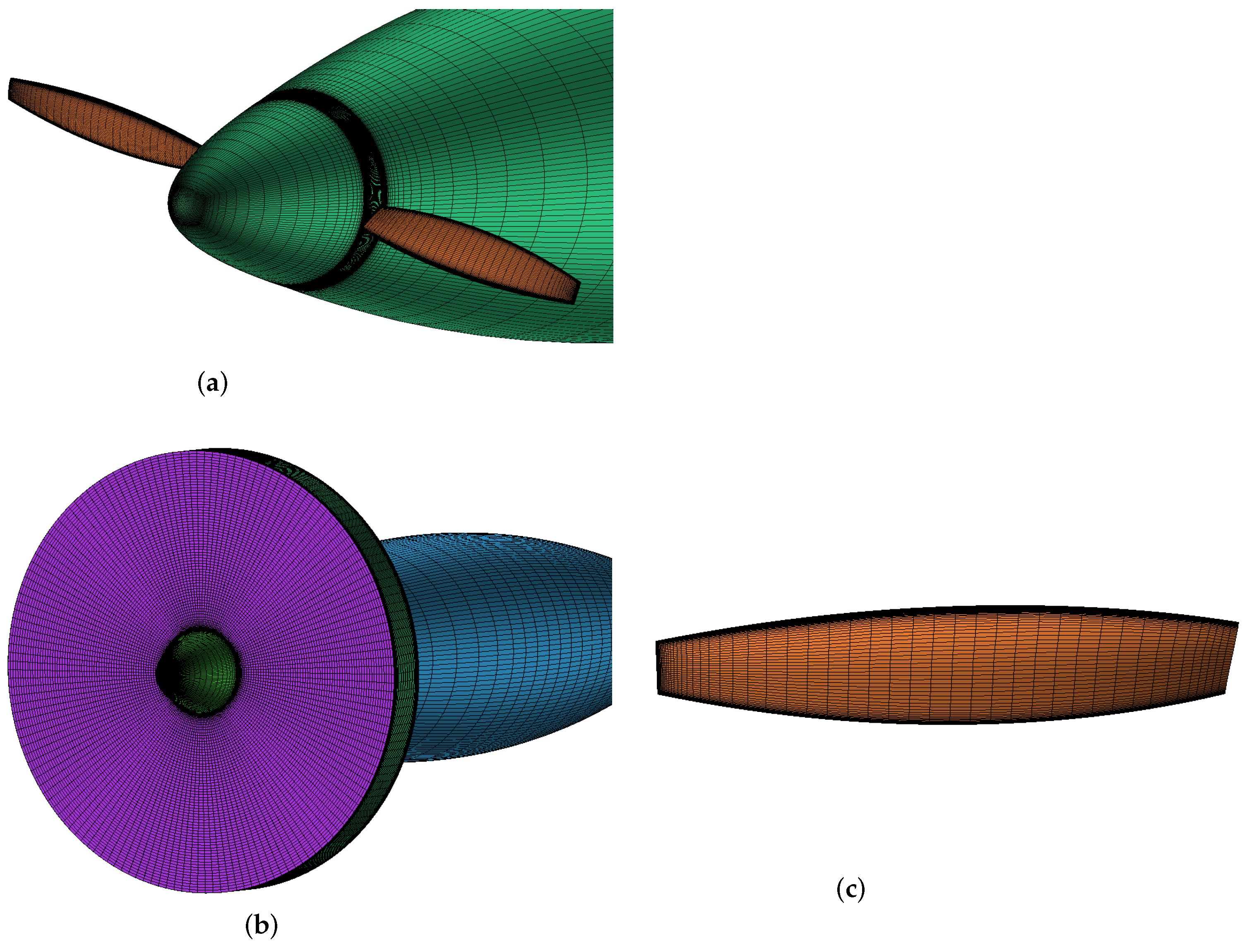
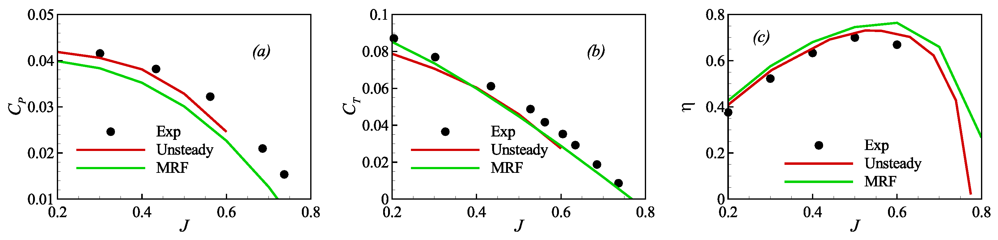
2.4. The MRF Approach

The rotation of the propeller is modeled using the Moving Reference Frame (MRF) method. Namely, the unsteady rotation of the propeller is formulated in a non-inertial reference frame rotating with the body, and the problem becomes steady and then a dramatic reduction in computation cost can be achieved. In present code, the governing equations are solved by adding extra acceleration terms which are induced by rotation. The absolute velocity $\overrightarrow{v}$ and the relative velocity $\overrightarrow{v_r}$ are related according to the following equation:

$$\overrightarrow{v_r}=\overrightarrow{v}-(\overrightarrow{\Omega }\times \overrightarrow{r})$$

(15)

where $\overrightarrow{r}$ is the position vector from the origin point of rotating frame and $\overrightarrow{\Omega }$ is the angular velocity vector. There are two ways to express the governing equation, that is, by absolute velocity formulation or relative velocity formulation. If we wrote the equations by relative velocity formulation:

$$\frac{\partial \rho }{\partial t}+\nabla ·\left(\rho \overrightarrow{v_r}\right)=0$$

(16)

$$\frac{\partial \left(\rho \overrightarrow{v_r}\right)}{\partial t}+\nabla ·\left(\rho \overrightarrow{v_r}\overrightarrow{v_r}+p\overline{\overline{I}}-\overline{\overline{\tau }}\right)=-2\rho (\overrightarrow{\Omega }\times \overrightarrow{v_r})-\rho \overrightarrow{\Omega }\times (\Omega \times \overrightarrow{r})$$

(17)

$$\frac{\partial E_r}{\partial t}+\nabla ·\left[\overrightarrow{v_r}(E_r+p)+k\nabla T-\overline{\overline{\tau }}·\overrightarrow{v_r}\right]=0$$

(18)

The two terms on the right-hand side of the momentum equation are Coriolis force per unit volume and the centrifugal force per unit volume, respectively. $E_r=p/(\gamma -1)+\frac{1}{2}\rho |\overrightarrow{v_r}{|}^2-\frac{1}{2}\rho |\overrightarrow{\Omega }\times \overrightarrow{r}|=E-\rho \overrightarrow{v_r}·(\overrightarrow{\Omega }\times \overrightarrow{r})$ is the total energy per unit volume in the rotating frame.

A low-Reynolds-number propeller with spinner and nacelle tested by Ghoddoussi [32] is used herein to validate the MRF approach. The propeller is right-handed, with a diameter D of 0.3 m, and the corresponding Reynolds number vary from 90,000 to 120,000 in the experiment. The rotational speed is 6000 rpm. The profiles are given in the Ref. [32], and the twist angle along the spanwise can be obtained from a function $\beta =1714.5/r$ with r the radius. The chord length distribution is $c=-0.0033r^2+0.6r-4.5$. The computed mesh used in present work is shown in Figure 3. The no-slip boundary condition is used for propeller surface, and a MRF region is defined to surround the whole propeller. The pressure-field boundary condition is used for the box which locates at 100c and involves all geometries. Roughly 4.3 million mesh cells are used in present computation.

The main performance coefficients of the present propeller are advance ratio $J=0.2\sim 0.8$, defined as:

$$J=\frac{U_{\infty }}{nD}$$

(19)

where $U_{\infty }$ is the freestream velocity. In addition, the efficiency $\eta$, trust coefficient $K_T$, and the torque coefficient $K_Q$ are defined in the following equations:

$$\eta =\frac{J{K}_T}{2\pi K_Q};K_T=\frac{T}{\rho n^2{D}^4};K_Q=\frac{T}{\rho n^2{D}^5}$$

(20)

where T is the thrust, P is power of the propeller, and $\rho$ is density. The experimental data come from the work done by Ghoddoussi [32], and the unsteady simulation results is obtained by ANSYS CFX with a global time-step $\Delta t=5.56\times {10}^{-5}s$. The results cover a length of advance ratio $J=0.2\sim 0.6$. Figure 4 contains comparison of thrust, power and efficiency coefficient of the propeller.

3. Flowfield Adjoint Equations

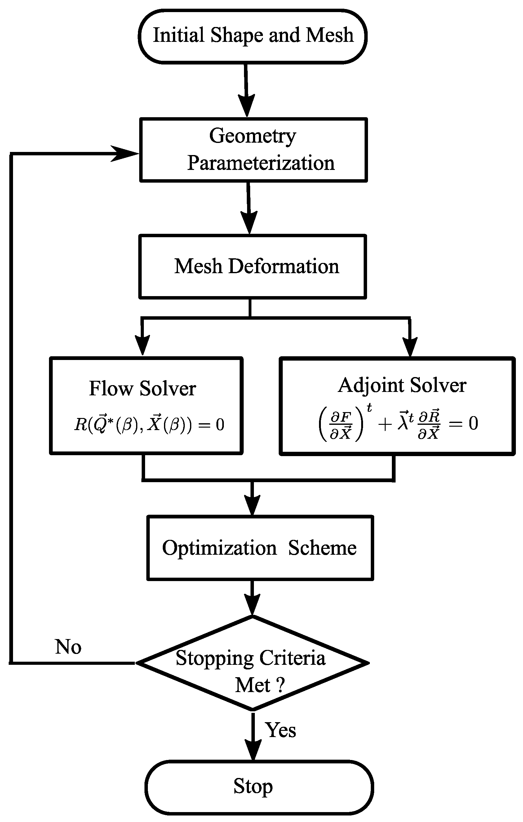
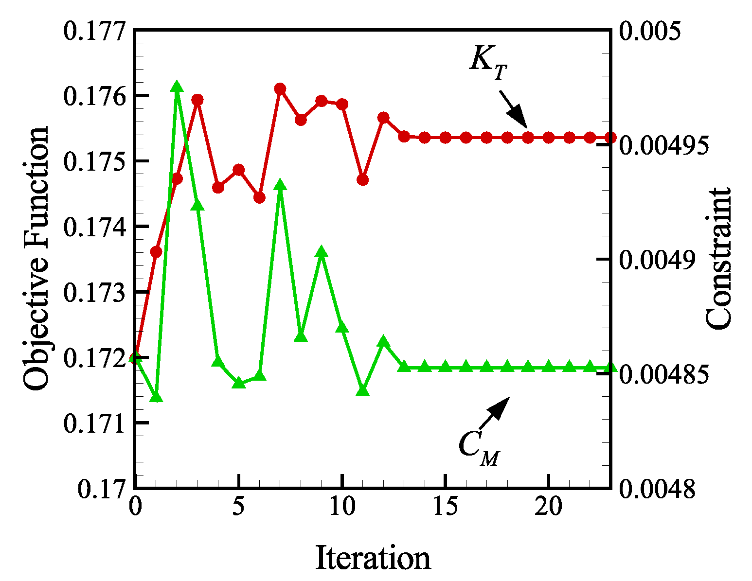
A common cost function under a aerodynamic optimization issue can be expressed as:

$$F=F(\overrightarrow{Q^{*}}(\overrightarrow{\beta }),\overrightarrow{X}(\overrightarrow{\beta }))$$

(21)

where F is the aerodynamic coefficients, which, generally, can be obtained by integration over the computing mesh. $\overrightarrow{Q^{*}}$ is the vector of conservative variables for a steady converged solution. $\overrightarrow{X}$ and $\overrightarrow{\beta }$ are the vector of mesh coordinates and matrix of design variables. Obviously, the variables $\overrightarrow{Q^{*}}$ and $\overrightarrow{X}$ are related to the design variables $\overrightarrow{\beta }$ explicitly. The sensitivity derivative is:

$$\frac{dF}{d{\beta }_k}={\left(\frac{\partial F}{\partial \overrightarrow{Q}}\right)}^t\frac{d\overrightarrow{Q^{*}}}{d{\beta }_k}+{\left(\frac{\partial F}{\partial \overrightarrow{X}}\right)}^t\frac{d\overrightarrow{X}}{d{\beta }_k}$$

(22)

The derivatives $\partial F/\partial \overrightarrow{Q}$ and $\partial F/\partial \overrightarrow{X}$ can be obtained directly via the derivatives of the numerical integral form of $\overrightarrow{F}$. If considering the residual of steady converged equations, viz.:

$$R(\overrightarrow{Q^{*}}(\beta ),\overrightarrow{X}(\beta ))=0$$

(23)

If expressing the aerodynamic optimization by optimal control problem, the best value of the cost function in the dynamic system comes from a specific array of control variables vector $\overrightarrow{\beta }$, that is, the Equation (23) should be a constraint. Hence, the extremum of cost function is treated with method of Lagrange multipliers. Rewriting the Equation (22) by multiplying the multipliers:

$$\begin{array}{c}\hfill \frac{dF}{d{\beta }_k}={\left(\frac{\partial F}{\partial \overrightarrow{Q}}\right)}^t\frac{d\overrightarrow{Q^{*}}}{d{\beta }_k}+{\left(\frac{\partial F}{\partial \overrightarrow{X}}\right)}^t\frac{d\overrightarrow{X}}{d{\beta }_k}+{\overrightarrow{\lambda }}^t\left(\frac{\partial \overrightarrow{R}}{\partial \overrightarrow{Q}}\frac{d\overrightarrow{Q^{*}}}{d{\beta }_k}+\frac{\partial \overrightarrow{R}}{\partial \overrightarrow{X}}\frac{d\overrightarrow{X}}{d{\beta }_k}\right)\\ \hfill =\left[{\left(\frac{\partial F}{\partial \overrightarrow{Q}}\right)}^t+{\overrightarrow{\lambda }}^t\frac{\partial \overrightarrow{R}}{\partial \overrightarrow{Q}}\right]\frac{d\overrightarrow{Q^{*}}}{d{\beta }_k}+\left[{\left(\frac{\partial F}{\partial \overrightarrow{X}}\right)}^t+{\overrightarrow{\lambda }}^t\frac{\partial \overrightarrow{R}}{\partial \overrightarrow{X}}\right]\frac{d\overrightarrow{X}}{d{\beta }_k}\end{array}$$

(24)

where $\overrightarrow{\lambda }$ is the adjoint vector. If setting the term $\left[{\left(\frac{\partial F}{\partial \overrightarrow{Q}}\right)}^t+\overrightarrow{{\lambda }^t}\frac{\partial \overrightarrow{R}}{\partial \overrightarrow{Q}}\right]$ to be zero, $\overrightarrow{\lambda }$ is the only variable which need to be used for the derivatives of F to $\overrightarrow{\beta }$, viz.:

$$\frac{dF}{d{\beta }_k}=\left[{\left(\frac{\partial F}{\partial \overrightarrow{X}}\right)}^t+\overrightarrow{{\lambda }^t}\frac{\partial \overrightarrow{R}}{\partial \overrightarrow{X}}\right]\frac{d\overrightarrow{X}}{d{\beta }_k}$$

(25)

Under a rotation frame, the effect of Coriolis force and the centrifugal force is included into momentum equations. Meanwhile, the relative velocity $\overrightarrow{v_r}$ also appears in inviscous flux. The new residual matrix is written as:

$${\overrightarrow{R}}_i=-{\Sigma }_{face}\overrightarrow{F}({\overrightarrow{Q}}_i)·\overrightarrow{n}S-{\overrightarrow{S}}_i$$

(26)

where $\overrightarrow{F}({\overrightarrow{Q}}_i)$ is the flux term, and ${\overrightarrow{S}}_i$ is the complex source term of Coriolis and centrifugal forces.

The source term ${\overrightarrow{S}}_i$ stands for the Coriolis force, which is:

$${\overrightarrow{S}}_i={\left[\begin{array}{c}0\\ \rho (\overrightarrow{\Omega }\times \overrightarrow{V})\\ 0\end{array}\right]}_i={\left[\begin{array}{c}0\\ \rho ({\Omega }_{y}w-{\Omega }_{z}v)\\ \rho ({\Omega }_{z}u-{\Omega }_{x}w)\\ \rho ({\Omega }_{x}v-{\Omega }_{y}u)\\ 0\end{array}\right]}_i$$

(27)

and we can have:

$$\frac{\partial {\overrightarrow{S}}_i}{\partial {\overrightarrow{Q}}_i}={\left[\begin{array}{c}\frac{{\overrightarrow{S}}_i}{\partial \rho }\\ \frac{{\overrightarrow{S}}_i}{\partial \left(\rho u\right)}\\ \frac{{\overrightarrow{S}}_i}{\partial \left(\rho v\right)}\\ \frac{{\overrightarrow{S}}_i}{\partial \left(\rho w\right)}\end{array}\right]}_i={\left[\begin{array}{ccccc}0& 0& 0& 0& 0\\ 0& 0& {\Omega }_z& -{\Omega }_y& 0\\ 0& -{\Omega }_z& 0& {\Omega }_x& 0\\ 0& {\Omega }_y& -{\Omega }_x& 0& 0\\ 0& 0& 0& 0& 0\end{array}\right]}_i$$

(28)

The contribution of inviscous flux which contains the rotation source term to the original one can be recognized as the difference between inertial and non-inertial coordinates, if denoting the inertial inviscous flux with prime symbol, it gives:

$$\delta \overrightarrow{F}{(\overrightarrow{Q})}_i=-{\left[\begin{array}{c}\rho (\overrightarrow{\Omega }\times \overrightarrow{r}))\\ \rho \overrightarrow{u}\otimes (\rho (\overrightarrow{\Omega }\times \overrightarrow{r}))\\ \rho E(\rho (\overrightarrow{\Omega }\times \overrightarrow{r}))\end{array}\right]}_i=-(\overrightarrow{\Omega }\times \overrightarrow{r}){\left[\begin{array}{c}\rho \\ \rho u\\ \rho v\\ \rho w\\ \rho E\end{array}\right]}_i$$

(29)

The derivative of increment $\delta \overrightarrow{F}{(\overrightarrow{Q})}_i$ to the flow variables ${\overrightarrow{Q}}_i$ is:

$$\frac{\partial \Delta {\overrightarrow{F}}_i}{\partial {\overrightarrow{Q}}_i}=-(\overrightarrow{\Omega }\times \overrightarrow{r}){\left[\begin{array}{ccccc}1& 0& 0& 0& 0\\ 0& 1& 0& 0& 0\\ 0& 0& 1& 0& 0\\ 0& 0& 0& 1& 0\\ 0& 0& 0& 0& 1\end{array}\right]}_i$$

(30)

In order to make the Jacobi of the adjoint equations as same as those of the flow equations in numerical solving procedure, the adjoint equations needed to be written in augmented matrix [33]:

$${\left(\frac{\partial \Delta \overrightarrow{R}(\overrightarrow{Q^{*}})}{\partial \overrightarrow{Q}}\right)}^{t,n}\Delta \overrightarrow{\lambda }=-\left[\frac{\partial F}{\partial \overrightarrow{q}}+{\left(\frac{\partial \Delta \overrightarrow{R}(\overrightarrow{Q^{*}})}{\partial \overrightarrow{Q}}\right)}^{t,n}\overrightarrow{\lambda }\right]$$

(31)

where $\overrightarrow{{\lambda }^{n+1}}={\overrightarrow{\lambda }}^n{+}^n\Delta \overrightarrow{\lambda }$. The dominate part of Equation (31) is reserved in the right-hand of the above equation. The only requirement for the left-hand side is that the term ${}^n\Delta \overrightarrow{\lambda }$ could converged to zero. The diagonally dominant feature of the Equation (31) is obtained by adding the pseudo time term, which gives:

$${\left(\frac{\overrightarrow{I}}{\Delta t}\frac{\partial \Delta \overrightarrow{R}(\overrightarrow{Q^{*}})}{\partial \overrightarrow{Q}}\right)}^{t,n}\Delta \overrightarrow{\lambda }=-\left[\frac{\partial F}{\partial \overrightarrow{q}}+{\left(\frac{\partial \Delta \overrightarrow{R}(\overrightarrow{Q^{*}})}{\partial \overrightarrow{Q}}\right)}^{t,n}\overrightarrow{\lambda }\right]$$

(32)

Hence, the left-side of the above equation has the same structure with flow equations, the preconditioning approach can be used for flow and adjoint equations at the same time.

Optimization Scheme

For a optimized system, the mesh deformation, flow solver, and optimization scheme are linked together with the optimization framework which is shown in Figure 5. The optimization algorithm is Sequential Quadratic Programming (SQP) [34], which enables the solving of the optimal problem under explicit aerodynamic and geometric constraints, such as minimum lift, minimum volume, maximum pitching moment, and so on.

4. Results and Discussion

From perspective of engineering, notwithstanding, an optimization of propeller is a multidisciplinary issue in which the constraints and objects come from different disciplines, such as aerodynamics, structural strength, control, and so on. One of the most important targets of optimization of propeller, generally, is maximizing the thrust under specific torque from geometry deformation. In present work, the aerodynamic improvement will be used to achieve this goal. Three geometrical parameters are considered herein, which are the distribution of torsion angles, the profiles and chord length of the blade in control sections.

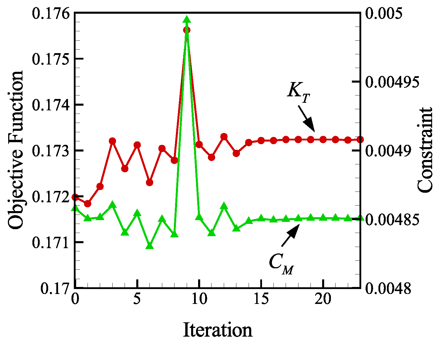
4.1. The Optimization of Twisted Angles Distribution

The FFD box for this task is demonstrated in Figure 6. The red points stand for the control points, meanwhile, 8 deforming slices are arranged and every y-slice are only permitted to displace in x–z plane. The thickness limit is not involved due to no thickness variation brought by this changing method. The optimization problem is stated mathematically as follows:

$$\begin{array}{cc}\hfill & max:K_T(\overrightarrow{\beta })\hfill \\ \hfill & Subjectto:\left\{\begin{array}{c}{C}_M\le {\left(C_M\right)}_0\hfill \\ {\beta }_k^l\le {\beta }_k\le {\beta }_k^u,k=1,\dots ,8\hfill \end{array}\right.\hfill \end{array}$$

(33)

where $\overrightarrow{\beta }$ is the vector of design variables which contains 8 ranges which the twisted angles can vary in, $K_T$ the thrust coefficient, $C_M$ the bending momentum coefficient of wing root, ${\beta }_l$ and ${\beta }_u$ denote for the lower and upper bounds of variation of design variables. It should be noted that $K_T$ and $C_M$ are positive, so a non-increasing $C_M$ (i.e., smaller than the initial bending momentum $C_{M0}$) is regarded as a constraint. In Figure 7, the history of variation of cost and constraint functions are plotted. After 15 iterations, the converged condition is achieved. $K_T$ is improved by a value of 0.95% with a roughly non-increasing $C_M$. If observing from the downwind side (i.e., View A), as shown in Figure 8, the $C_p$ that closes to the root of the blade shows more low-pressure region in optimized configuration, when compared with the results of baseline. An opposite variation, however, is demonstrated in Figure 9, which comes from the observation from upwind side (i.e., View B). The aerodynamic load, hence, moves toward the blade tip.

The twisted angles near the root of the blade are decreased with an obvious drop of the peak of the negative pressure, which is demonstrated in Figure 10b. The middle plane (i.e., y/b = 50%) gives a similar change but with a smaller decreasing torsion angles. At the tip location, the optimizer slightly increases the twisted angle with the strengthening of a negative pressure peak. The propeller thrust is mainly determined by the local profile and line velocity, and the line velocity at the root is relatively smaller than that at the tip. Hence, the thrust coefficient $\eta$ improved accordingly with a little increase twisted angle at the tip, as demonstrated in

Table 2. Design result with varying the distribution of twisted angles.

	${\mathit{K}}_{\mathit{T}}$	${\mathit{C}}_{\mathit{M}}$	$\mathit{\eta }$
Baseline	0.17197	0.00486	0.50685
Optimized	0.17324	0.00485	0.51165
Increment	0.74%	−0.21%	0.95%

. The reason why a corresponding decrease at the root is to reduce the pressure drag of the propeller.

4.2. The Optimization of Chord Length Distribution

The distribution of the chord length of the blade affects the cross flow, i.e., the three-dimensional effect, on the surface. The FFD box used in this case, shown in Figure 11, is the same as the above one. The control points are limited only to move along the direction, which is parallel with the chord line. In total, there are 32 control points which are arranged in 8 control planes. The cost function and constraint used here is the same as the Equation (33). The optimized history is shown in Figure 12. As shown in Figure 13 and Figure 14, the radian of the leading edge of the blade is decreased, and hence pressure near the trailing edge is enhanced. Correspondingly, the trailing edge of the blade is extended for generating enough lift. This behavior is demonstrated in Figure 15 by the geometrical change. The negative peak of the pressure lifts at the root and depressed at the tip, and this operation will reduce the cross-flow due to a straight line in the leading edge of the blade, single decrease the magnitude the wing-tip vortex to some extent. Results in

Table 3. Design result with varying the distribution of chord length.

	${\mathit{K}}_{\mathit{T}}$	${\mathit{C}}_{\mathit{M}}$	$\mathit{\eta }$
Baseline	0.17197	0.00486	0.50685
Optimized	0.17536	0.00485	0.51791
Increment	1.97%	−0.21%	2.18%

has shown that the thrust coefficient is improved by 2.18%, corresponding to the same increment of bending moment with the above section.

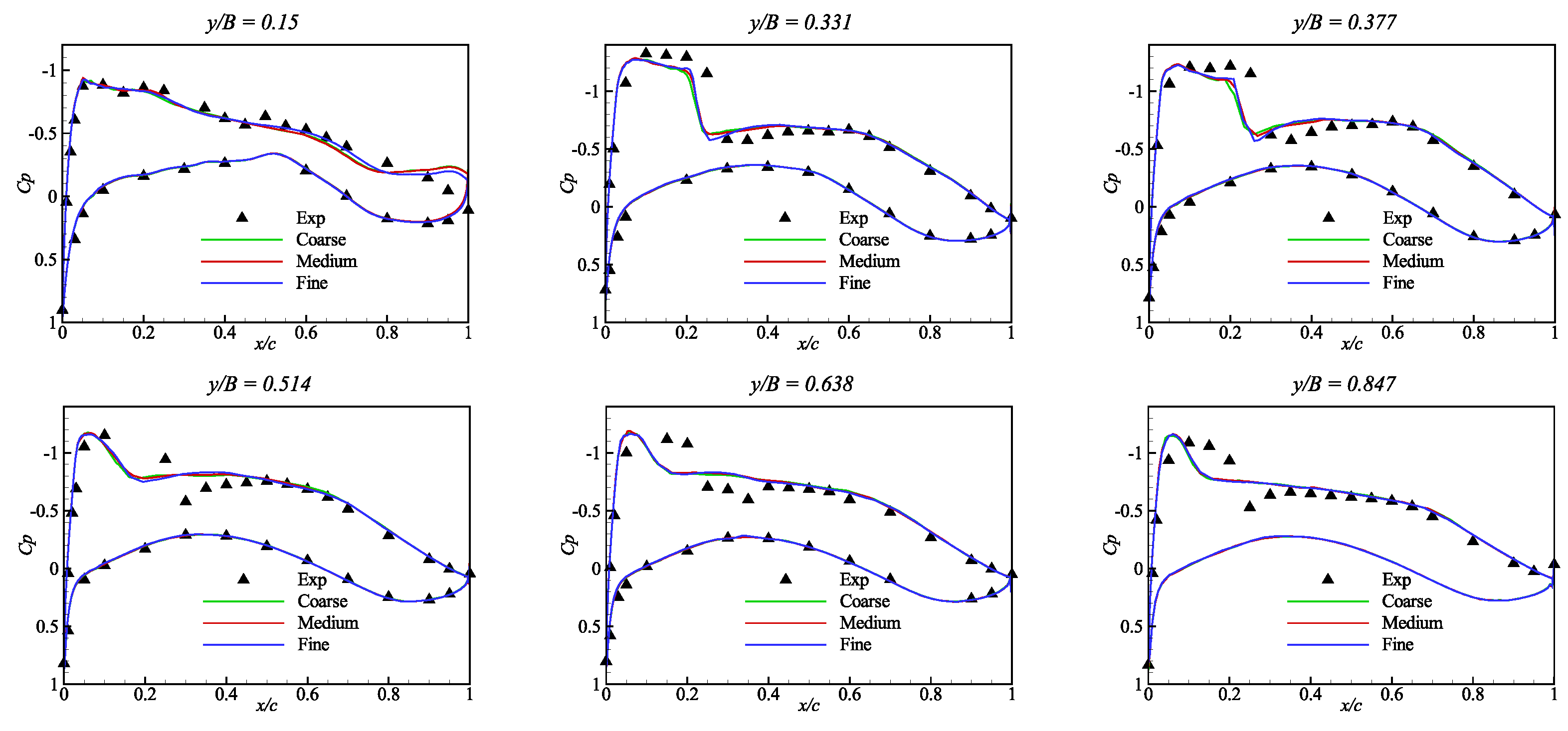
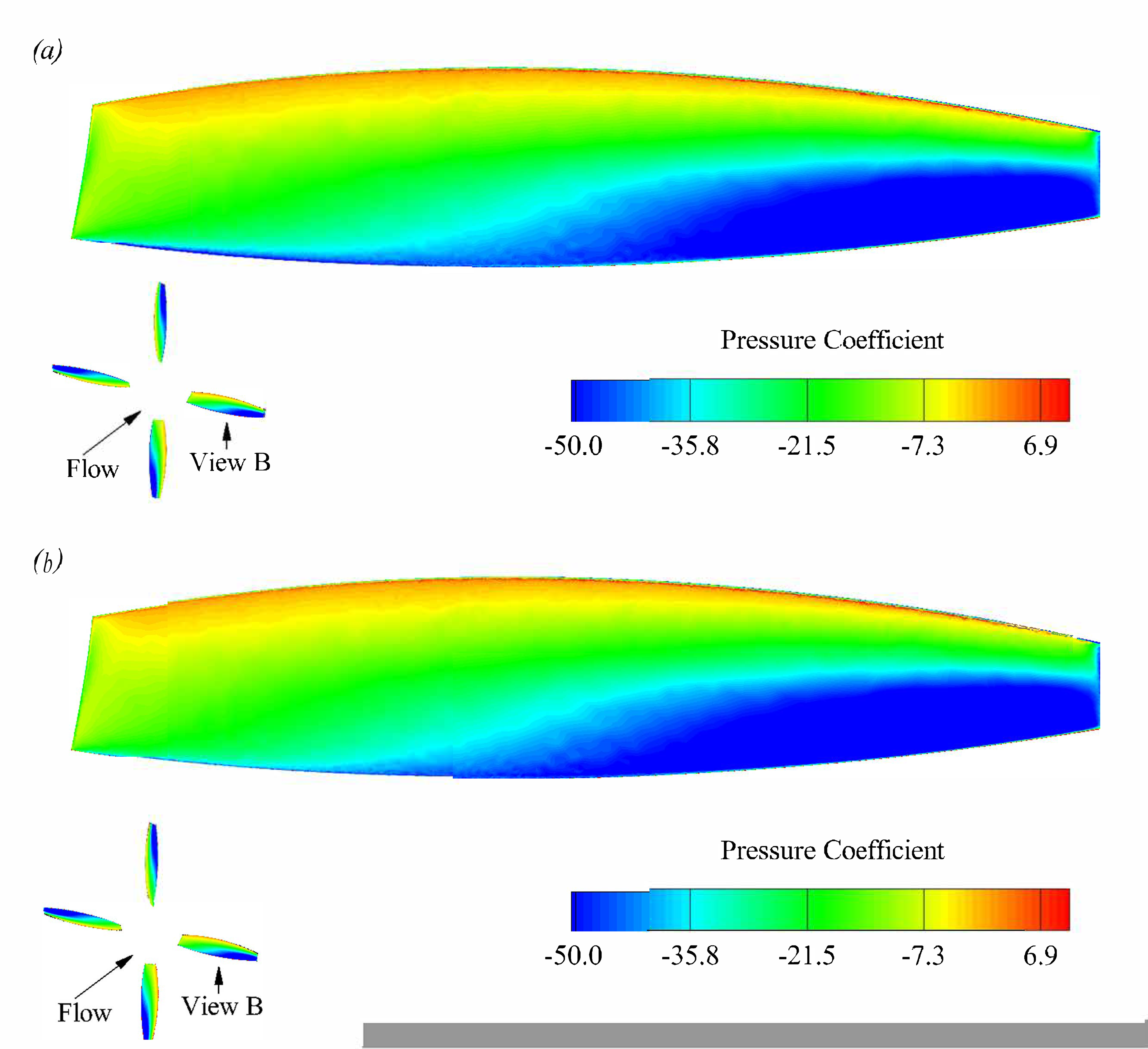
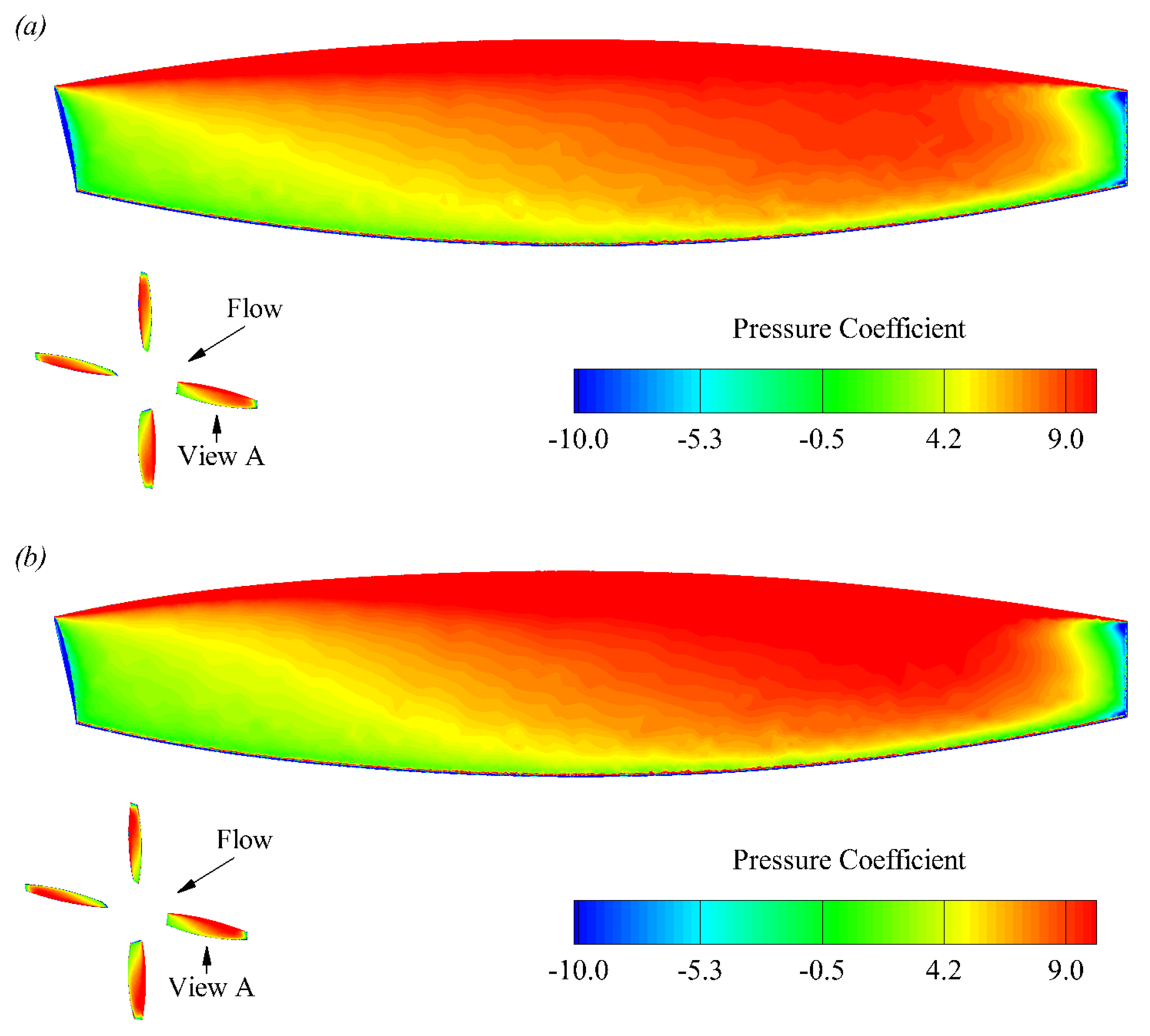
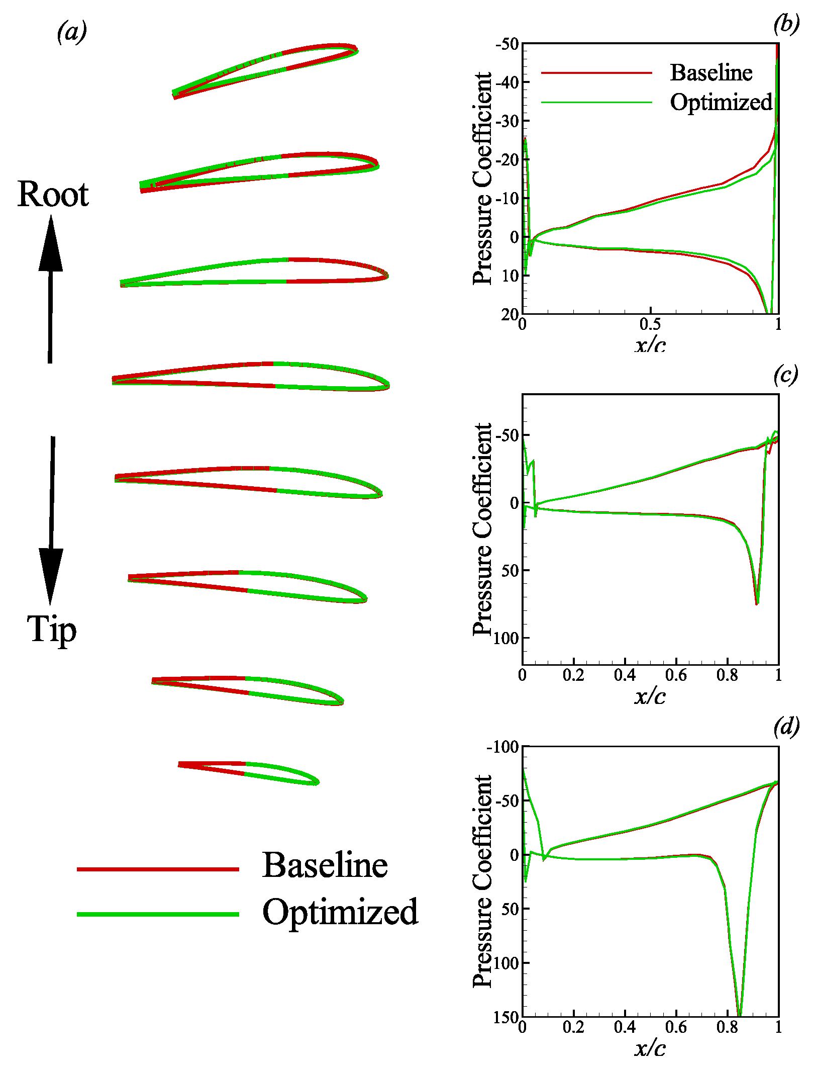
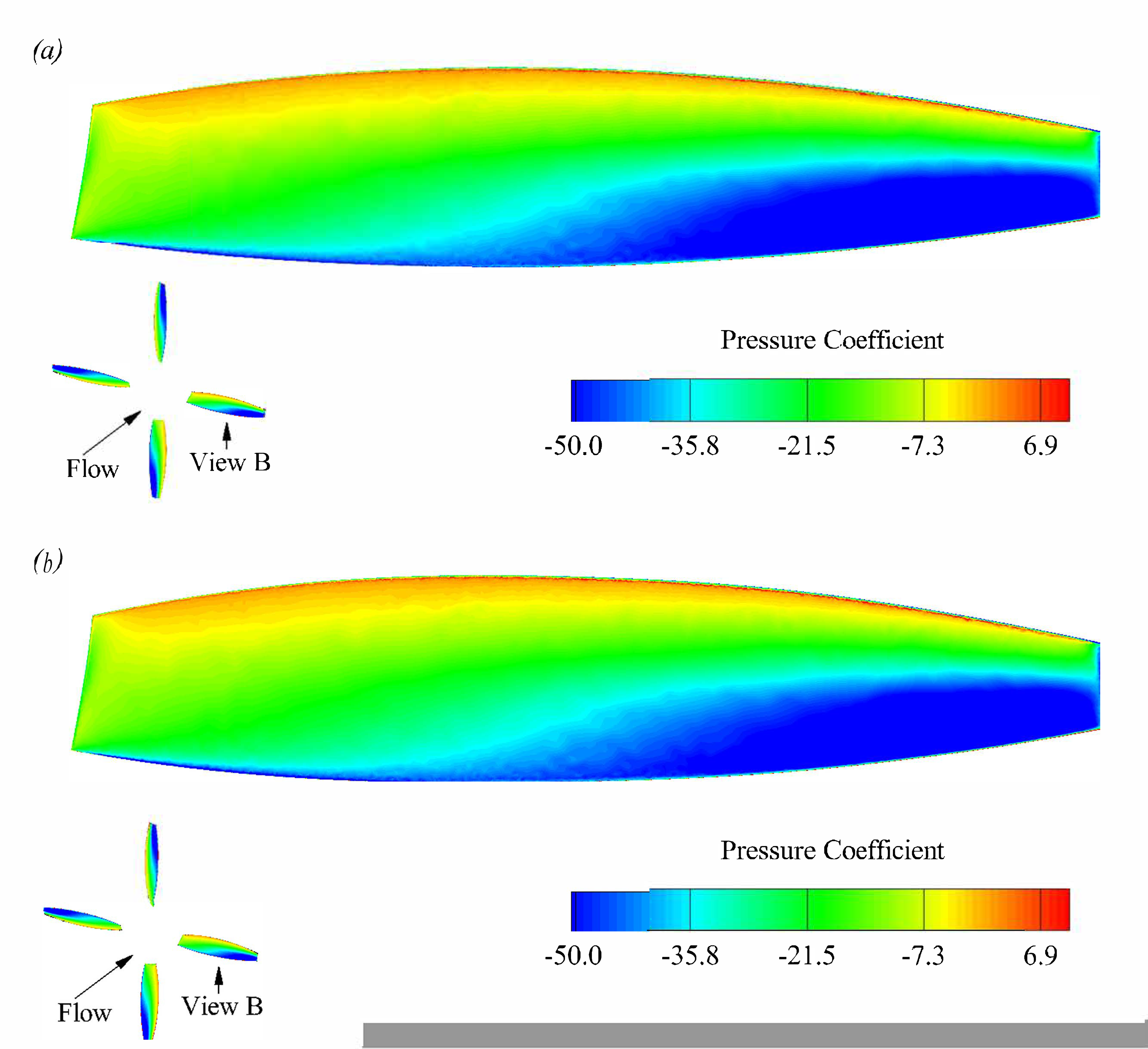
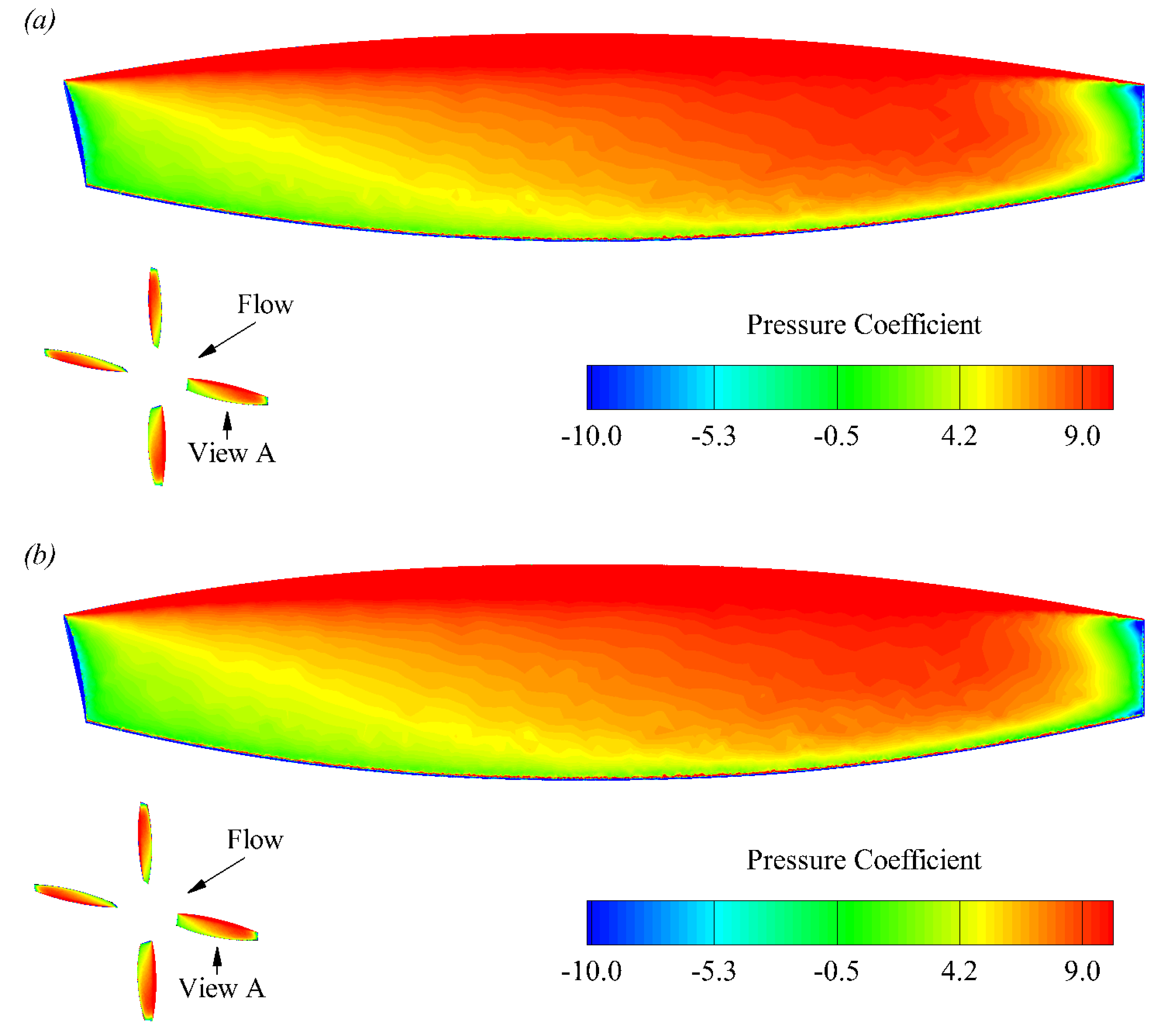
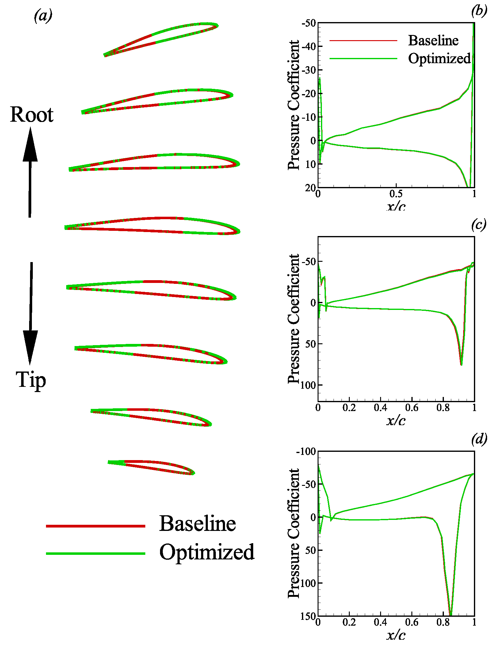
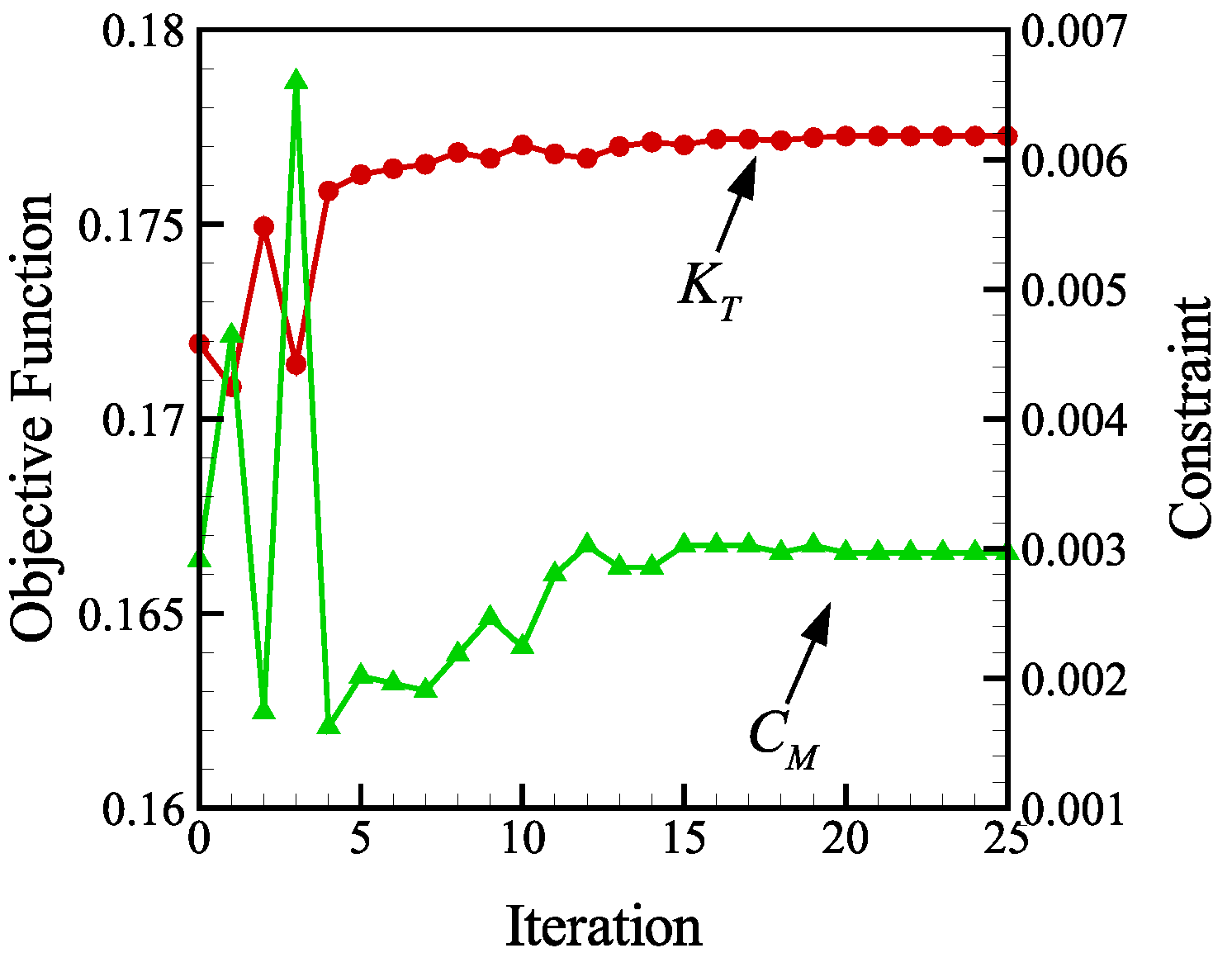
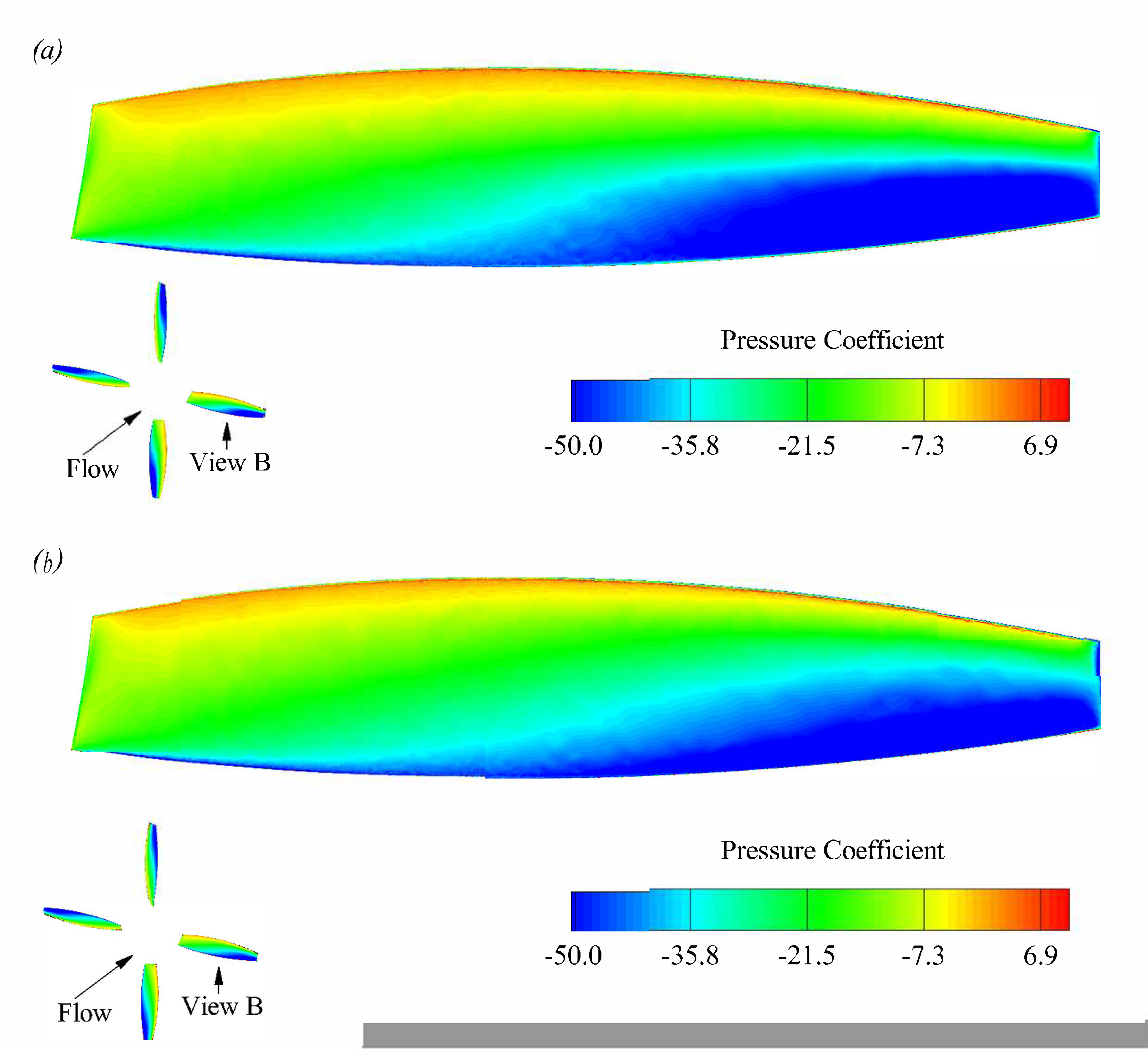
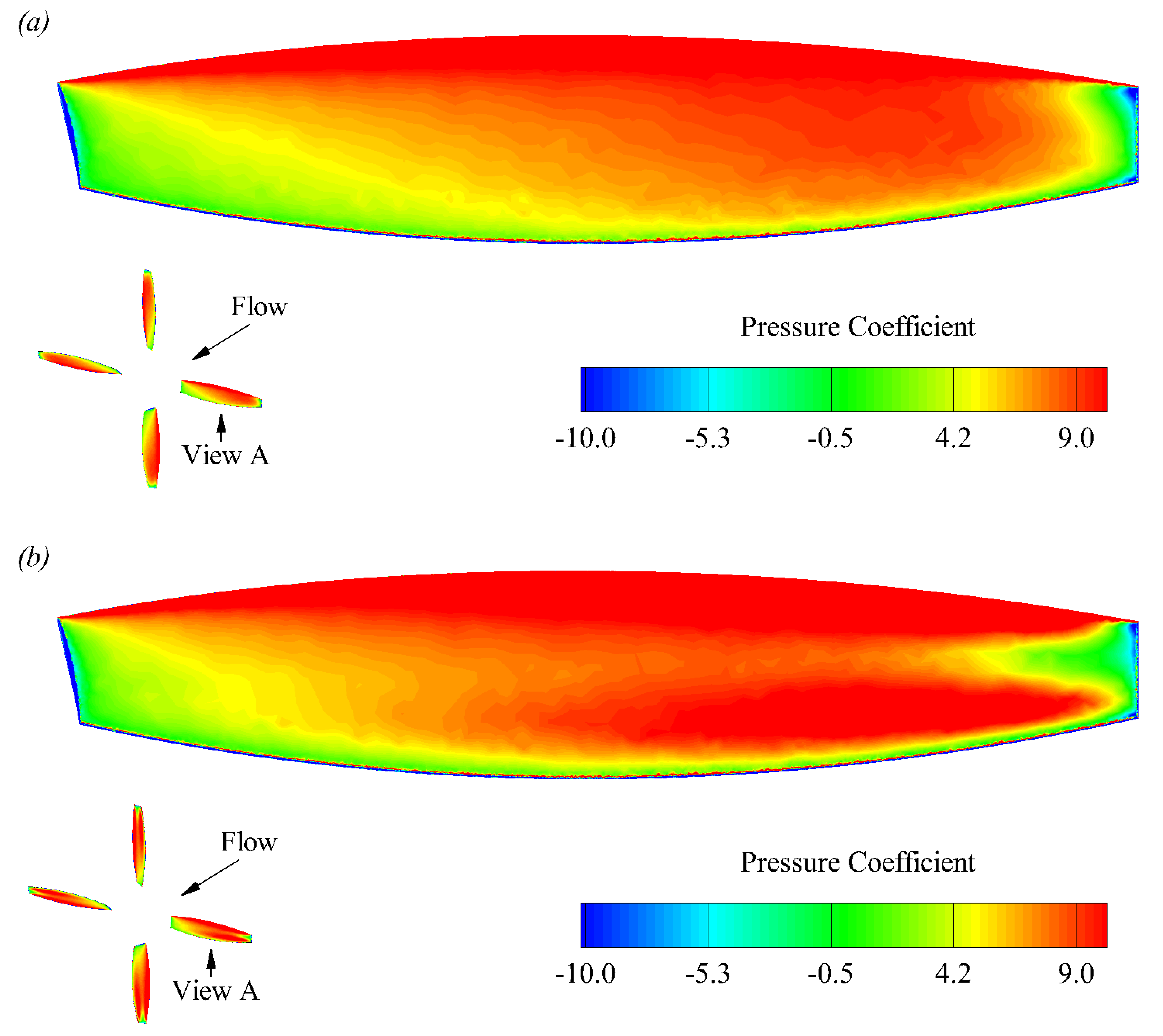
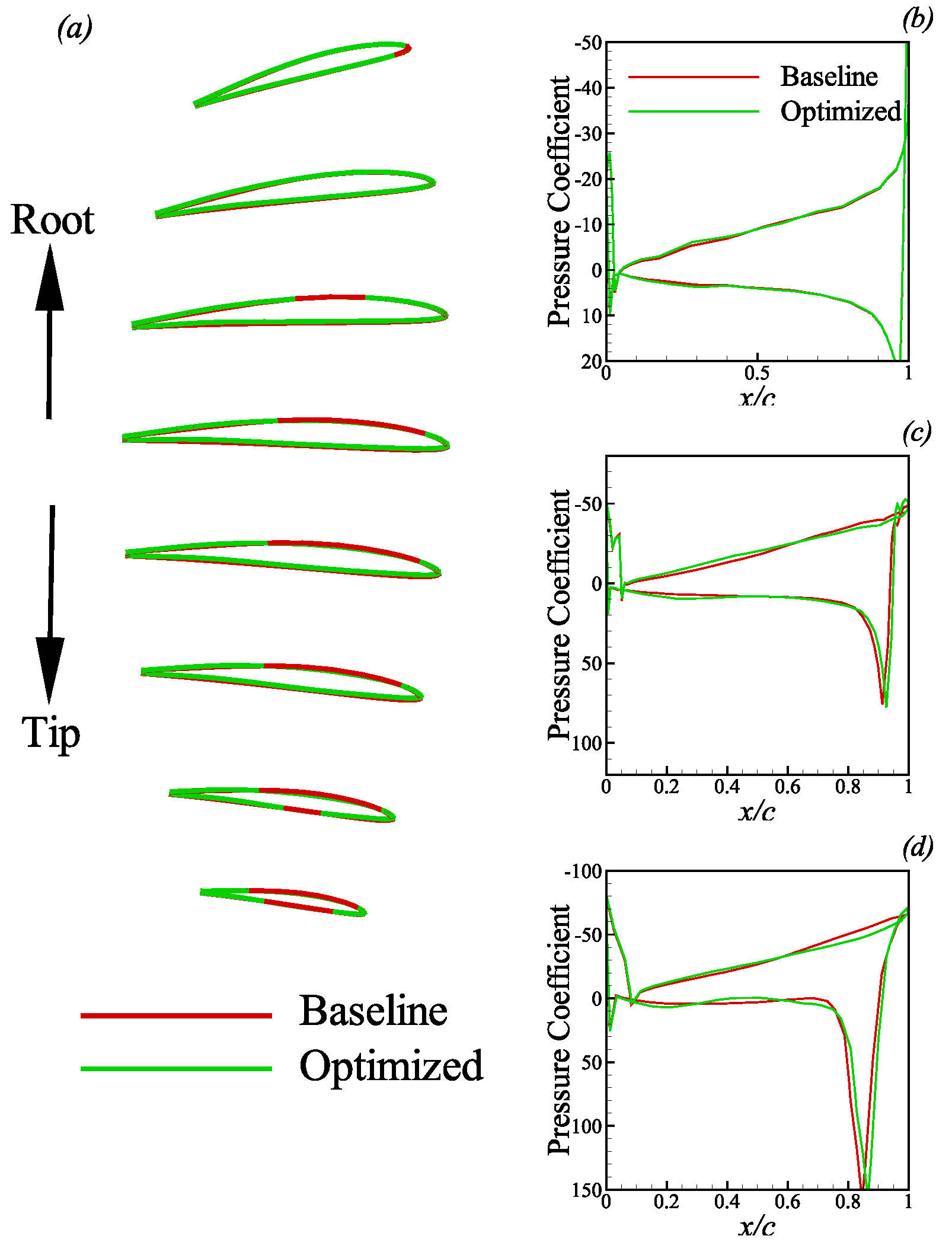
4.3. The Optimization of Profiles of Blade

The profiles of blade play a very important role in the aerodynamic devices. The control box is same with that used in the above case. The normal vector of every control plane is set to be vertical to the chord length of the profile. In total, 112 control points are used for the geometrical deformation. The optimized problem is illustrated as:

$$\begin{array}{cc}\hfill & max:K_T(\overrightarrow{\beta })\hfill \\ \hfill & Subjectto:\left\{\begin{array}{c}{C}_M\le {\left(C_M\right)}_0\hfill \\ t_i\ge {\left(t_i\right)}_0\hfill \\ {\beta }_k^l\le {\beta }_k\le {\beta }_k^u,k=1,\dots ,8\hfill \end{array}\right.\hfill \end{array}$$

(34)

where $t_i$ denotes the thickness of the profile in the i control plane. The design variables $\overrightarrow{\beta }$ in the present case are used to generate the fluctuating displacement in the local control plane. The optimization achieved convergence after the 13th iteration as shown in Figure 16. From the value demonstrated in

Table 4. Design result with varying the airfoil profiles.

	${\mathit{K}}_{\mathit{T}}$	${\mathit{C}}_{\mathit{M}}$	$\mathit{\eta }$
Baseline	0.17197	0.00486	0.50685
Optimized	0.17725	0.00485	0.52349
Increment	3.07%	−0.21%	3.28%

, the thrust coefficient is improved by 3.28%. As shown in Figure 17, the high pressure region extends to the trailing edge of the blade after optimization. At the upwind surface, the low-pressure region is compressed towards the leading edge, which is shown in Figure 18. From the comparison between the variation of geometry from baseline to optimization. The negative peak of pressure near the tip direction is decreased with reduction of head radius of the profile. Meanwhile, most of profiles show that the camber are increased to obtain a higher wing load, which will lift the thrust up dramatically. From the Figure 19, the lower sides of the profiles is modified to be more flat, namely, a relatively high positive pressure will be kept.

5. Conclusions

Shape optimizations for several isolated rotors in propeller have been performed in present paper. The adjoint equations are solved with the Navier–Stokes equations at the same time. A wing-body configuration was used to validate the basic solver. The rotating effect of the propeller is considered here by using MRF method, which can improve the design accuracy and efficiency. Correspondingly, a propeller with medium Reynolds number calculated by MRF method, and three indicators of performance of propeller were predicted reasonably. In present study, the optimization was conducted to maximize the thrust coefficient $K_T$ based on gradient solver. The constraint was a non-increasing torsional momentum of wing-root. Three parameters were selected herein to demonstrate the influence of the distribution of twisted angles, the chord length and airfoil of the blades. As a first parameter, the twist distribution was studied and the results demonstrated a local optimum in agreement with the common knowledge that high twisted angles lead to high wing loads. The second case, which changed the contour line of both leading and trailing edges of the blade, improved the performance of the propeller by reducing the cross-flow. The last case was devised to optimize the profiles of the blade. The optimum shape presents a 3.28% enhancement of thrust efficiency by changing the profiles.

References

1. Wald, Q. The Wright Brothers propeller theory and design. In Proceedings of the 37th Joint Propulsion Conference and Exhibit, Salt Lake City, UT, USA, 8–11 July 2001; p. 3386. [Google Scholar]
2. Hicks, R.M.; Murman, E.M.; Vanderplaats, G.N. An Assessment of Airfoil Design by Numerical Optimization; National Aeronautics and Space Administration: Washington, DC, USA, 1974.
3. Vanderplaats, G.N.; Hicks, R.M.; Murman, E.M. Application of numerical optimization techniques to airfoil design. In Proceedings of the NASA Conference on Aerodynamic Analysis Requiring Advanced Computers, Hampton, VA, USA, 4–6 May 1975; pp. 749–768. [Google Scholar]
4. Pironneau, O. Optimal shape design for elliptic systems. In System Modeling and Optimization; Springer: Berlin, Germany, 1982; pp. 42–66. [Google Scholar]
5. Jameson, A.; Baker, T. Solution of the Euler equations for complex configurations. In Proceedings of the 6th Computational Fluid Dynamics Conference Danvers, Danvers, MA, USA, 13–15 July 1983; p. 1929. [Google Scholar]
6. Jameson, A. Optimum aerodynamic design using CFD and control theory. In Proceedings of the 12th Computational Fluid Dynamics Conference, San Diego, CA, USA, 19–22 June 1995; p. 1729. [Google Scholar]
7. Jameson, A.; Martinelli, L.; Pierce, N. Optimum aerodynamic design using the Navier–Stokes equations. Theor. Comput. Fluid Dyn. 1998, 10, 213–237. [Google Scholar] [CrossRef] [Green Version]
8. Jameson, A.; Martinelli, L. Aerodynamic shape optimization techniques based on control theory. In Computational Mathematics Driven by Industrial Problems; Springer: Berlin, Germany, 2000; pp. 151–221. [Google Scholar]
9. Lerbs, H.W. Moderately Loaded Propellers with a Finite Number of Blades and a Arbitrary Distribution of Circulations. Trans. Sname 1952, 60, 73–123. [Google Scholar]
10. Kerwin, J.E. The Solution of Propeller Lifting Surface Problems by Vortex Lattice Methods; Technical Report; Massachusetts Institute of Technology Cambridge, Department of Naval Architecture and Marine: Cambridge, MA, USA, 1961. [Google Scholar]
11. Morgan, W.B.; Silovic, V.; Denny, S.B. Propeller Lifting-Surface Corrections; Technical Report; Hydro-and Aerodynamics Lab Lyngby (Denmark) Hydrodynamics Section: Copenhagen, Denmark, 1968. [Google Scholar]
12. Denny, S.B. Cavitation and Open-Water Performance Tests of a Series of Propellers Designed by Lifting-Surface Methods; Technical Report; David W. Taylor Naval Ship Research and Development Center Bethesda MD Department: Bethesda, MD, USA, 1968. [Google Scholar]
13. Chausee, D. Computation of Three-Dimensional Flow through Prop Fans; NEAR TR-199; Nielsen Engineering and Research Inc.: Santa Clara, CA, USA, 1979. [Google Scholar]
14. Hess, J.L.; Valarezo, W.O. Calculation of steady flow about propellers using a surface panel method. J. Propuls. Power 1985, 1, 470–476. [Google Scholar] [CrossRef]
15. Hanson, D.B. Compressible lifting surface theory for propeller performance calculation. J. Aircr. 1985, 22, 19–27. [Google Scholar] [CrossRef]
16. Xiang, S.; Qiang, L.Y.; Tong, G.; Zhao, P.W.; Tong, X.S.; Dong, L.Y. An improved propeller design method for the electric aircraft. Aerosp. Sci. Technol. 2018, 78, 488–493. [Google Scholar] [CrossRef]
17. Alba, C.; Elham, A.; German, B.J.; Veldhuis, L.L. A surrogate-based multi-disciplinary design optimization framework modeling wing–propeller interaction. Aerosp. Sci. Technol. 2018, 78, 721–733. [Google Scholar] [CrossRef]
18. Zheng, X.k.; Wang, X.l.; Cheng, Z.j.; Han, D. The efficiency analysis of high-altitude propeller based on vortex lattice lifting line theory. Aeronaut. J. 2017, 121, 141–162. [Google Scholar] [CrossRef]
19. Allen, C.; Rendall, S.T.; Morris, A. Computational-fluid-dynamics-based twist optimization of hovering rotors. J. Aircr. 2010, 47, 2075–2085. [Google Scholar] [CrossRef]
20. Dumont, A.; Le Pape, A.; Peter, J.; Huberson, S. Aerodynamic shape optimization of hovering rotors using a discrete adjoint of the Reynolds-Averaged Navier–Stokes Equations. J. Am. Helicopter Soc. 2011, 56, 1–11. [Google Scholar] [CrossRef]
21. Allen, C.B.; Rendall, T.C. CFD-based optimization of hovering rotors using radial basis functions for shape parameterization and mesh deformation. Optim. Eng. 2013, 14, 97–118. [Google Scholar] [CrossRef]
22. Farrokhfal, H.; Pishevar, A. Aerodynamic shape optimization of hovering rotor blades using a coupled free wake—CFD and adjoint method. Aerosp. Sci. Technol. 2013, 28, 21–30. [Google Scholar] [CrossRef]
23. Dhert, T.; Ashuri, T.; Martins, J.R. Aerodynamic shape optimization of wind turbine blades using a Reynolds-averaged Navier–Stokes model and an adjoint method. Wind. Energy 2017, 20, 909–926. [Google Scholar] [CrossRef]
24. Roe, P.L. Approximate Riemann solvers, parameter vectors, and difference schemes. J. Comput. Phys. 1981, 43, 357–372. [Google Scholar] [CrossRef]
25. Colella, P. A direct Eulerian MUSCL scheme for gas dynamics. Siam J. Sci. Stat. Comput. 1985, 6, 104–117. [Google Scholar] [CrossRef] [Green Version]
26. Venkatakrishnan, V. Convergence to steady state solutions of the Euler equations on unstructured grids with limiters. J. Comput. Phys. 1995, 118, 120–130. [Google Scholar] [CrossRef]
27. Spalart, P.; Allmaras, S. A one-equation turbulence model for aerodynamic flows. In Proceedings of the 30th Aerospace Sciences Meeting and Exhibit, Reno, NV, USA, 6–9 January 1992; p. 439. [Google Scholar]
28. Nielsen, E.J.; Lu, J.; Park, M.A.; Darmofal, D.L. An implicit, exact dual adjoint solution method for turbulent flows on unstructured grids. Comput. Fluids 2004, 33, 1131–1155. [Google Scholar] [CrossRef]
29. Rumsey, C.L.; Rivers, S.M.; Morrison, J.H. Study of CFD variation on transport configurations from the second drag-prediction workshop. Comput. Fluids 2005, 34, 785–816. [Google Scholar] [CrossRef]
30. Samareh, J.A. Novel multidisciplinary shape parameterization approach. J. Aircr. 2001, 38, 1015–1024. [Google Scholar] [CrossRef]
31. Saad, Y.; Schultz, M.H. GMRES: A generalized minimal residual algorithm for solving nonsymmetric linear systems. Siam J. Sci. Stat. Comput. 1986, 7, 856–869. [Google Scholar] [CrossRef] [Green Version]
32. Ghoddoussi, A. A more Comprehensive Database for Propeller Performance Validations at Low Reynolds Numbers. Ph.D. Thesis, Wichita State University, Wichita, KS, USA, 2016. [Google Scholar]
33. Mavriplis, D.J. Discrete adjoint-based approach for optimization problems on three-dimensional unstructured meshes. AIAA J. 2007, 45, 741–750. [Google Scholar] [CrossRef] [Green Version]
34. Boggs, P.T.; Tolle, J.W. Sequential quadratic programming. Acta Numer. 1995, 4, 1–51. [Google Scholar] [CrossRef]
Figure 1. Comparison of pressure distribution for different meshes.
Energies 15 08588 g001
Figure 2. An example of the FFD technique applied to the 3D wing deformation.
Energies 15 08588 g002
Figure 3. The mesh for the propeller. (a) The mesh detail on the propeller hub. (b) The rotating region around the propeller. (c) The surface mesh of propeller.
Energies 15 08588 g003
Figure 4. Comparison of characteristic parameters of propeller with different methods ((a): pressure coefficient, (b): torque coefficient, (c): propeller efficiency).
Energies 15 08588 g004
Figure 5. Flowchart of the optimization process.
Energies 15 08588 g005
Figure 6. The FFD box used for torsion deformation of one blade.
Energies 15 08588 g006
Figure 7. Optimization history with torsion angles as design variables.
Energies 15 08588 g007
Figure 8. The effect of changing twist angles of profiles on pressure coefficient contour from View A: (a) Baseline; (b) Optimized.
Energies 15 08588 g008
Figure 9. The effect of changing twist angles of profiles on pressure coefficient contour from View B: (a) Baseline; (b) Optimized.
Energies 15 08588 g009
Figure 10. Comparison of variation of geometry and pressure coefficient from baseline and optimized profiles by changing twist angles. (a) Twisted angles. Pressure coefficient at (b) y/B = 5%, (c) y/B = 50% and (d) y/B = 90%.
Energies 15 08588 g010
Figure 11. The FFD box used for profiles deformation of one blade.
Energies 15 08588 g011
Figure 12. Optimization history with changing the chord length as design condition.
Energies 15 08588 g012
Figure 13. The effect of changing chord length of profiles on pressure coefficient contour from View A: (a) Baseline; (b) Optimized.
Energies 15 08588 g013
Figure 14. The effect of changing chord length of profiles on pressure coefficient contour from View B: (a) Baseline; (b) Optimized.
Energies 15 08588 g014
Figure 15. Comparison of variation of geometry and pressure coefficient from baseline and optimized profiles with changing the chord length of profiles. (a) Torsion angles. Pressure coefficient at (b) y/B = 5%, (c) y/B = 50% and (d) y/B = 90%.
Energies 15 08588 g015
Figure 16. Optimization history with blade profiles deformation as design condition.
Energies 15 08588 g016
Figure 17. The effect of changing profiles of blades on pressure coefficient contour from View A: (a) Baseline; (b) Optimized.
Energies 15 08588 g017
Figure 18. The effect of changing profiles of blades on pressure coefficient contour from View B: (a) Baseline; (b) Optimized.
Energies 15 08588 g018
Figure 19. Comparison of variation of blade profiles and pressure coefficient from baseline and optimized models. (a) Torsion angles. Pressure coefficient at (b) y/B = 5%, (c) y/B = 50% and (d) y/B = 90%.
Energies 15 08588 g019