Article

Numerical Study on Transverse Jet Mixing Enhanced by High Frequency Energy Deposition

1
School of Air and Missile Defense, Air Force Engineering University, Xi’an 710051, China
2
Hypervelocity Aerodynamics Institute, China Aerodynamics Research and Development Center, Mianyang 621000, China
3
Laboratory of Aerodynamics in Multiple Flow Regimes, China Aerodynamics Research and Development Center, Mianyang 621000, China
4
College of Electronics and Information, Darmstadt University of Technology, 65527 Darmstadt, Germany
*
Author to whom correspondence should be addressed.
Energies 2022, 15(21), 8264; https://doi.org/10.3390/en15218264
Submission received: 15 September 2022 / Revised: 9 October 2022 / Accepted: 10 October 2022 / Published: 4 November 2022

Abstract

:
Supersonic incoming flow has a large momentum, which makes it difficult for transverse jets to have a large penetration depth due to the strong compression of the incoming flow. This impacts the mixing efficiency of the jet in the supersonic combustor. This paper proposes a method to improve the mixing efficiency of a rectangular flow field model using pulsed energy deposition, which is verified numerically. In the simulations, the Navier–Stokes equations with an energy source are solved to simulate the effects of energy deposition with various distributions on the fuel mixture. The results show that the energy deposition increases the turbulent kinetic energy, which enlarges the scale of the flow vortex and improves the fuel mixing performance. The energy deposition is distributed upstream and significantly improves the mixing performance. Energy deposition can improve the penetration depth of fuel, which is more significant when the energy deposition is distributed downstream of the jet orifice. The energy deposition also slightly reduces the total pressure recovery coefficient. In general, an energy deposition that is distributed upstream of the jet has the best effect on the mixing efficiency.

1. Introduction

Scramjets are the core propulsion device to achieve fast and precise strikes worldwide and low-Earth-orbit space transportation and other important carriers. When the flight Mach number is greater than 5, this type of aircraft shows excellent cruise performance. Reliable fuel ignition and stable combustion is an important key technology in scramjet designs under hypersonic incoming flows. The effective time of supersonic airflow through the scramjet is at the millisecond scale, making it challenging to achieve fuel fragmentation, atomization, mixing, ignition, and flame stabilization.
Researchers have conducted extensive research on potential ways to improve the fuel mixing efficiency by employing active and passive flow control techniques inside a supersonic combustor. This includes various kinds of struts, steps, pulsed jets, cavities, aerodynamic ramps, pylons, transverse injectors, and cantilevered ramp injectors [1,2,3,4,5]. The application of their combinations has also attracted widespread attention. One popular technique to improve the mixing efficiency is to introduce streamwise vortexes into the flow. This promotes momentum exchange between the fuel and main flow while also increasing the penetration depth of the fuel [6,7,8,9]. However, the combination of traditional passive mixing enhancements and transverse jet flow makes it difficult to attain a sufficient mixing effect in supersonic flow. In addition, this method brings a total pressure loss to the scramjet.
The high Mach flow in modern scramjet combustors has a large dynamic pressure load. The complex flow field structure, such as the shock wave, separation zone, and return zone induced by the transverse jet and mainstream interference gives the flow field in the combustor with multi-scale, unsteady, and wide frequency bandwidth characteristics. Some active flow control techniques, such as the Helmholtz resonator, have difficulty matching the characteristics of the flow field. The above discussion indicates that new methods are urgently needed to maintain stable and efficient mixing in scramjets while causing minimal impact to the flow field.
In early studies, plasma was generated by DC glow/arc discharge in a closed chamber or in the form of a reverse jet that covers the surface of the experimental model. This is similar to the high-temperature plasma sheath produced by the spacecraft head during reentry. Due to the high energy consumption required to generate such global high-temperature plasma, the international community has gradually turned to using local, unsteady, etc. plasma to complete flow control. Plasma energy deposition, as one of the active flow control methods, is promising and has aroused widespread interest in recent years. Energy depositions can be realized from a variety of discharges, including pulsed (known as nanosecond/microsecond pulsed) or steady (known as quasi-direct current). These discharges are characterized by quick response times, high intensities, and wide frequency bandwidths. Their operating states can be flexibly adjusted based on the incoming flow conditions. As actuators based on energy deposition generally do not intrude on the flow, a large total pressure loss can be avoided, which may be caused by intrusive mechanical devices.
Leonov et al. [10] used high-resolution imaging to capture the evolution process of a quasi-DC discharge plasma energy deposition in high-speed flows. Their experimental results demonstrated that the extremely-fast turbulent expansion induced by discharge positively contributes to the mixing of non-premixed multi-component flows. Leonov et al. [11,12] also studied the effect of quasi-DC discharge on fuel mixing in supersonic combustors with a cavity. The oblique shock wave as induced by the thermal choking effect of discharge not only enhances fuel mixing in the shear layer but also increases the pressure in the cavity, which contributes to fuel combustion. Leonov et al. [11] studied the influence of quasi-DC discharge on supersonic combustors and used TDLAS absorption spectroscopy to measure the temperature and H2O concentration in the combustion area. The interactions between the plasma and fuel help form active regions downstream of the fuel injection and significantly increase the wall pressure. In 2013, Matsubara et al. [13] integrated a plasma torch and an insulating column discharge DBD to ignite the hydrogen jet in supersonic inflow and achieved successful ignition. The experimental results show that when the plasma torch is P = 3.8 kW, the wall pressure of the combustor is the same as that of the DBD plasma combined with P = 2.4 kW, and the DBD discharge power is only 8 W, which greatly conserves power consumption. Thus, the energy deposition is more effective in mixing enhancements when it is inside the jet. Ombrello et al. [14] experimentally studied the interactions between a pulsed discharge and a supersonic jet and found that the position of the discharge actuator has a considerable effect on the jet mixing and that there is an optimal actuation position. Fabian et al. [15] studied the effects of laser energy depositions on the mixing in a supersonic combustor. It is concluded that the energy depositions with repetitive frequencies are more effective than that of a single-pulse. By using a numerical simulation, Pimonov et al. [16] revealed a mixing enhancement caused by the interaction between pulsed energy depositions and a supersonic jet. They also found that the energy deposition position relative to the jet is a key factor to form large-scale vortexes that enhance the mixing. Recently, Liu et al. [17] investigated the mixing enhancement mechanism of a supersonic circular tube jet under a pulsed energy deposition. Their results showed that the energy deposition is more effective in mixing enhancement when it is located inside the jet.
In recent years, high-frequency energy deposition methods have considered flow control in shock wave/boundary layer interferences (SWBLIs) [18,19]. Such methods are considered as having the potential to alter the supersonic flow and can be applied to scramjets. However, researchers are still in the initial stage of exploring the mixing enhancement law through its interaction with the transverse jet. Therefore, this paper uses CFD to explore the influence of interactions between the high-frequency energy deposition upstream or downstream of the jet orifice in the flow field with a Mach number of 6 and the transverse jet on the fuel mixing performance through numerical simulations. The simulations were performed on the National Supercomputing Center of China, using a 96-core processor; thus, this paper adopts the FLUENT 19.0 provided on the platform.

2. Materials and Methods
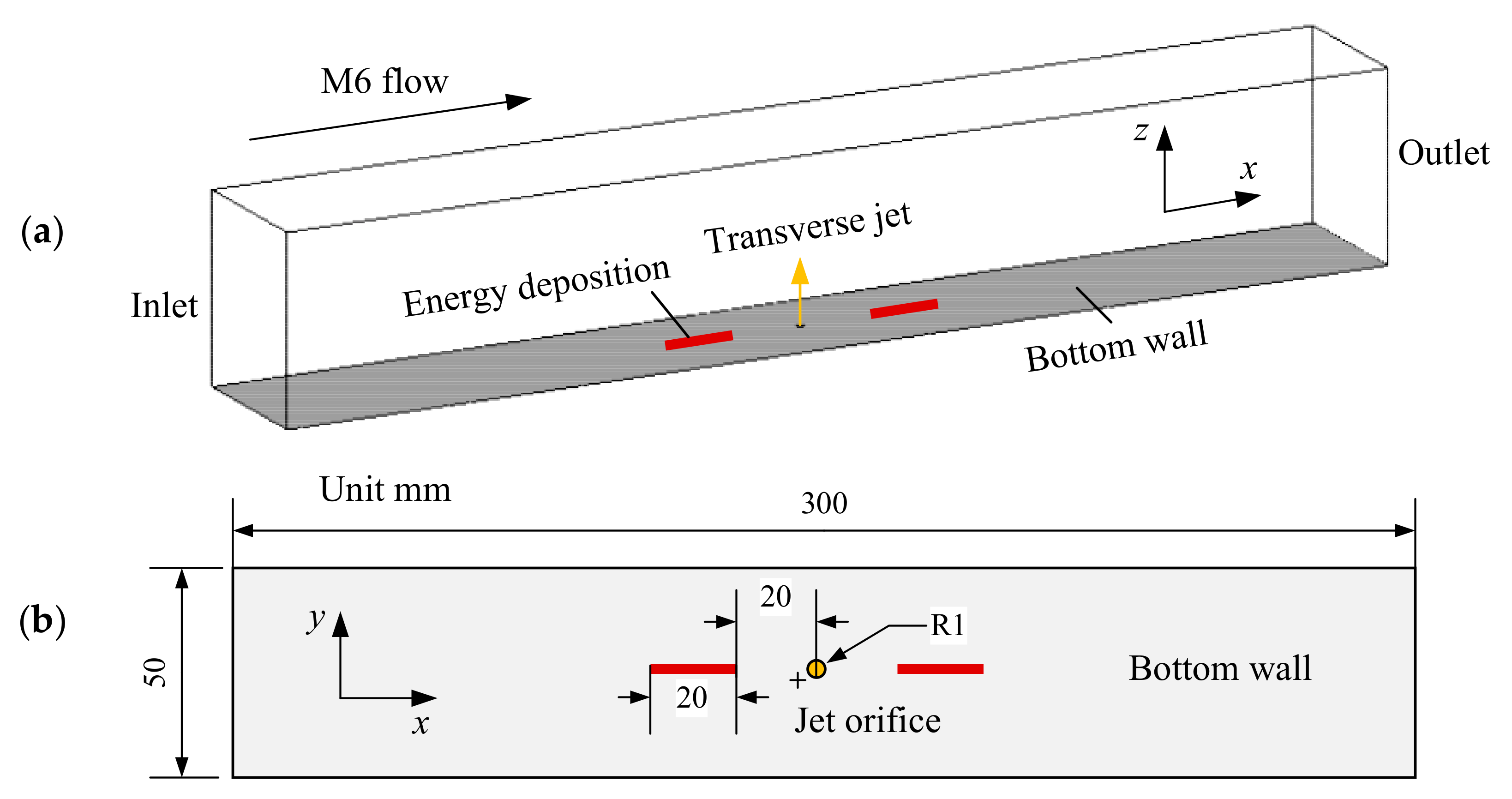
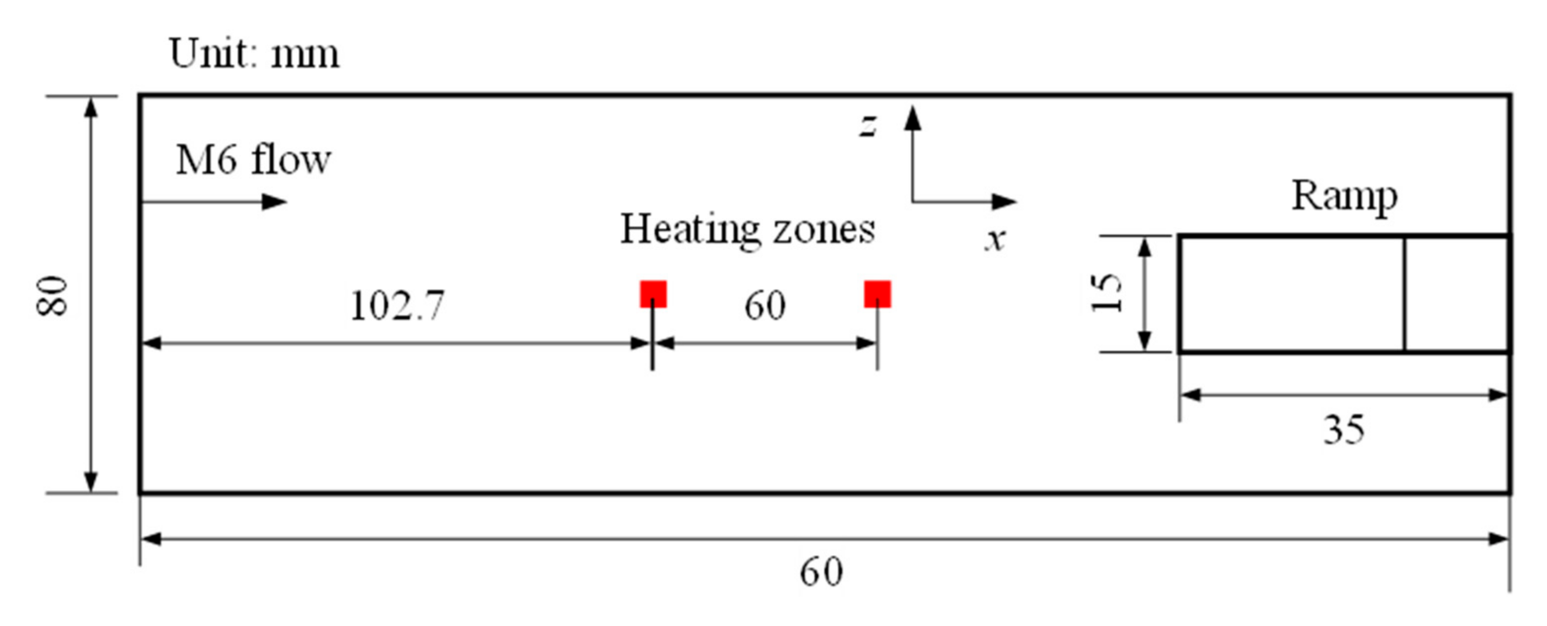
2.1. Physical Model

The utilized physical model is shown in Figure 1, with a total length of 300 mm, width of 50 mm, and height of 80 mm. The jet orifice is at x = 0 mm and has a diameter of 2 mm. The fuel medium is argon and is injected perpendicular to the jet orifice [20], and the supersonic incoming flow uses nitrogen as the medium. The numerical simulations are performed based on the condition where the momentum ratio of the jet transverse to the inflow is J = 8.68. Argon is often used as a tracer in experiments, and argon and nitrogen jets are selected to simulate real experimental environments.
The mixing of argon and nitrogen is controlled by the energy deposition as arranged along the flow direction, which are in the upstream (b) and downstream (c) positions of the jet orifice along the center line. These are denoted as Case b and Case c, while Case a is when there is no energy deposition. The energy deposition area is simplified into a cuboid heating area with a volume of 20 × 1 × 1 mm3, and the distance from the center of the orifice is Ld = 20 mm.
The computational grid of the model is shown in Figure 2, which adopts block-structured grids. The total number of the grids is approximately 3 million, with the wall grids intensified to ensure y+ = 1 × 10⁻⁶ m. The jet orifice is set as the mass flow inlet boundary condition, and the outlet is set as the pressure outlet boundary condition. The wall of the model is set as a no-slip adiabatic wall, and the other surfaces are set with far-field pressure conditions. The incoming flow is set as Ma = 6, and the static temperature is set as T = 36.5 K. The static pressure is set as p = 443 Pa, and the incoming flow is nitrogen. The argon flow rate at the orifice is 0.0002 kg/s, and the total temperature is Tj0 = 300 K. The dynamic viscosity coefficient μ is calculated through the Sutherland formula and is valued at 2.2 × 10⁻⁶ N.S/m2.

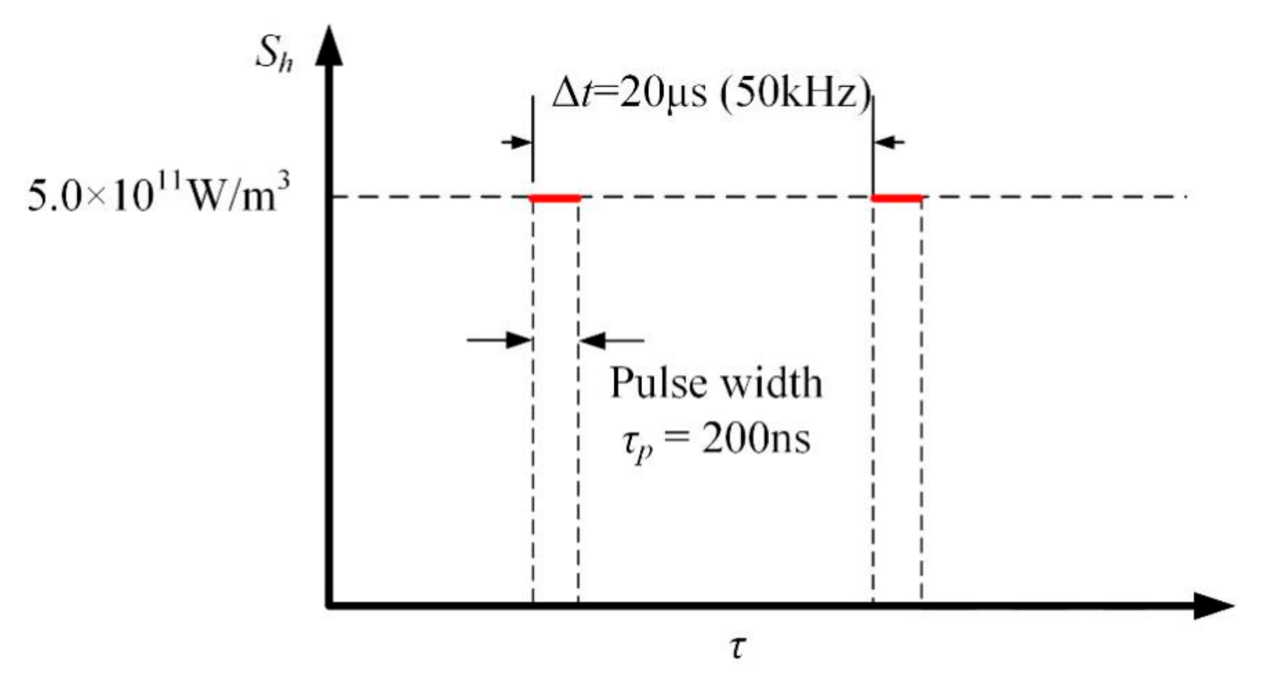
2.2. Numerical Method

The flow fields of the transverse jet model with and without energy depositions are simulated by solving the Reynolds-averaged N-S equations with an energy source term. The governing equation is the multi-component conservative N-S equation, which is expressed based on the Reynolds average in a Cartesian coordinate system as:
Q t + E x + F y + G z = E d x + F d y + G d z + S p
where Q is the conserved flux; E, F, and G are the opposite flux vectors in the x, y, and z directions, respectively; t is the time; Sp is the energy source term; and Ed, Fd, and Gd are diffusion flux vectors in the x, y, and z directions, respectively. The detailed equations of each variable are given as:
Q = [ ρ ρ u ρ v ρ w ρ e ρ Y i ] E = [ ρ u ρ u u + p ρ u v ρ u w u ( ρ e + p ) ρ u Y i ] F = [ ρ v ρ v u ρ v v + p ρ v w v ( ρ e + p ) ρ v Y i ] G = [ ρ w ρ w u ρ w v ρ w w + p w ( ρ e + p ) ρ w Y i ] H = [ S d , m S d , u S d , v S d , w S d , h w i ]
E d = [ 0 τ x x τ x y τ x z u τ x x + v τ x y + w τ x z q x ρ i D i m Y i / x ] F d = [ 0 τ y x τ y y τ y z u τ x y + v τ y y + w τ y z q y ρ i D i m Y i / y ] G d = [ 0 τ z x τ z y τ z z u τ z x + v τ z y + w τ z z q z ρ i D i m Y i / z ]
where i = 1,2… is the total number of components; ρ is the gas density; ρi is the density of component i; u, v, and w are the velocities along the x, y, and z axes, respectively; p is the pressure; e is the total energy; Yi is the mass fraction of component i; ωi is the mass generation rate of component i; Sd,m, Sd,u, Sd,v, Sd,ω, and Sd,h are the source terms of the gaseous phase interaction and chemical reaction, which are valued at 0 in the mixed flow field; and τij is the viscous stress component and its mathematical expression is given as:
{ τ x x = 2 3 μ ( · V ) + 2 μ u x τ y y = 2 3 μ ( · V ) + 2 μ u y τ z z = 2 3 μ ( · V ) + 2 μ u z
{ τ x y = τ y x = μ ( u y + v x ) τ y z = τ z y = μ ( w y + v z ) τ x z = τ z x = μ ( w x + u z )
The subscripts x, y, and z denote partial derivatives in the x, y, and z directions, respectively; and qx, qy, and qz are the energy fluxes along each coordinate axis caused by heat conduction and component diffusion.
{ q x = k T x ρ i = 1 N s D i m h i Y i x q y = k T y ρ i = 1 N s D i m h i Y i y q z = k T z ρ i = 1 N s D i m h i Y i z
where Dim is the mass diffusion coefficient of component i.
D i m = ( 1 X i ) i , j 1 X j D i j
where Xi is the mole fraction of the components. Under medium- and low-pressure conditions, the diffusion coefficient of the bicomponent mixed gas is given as:
D i = 1.883 × 10 2 T 3 · ( M i + M j ) / M i M j ρ σ 2 i j Ω D
where Mi and Mj are the molecular weights of gas components i and j, respectively; and σij is the characteristic length. The thermal energy of the mixed gas can be calculated as:
e = i = 1 N s Y i h i + 1 2 ( u 2 + v 2 + w 2 ) p ρ
The enthalpy of each component is given as:
h i = h f 0 + T t d T C p i d T
The turbulence model was selected as the SST k-ω model [20], which is a combination of the near-wall Wilcox 1988 k-ω model and the separation region k-ε model [21]. This model is considered because it better predicts the free shear flow characteristics and is not sensitive to initial values. Compared with the k-ω model, the turbulence model is less sensitive to the incoming flow turbulence. It also has a better performance when calculating flow fields with a backpressure gradient [21]. The transport equations of k and ω are as given elsewhere [22].
Under supersonic incoming flow conditions, the incoming flow Mach number is high, the momentum and ion effects caused by plasma discharge play a negligible role, and only the instantaneous heating effect produces a certain flow control effect. To facilitate the numerical calculations, the flow direction energy deposition is simplified into a single heat source model. The energy deposition process is equivalent to a Joule heating process and is known as a phenomenological method. Jin et al. [23] used power density as an energy source term in the energy equation to simulate the heating process. The power density was obtained by fitting an experimental power waveform. Their numerical results well match experimental schlieren images, which demonstrates the effectiveness when simulating the effects of energy deposition. A power density with a frequency of f = 50 kHz and a pulse width of 200 ns is used in our simulations, as shown in Figure 3. Equation (11) defines the power density Sh for the energy deposition [24], which is determined by the transient power q(τ), volume of the heating zones V(x, y, z), and energy conversion rate η0. The τ is the pulse width, which is the heating time of an energy deposition pulse. The power density of the heating zone within a single pulse is kept as Sh = 5.0 × 10¹¹ W/m3.
S p = { η Q 0 τ ( x , y , z ) = q ( τ ) V ( x , y , z ) ( x 1 < x < x 2 , y 1 < y < y 2 , z 1 < z < z 2 , 0 < τ < τ p ) 0 ( o t h e r s )

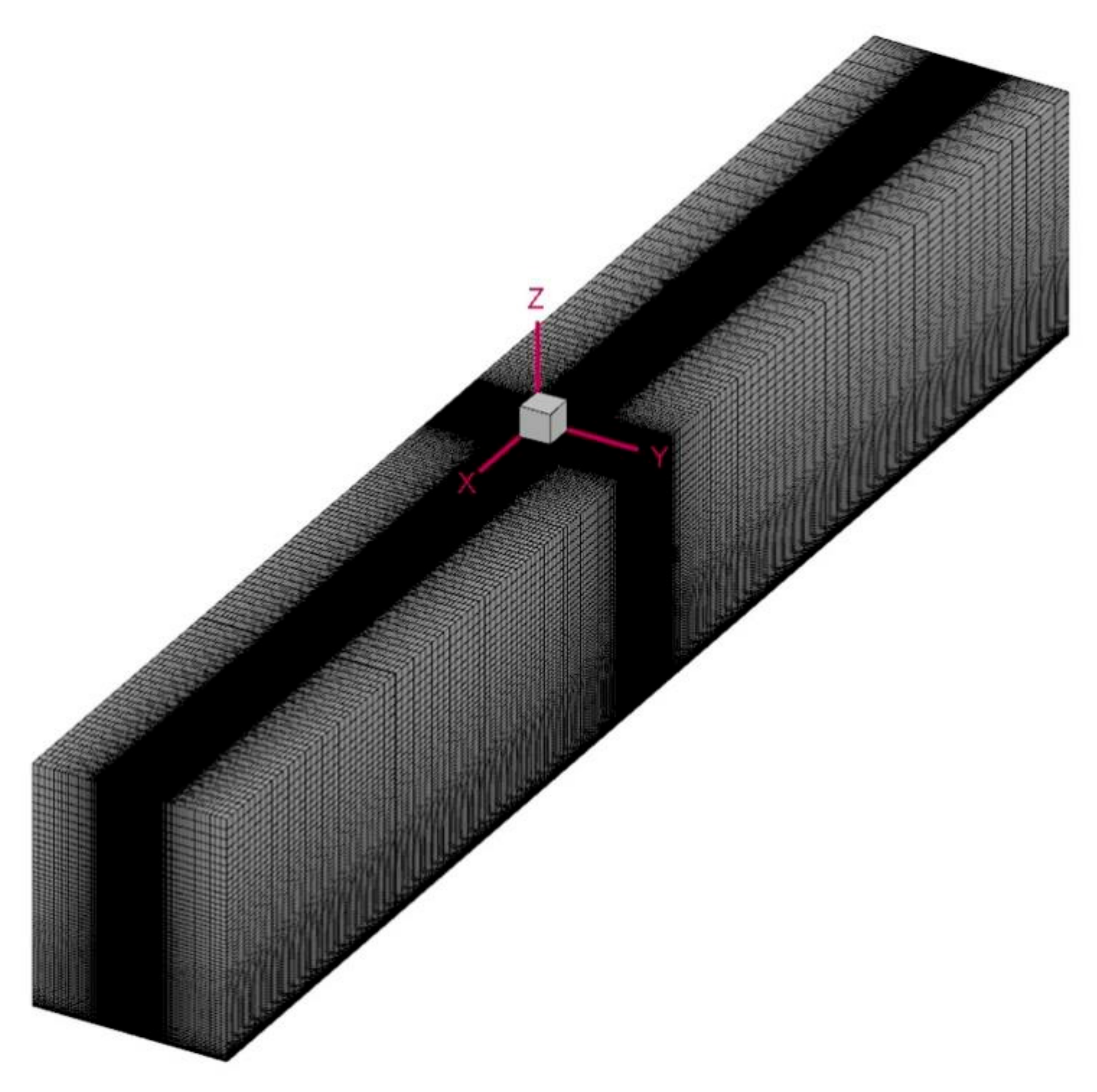
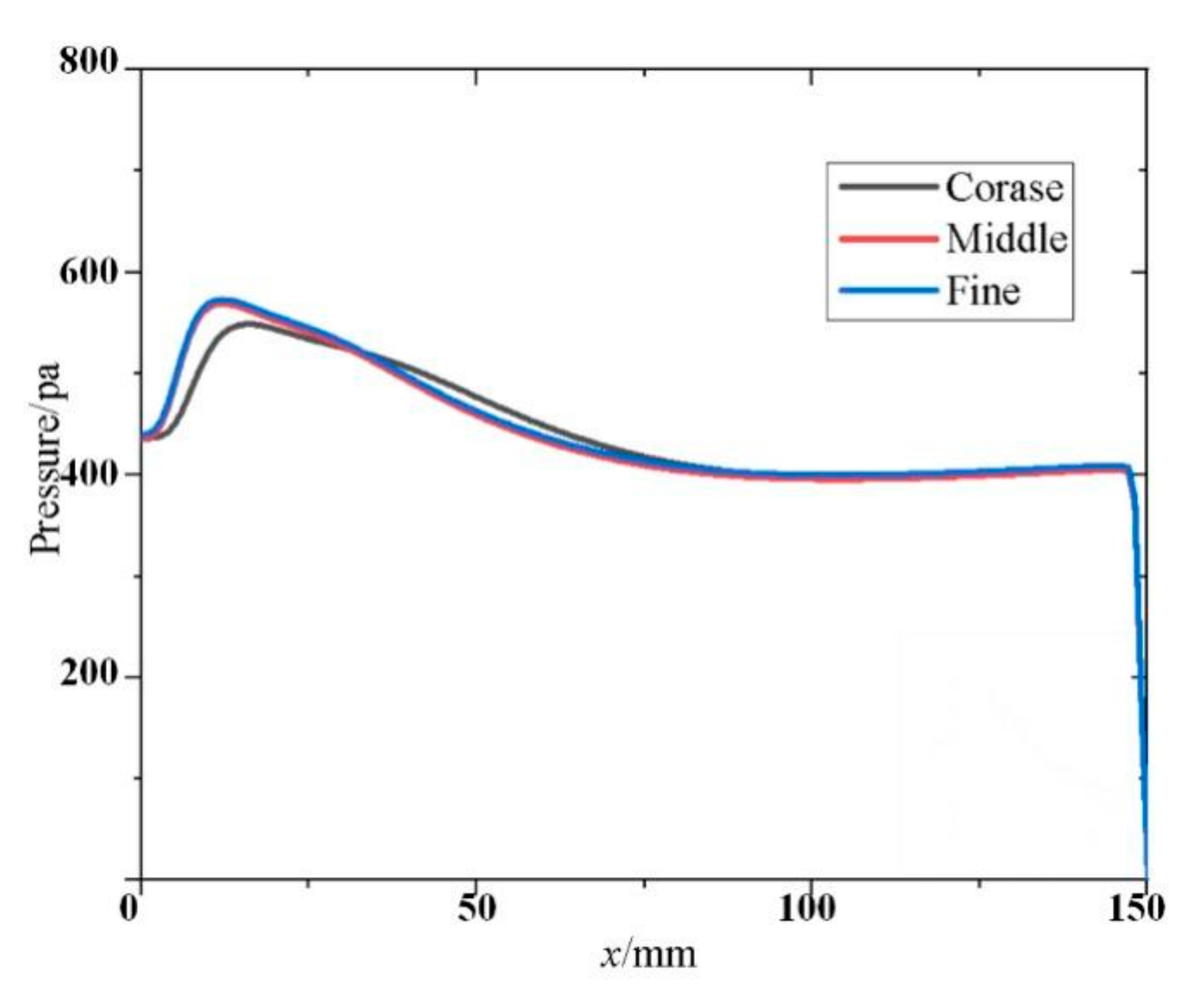
2.3. Grid Independence Study

In the finite element analysis, a finer mesh gives a greater precision for the solution. However, in practical designs and applications, the time cost of calculations increases greatly with the number of grids. Once the number of grids reaches a certain threshold, there is not a significant improvement in the calculation accuracy, making it necessary to verify the grid independence. Here, a coarse grid (1,800,000), middle grid (3,000,000), and fine grid (5,100,000) are selected to verify the grid independency. A comparison of the pressure values at z = 0.01 mm in the centerline of the model is shown in Figure 4. There is a large gap between the results of the coarse grid and the other two grids, while the curves of the other two are nearly coincident. Thus, the middle grid is selected based on the calculation accuracy and the number of grid calculations.

2.4. Numerical Validation

It is necessary to validate the reliability of our simulations from different aspects. The simulations of the heating effect from energy deposition on supersonic flow are verified based on the experimental schlieren images in Reference [25]. Their experiment was performed in a Ma = 6 wind tunnel, and a schematic diagram of the test model is shown in Figure 5. Our validation example and corresponding incoming traffic parameters as shown in Table 1 are the same as in the reference.
The density gradient diagram on the symmetry plane of the model is compared with the schlieren experimental results, as shown in Figure 6. The wave system structure, shear layer, and shock reattachment point positions of the schlieren image and density gradient are nearly the same, indicating that numerical simulations can accurately simulate the flow field state under plasma energy mass deposition.

3. Results and Discussion

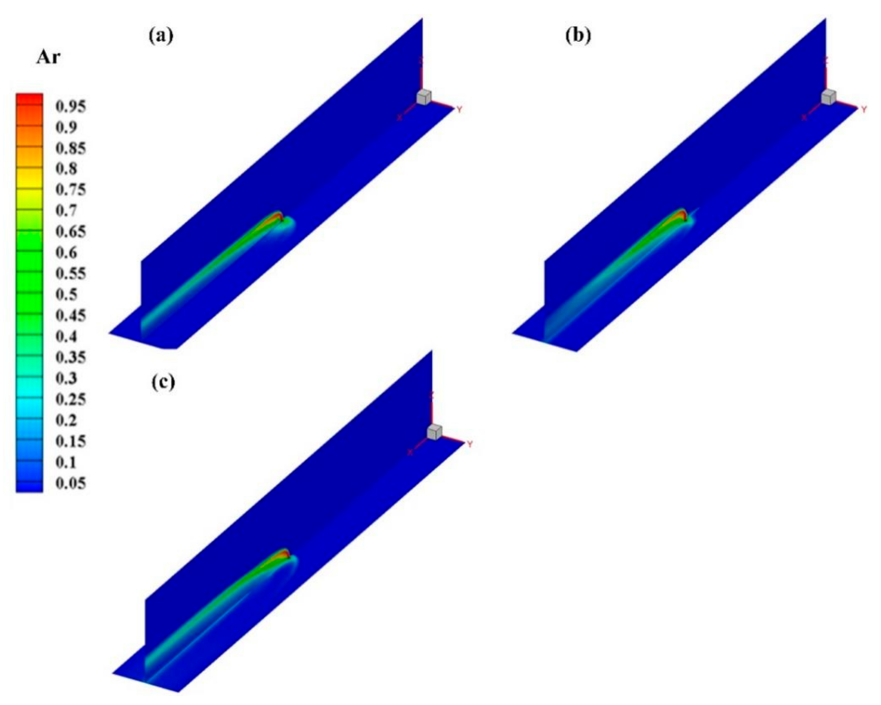
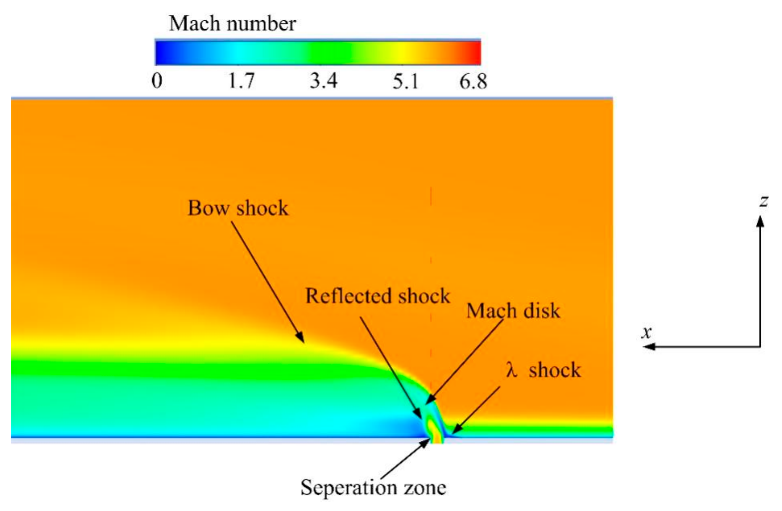
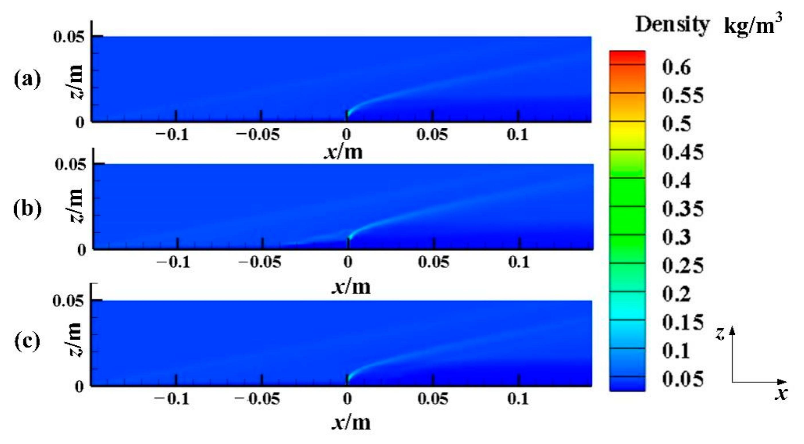
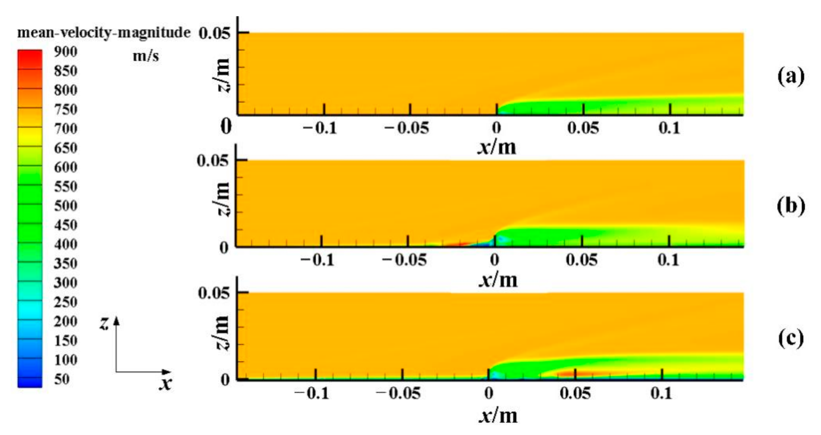
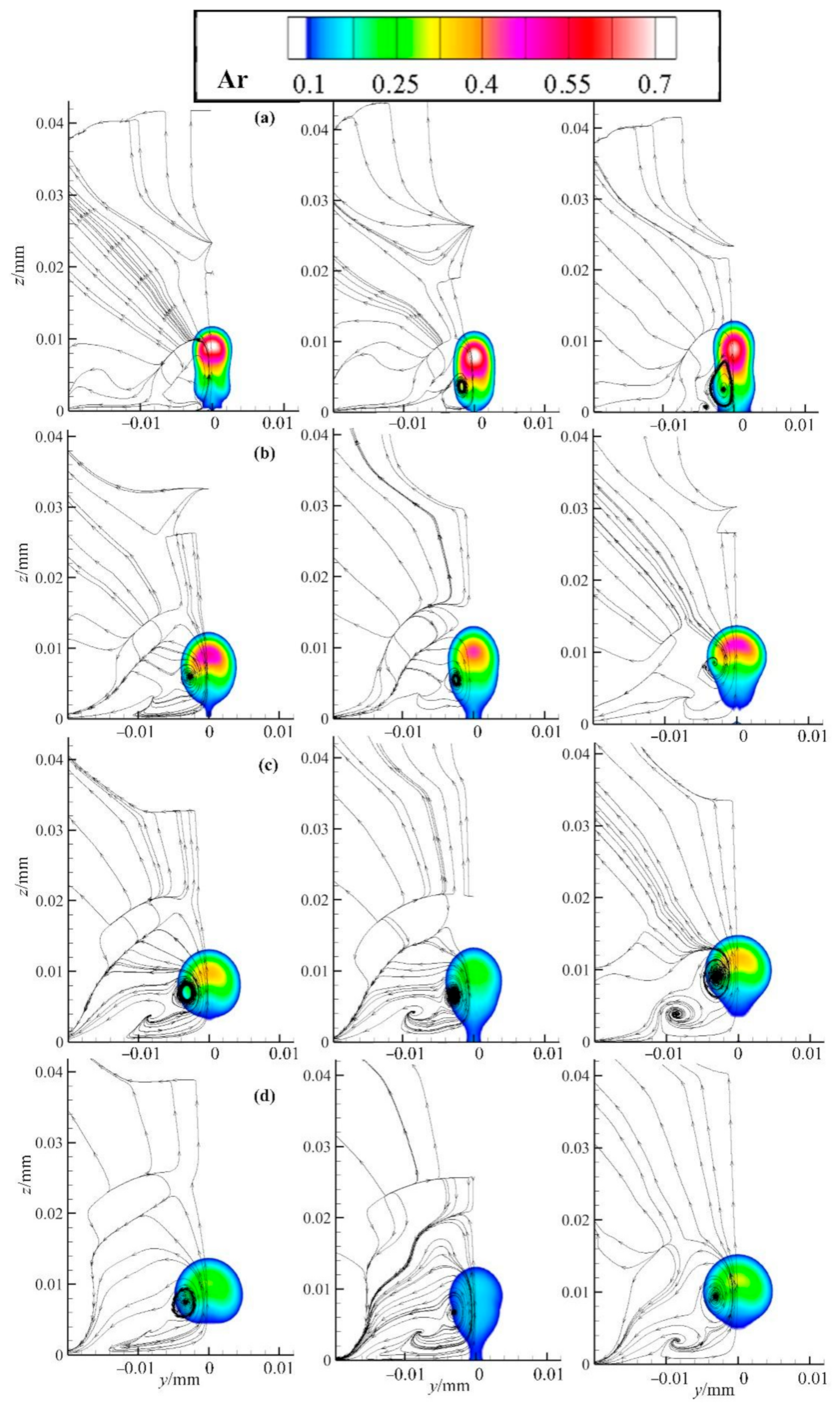
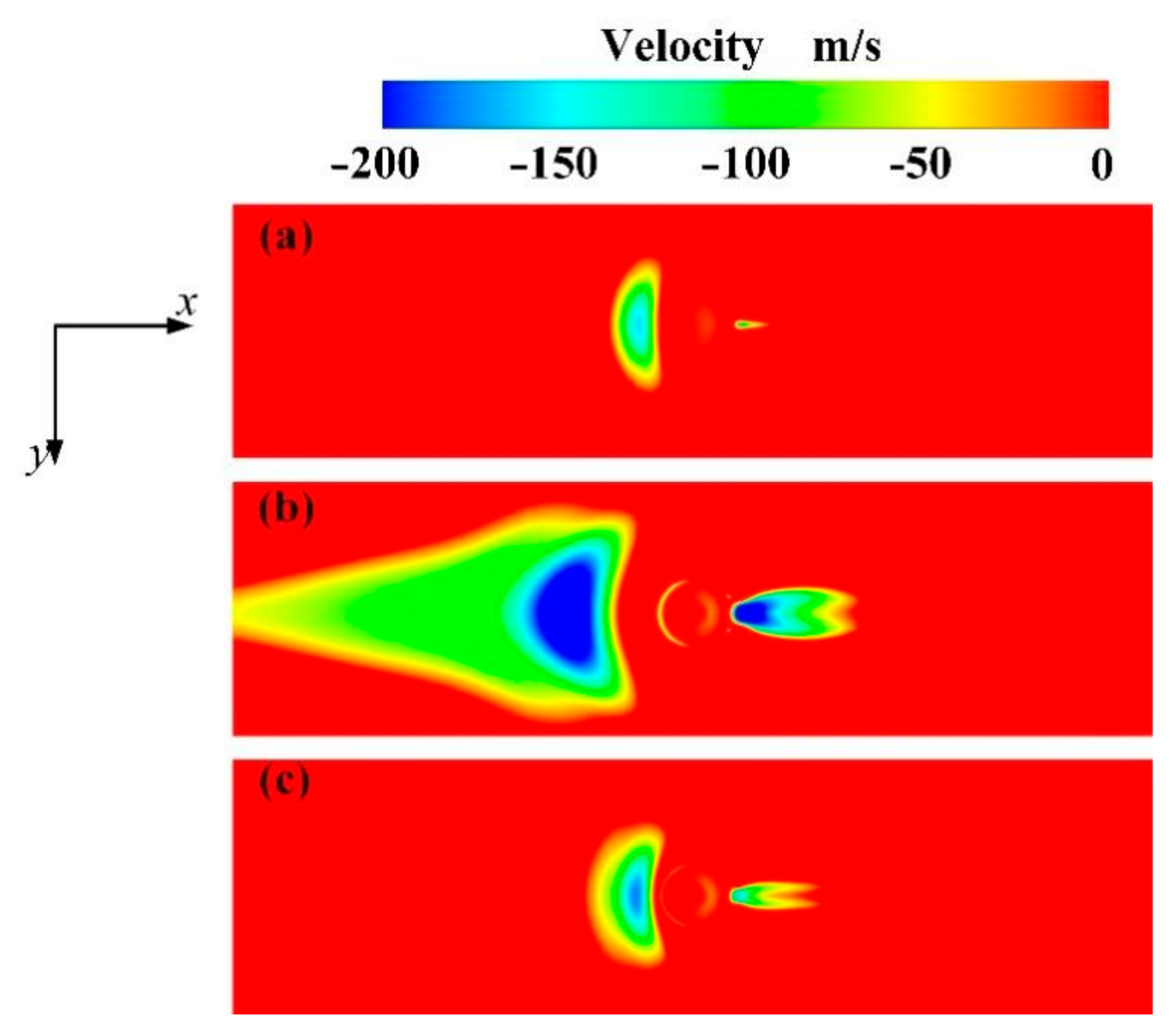
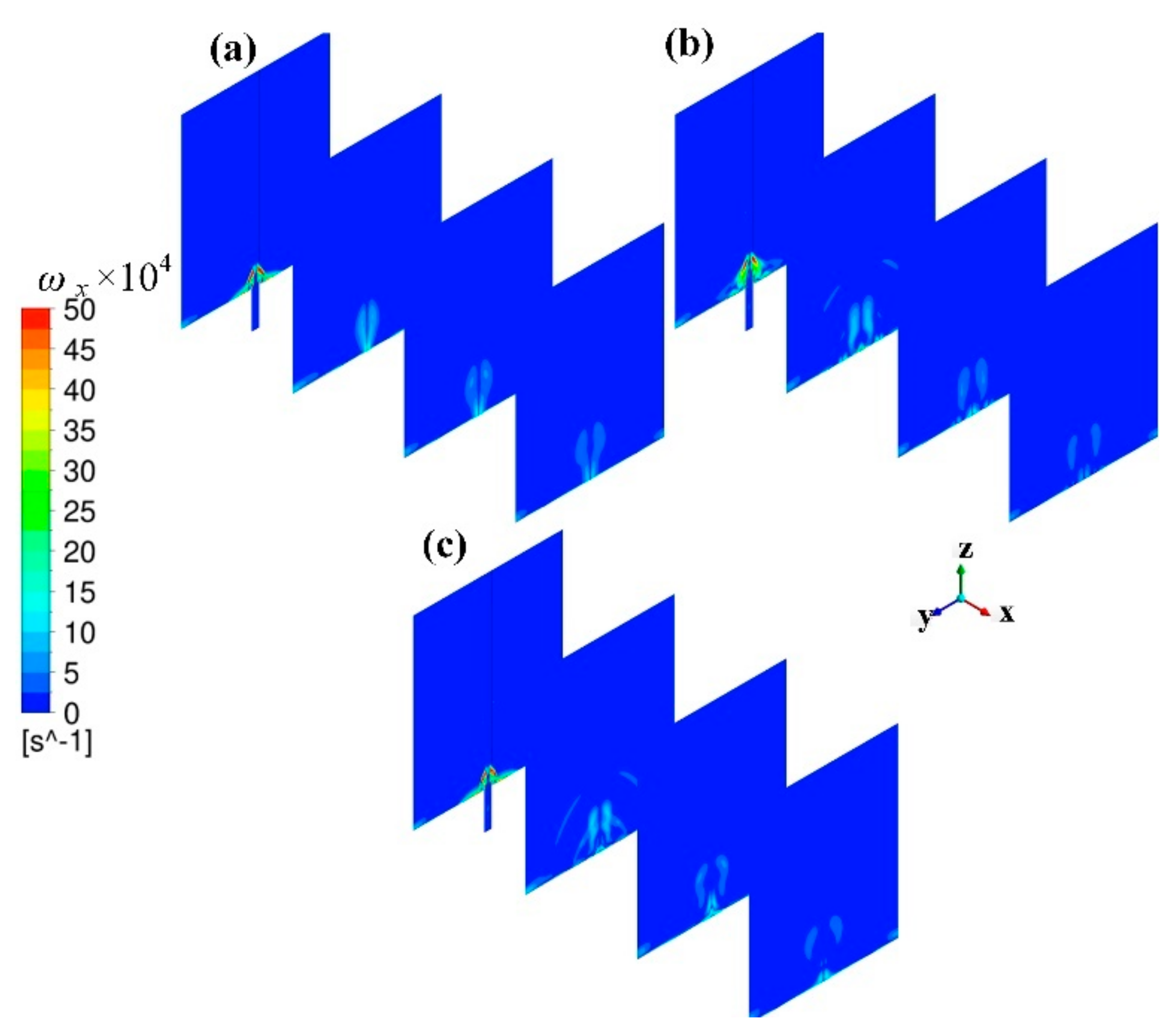
3.1. Argon Concentration Distribution and Flow Field Structure

The time-mean mass fraction contours of argon at the y = 0 and z = 0 sections under the three working conditions of Case a, Case b, and Case c are shown in Figure 7. Horseshoe vortex structures are formed around the jet orifices for all three cases. Under the action of supersonic free incoming flow, the jet column inclines downstream and its concentration decreases gradually with mixing. A larger x value gives a lower argon mass fraction. However, the argon in Case b is significantly thinner around the outlet than in the other two cases. At the outlet, the order of the penetration depth is Case c > Case b > Case a.
Figure 8 shows a schematic diagram of the transverse jet flow field for Case a. In the upstream region of the jet orifice, the adverse pressure gradient generated by the jet obstruction leads to flow separation in the incoming boundary layer. A separation shock wave, called the λ shock wave, is generated in the upstream region of the jet flow. A bow shock, Mach disk, reflected shock, and other structures are also observed.
Figure 9 and Figure 10 show density contours and the time-average velocity flow field for the three cases. In Figure 9, a bow shock is formed at the jet orifice by the transverse jet flow. This is due to the incoming flow being blocked by the jet, which results in a series of compression waves that converge in front of the jet orifice and form a bow shock. The density contours in Figure 9a,c are consistent, while the density contour in Figure 9b shows that the λ shock induced by the separation zone acts directly on the bow shock. Additionally, the angle of the bow shock is affected by the λ shock. The original angle is 24.7° in Case a, which then increases by 7.9° in Case b and 5.2° in Case c. The separation zone behind the jet orifice is also affected.
In Figure 10, the velocity of the jet is lower than that of argon in the flow field. The closer the jet is to the outlet, the greater its velocity. Figure 10a shows that the penetration depth of Case a gradually increases with x. Figure 10b shows that the velocity of the jet near the wall between x = −50–0 mm is relatively high, and the penetration depth between x = 0–50 mm is larger than that for the other two cases. However, as x increases, its penetration depth gradually decreases. Figure 10c shows that the jet in the velocity flow field diagram is “separated” into upper and lower jets due to the existence of the downstream energy deposition. The upper jet starts to lift under the thermal effect of energy deposition, which leads to an increased penetration depth in Case c. At x ≥ 100 mm, the penetration depth of Case c is the largest among the three cases.
Figure 11 shows the mass fraction contour diagram of the argon components and the corresponding streamlines for Case a, Case b, and Case c at the x = 30, 60, 90, and 120 mm planes under the flow field. Clipped regions with a mass fraction scope of YAr ≥ 0.1 are displayed. The argon jet evolves into typical vortex structures in supersonic flow, which facilitates fuel mixing. Figure 11 shows that in each case, a large-scale counter-rotating vortex pair (CVP) is formed due to the interactions between the mainstream and the jet, and most of the ethylene components are transported to this region. At the x = 30 mm section, the argon distributions for the three cases are nearly the same. Under the CVP, the jet plume develops downstream along the airflow and diffuses perpendicular to the wall surface. At the x = 60 mm section, the comparison of the three cases shows that the maximum argon concentration is the lowest in Case b and is nearly the same in Case c and Case a. The penetration depth of argon perpendicular to the wall in Case b and Case c significantly increases, and the high concentration zone for the three cases all decrease.
At the x = 90 mm section, the maximum argon concentration in Case a and Case c is still high, while both the maximum argon concentration and its high concentration area in Case b are smaller than in Case a and Case c. The order of the penetration depth for the three cases along the z direction is Case c > Case b > Case a. The three cases form two pairs of CVP structures in the same direction due to the interactions between the jet and mainstream. Meanwhile, the CVP scale of the latter two is larger than that for Case a. At the x = 120 mm section, the penetration depth of Case c is the largest. There is nearly no high-concentration area in Case b, and the streamwise vortex scale of the latter two is significantly larger than that of Case a. Therefore, the distribution of streamwise vortexes is related to the high-concentration region of argon, and the location and scale of the streamwise vortexes affect the diffusion degree of the components. The addition of energy deposition promotes the development of flow vortexes and expands their scale, which helps enhance fuel mixing. With an increased x value, the momentum component of the jet in the direction perpendicular to the wall continues to increase, giving a greater penetration depth in the vertical direction of the wall.

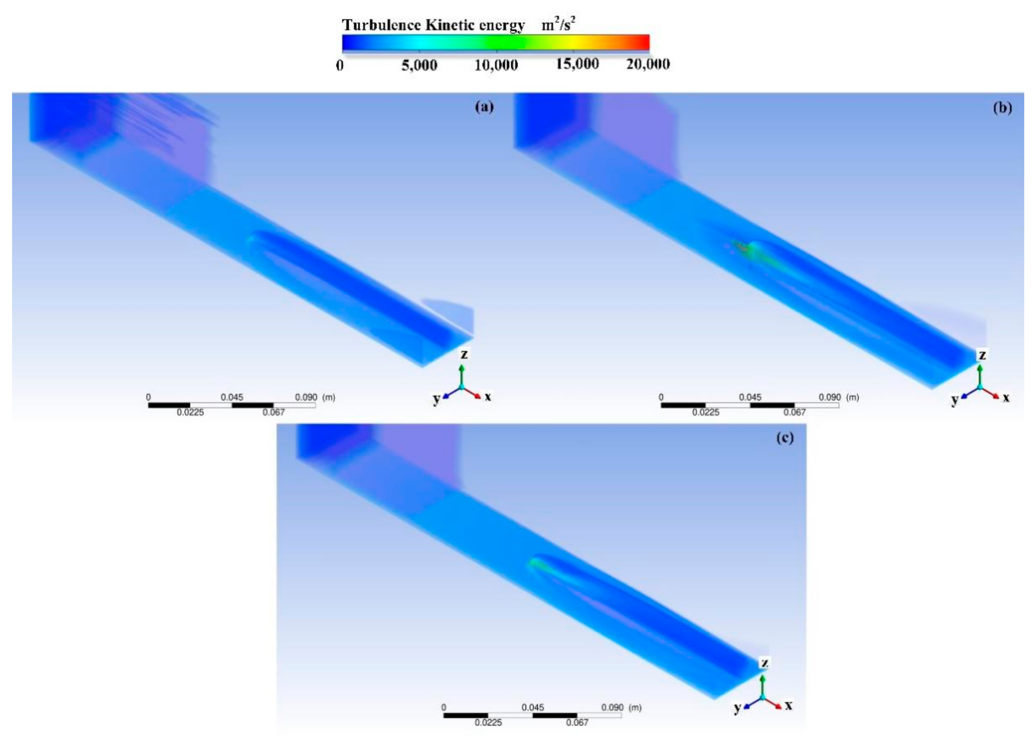
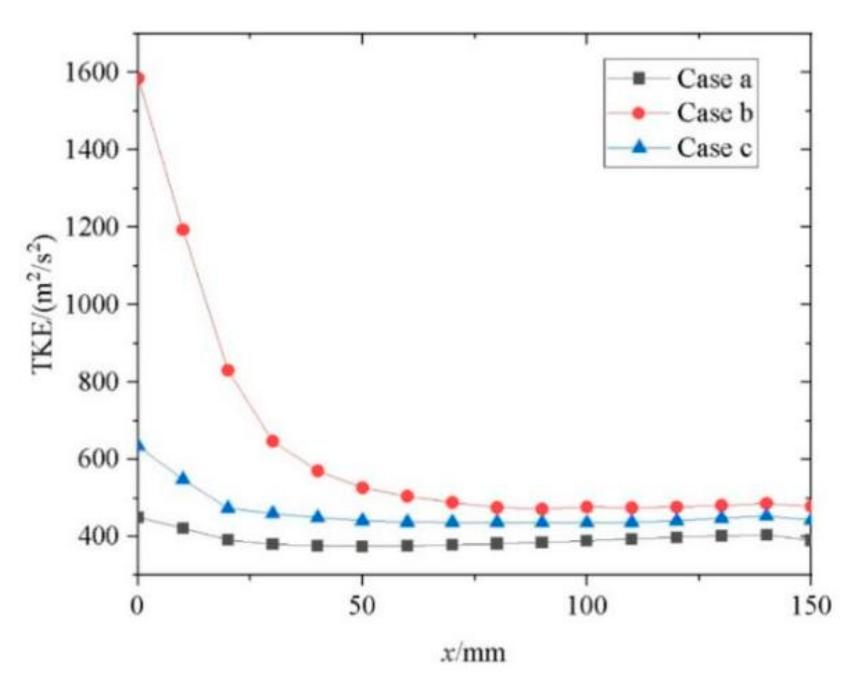
3.2. Turbulent Kinetic Energy Intensity
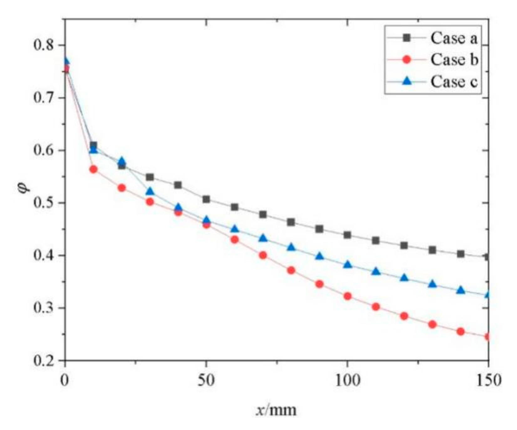
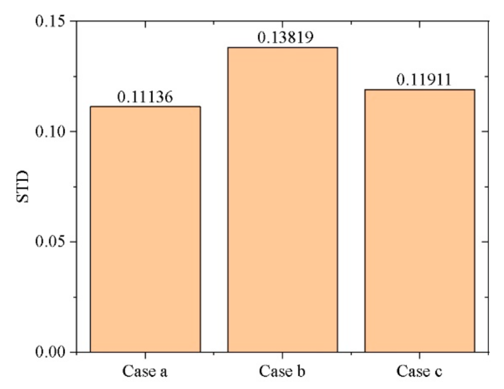
Turbulent kinetic energy is an important index that measures the turbulent pulsation in combustors. When the turbulent kinetic energy is high, it is conducive to mixing fuel and air. Figure 12 shows the turbulent kinetic energy volume rending diagram for the three cases. In comparison, the turbulent kinetic energy of the three cases is concentrated primarily in the vicinity of the jet orifice, which indicates that the turbulent pulsation is high in the jet vicinity, and the argon concentration changes more violently. The intensity of the turbulent kinetic energy decreases as it moves closer to the outlet, which means that changes in the argon concentration also decrease. Figure 12b shows that when the energy deposition is distributed upstream, the turbulent kinetic energy near the jet orifice increases significantly, which greatly improves the mixing efficiency of argon near the jet orifice. In Figure 12c, the turbulent kinetic energy in the upper part of the energy deposition slightly increases.
Figure 13 shows curves of the average turbulent kinetic energy for each section of the three cases. The trend of the three curves first drastically decreases and then gradually increases but by differing amounts. Among them, the change degree of Case b is the most drastic, followed by Case c. At the outlet, the average turbulent kinetic energy intensities for each section of the three curves are nearly the same.

3.3. Mixing Effect

The non-uniformity coefficient is introduced to quantitatively measure the mixing effect of argon in the nitrogen mainstream, which is shown as:
S = σ ϕ
where φ is the non-uniformity coefficient, σ is the variance of the concentration distribution along the cross-section, and Φ is the arithmetic square root of the concentration along the cross-section. Based on the definition of the non-uniformity coefficient, a smaller φ gives a better mixing of the two phases. When φ ≤ 0.05, the mixing is considered uniform, and the curves are shown in Figure 14, where φ decreases significantly along the x-axis. The φ values for Case a and Case c at x = 150 mm are nearly the same at 0.3975 and 0.3250, respectively, and that for Case b is 0.2460. Thus, the φ values of Case b and Case c are 61.5% and 32% lower than that of Case a, respectively.
The mean square deviation analysis is performed to analyze the fluctuation degree of φ in the three cases, where the mean square deviation is expressed as:
S = D ( m . ) = 1 N ( m i u m . u m i . )
where u m . and D ( m . ) are the mathematical expectation and variance of φ, respectively, m . is the non-uniformity coefficient, and a bar chart of the standard deviation is shown in Figure 15. The mean square deviation of φ is low when the energy deposition is distributed downstream and is valued at 0.11911. Thus, the mixing is more uniform when the energy deposition is downstream of the jet orifice.
Figure 14 shows there are some unsteady data points in Case b and Case c. From x = 20–30 mm, the rate of increase for φ in Case c is lower than the other two cases. This is because the energy deposition is located from x = 30–40 mm. This causes the flow above the energy deposition to spread in all directions and leads to a decreased rate of increase for φ. Before x = 60 mm in Case b, the rate of increase for φ is the greatest among the three cases. This is because before x = 60 mm there are several large-scale structures in the flow field, which benefits the mixing effect.
The curves of the maximum concentration value αmax for the section with changes in the dimensionless flow direction distance [26] effectively reflect the decrease rate of the maximum concentration of argon and the speed of fuel mixing, as shown in Figure 16. From x = 10–40 mm, the maximum concentration decay value for Case c is the greatest between the three cases. This is because the energy deposition in Case c causes some argon to flow back. The order of the maximum concentration at x = 150 mm is Case b < Case c < Case a, which are valued at 0.12333, 0.25813, and 0.29658, respectively. At the outlet, the maximum concentration of Case c is reduced by 15% compared with Case a, and that of Case b is reduced by 140%. Thus, the mixing effect is best when the energy deposition is distributed upstream of the jet orifice.

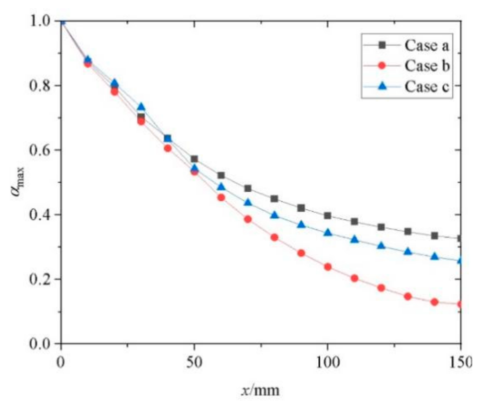
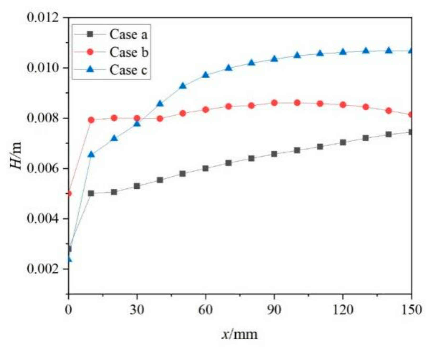
3.4. Penetration Depth

The penetration depth is defined as the mass-weighted average h+ of the fuel along the injection direction on the cross-section and is defined as [27]:
h + = ρ u ω A r H d A ρ u ω A r d A
where ω A r is the mass fraction of argon in the center of the grid cell; H is the coordinate value of the fuel injection direction based on the wall (coordinate of the wall where the jet orifice is located is set as 0); and ρ, u, and A are the density, velocity, and cross-sectional area of the center of the mesh, respectively. Equation (14) considers the mass-weighted average value of argon and comprehensively measures the spatial distribution of fuel. Therefore, this definition is chosen to evaluate the penetration depth for each considered case.
The penetration depth curves are shown in Figure 17. The penetration depth for Case b starts to decline slowly at x ≥ 90 mm. It is believed that shock induced by the upstream energy deposition acts on the bow shock and weakens it. Therefore, the penetration depth for Case b is larger at the downstream position near the jet orifice. At x ≥ 40 mm, the penetration depth for Case c is the largest between the three cases because the thermal effect of energy deposition lifts the jet flow. The penetration depth for Case c at x = 150 mm is about 0.010 m, for Case b is about 0.008 m, and for Case a is about 0.0074 m. Therefore, Case c has the best penetration effect. As a greater jet depth gives a better thermal protection performance, Case b has the best thermal protection performance.

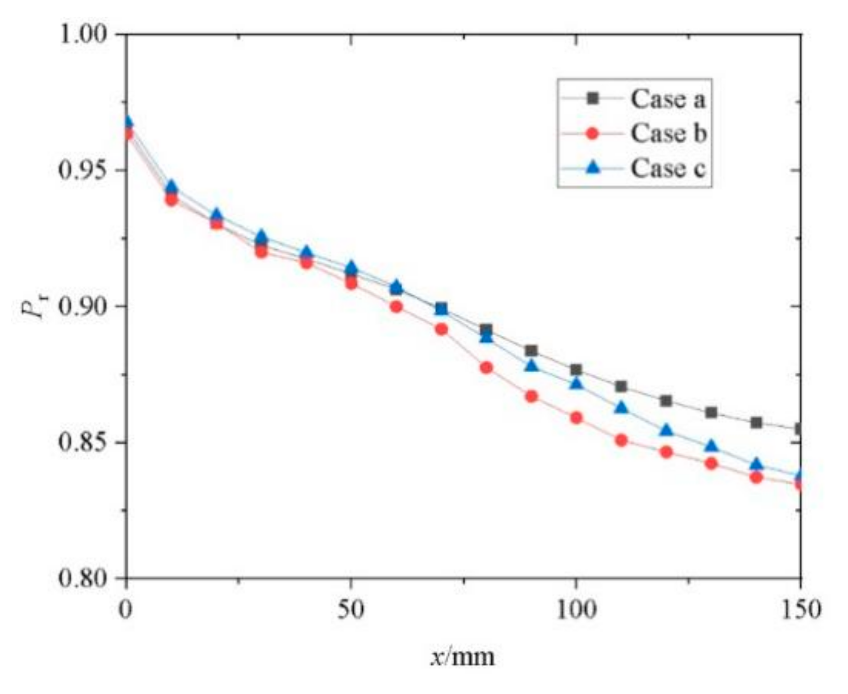
3.5. Total Pressure Recovery Coefficient

The total pressure recovery coefficient is among the more important indexes that measure the combustor performance. A larger total pressure recovery coefficient gives a stronger combustor outlet flow. The definition of the total pressure recovery coefficient is given as [28]:
p r = p t ρ u d A p ρ u d A
Figure 18 shows the total pressure recovery coefficient curves for Case a, Case b, and Case c. The total pressure recovery coefficient is greatest when there is no energy deposition, and it is smallest when the energy deposition is distributed upstream. However, there is little difference in the total pressure recovery coefficient between the three cases. Thus, the energy deposition increases the degree of turbulence, which intensifies the friction with the wall and increases the total pressure loss.

3.6. Influence Mechanism of Energy Deposition on the Transverse Jet

A schematic diagram of the reflux zone at z/D = 0.05 is illustrated in Figure 19 to explore the influence mechanism of the upstream and downstream energy deposition on the transverse jet. The energy deposition adds a significant area to the reflux flow and separation zone. In Case b, the upstream energy deposition causes the front separation zone to expand significantly, which induces a stronger λ shockwave and leads to a decreased bow shock intensity. The back separation zone also greatly expands. In Case c, the front and back separation zones expand slightly. The complex coupling between the separation zone and other flow structures affects the mixing efficiency of the flow field.
Figure 20 shows the intensity of the streamwise vortexes for Case a, Case b, and Case c. The energy deposition enhances mixing by enlarging the scale of the streamwise vortex structure. Additionally, the intensities of the streamwise vortexes for Case c above the energy deposition increase significantly, indicating the enhanced mixing of Case c is caused by thermal disturbances from the energy deposition that act directly on the jet plume. Figure 21 shows the intensity of the spanwise vortexes for Case a, Case b, and Case c. The intensities of the spanwise vortexes increase significantly in front of the bow shock for Case b relative to Case a and Case c, which indicates that the enhanced mixing for Case b is from the R-M instability at the bow shock wave interface.

4. Conclusions

The influence of the upstream and downstream high-frequency energy depositions on the mixing effect of transverse jets under hypersonic conditions is studied via numerical simulations and is compared to the case without energy deposition. The main conclusions are given as follows:
(1)
Energy deposition improves the fuel mixing efficiency to a certain extent, and its effect is significant when distributed upstream.
(2)
Energy deposition improves the penetration depth of the jet and slightly reduces the total pressure recovery coefficient. The penetration depth of the jet distributed downstream is larger than that upstream at the outlet. However, there is no relationship between the mixing effect and penetration depth.
The essence of the mixed enhancement mechanism of the energy deposition is that it promotes the development of streamwise vortex structures. The mixing enhancement mechanism from the energy deposition distributed upstream of the jet orifice is due to the R-M instability at the interface. This leads to an increased vorticity in the low-density flow and increases the turbulent kinetic energy. The mixing enhancement mechanism of the energy deposition distributed downstream of the jet orifice is that the increased turbulent kinetic energy near the jet orifice is from the strong turbulence expansion disturbance that forms, which acts directly on the jet plume. This stimulates plum instability and leads to an increased turbulent kinetic energy.

Author Contributions

Conceptualization, Z.C. and H.W.; methodology, F.G.; software, Z.C. and C.M.; validation, H.W.; formal analysis, H.W.; investigation, H.W.; resources, H.W.; data curation, Z.C.; writing—original draft preparation, Z.C.; writing—review and editing, Z.C.; visualization, T.Y.; supervision, H.W.; project administration, H.W.; funding acquisition, H.W. All authors have read and agreed to the published version of the manuscript.

Funding

This study is supported by the National Natural Science of China (Grant No. 12002363) and the National Key R&D Program of China (Grant No.2019YFA0405300).

Data Availability Statement

The data used to support the findings of this study are available from the corresponding author upon request.

Conflicts of Interest

The authors declare no conflict of interest.

References

  1. Li, L.Q.; Huang, W.; Yan, L.; Li, S.B.; Liao, L. Mixing improvement induced by the combination of a micro-ramp with an air porthole in the transverse gaseous injection flow field. Int. J. Heat Mass Transf. 2018, 124, 109–123. [Google Scholar] [CrossRef]
  2. Tu, Q.; Takahashi, H.; Segal, C. Effects of Pylon-Aided Fuel Injection on Mixing in a Supersonic Flowfield. In Proceedings of the 48th AIAA Aerospace Sciences Meeting Including the New Horizons Forum and Aerospace Exposition, Orlando, FL, USA, 4–7 January 2010. [Google Scholar]
  3. Huang, Z.W.; He, G.Q.; Qin, F.; Wei, X.G. Large eddy simulation of flame structure and combustion mode in a hydrogen fueled supersonic combustor. Int. J. Hydrogen Energy 2015, 40, 9815–9824. [Google Scholar] [CrossRef]
  4. Choubey, G.; Deuarajan, Y.; Huang, W.; Mehar, K.; Tiwari, M.; Pandey, K.M. Recent advances in cavity-based scramjet engine- a brief review. Int. J. Hydrogen Energy 2019, 44, 13895–13909. [Google Scholar] [CrossRef]
  5. Choubey, G.; Devarajan, Y.; Huang, W.; Shafee, A.; Pandey, K.M. Recent research progress on Transverse injection technique for Scramjet applications-a brief review. Int. J. Hydrogen Energy 2020, 45, 27806–27827. [Google Scholar] [CrossRef]
  6. Huang, W.; Wang, Z.G.; Wu, J.P.; Li, S.B. Numerical prediction on the interaction between the incident shock wave and the transverse slot injection in supersonic flows. Aerosp. Sci. Technol. 2013, 28, 91–99. [Google Scholar] [CrossRef]
  7. Huang, W.; Li, S.B.; Yan, L.; Wang, Z.G. Performance evaluation and parametric analysis on cantilevered ramp injector in supersonic flows. Acta Astronaut. 2013, 84, 141–152. [Google Scholar] [CrossRef]
  8. Mathur, T.; Gruber, M.; Jackson, K.; Donbar, J.; Donaldson, W. Supersonic Combustion Experiments with a Cavity-Based Fuel Injector. J. Propuls. Power 2001, 17, 10. [Google Scholar] [CrossRef]
  9. Ben-Yakar, A. Experimental Investigation of Mixing and Ignition of Transverse Jets in Supersonic Crossflows; Stanford University: Stanford, CA, USA, 2001. [Google Scholar]
  10. Leonov, S.; Isaenkov, Y.; Yarantsev, D.; Schneider, M. Fast Mixing by Pulse Discharge in High-Speed Flow. In Proceedings of the AIAA/AHI Space Planes & Hypersonic Systems & Technologies Conference, Canberra, Australia, 6–9 November 2013. [Google Scholar]
  11. Leonov, S.B.; Houpt, A.; Hedlund, B. Experimental Demonstration of Plasma-Based Flameholder in a Model Scramjet. In Proceedings of the 21st AIAA International Space Planes and Hypersonics Technologies Conference, Xiamen, China, 6–9 March 2017. [Google Scholar]
  12. Houpt, A.; Gordeyev, S.; Juliano, T.J.; Leonov, S.B. Optical Measurement of Transient Plasma Impact on Corner Separation in M=4.5 Airflow. In Proceedings of the Aiaa Aerospace Sciences Meeting, San Diego, CA, USA, 4–8 January 2016. [Google Scholar]
  13. Shi, J.; Hong, Y.; Bai, G.; Ke, L. Effect of Thermal Actuator on Vortex Characteristics in Supersonic Shear Layer. In Proceedings of the 47th AIAA Fluid Dynamics Conference, Denver, CO, USA, 5–9 June 2017. [Google Scholar]
  14. Ombrello, T.; Carter, C.; Mccall, J.; Schauer, F.; Naples, A.; Hoke, J.; Hsu, K.Y. Enhanced Mixing in Supersonic Flow Using a Pulse Detonator. J. Propuls. Power 2015, 31, 654–663. [Google Scholar] [CrossRef]
  15. Rogg, F.; Bricalli, M.; O’Byrne, S.; Pudsey, A.S.; Marzocca, P. Mixing Enhancement in a Hydrocarbon-Fuelled Scramjet Engine through Repeated Laser Sparks. In Proceedings of the 23rd AIAA International Space Planes and Hypersonic Systems and Technologies Conference, Montreal, QC, Canada, 10–12 March 2020. [Google Scholar]
  16. Zheltovodov, A.A.; Pimonov, E.A. The effect of localized pulse-periodic energy supply on supersonic mixing in channels. Tech. Phys. Lett. 2017, 43, 739–741. [Google Scholar] [CrossRef]
  17. Liu, F.; Yan, H.; Zheltovodov, A.A. Mixing Enhancement by Pulsed Energy Deposition in Jet/Shock Wave Interaction. AIAA J. 2021, 59, 1–11. [Google Scholar] [CrossRef]
  18. Tang, M.; Wu, Y.; Guo, S.; Sun, Z.; Luo, Z. Effect of the streamwise pulsed arc discharge array on shock wave/boundary layer interaction control. Phys. Fluids 2020, 32, 076104. [Google Scholar] [CrossRef]
  19. Zhou, S.; Nie, W.; Che, X. Numerical Investigation of Influence of Quasi-DC Discharge Plasma on Fuel Jet in Scramjet Combustor. IEEE Trans. Plasma Sci. 2015, 43, 896–905. [Google Scholar] [CrossRef]
  20. Huang, W.; Tan, J.G.; Liu, J.; Yan, L. Mixing augmentation induced by the interaction between the oblique shock wave and a sonic hydrogen jet in supersonic flows. Acta Astronaut. 2015, 117, 142–152. [Google Scholar] [CrossRef]
  21. Huang, W.; Liu, W.D.; Li, S.B.; Xia, Z.X.; Liu, J.; Wang, Z.G. Influences of the turbulence model and the slot width on the transverse slot injection flow field in supersonic flows. Acta Astronaut. 2012, 73, 1–9. [Google Scholar] [CrossRef]
  22. Segal, C. The Scramjet Engine: Processes and Characteristics; Cambridge University Press: Cambridge, UK, 2009. [Google Scholar]
  23. Di, J.; Wei, C.; Li, Y.; Li, F.; Min, J.; Quan, S.; Zhang, B. Characteristics of pulsed plasma synthetic jet and its control effect on supersonic flow. Chin. J. Aeronaut. 2015, 11, 66–76. [Google Scholar]
  24. Haack, S.; Taylor, T.; Emhoff, J.; Cybyk, B. Development of an Analytical Sparkjet Model. In Proceedings of the Flow Control Conference, Chicago, IL, USA, 28 June–1 July 2010. [Google Scholar]
  25. Wang, H.; Xie, F.; Li, J.; Yao, C.; Yang, Y. Study on control of hypersonic aerodynamic force by quasi-DC discharge plasma energy deposition. Acta Astronaut. 2021, 187, 325–334. [Google Scholar]
  26. Majumdar, S. Turbulence modeling for CFD, part 1. In Its CFD: Advances and Applications; SEE N95-19455 05-34; NAL: Bangalore, India, 1994; pp. 379–403. Available online: http://nal-ir.nal.res.in/id/eprint/3146 (accessed on 14 September 2022).
  27. Dehestani, P.; Fathi, A.; Daniali, H.M. Numerical study of the stand-off distance and liner thickness effect on the penetration depth efficiency of shaped charge process. Proc. Inst. Mech. Eng. Part C J. Mech. Eng. Sci. 2019, 233, 977–986. [Google Scholar] [CrossRef]
  28. Fedorova, N.N.; Fedorchenko, I.; Goldfeld, M.; Zakharova, Y. Mathematical modelling of supesonic flow over open cavity with mass supply. In Proceedings of the V European Conference on Computational Fluid Dynamics ECCOMAS CFD, Lisbon, Portugal, 14–17 June 2010. [Google Scholar]
Figure 1. Schematic diagram of the physical model for the numerical simulations: (a) Overhead view and (b) primary view.
Energies 15 08264 g001
Figure 2. Calculation area and mesh used in the simulations.
Energies 15 08264 g002
Figure 3. Diagram of arrayed pulsed energy deposition.
Energies 15 08264 g003
Figure 4. Curves comparing the accuracy with different numbers of grids.
Energies 15 08264 g004
Figure 5. Schematic diagram of the simplified model.
Energies 15 08264 g005
Figure 6. Comparison of the (a) experimental schlieren image and (b) the numerical density gradient contour in the case of PAPED.
Energies 15 08264 g006
Figure 7. Mass fraction contour diagrams of argon for (a) Case a, (b) Case b, and (c) Case c at z = 0 mm and y = 0 mm.
Energies 15 08264 g007
Figure 8. Diagram of the transverse jet flow field for Case a.
Energies 15 08264 g008
Figure 9. Density contour diagrams of (a) Case a, (b) Case b, and (c) Case c at y = 0 mm.
Energies 15 08264 g009
Figure 10. Time-average velocity flow field contour diagrams for (a) Case a, (b) Case b, and (c) Case c at y = 0 mm.
Energies 15 08264 g010
Figure 11. Mass fraction contours and streamline diagram of Case a, Case b, and Case c at x = (a) 30, (b) 60, (c) 90, and (d) 120 mm.
Energies 15 08264 g011
Figure 12. Turbulent kinetic energy volume rending diagrams for (a) Case a, (b) Case b, and (c) Case c.
Energies 15 08264 g012
Figure 13. Curves of the average turbulent kinetic energy in sections for Case a, Case b, and Case c.
Energies 15 08264 g013
Figure 14. Non-uniformity coefficients for Case a, Case b, and Case c along the x-axis.
Energies 15 08264 g014
Figure 15. STDs of Case a, Case b, and Case c.
Energies 15 08264 g015
Figure 16. Maximum concentration decay curves for Case a, Case b, and Case c.
Energies 15 08264 g016
Figure 17. Penetration depth curves for Case a, Case b, and Case c.
Energies 15 08264 g017
Figure 18. Total pressure recovery coefficient curves for Case a, Case b, and Case c.
Energies 15 08264 g018
Figure 19. Velocity contour diagram of the reflux zone for (a) Case a, (b) Case b, and (c) Case c at z/D = 0.05.
Energies 15 08264 g019
Figure 20. Intensity of the streamwise vortexes at x = 0, 30, 60, and 90 mm for (a) Case a, (b) Case b, and (c) Case c.
Energies 15 08264 g020
Figure 21. Intensity of the spanwise vortexes diagram at y = 0 mm for (a) Case a, (b) Case b, and (c) Case c.
Energies 15 08264 g021
Table 1. Parameters of the freestream used in the simulations.
Mach number M6
Total pressure p01.3 MPa
Total temperature T0300 K
Velocity u713 m/s
Static pressure p823.4 Pa
Static temperature T35.14 K
Publisher’s Note: MDPI stays neutral with regard to jurisdictional claims in published maps and institutional affiliations.

