Computational Investigation of Blade–Vortex Interaction of Coaxial Rotors for eVTOL Vehicles

Abstract

In the design of electric vertical takeoff and landing (eVTOL) vehicles, coaxial rotors have garnered significant attention due to their superior space usage and aerodynamic efficiency compared to standard rotors. However, it is challenging to study the flow field near the rotors due to the blade–vortex interface (BVI) and vortex–vortex contact between two rotors. Using sliding mesh technology and Reynolds-averaged Navier–Stokes (RANS) solvers, a numerical method was established to simulate the flow field of a coaxial rotor in hover, which was verified by experiments. Using this method, this paper analyzes the relationship between position and intensity of the tip vortex of the upper rotor, the axial velocity of induced flow and the load distribution on the blades at the azimuth when the BVI phenomenon occurs with a difference in rotational speed and rotor spacing. The results indicate that, when the BVI phenomenon appears, the blade-tip vortex of the top rotor rapidly dissipates, and the load distribution of the lower blade changes due to the induced flow of the vortex. When the rotational speed increases, the spanwise thrust coefficient of each rotor changes slightly. The vortex–vortex interaction becomes stronger, which leads to vortex pairing. When the distance between the rotors decreases, the BVI phenomenon occurs at an earlier azimuth and the location of the BVI moves towards the tip of the lower blade. The vortex–vortex interaction is also enhanced, which leads to vortex pairing and vortex merging.

1. Introduction

Electric vertical takeoff and landing vehicles, which are mainly used for urban short-distance passenger or cargo transportation and can effectively reduce traffic time and carbon emissions, have been rapidly developing in recent years. Due to their advantages over conventional rotorcraft, such as the simplicity of the drivetrain system, low acoustic noise, and safe operation in modern urban environments, multi-rotor electric vertical takeoff and landing (eVTOL) vehicles are generally more suitable than eVTOL with tiltwings and tiltrotors [1,2]. Currently, designers choose coaxial rotors over conventional rotors for eVTOL vehicles because the coaxial rotors not only have a high hover aerodynamic efficiency but also produce less noise during flight [3,4]. As fixed-wing aircraft, their flow field is relatively simple and its wake structure is stable [5,6]. However, the flow field of a coaxial rotor is often complex. The lower rotor is impacted directly under the effect of the upper rotor’s wake. Therefore, the wakes of the upper and lower rotors interact actively, which has a negative impact on the performance of coaxial rotors [7,8]. Due to the relative position of the two rotors, the blade–vortex interaction (BVI) phenomena may arise when the blade-tip vortex generated by the upper rotor interacts with the blade of the lower rotor, which may relate to the noise problem of coaxial rotors [3,9,10].

Researchers have carried out extensive studies on coaxial rotors. Harrington [11] presented several experiments and obtained the thrust performance of multiple full-scale coaxial rotors in hover. Landgrebe [12] investigated the performance and wake structure of a coaxial rotor. Ramasam [13] investigated the hover performance of a small-sized coaxial rotor, comparing single, tandem, and tilt-rotor designs. Leishman [14] developed the blade element momentum theory (BEMT), which is used to calculate the aerodynamic properties of coaxial rotor systems. Brown and Kim [15] created a vorticity transport model (VTM) and compared the hover and forward flight characteristics of a coaxial rotor with those of an equivalent single rotor. Tan and Sun [16] used the vortex particle method (VPM) combined with an unsteady panel technique to simulate the complex wake structure of a coaxial rotor in forward flight condition.

In recent years, computational fluid dynamics (CFD) technology has been widely used to investigate the flow field’s specifics in coaxial systems. Lakshminaryan and Baeder [17] investigated the aerodynamic performance and wake structure of the Harington coaxial rotor using the RANS solver in conjunction with the sliding mesh approach. Jeongwoo Ko [18] studied the wake dynamics of a coaxial rotor using a high-wake-resolution method combined with a truncated vortex tube model and a wave-number-extend finite-volume interpolation scheme to accurately capture flow field features such as the wake trajectory, blade–vortex interaction phenomenon, and wake instability phenomenon. Qi and Xu [19] created a numerical method based on the RANS equation and the moving overset mesh technique to simulate the aerodynamics of a Harrington coaxial rotor and found that the fluctuation feature of thrust can be explained by the “induction effect” and “overlap effect” caused by the interaction of wakes and bound vortexes of the coaxial rotor.

However, most of the work has focused on the study of unsteady aerodynamic characteristics of coaxial rotors. Although collision of circular vortex rings has been the subject of many systematic experimental and numerical investigations [20,21,22], the study of BVI on coaxial rotors is quite inadequate at present. The BVI phenomenon occurs as the vortex approaches the blade, influencing the distribution of aerodynamic load on the blade and causing partial load pulsation. The load pulsation will lead to serious vibration and noise from rotors, which is not favorable to the safety and comfort of flight. So, it is necessary to study the effects of some common parameters used in design on the BVI phenomena.

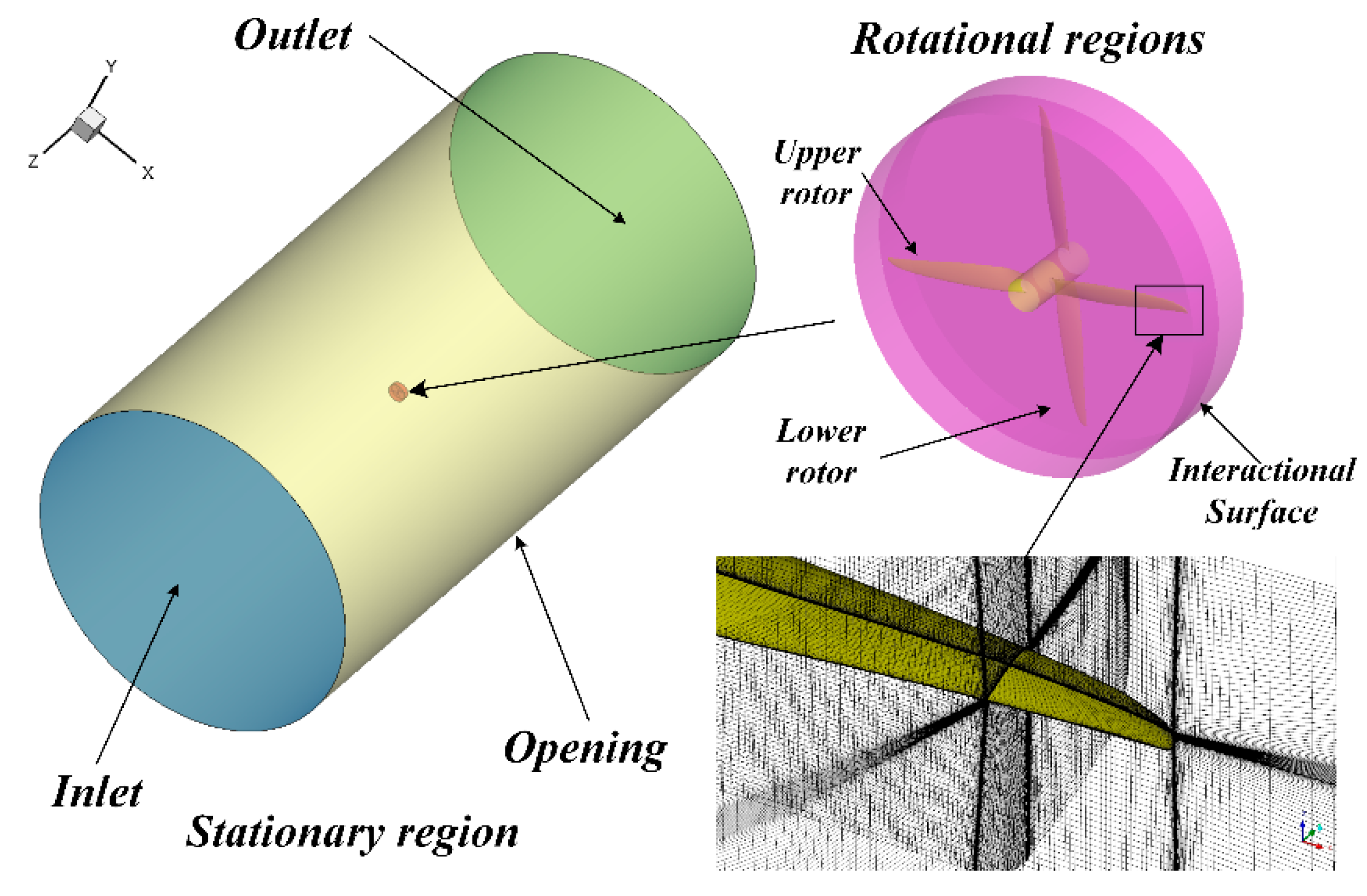
In this paper, the rotational motion of a coaxial rotor is simulated in different cases using a computational fluid dynamics (CFD) solver based on the unsteady Reynolds Average Navier–Stokes (uRANS) equation, which is verified by experiments. By analyzing the thrust coefficient distribution, position of the tip-vortex core and axial velocity of induced flow, the influence of azimuth gap, rotational speed and rotor spacing between two rotors on the BVI is analyzed and discussed.

2. Materials and Methods

2.1. Numerical Calculate Setup

Considering the unsteady characteristics of the coaxial rotor flow field, a conserved integral form of Navier–Stokes equations is established in the inertial coordinate system, which can be written as:

$$\frac{\partial }{\partial t}{\displaystyle \underset{V}{\iiint }W}dV+{\displaystyle \underset{S}{\iint }\left(F_c-F_V\right)\cdot ndS}=0$$

$$n={\left[\begin{array}{lll}{n}_x\hfill & n_y\hfill & n_z\hfill \end{array}\right]}^T$$

where S and V represent the surface area and volume of the contiguous volume, the vector W is a conserved variable. The vector F_c is for convective transport quantities and the vector F_V is for viscous fluxes, while n is the surface normal vector of the control element. All the variables can be written as follows:

$$W=\left[\begin{array}{c}\rho \\ \rho u\\ \rho v\\ \rho w\\ \rho E\end{array}\right].F=\left[\begin{array}{c}\rho V_{\mathrm{r}}\\ \rho u{V}_{\mathrm{r}}+n_{x}p\\ \rho v{V}_{\mathrm{r}}+n_{y}p\\ \rho w{V}_{\mathrm{r}}+n_{z}p\\ \rho H{V}_{\mathrm{r}}+V_{\mathrm{t}}p\end{array}\right]$$

$$F_v=\left[\begin{array}{c}0\\ n_x{\tau }_{xx}+n_y{\tau }_{xy}+n_z{\tau }_{xz}\\ n_x{\tau }_{yx}+n_y{\tau }_{yy}+n_z{\tau }_{yz}\\ n_x{\tau }_{zx}+n_y{\tau }_{zy}+n_z{\tau }_{zz}\\ n_x{\mathbf{\Phi }}_x+n_y{\mathbf{\Phi }}_y+n_z{\mathbf{\Phi }}_z\end{array}\right]$$

where ρ and p are the density and pressure of airflow, and E and H are the total energy and total enthalpy per unit mass, respectively, u, v, and w are the Cartesian velocity components, V_r is the relative velocity between blade and flow field, and V_t is the the relative velocity of mesh unit. τ_ij is related to viscous fluxes, while Φ_i is related to heat conduction.

The governing equations are spatially discretized using the finite volume method. [23] The spatial difference of the solver is calculated using high-resolution normalized variable diagram (NVD) approaches. To obtain the unsteady flow field of the coaxial system, temporal integration utilizes the dual time step approach and the multiple iteration display format in the pseudo time step. To regain high time accuracy in an unstable flow field, the subiteration of the pseudo time step is set to 10. Each time interval corresponds to 1 degree azimuth since the physical time step is set to 360 in one resolution of the rotor. Eddy viscosity is calculated using the two-equation k-ω SST turbulence model [24].

The sliding mesh technique is employed to represent the complicated rotational motion of two rotors. The grid is separated into stational and rotational regions. To increase mesh quality, each region’s mesh is created independently using a multiblock structured mesh generation technique. There are 45 million volume grid cells in all. The boundary layer consists of 25 grid layers, and the height of the first layer is 5 × 10⁻⁵ times the chord length c at 0.75 R of the blade. The mesh containing the rotor’s tip vortex is adjusted to capture the structure of vorticity with greater precision. The detail of the sliding mesh boundary condition is displayed in Figure 1.

2.2. Experimental Setup

To determine the aerodynamic performance of coaxial rotors, a modular, reconfigurable test bed comprised of two identical rotors in a coaxial rotor configuration was used. Figure 2 display a schematic representation of the entire test bed with rotors. The test bed was equipped with slide rails for continuous adjustment of the axial distance between the two rotors, allowing us to investigate the influence of rotor spacing on a coaxial rotor system. Each rotor was driven by the C14055 DC current through motor, whose rated power was 10 kW and maximum power was 20 kW. The rotational speed of the rotor on each side was controlled by the electronic speed control (ESC). In this experiment, a controller was programmed so that both motors rotate at the same rotational speed. The controller was designed so that the rotational speed discrepancy between a selected value and a measured value was input into an initial PID controller. The true rotational speed was acquired by an LSCI infrared temperature sensor, which measured the temperature on the blade’s surface and recorded the fluctuation of temperature when a blade passed though the detect region of the LSCI. Finally, the measured data were converted into current rotational speeds in the data acquisition system, whose average sampling rate was 10 Hz. The thrust of the rotor was measured by a TFC flame-typed force sensor, which had an accuracy of 0.1 N. The torque was measured by a TSD torque sensor with accuracy of 0.03 N∙m. The rotor model and its parameters are shown in Figure 3. Each rotor consisted of two blades and had a radius of R of 0.8 m, a hub diameter of 0.06 m, and a root cutout of 0.088 R. In the experiment, the performance of each rotor in different cases was measured by adjusting the rotating speed when the rotor spacing h/R was maintained as constant where h is the axial distance between two rotors.

2.3. Methodology Validation

We conducted a series of experiments in single and coaxial rotor configurations, and the coaxial experiment consisted of two two-blade rotors arranged to form a coaxial system. The radius of each rotor was 0.8 m at a spacing of h/R = 0.438 between the two rotors. Figure 4 shows the thrust and torque of each rotor at different rotational speeds. Comparing the data from the experiment, the thrust of each rotor was accurately predicted by numerical calculation with a maximum error of less than 4%. Compared with the results of the experiment, the maximum error of torque of the upper rotor by numerical calculation was less than 3%. However, the torque of the lower rotor obtained by calculation was generally higher than that of the experiment, and its maximum error almost reached 8%. The reason for the error may be the interpolation of the message exchanged through the interactional surface. The CFD solver used in this paper is able to accurately analyze the aerodynamic coefficients of a coaxial rotor system.

3. Results and Discussion

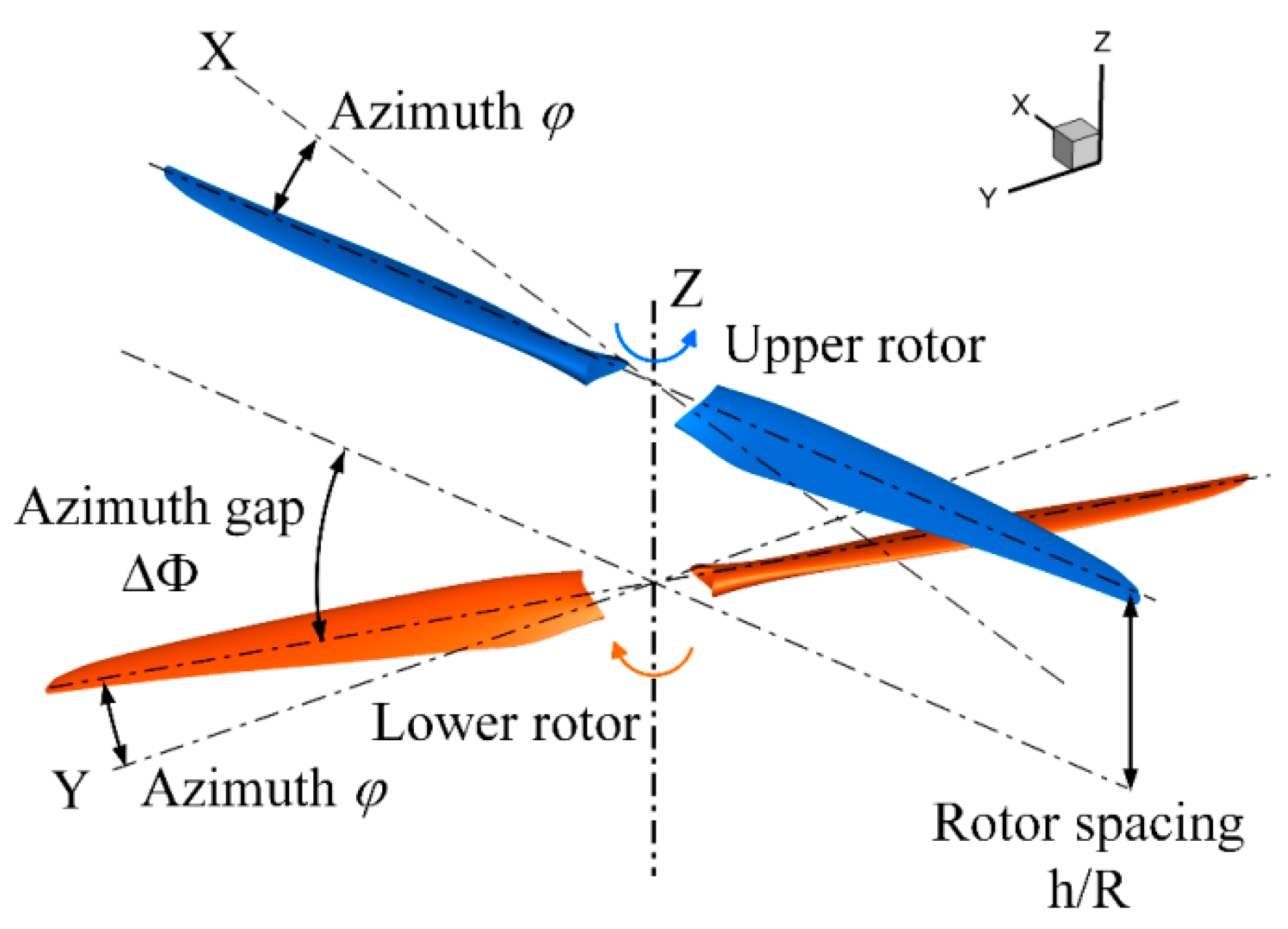
When viewed from above, in this research, each rotor in the coaxial rotor system had the same collective pitch, blade profile, and rotational speed but the upper rotor rotated anticlockwise and the lower rotor rotated clockwise. The origin of the global coordinate system was set at the hub center of the upper rotor. The z-axis coincided with the rotor shaft and headed up. The azimuth angles of the upper and lower rotors were measured in their respective directions of rotation. The pitch axes of upper blades were parallel to the x-axis at 0 degrees azimuth, and the pitch axes of lower blades were parallel to the y-axis. Figure 5 is a sketch map of the coaxial system’s blade locations.

3.1. Effect of Azimuth Gap

Blade–vortex interaction (BVI) appears when the tip vortex of the upper rotor is close to the blade of the lower rotor. In this section, several examples are discussed to describe the entire process in which the blades of the lower rotor pass through the wake of the upper rotor to research the effect of azimuth gap on the BVI. In this section, the rotor spacing between two rotors is maintained as h/R = 0.438 and the tip-Mach number is 0.517.

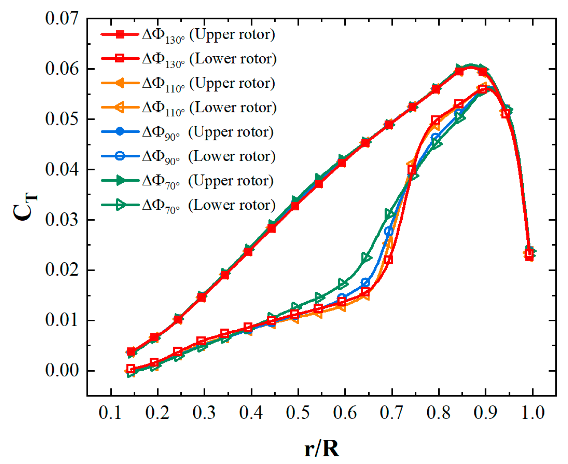
Figure 6 displays the variation in the spanwise distribution of thrust coefficient for each rotor at different azimuths. The local thrust coefficient can be calculated as follows:

$$C_T=\frac{dT}{\rho n^2{D}^4}\cdot \frac{R}{dr}$$

(1)

where ρ is the density of flow, n is the rotational speed, D is the diameter of rotor, R is the radius of rotor, dT is the thrust of local blade element, dr is the span of local blade element.

Figure 6 shows that, under the upper rotor’s induced flow, the thrust coefficient of the lower rotor was often smaller than that of the upper rotor, because the actual attack angle of the lower blade was affected by induced flow. Similarly, when the BVI phenomenon occurred at a 90-degree azimuth gap, the flow induced by the tip vortex of the upper rotors influenced the flow field near the lower blade by increasing the axial velocity on one side of the vortex and decreasing it on the other, thus altering the partial attack angle of the blade and causing a partial lift offset. Therefore, within the region of 0.6 R to 0.9 R, the C_T spanwise distribution curve shows an S-shaped fluctuation. Away from the interference of the BVI, the C_T distribution of the upper rotor was similar at different azimuth gaps. At an azimuth gap of 90 degrees to 130 degrees, the C_T distribution of the lower blade changed a little, which indicates that the BVI was still strong. At an azimuth gap of 70 degrees, the S-shaped fluctuation of the curve went down, which indicates that the BVI gradually diminishes because the tip vortex of the upper rotor moves away from the lower blade.

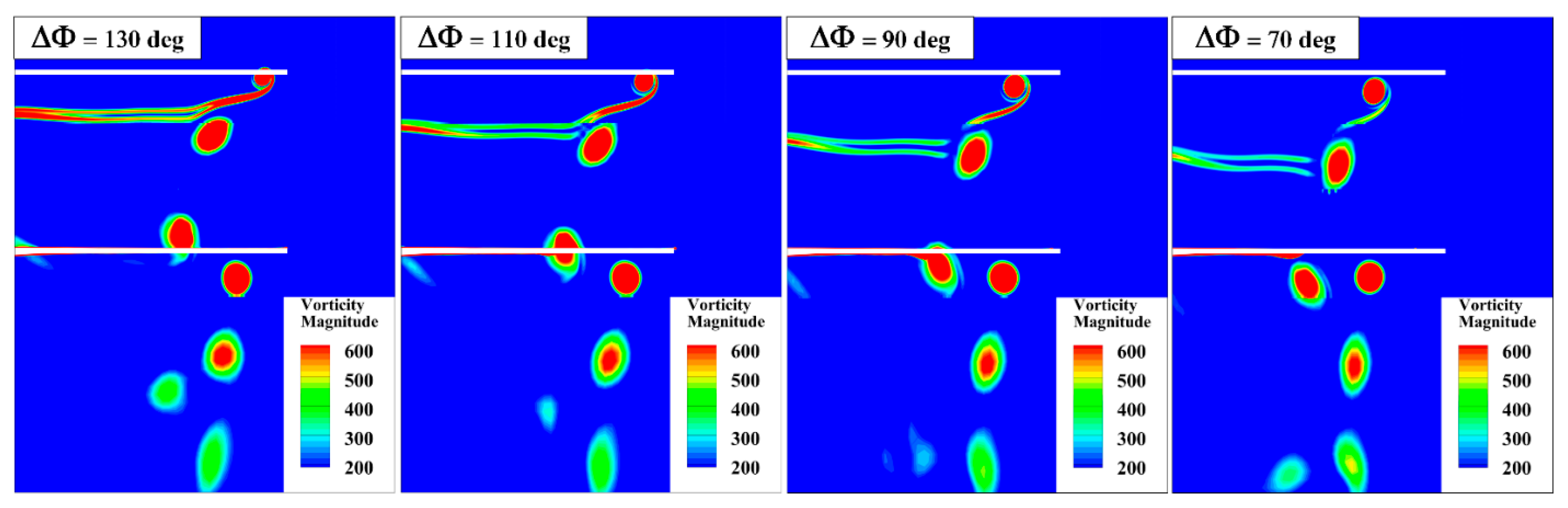
Figure 7 displays the vorticity magnitude contours at the vertical slice where the lower blades were located. When the azimuth gap was 130 degrees, the wake of the upper rotor passed over the lower blade. The wake structure of the upper rotor remained stable without being disturbed directly by the lower blade. When the azimuth gap was between 90 degrees and 110 degrees, the wake of the upper rotor directly passed across the lower blade. Disturbed by the surface and bound vortex of the lower rotor, the tip vortex of the upper rotor broke down and dissipated quickly. When the azimuth gap was 70 degrees, the tip vortex passed underneath the lower blade and the upper rotor’s wake recovered stability because of the decrease of BVI. Moreover, when the tip vortex passed through the lower blade, on the left hand of the vortex, the local Kutta condition [25] of the lower blade was disturbed by the induced flow of the vortex so that the wake of the lower blade moved downward.

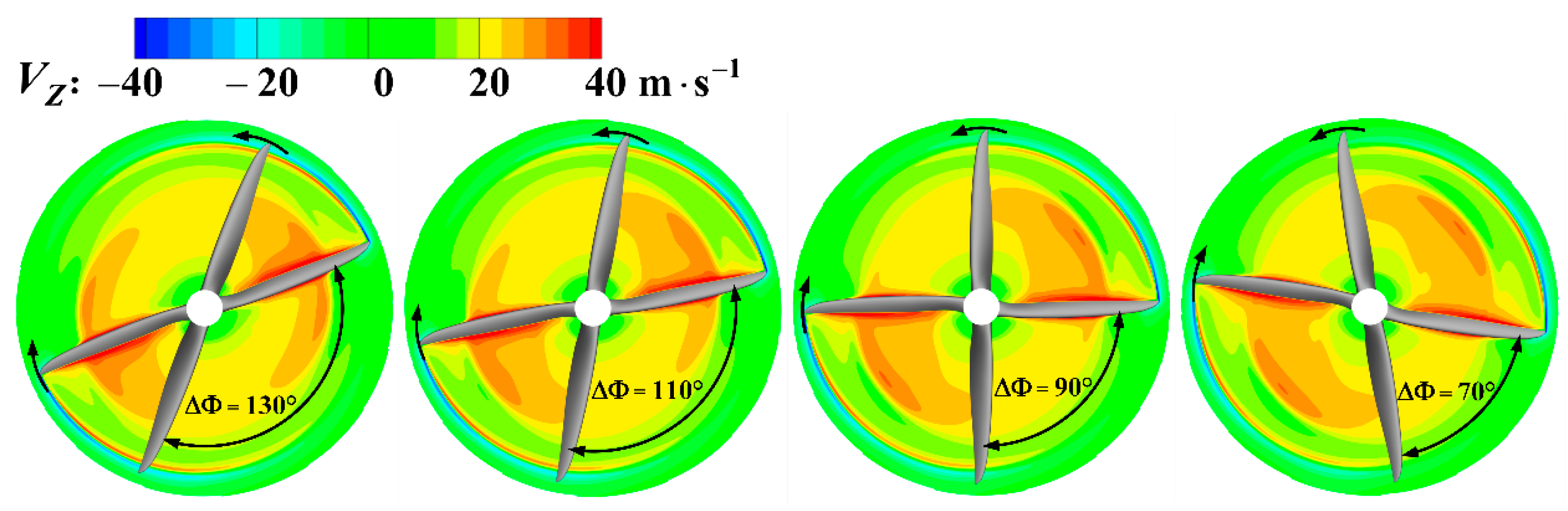
Figure 8 displays the axial induced velocity distribution of the horizontal slice where the lower rotor is located. When the BVI phenomenon occurred at an azimuth of 90 degrees to 130 degrees, the area where the tip vortex passed across the horizontal section was close to the lower blade, and the partial axial induced velocity increased, which verifies the reason for the partial lift offset on the lower blade. As the azimuth gaps between two rotors decreased, the upper blade and its tip vortex moved to the latter azimuth. However, for lower blade, due to the opposite rotational direction, the tip vortex actually went through the horizontal section at an earlier azimuth. With addition of the movement of the lower rotor, the region affected by the tip vortex was far away from the lower blade. This means that the vortex of the upper rotor had little interference with the lower blade, so that the BVI phenomenon decreased.

3.2. Effect of Rotational Speed

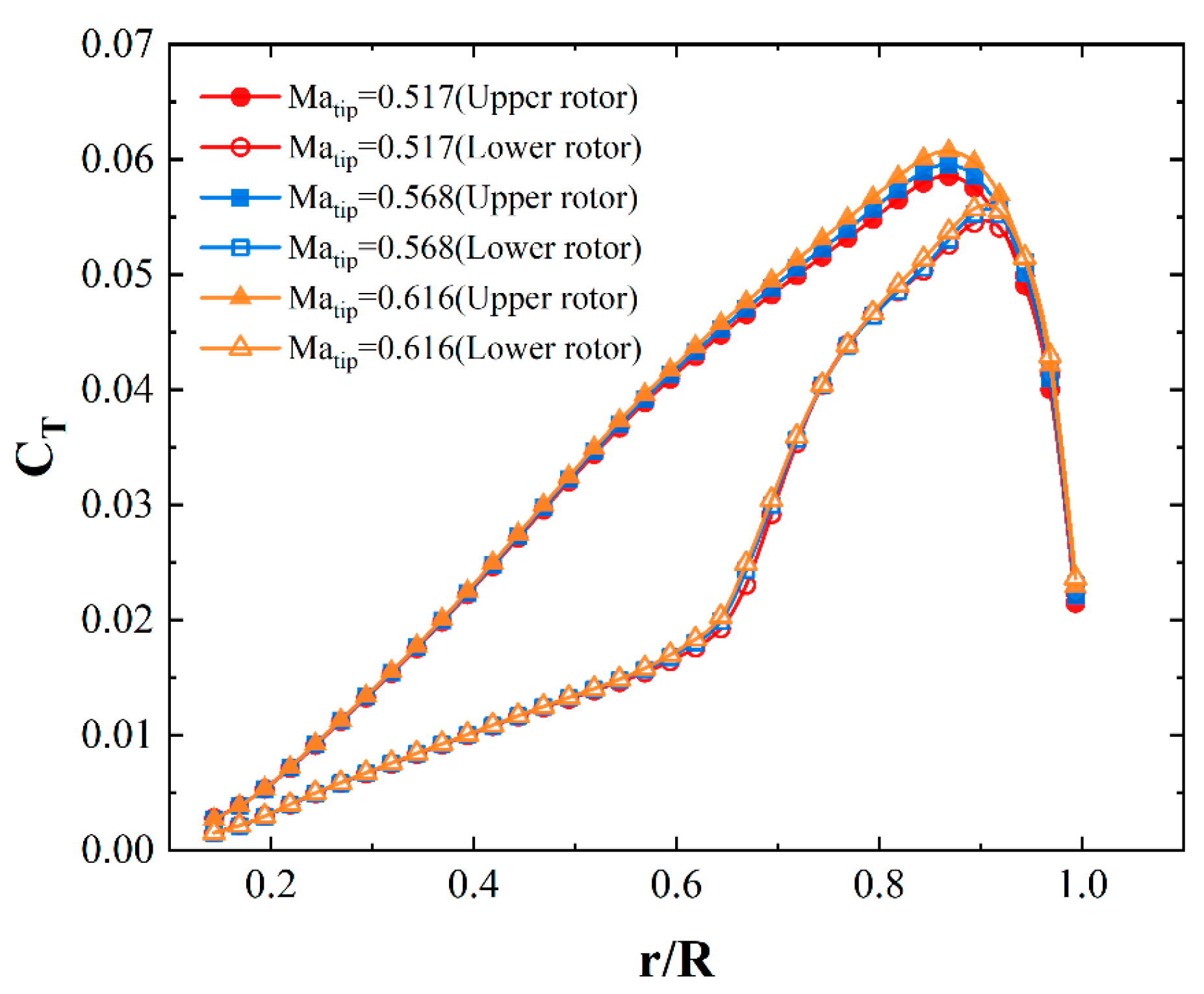
In this section, how rotational speed influences the BVI phenomenon is investigated while rotor spacing h/R is maintained at 0.438. Figure 9 displays the spanwise distribution of the thrust coefficient of the coaxial rotor at various rotational speeds when the azimuth gap between the two rotors is 90 degrees. The thrust coefficients of the upper rotor increased slightly as the rotational speed increased, and the curves of the spanwise thrust coefficients of the lower rotor at different rotational speeds were similar, indicating that the BVI phenomenon was almost not strengthened as the rotational speed increased.

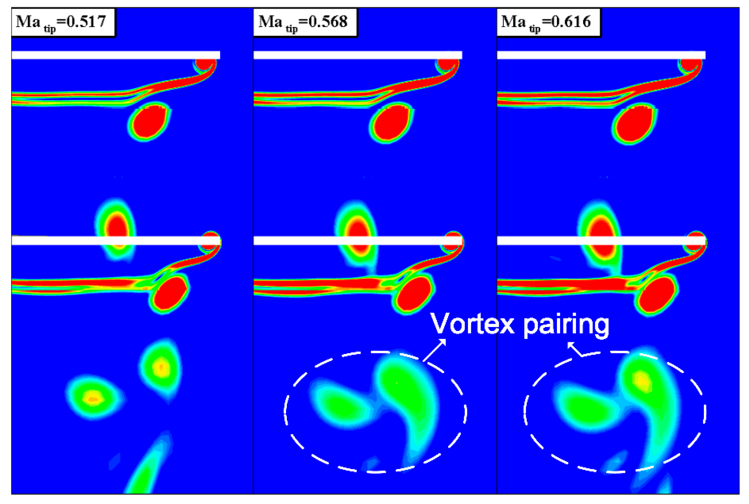
Figure 10 displays a comparison of two-dimensional wake plots at different rotational speeds when the azimuth gap is 90 degrees. The tip vortex of the upper rotor was strengthened as the rotational speed increased, and the vortex core moved downwards due to the acceleration of axial induced flow from the upper rotor. As rotational speed increased, the bound vortex of the lower rotor became stronger, resulting in a significant disruption to the tip vortex of the top rotor. As a result, the vortex structure of the top rotor became unstable after passing through the lower blade. Due to the strengthening of the tip vortex, the vortex of the top rotor and lower rotor were attracted to each other, resulting in vortex pairing.

Figure 11 shows the axial induced velocity distribution of a coaxial rotor’s horizontal section where the lower rotor is located at different rotational speeds. As the rotational speed increased, the area in the horizontal section where the tip vortex of the higher rotor was moved slightly away from the blade of the lower rotor so that tip vortex was less likely to affect the axial velocity of flow near the lower blade. However, the vorticity of the tip vortex increased as well, implying that the axial velocity of flow at a farther area can be accelerated by the vortex. Moreover, because of the increase in the lower rotor’s rotational speed, it needed a higher velocity of induced flow by vortex to change the local attack angle of the lower blade. Under the superposition of these influences, the effects caused by the BVI phenomenon on the spanwise load distribution of the lower rotor were similar when the rotating speed of the coaxial rotor increased.

3.3. Effect of Rotor Spacing

In this section, the influence of BVI to the thrust distribution and wake structure of coaxial rotors at different rotor spacing is analyzed, while the rotational speed, expressed as the tip-Mach number, remains at 0.517.

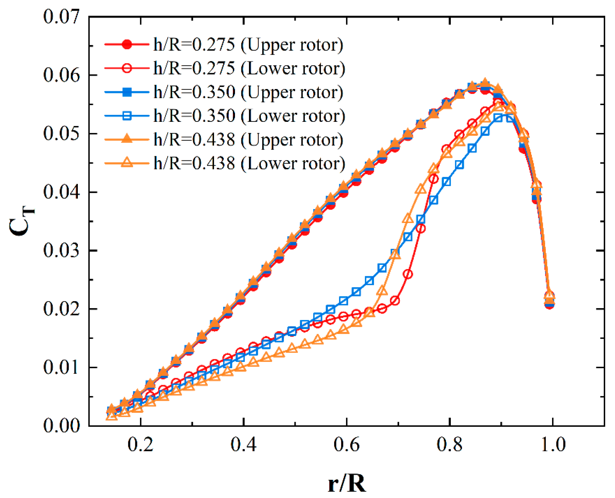
Figure 12 displays the spanwise distribution of thrust coefficient for coaxial rotors with different rotor spacings when the azimuth gap between the upper and lower rotors is 90 degrees. As the rotor spacing decreased, the thrust coefficient distribution of the upper rotor stayed constant, but the thrust distribution of the lower rotor fluctuated significantly around the range near 0.75 r/R, where the tip vortex of the upper rotor passed across the lower blade. When the spacing was 0.438, there was an S-shape fluctuation in the curve of thrust coefficient distribution which was caused by the BVI. As rotor spacing decreased to 0.275, the location of S-shaped fluctuations on the curve moved closer to the tip of the blade. However, when the rotor spacing reached 0.35, the thrust coefficient gradient reduced and the curve returned to a smooth shape, indicating that the BVI phenomena did not exist at this azimuth.

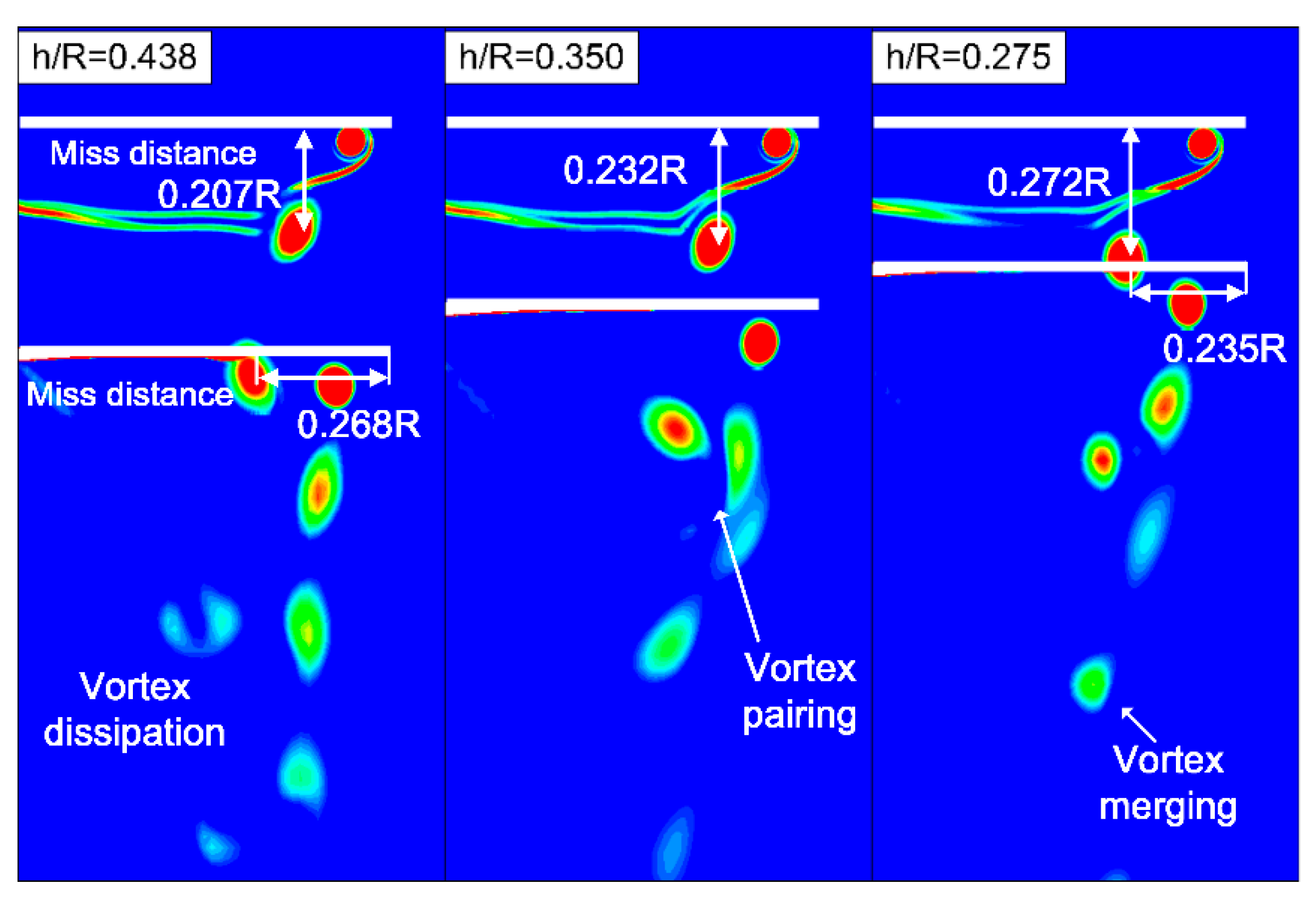
Figure 13 shows the vorticity magnitude contours in the vertical slice where the lower blades are located at different rotor spacings. Note the miss distance between the vortex and blade can be divided into axial miss distance and spanwise miss distance. The axial miss distance is defined as the vertical distance from vortex core to the horizontal section where the upper rotor is located. The spanwise miss distance is defined as the horizontal distance from the vortex to the tip of blade. With a decrease in rotor spacing, the suction from the lower rotor is strengthened, the blade-tip vortex of the upper rotor moves downwards significantly, and its axial miss distance of vortex increases. The vortex of the upper blade meets the lower blade sooner, which means the vortex takes less time to develop after being generated from the tip of the upper blade and before meeting the lower blade. As a result, the upper rotor’s spiral wake is shorter, and the viscous dissipation of the vortex decreases, resulting in a greater vortex strength as the vortex meets the lower blade, and in a stronger BVI phenomenon. Then, due to the decrease in rotor spacing, the vortex from the upper rotor does not have sufficient time to shrink before interacting with the blade of the lower rotor, and its miss distance is small. Thus, the position of BVI changes and moves closer to the tip of the blade. Because of the vortex’s high vorticity and the close distance between two vortexes, there is a stronger attraction between two vortexes, resulting in the vortex pairing and vortex merging phenomena.

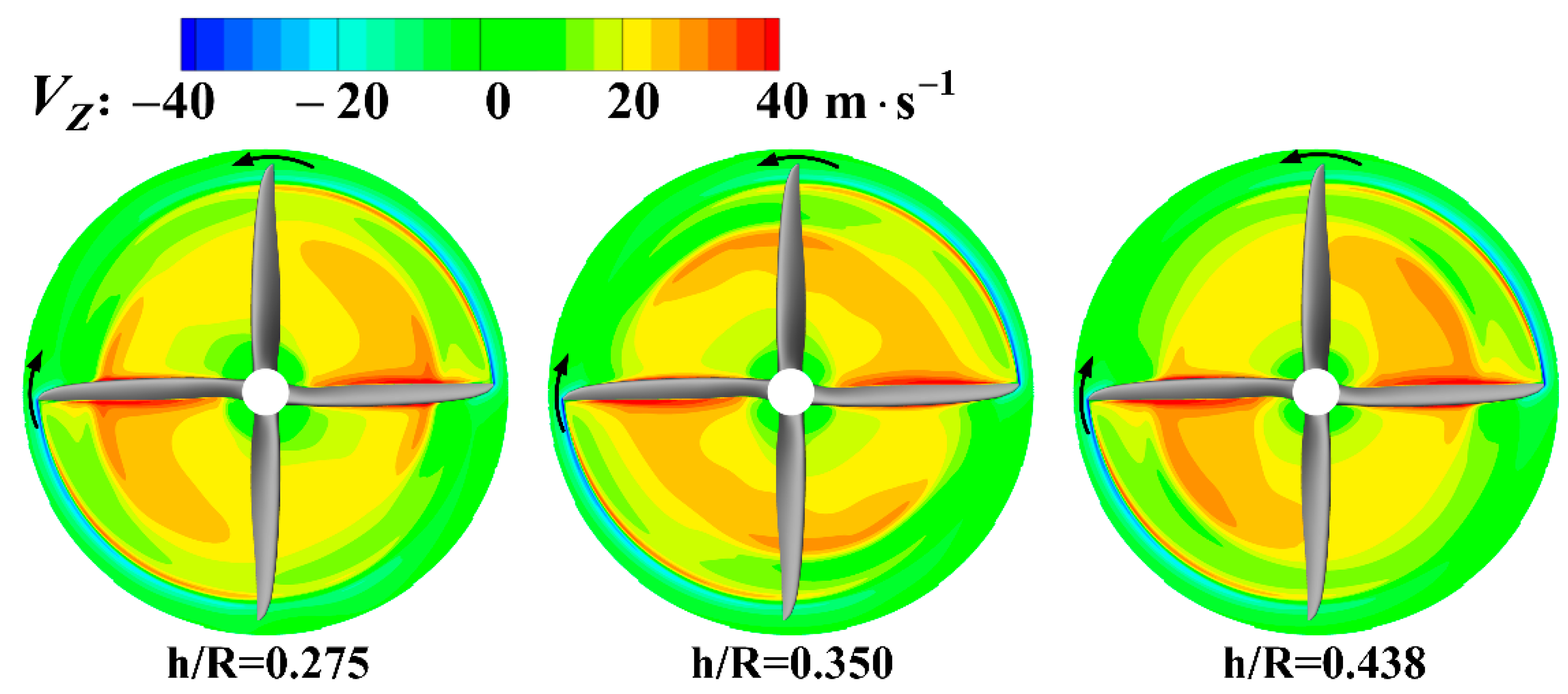
Figure 14 displays the axial induced velocity distribution of a coaxial rotor at the horizontal section where the lower rotors are located at different rotor spacings. It is shown that the region influenced by the tip vortex of the higher rotor changes as rotor spacing decreases. As a result of the 0.438 and 0.275 rotor spacing, the region the tip vortex of the upper rotor passes through is close to the blade as the BVI phenomena occurs. When the rotor spacing is 0.35, the region the tip vortex of the upper rotor passes through is far away from the blade so the BVI phenomenon does not appear at this azimuth.

4. Conclusions

This paper used CFD techniques based on uRANS solver, which has been verified by experiments, to investigate how azimuth gap, rotating speed, and rotor spacing affect the BVI phenomenon of a coaxial rigid rotor, which may be useful in eVTOL design. The conclusions can be derived as follows:

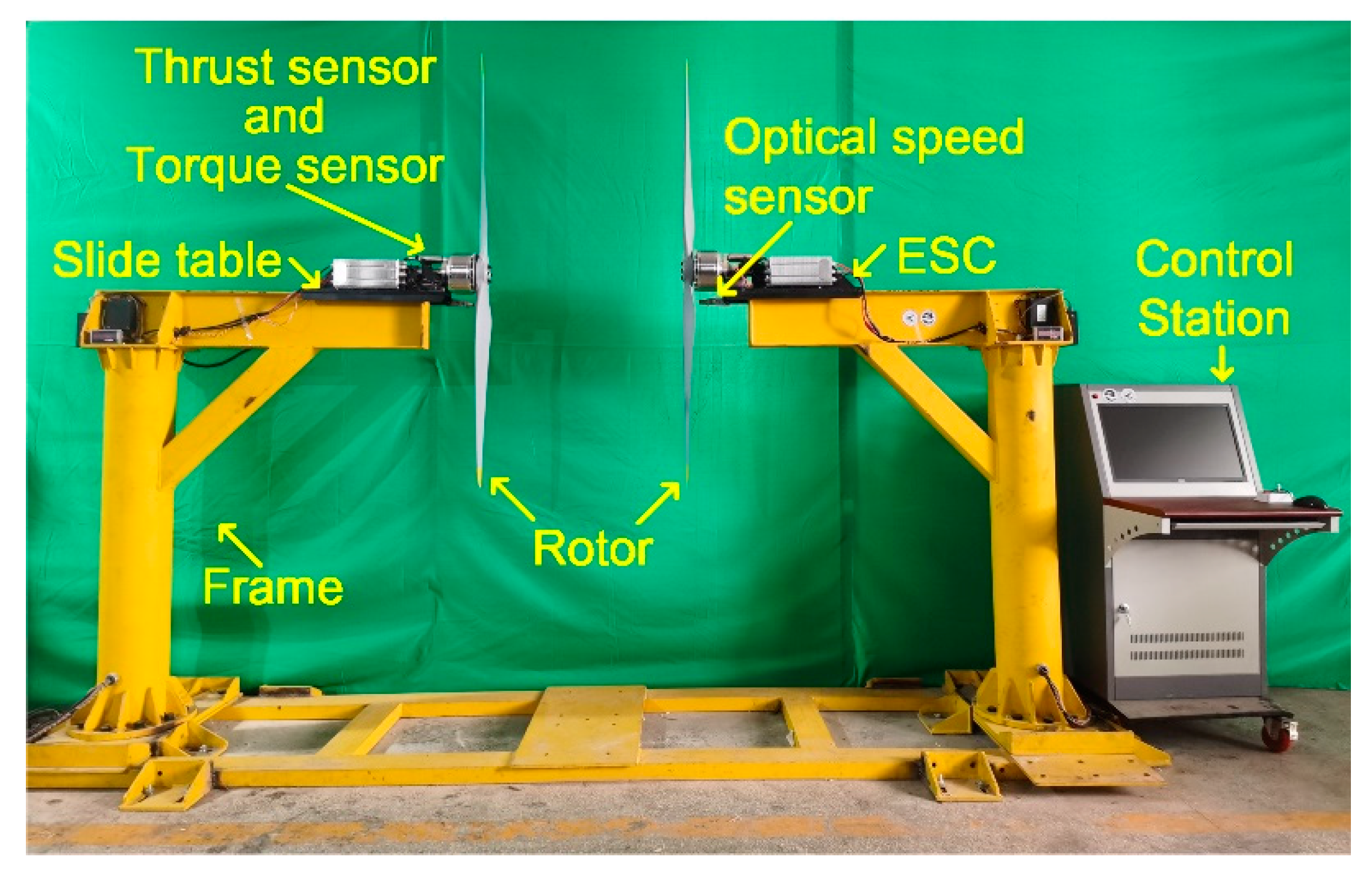
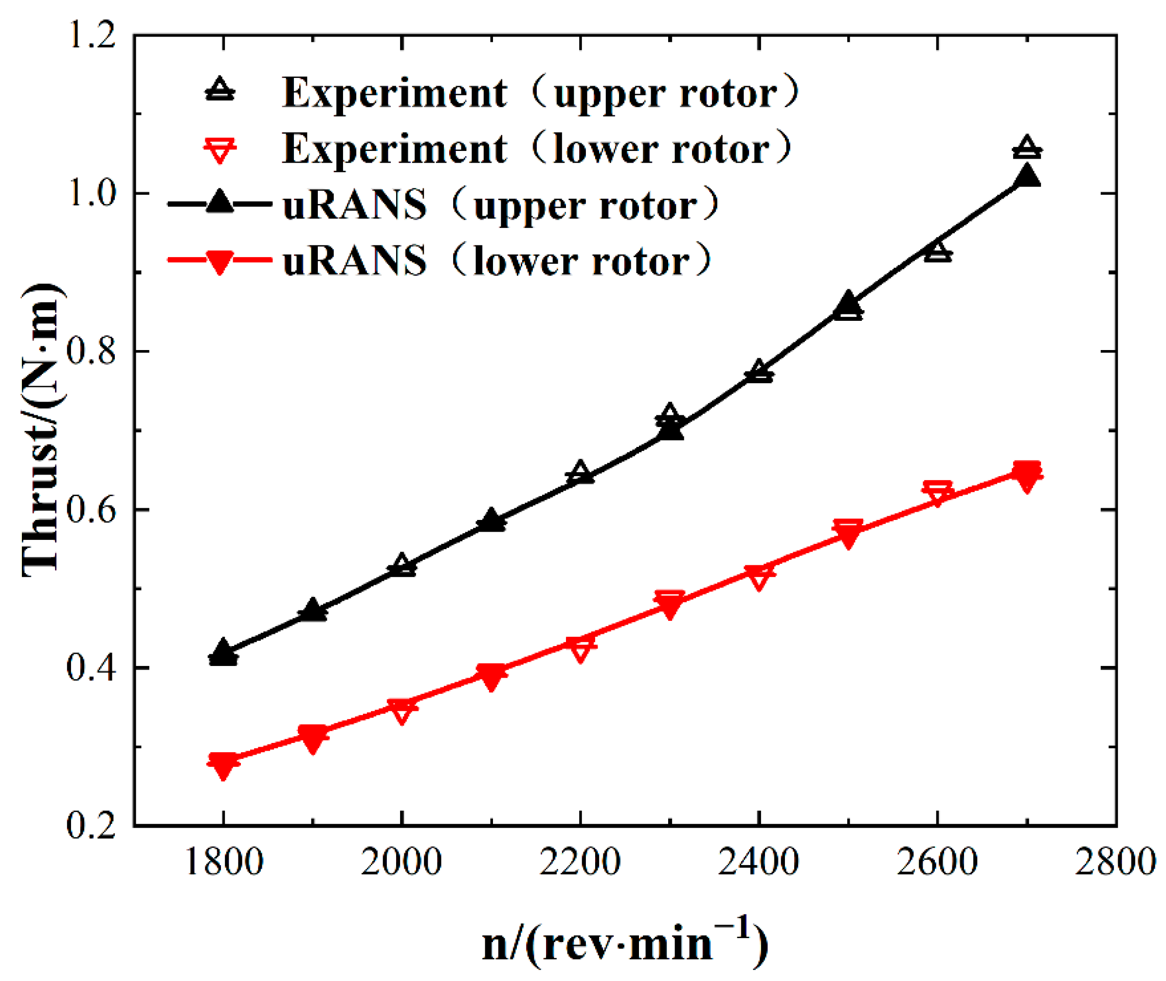
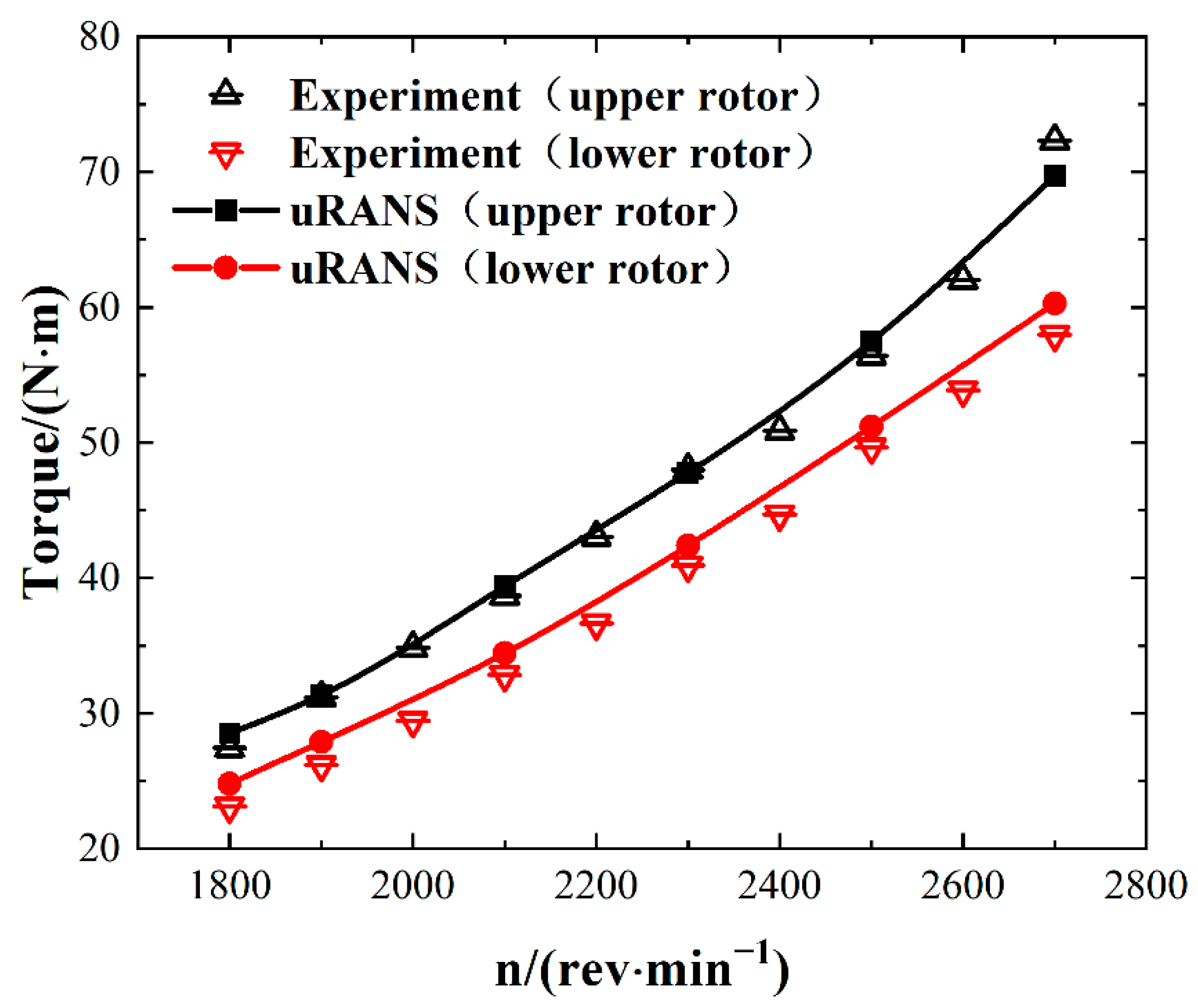
• The validation of the CFD method employing the used uRANS solver combined with sliding mesh technology to simulate the motion of a coaxial system has been verified by a one-to-one experiment. The thrust and torque of each rotor in a coaxial system can be predicted accurately using this method.
• The BVI phenomenon always occurs in a particular range of azimuth gap when the tip vortex of the upper rotor is close to the blade of the lower rotor. As the BVI phenomenon occurs, the tip vortex of the upper rotor will influence the axial induced flow near the lower blade and alter the spanwise thrust coefficient distribution of the lower rotor, resulting in an S-shaped fluctuation on the thrust coefficient curve. When the BVI phenomenon occurs, the surface and bound vortex will also impact the stability of the vortex structure of the upper rotor and accelerate its dissipation.
• As the rotational speed increases, the vortex cores of the upper rotor descend and move away from the lower blade, whereas the vorticity strength of the vortex increases. The two effects counteract each other, resulting in a small change in BVI. At different rotational speeds, the spanwise distribution of thrust coefficient on the lower blade is similar.
• As the rotor spacing decreases, the position of the upper rotor’s vortex core changes significantly: the axial miss distance increases, and the spanwise miss distance reduces. The BVI phenomenon gains strength and its position moves close to the tip of the lower blade. Because of the decrease in spanwise miss distance, the tip vortices from the two rotors approach each other, resulting in vortex pairing and vortex merging.

As a concluding remark, the present work simulated the motion of a coaxial rotor at different azimuth gaps, rotational speeds, and rotor spacing, and discussed the effect of these variables on the BVI phenomenon. It is hoped that the results of this research will offer guidance to select a reasonable configuration while using the coaxial rotor system in eVTOL design.

References

1. Diaz, P.V.; Rubio, R.C.; Yoon, S. Simulations of Ducted and Coaxial Rotors for Air Taxi Op-erations. In Proceedings of the AIAA Aviation 2019 Forum, Dallas, TX, USA, 17–21 June 2019. [Google Scholar] [CrossRef]
2. Kadhiresan, A.R.; Duffy, M.J. Conceptual Design and Mission Analysis for eVTOL Urban Air Mobility Flight Vehicle Configurations. In Proceedings of the AIAA Aviation 2019 Forum, Dallas, TX, USA, 17–21 June 2019. [Google Scholar] [CrossRef]
3. Tinney, C.E.; Valdez, J. Thrust and Acoustic Performance of Small-Scale, Coaxial, Corotat-ing Rotors in Hover. AIAA J. 2020, 58, 1657–1667. [Google Scholar] [CrossRef]
4. Qi, H.; Wang, P.; Jiang, L.; Zhang, Y. Investigation on Aerodynamic Noise Characteristics of Coaxial Rotor in Hover. Appl. Sci. 2022, 12, 2813. [Google Scholar] [CrossRef]
5. Chang, M.; Feng, X.; Zhang, Y.; Zhang, X.; Bai, J.Q. Flow analysis on the ventral gap of a paper airplane. Proc. Inst. Mech. Eng. Part C J. Mech. Eng. Sci. 2020. [Google Scholar] [CrossRef]
6. Zhang, Y.; Zhang, X.; Li, Y.; Chang, M.; Xu, J. Aerodynamic performance of a low-Reynolds UAV with leading-edge protuberances inspired by humpback whale flippers. Chin. J. Aeronaut 2021, 34, 415–424. [Google Scholar] [CrossRef]
7. Singh, R.; Hao, K.; Cameron, C.; Sirohi, J. Computational and Experimental Investigations of Coaxial Rotor Unsteady Loads. In Proceedings of the 54th AIAA Aerospace Sciences Meeting, San Diego, CA, USA, 4–8 January 2016. [Google Scholar] [CrossRef]
8. Singh, R.; Hao, K.; Sirohi, J. Computational Investigations of Transient Loads and Blade Deformations on Coaxial Rotor Systems. In Proceedings of the 33rd AIAA Applied Aerodynamics Conference, Dallas, TX, USA, 22–26 June 2015. [Google Scholar] [CrossRef]
9. Dobrzynski, W. Propeller Noise Reduction by Means of Unsymetrical Blade-Spacing. J. Sound Vib. 1993, 163, 123–136. [Google Scholar] [CrossRef]
10. Walsh, G.; Brentner, K.; University, T.; Jaco-bellis, G.; Gandhi, F.; Institute, R.P. An Acoustic Investigation of a Coaxial Helicopter in High-Speed Flight. In Proceedings of the AHS 72nd Annual Forum, West Palm Beach, FL, USA, 17–19 May 2016. [Google Scholar]
11. Harrington, R.D. Full-Scale-Tunnel Investigation of the Static-Thrust Performance of a Coaxial Helicopter Rotor; NACA: Washington, DC, USA, 1951. [Google Scholar]
12. Landgrebe, A.J.; Bellinger, E.D. Experimental investigation of model variable-geometry and ogee tip rotors. In Proceedings of the 29th Annual National Forum of the American Helicopter Society, (No. AHS PREPRINT 703), Washington, DC, USA, 9–11 May 1973. [Google Scholar]
13. Ramasamy, M. Measurements comparing hover performance of single, coaxial, tandem, and tilt-rotor configurations. In Proceedings of the AHS 69th Annual Forum, Phoenix, AZ, USA, 24–28 May 2013. [Google Scholar]
14. Gordon, L.J.; Monica, S. Figure of Merit Definition for Coaxial Rotors. J. Am. Helicopter Soc. 2008, 53, 290–300. [Google Scholar]
15. Kim, H.W. A Comparison of Coaxial and Conventional Rotor Performance. J. Am. Helcopter Soc. 2010, 55, 012004. [Google Scholar] [CrossRef]
16. Tan, J.; Sun, Y.; Barakos, G.N. Unsteady loads for coaxial rotors in forward flight computed using a vortex particle method. Aeronaut. J. 2018, 122, 693–714. [Google Scholar] [CrossRef] [Green Version]
17. Lakshminarayan, V.K.; Baeder, J.D. Computational Investigation of Microscale Coaxial Rotor Aerodynamics in Hover. J. Aircr. 2009, 47, 940–955. [Google Scholar] [CrossRef] [Green Version]
18. Ko, J.; Lee, S. Numerical Investigation of Inter-Rotor Spacing Effects on Wake Dynamics of Coaxial Rotors. J. Aircr. 2021, 58, 363–373. [Google Scholar] [CrossRef]
19. Qi, H.; Xu, G.; Lu, C.; Shi, Y. A study of coaxial rotor aerodynamic interaction mechanism in hover with high-efficient trim model. Aerosp. Sci. Technol. 2019, 84, 1116–1130. [Google Scholar] [CrossRef]
20. Bauer, R.L.; Thomas, C.J.; Baker, E.V.P.; Johnson, E.M.; Williams, K.R.; Langenderfer, M.J.; Johnson, C.E. Shock wave formation from head-on collision of two subsonic vortex rings. Sci. Rep. 2022, 12, 7492. [Google Scholar] [CrossRef] [PubMed]
21. Lim, T.T.; Nickels, T.B. Instability and Reconnection in the Head-On Collision of Two Vortex Rings. Nature 1992, 357, 225–227. [Google Scholar] [CrossRef]
22. New, T.H.; Shi, S.; Zang, B. Some observations on vortex-ring collisions upon inclined surfaces. Exp. Fluids 2016, 57, 109. [Google Scholar] [CrossRef]
23. Jasak, H.; Weller, H.G.; Gosman, A.D. High resolution NVD differencing scheme for arbi-trarily unstructured meshes. Int. J. Numer. Meth. Fluids. 1999, 31, 431–449. [Google Scholar] [CrossRef]
24. Menter, F.R. Zonal Two Equation k-w Turbulence Models For Aerodynamic Flows. In Proceedings of the 23rd Fluid Dynam-ics, Plasmadynamics, and Lasers Conference, Orlando, FL, USA, 6–9 July 1993. [Google Scholar]
25. Mangler, K.; Smith, J. Behaviour of the Vortex Sheet at the Trailing Edge of a Lifting Wing. Aeronaut. J. 1968, 74, 906–908. [Google Scholar] [CrossRef]
Figure 1. Boundary condition for a two-blade coaxial rotor and its computational mesh.
Energies 15 07761 g001
Figure 2. The experimental setup arranged in coaxial rotor configuration with sensors.
Energies 15 07761 g002
Figure 3. Model and geometry characters of rotor.
Energies 15 07761 g003
Figure 4. Performance comparison between experimental and numerical calculation data of coaxial rotor.
Energies 15 07761 g004aEnergies 15 07761 g004b
Figure 5. Sketch map of rotor blade locations.
Energies 15 07761 g005
Figure 6. Spanwise distribution of thrust coefficient of coaxial rotor at different azimuthal angles. (The blade-tip Mach number was 0.517, the rotor spacing d/R was 0.438.)
Energies 15 07761 g006
Figure 7. Vorticity magnitude contours when rotors were at different azimuthal angles (the blade-tip Mach number was 0.517, the rotor spacing d/R was 0.438).
Energies 15 07761 g007
Figure 8. Axial induced velocity contours at the horizontal section where the lower rotor is located at different azimuth gaps (the rotation direction of upper rotor is counter-clockwise and the rotation direction of lower rotor is clockwise).
Energies 15 07761 g008
Figure 9. Spanwise distribution of thrust coefficient for coaxial rotor at different rotational speeds.
Energies 15 07761 g009
Figure 10. Comparison of two-dimensional wake plots at different rotational speeds for coaxial rotor at 45 degree section (the azimuth gap between the two rotors is 90 degrees).
Energies 15 07761 g010
Figure 11. Axial induced velocity contours at the horizontal section of the lower rotor at different rotor spacings (the rotation direction of upper rotor is counter-clockwise and the rotation direction of lower rotor is clockwise).
Energies 15 07761 g011
Figure 12. Spanwise distribution of thrust coefficient for coaxial rotor in different rotor spacings when phase difference between upper and lower rotor is 90 degrees (the blade-tip Mach number is 0.517).
Energies 15 07761 g012
Figure 13. Comparison of two-dimensional wake plots with different rotor spacing for coaxial rotor when azimuth gap is 90 degrees (the blade-tip Mach number is 0.517).
Energies 15 07761 g013
Figure 14. Axial induced velocity contours at the horizontal section where the lower rotor is located at different rotor spacings (the rotation direction of upper rotor is counter-clockwise and the rotation direction of lower rotor is clockwise).
Energies 15 07761 g014
Publisher’s Note: MDPI stays neutral with regard to jurisdictional claims in published maps and institutional affiliations.