

Robust Sensorless Control of Interior Permanent Magnet Synchronous Motor Using Deadbeat Extended Electromotive Force Observer


Abstract
:1. Introduction
2. The EEMF Estimation Algorithm
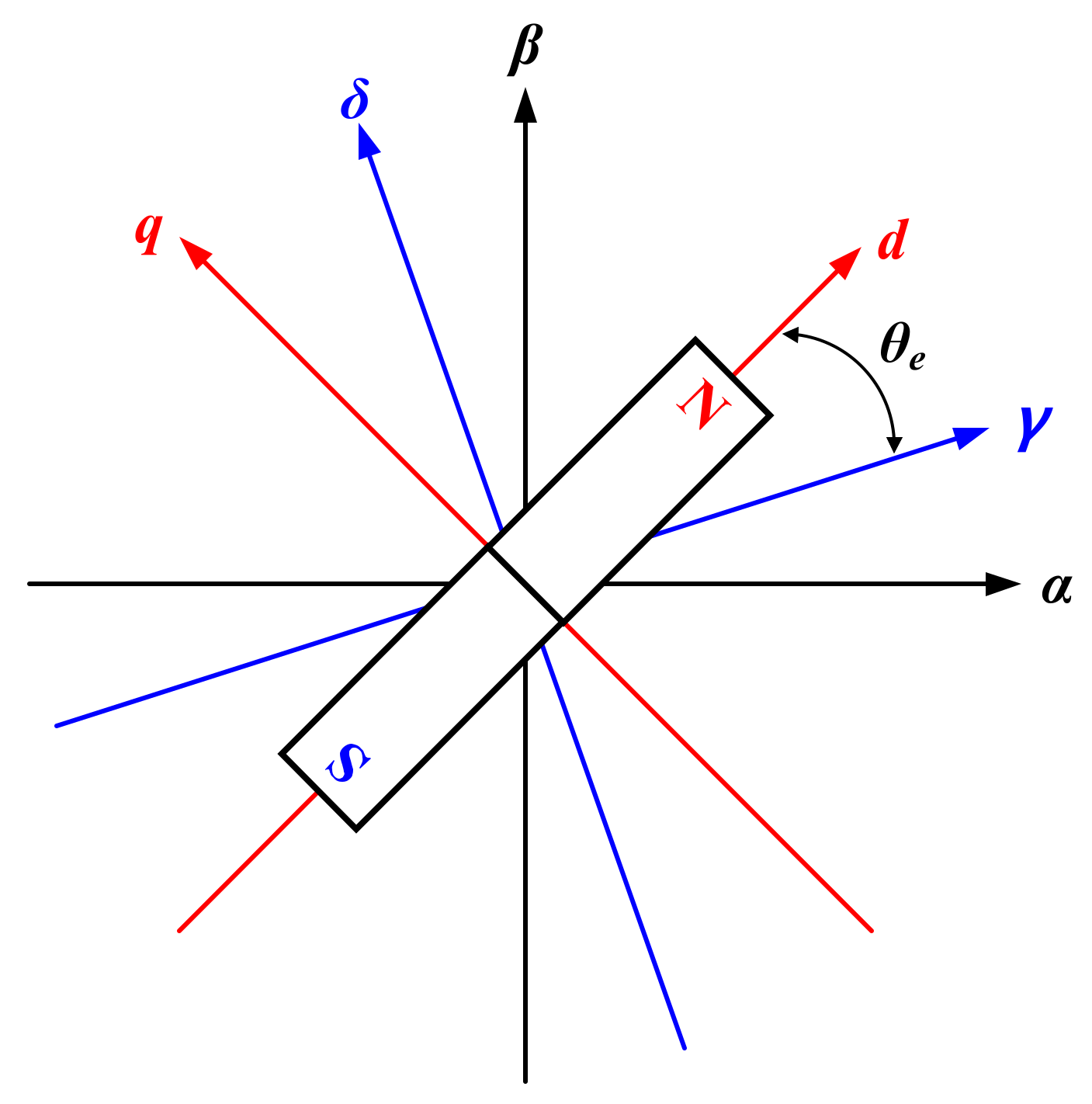
2.1. Mathematical Model of IPMSM
2.2. EEMF Estimation Using Reconstructor
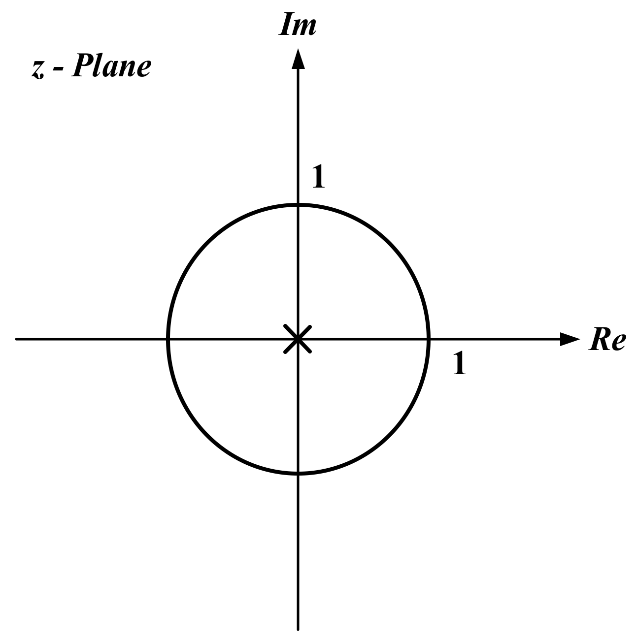
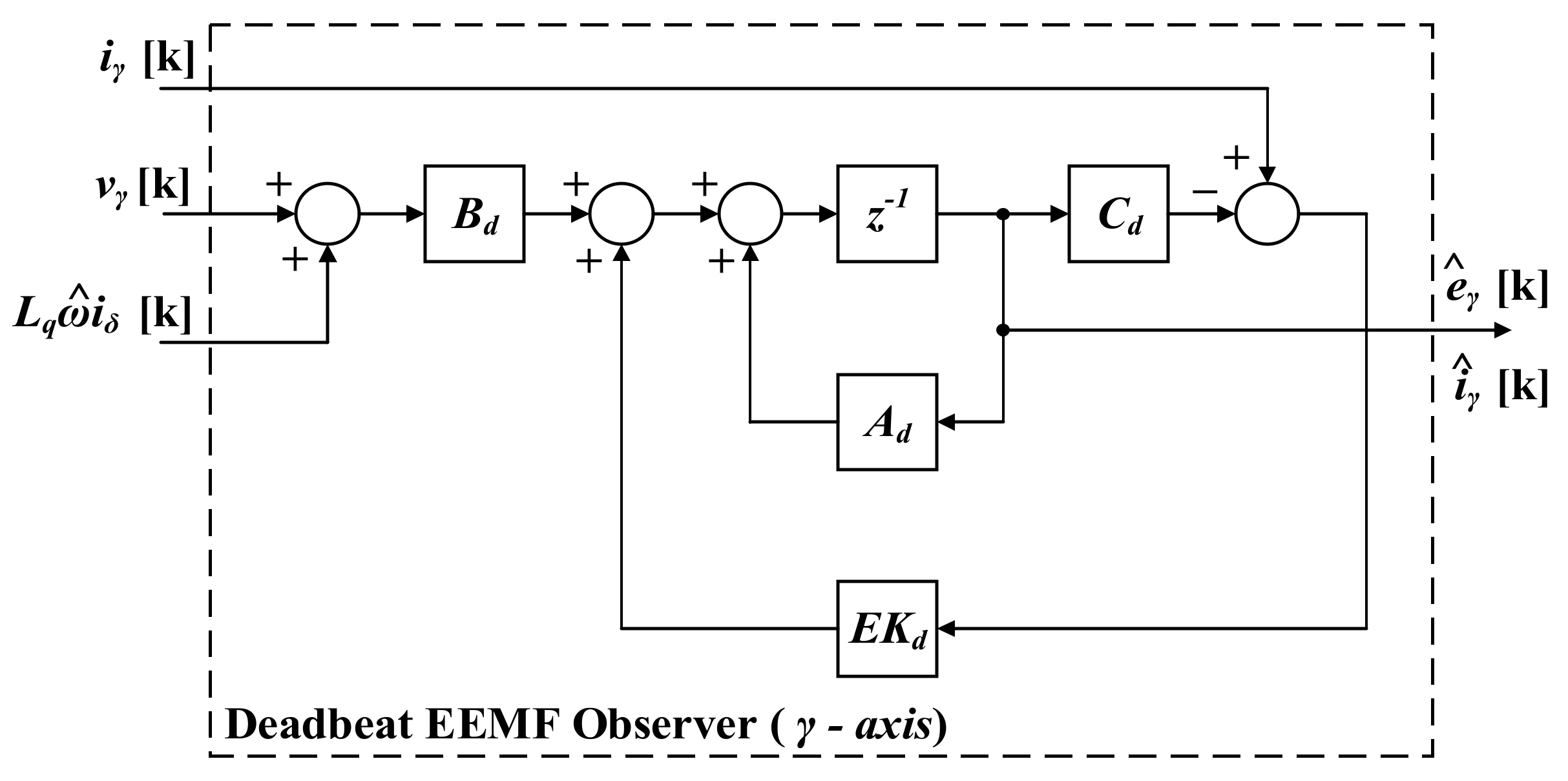
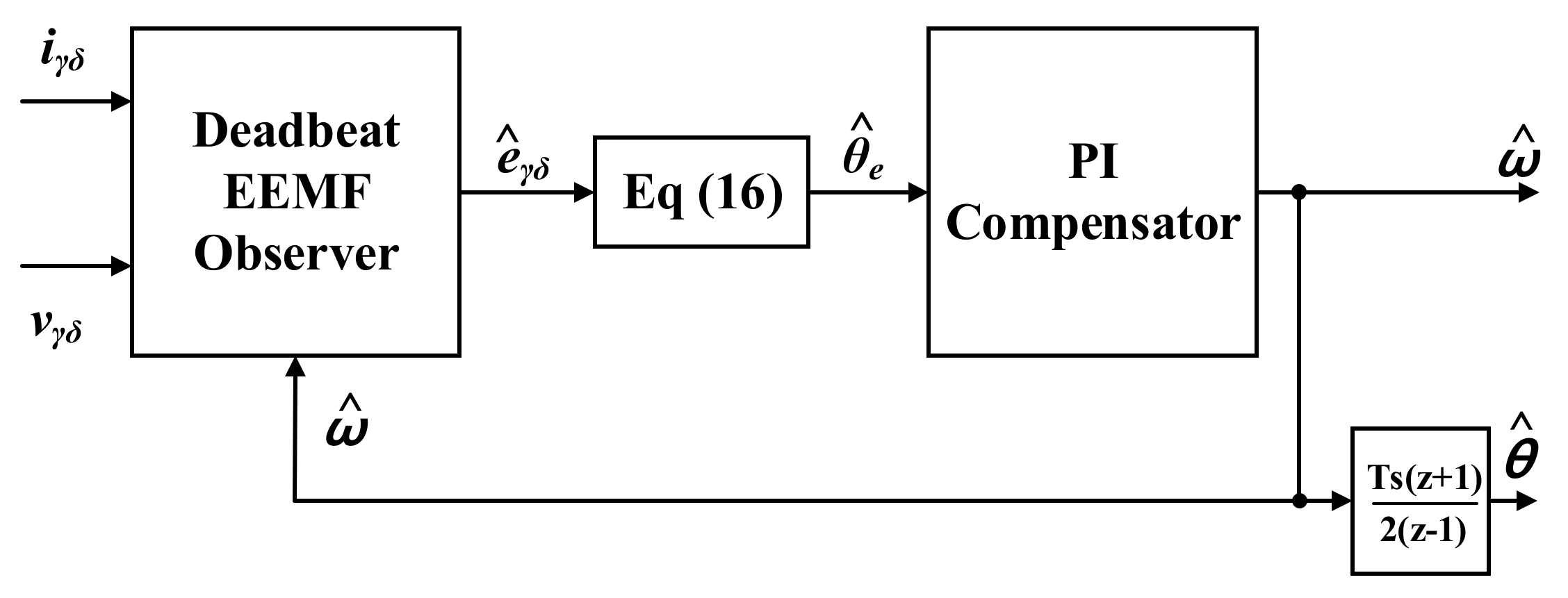
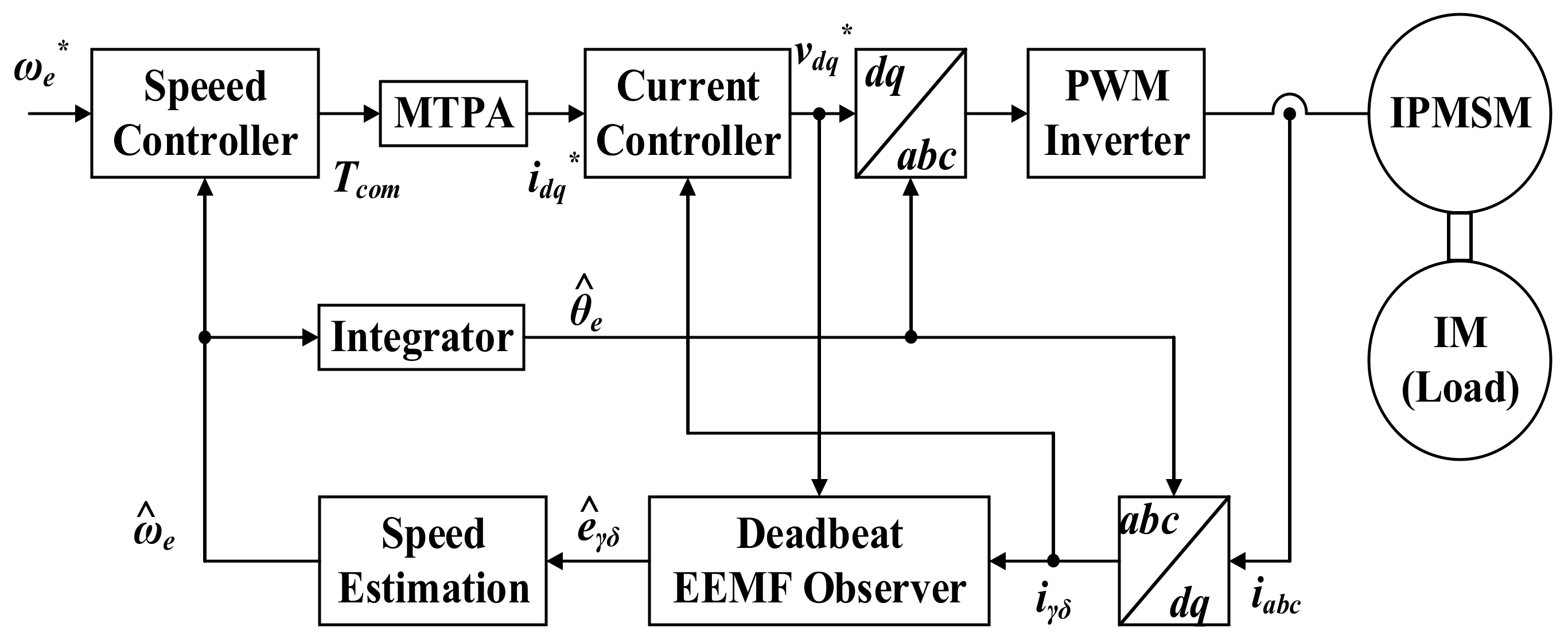
2.3. Proposed Deadbeat EEMF Observer
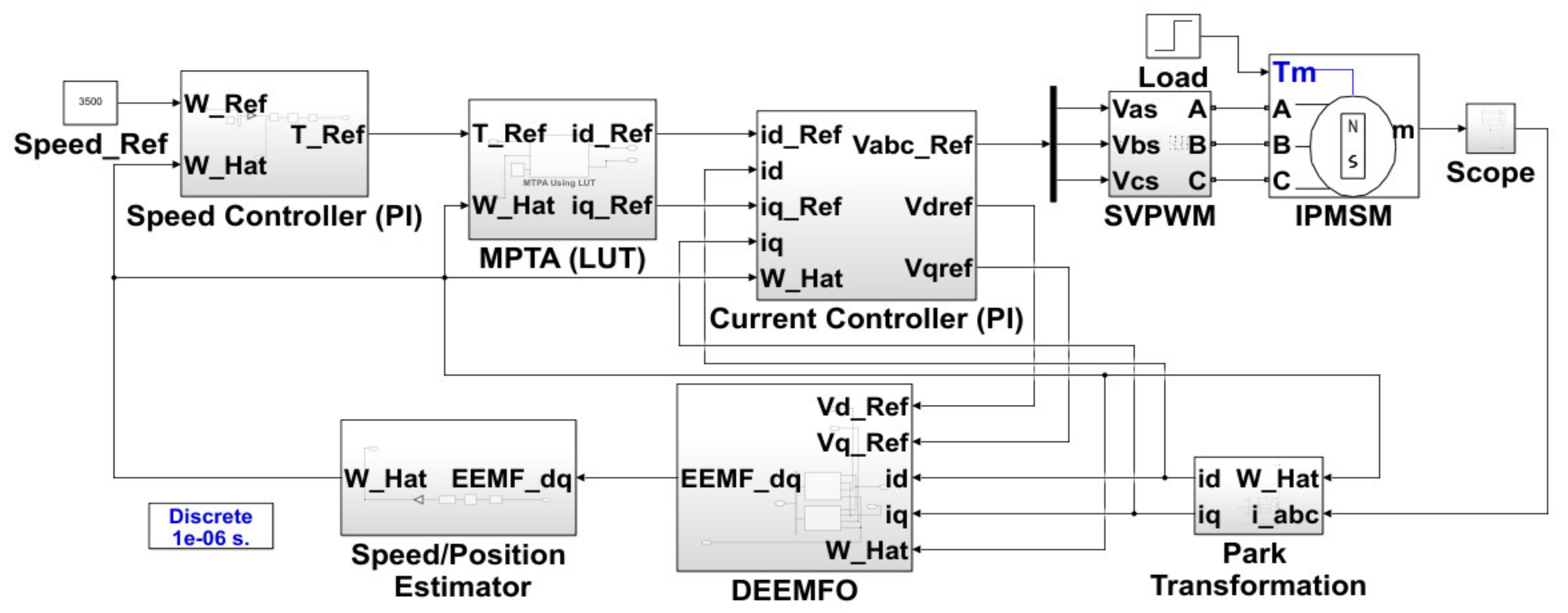
3. Simulation
3.1. Set-Up
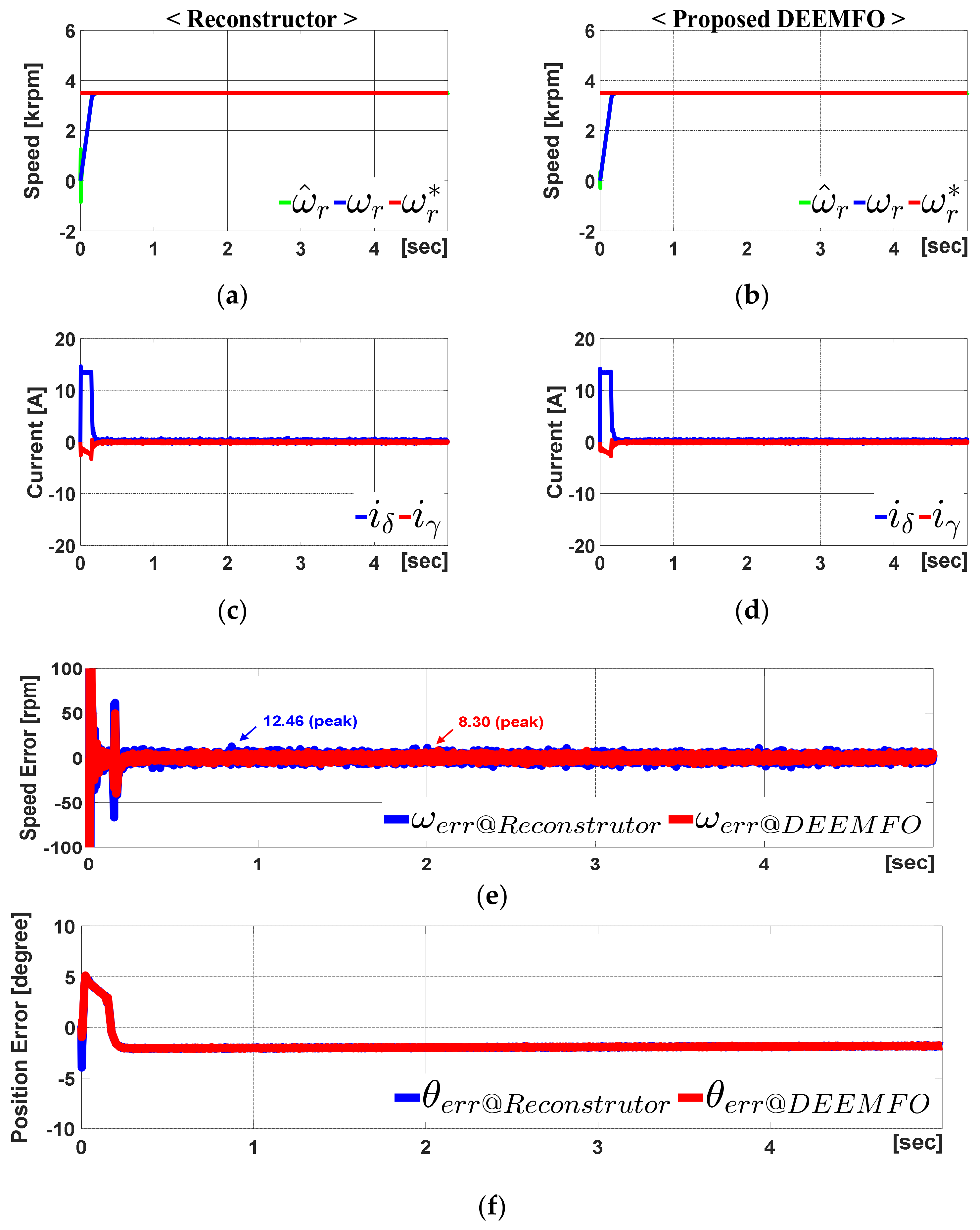
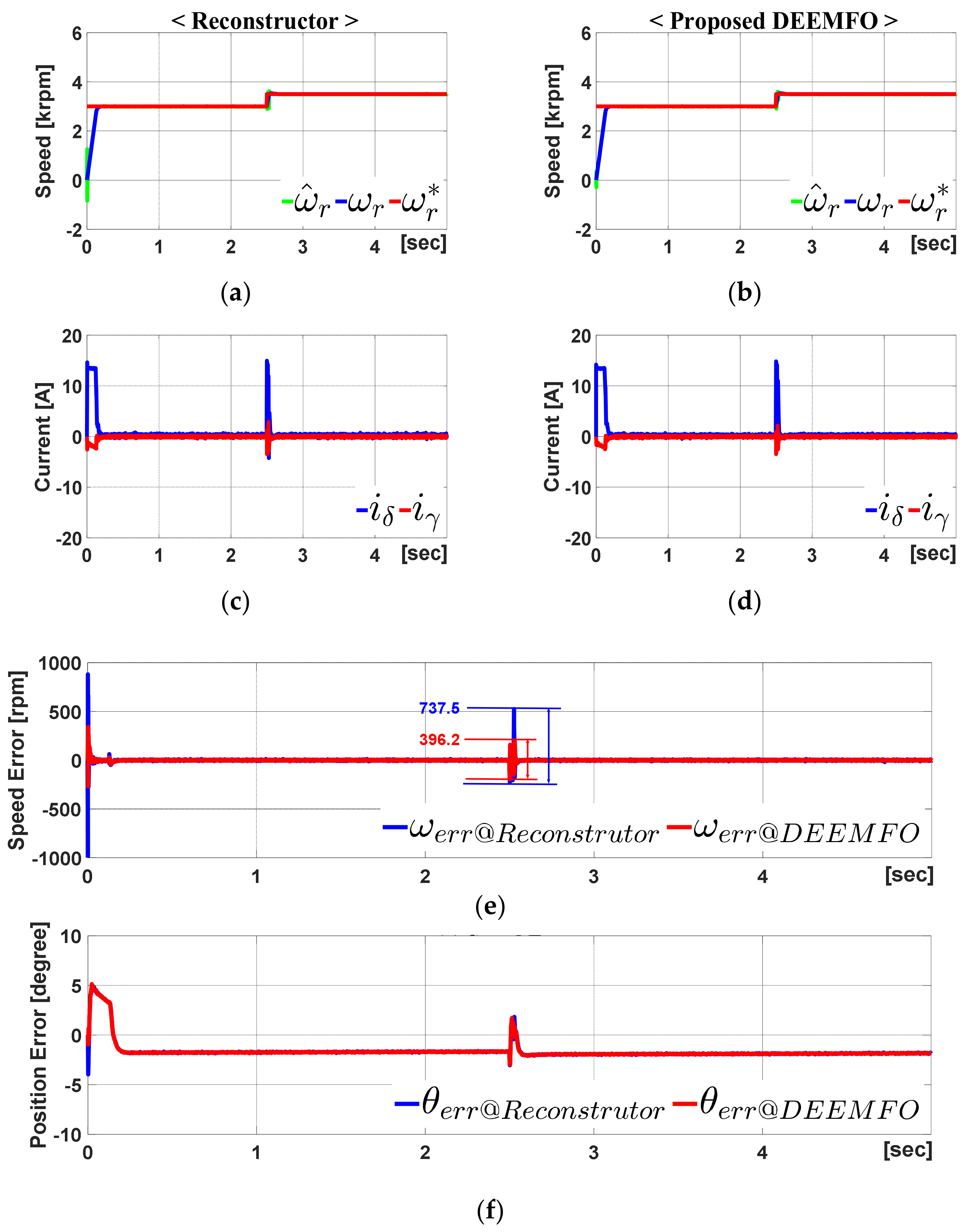
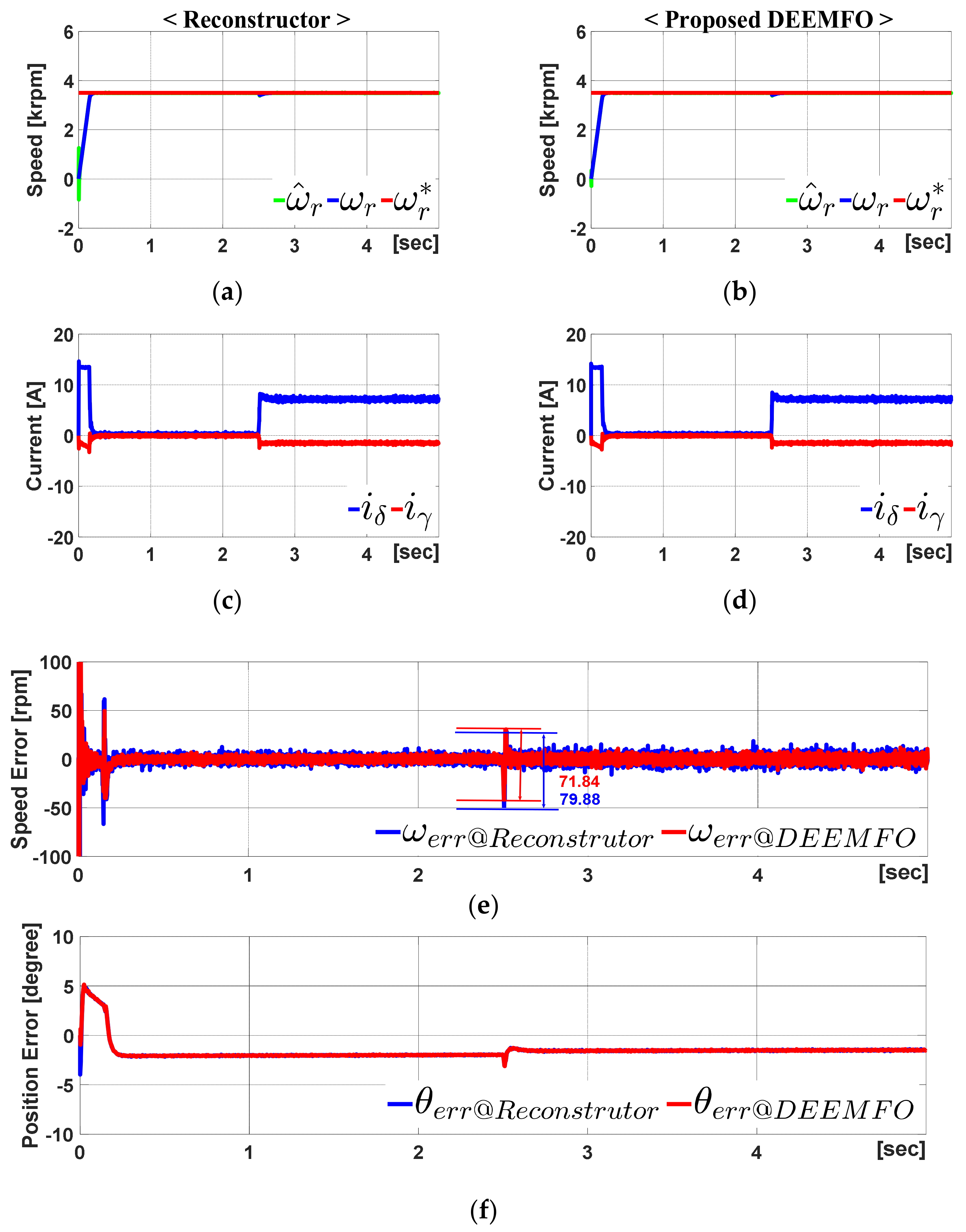
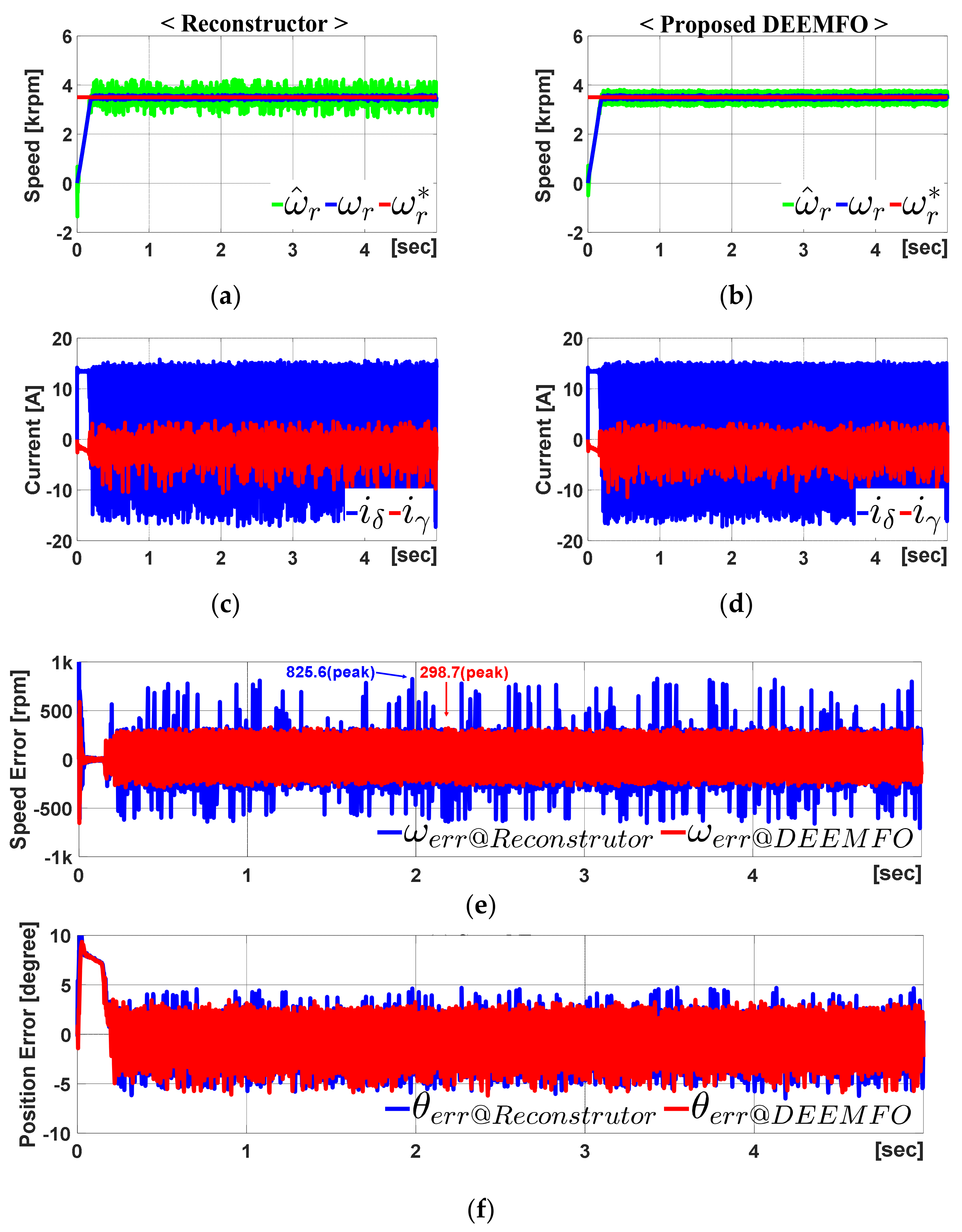
3.2. Simulation Result
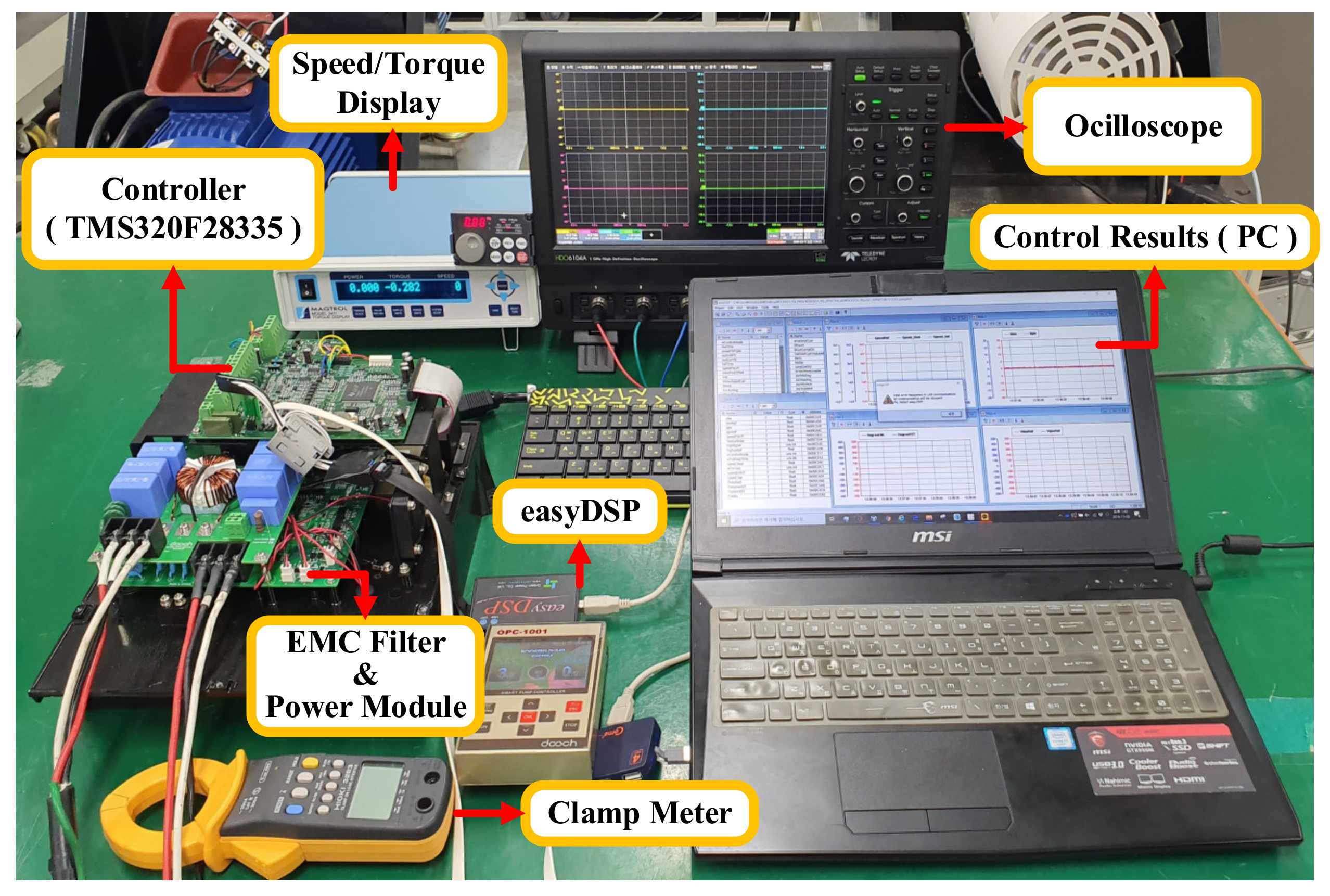
4. Experiment
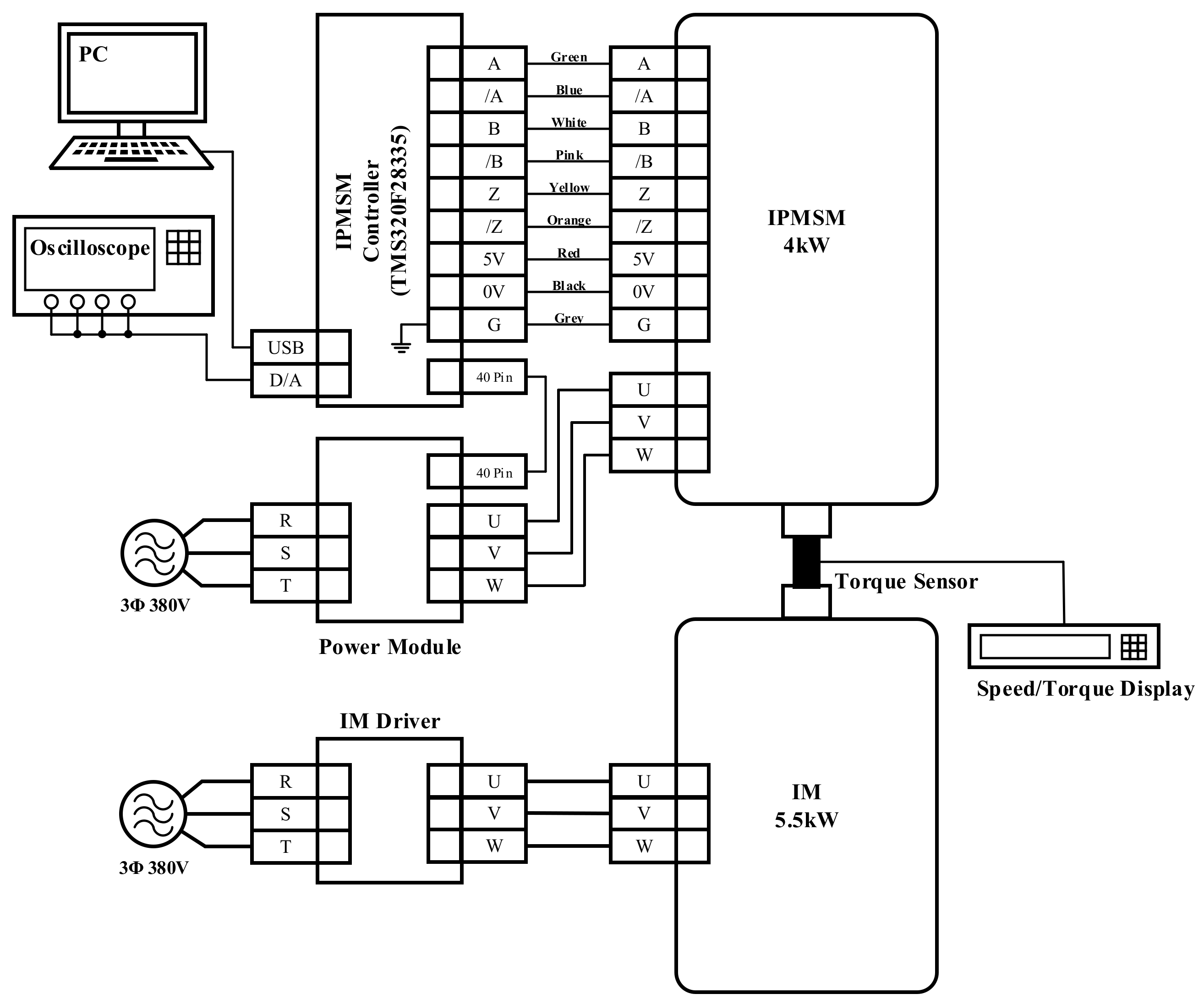
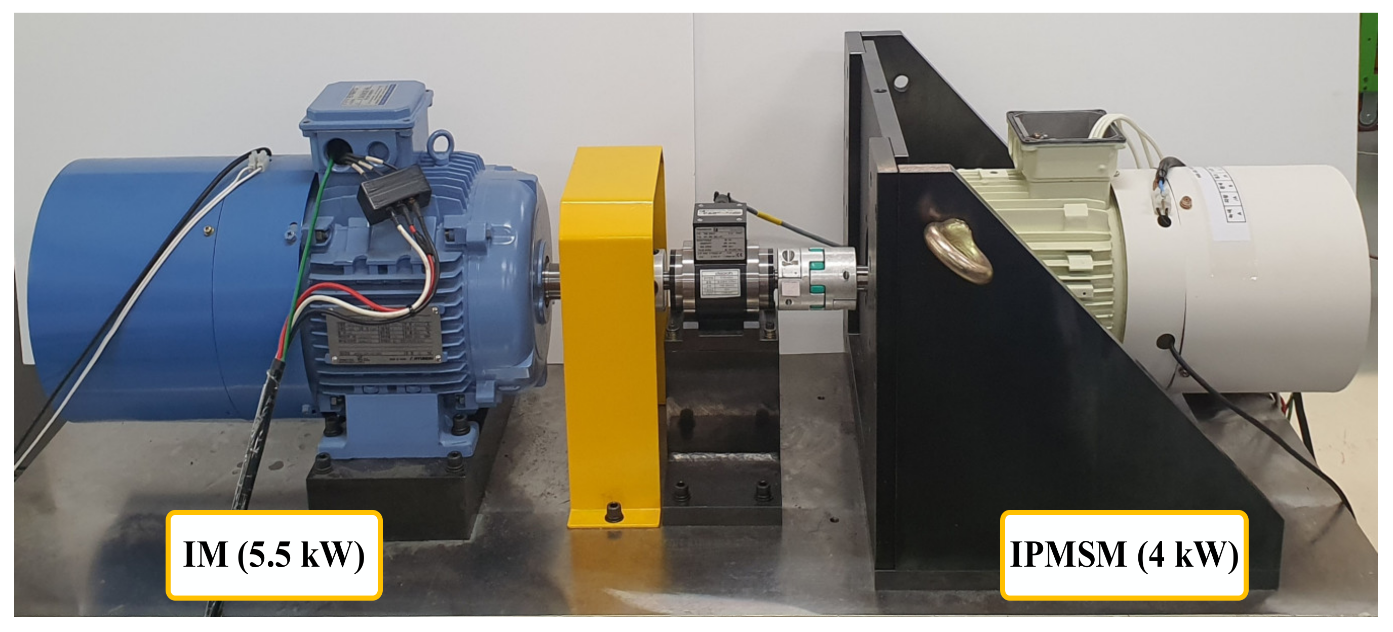
4.1. Set-Up
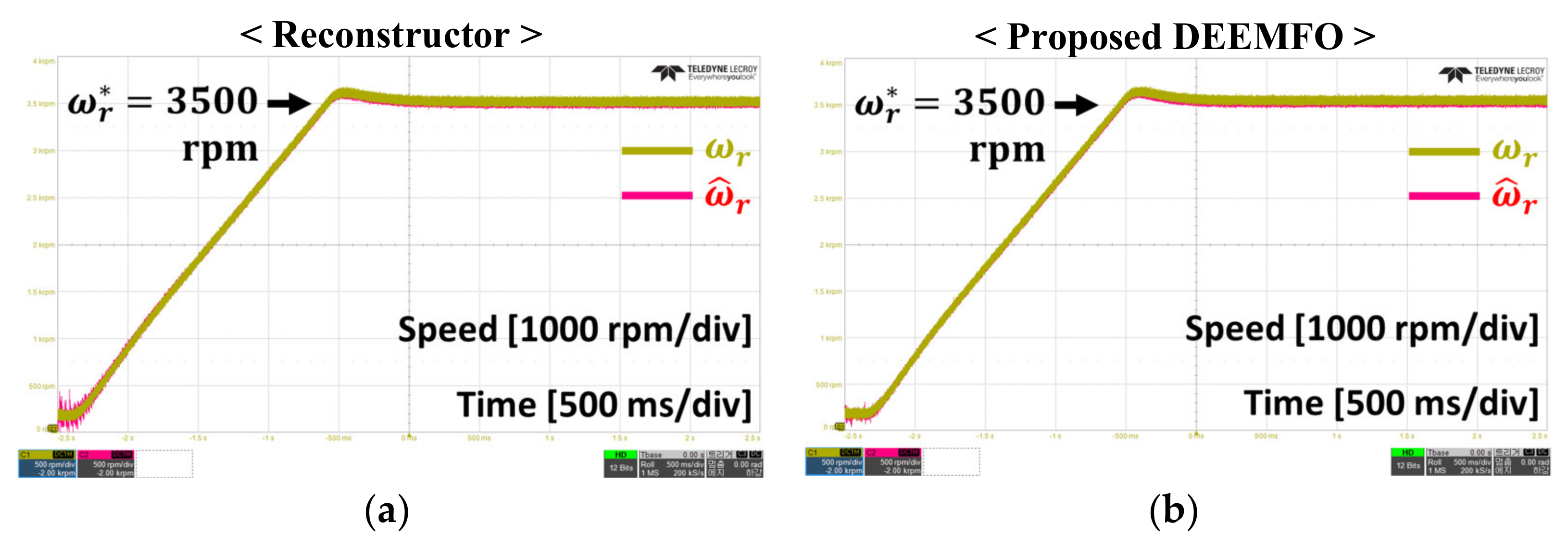
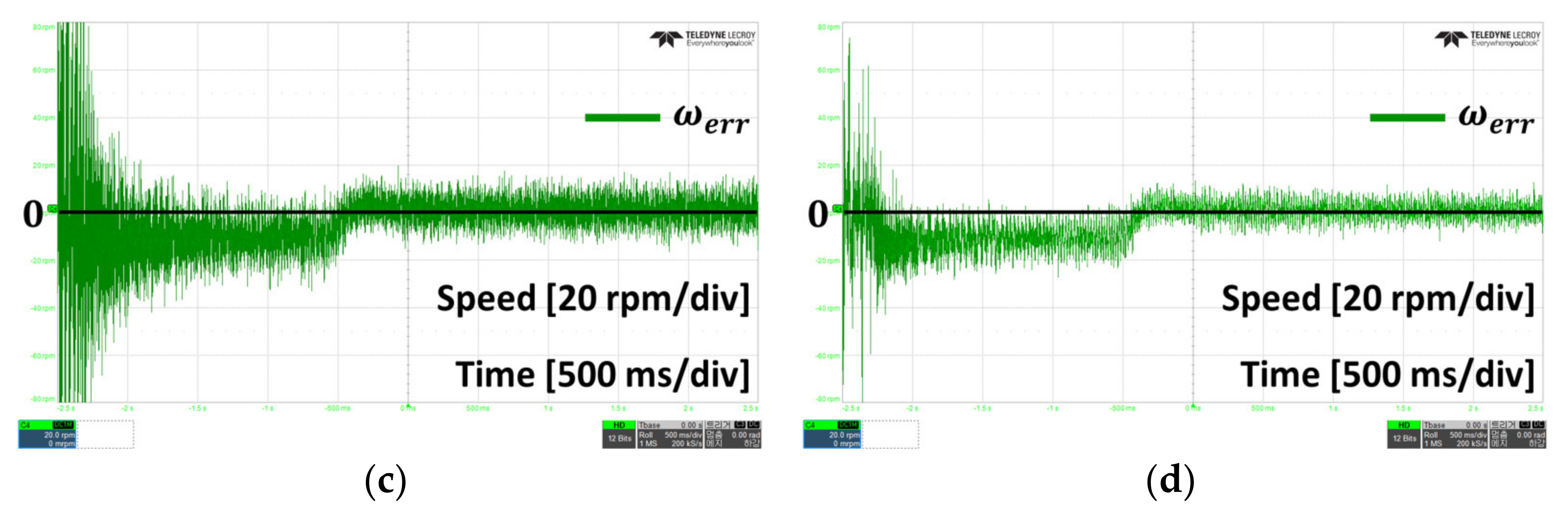
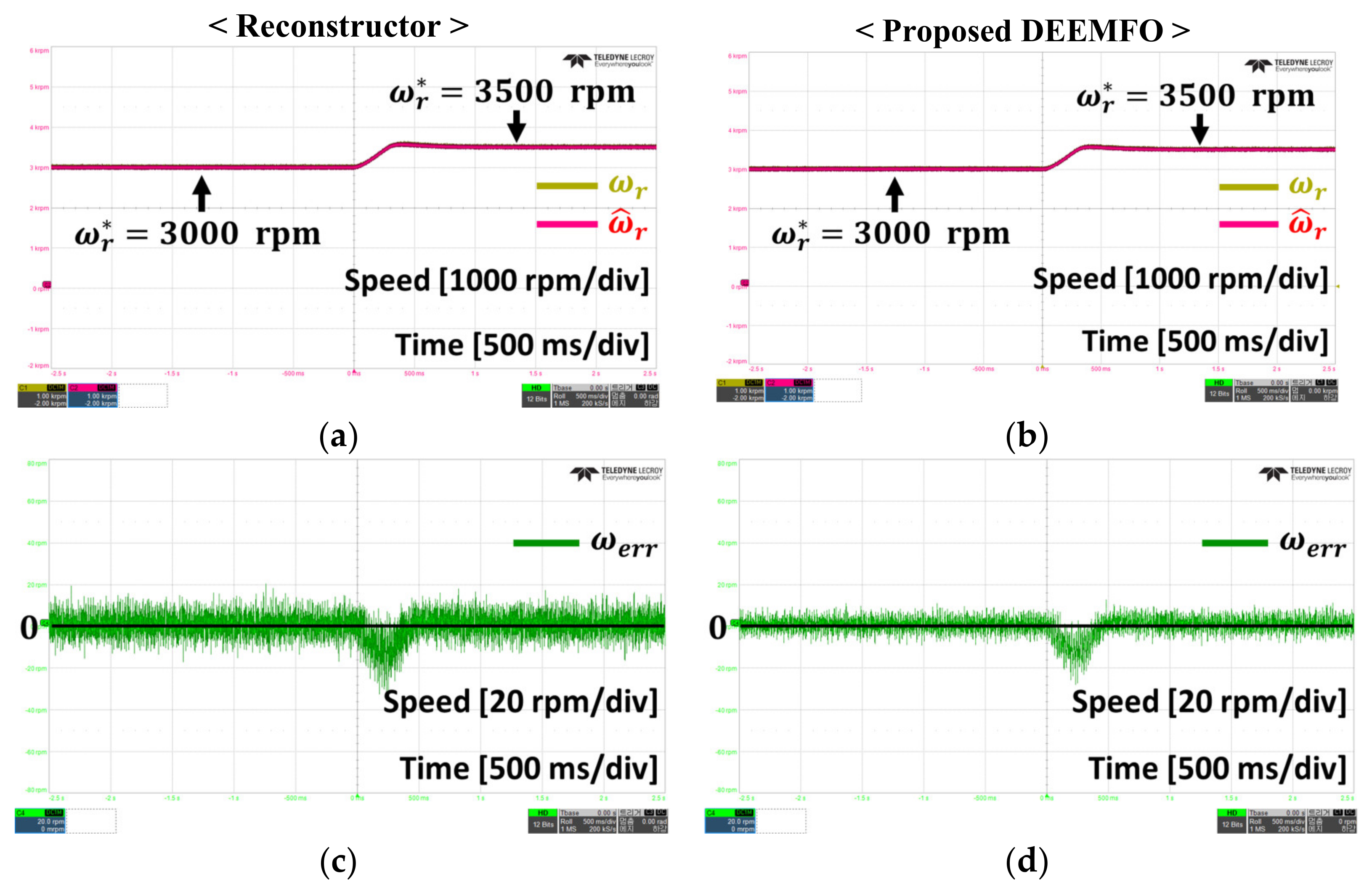
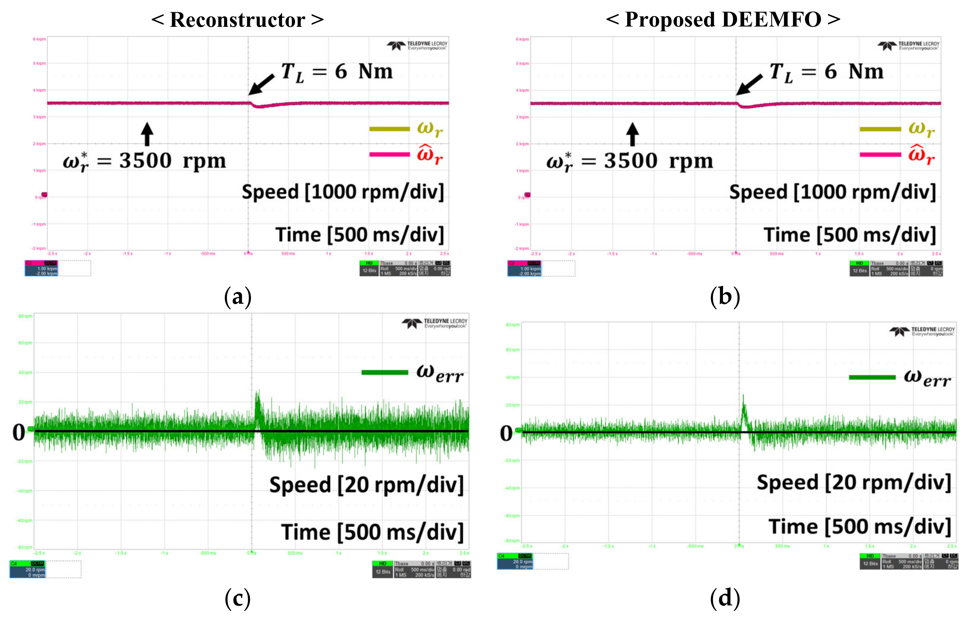
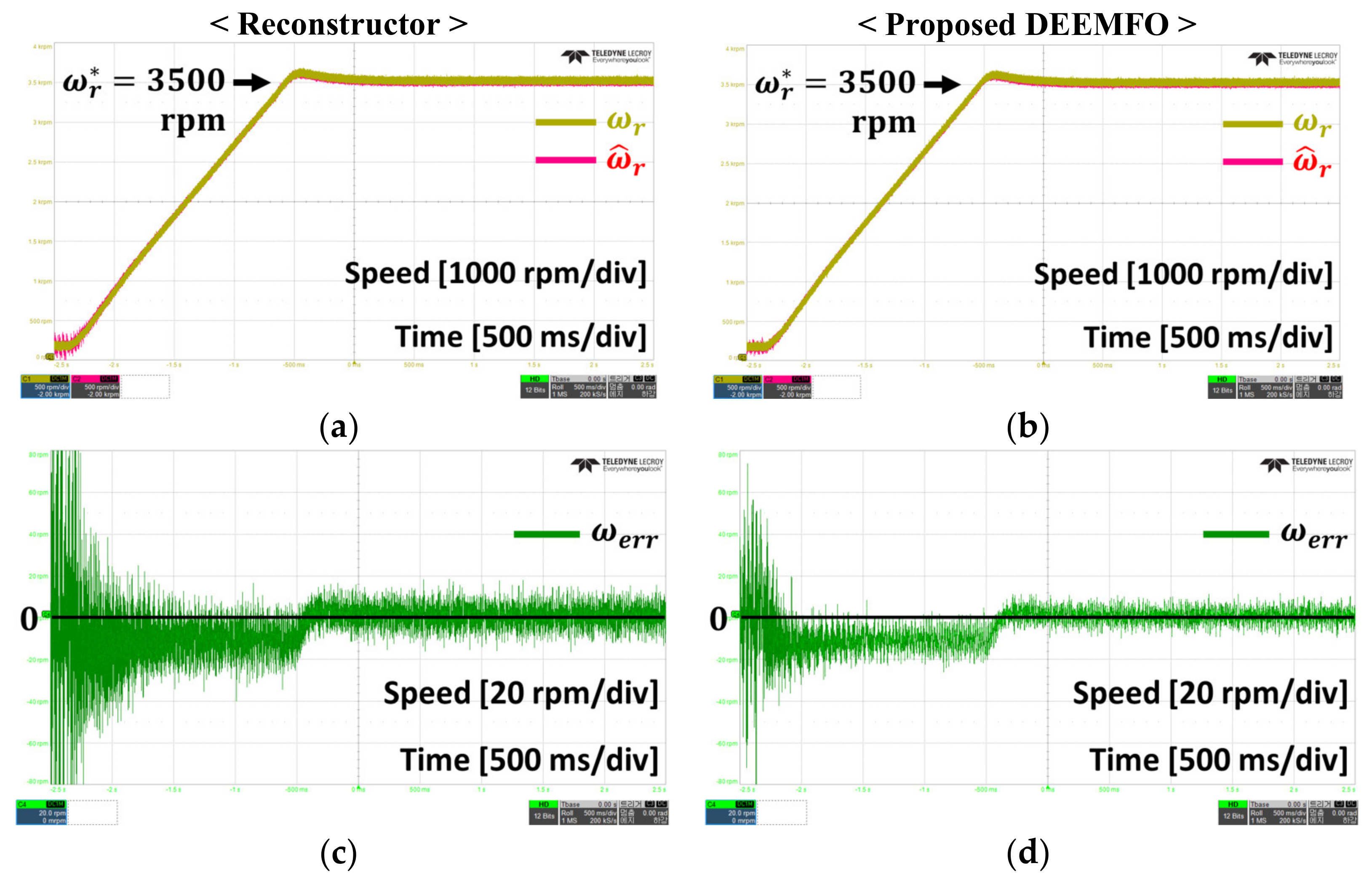
4.2. Experiment Result
5. Conclusions
Author Contributions
Funding
Conflicts of Interest
References
- Zhu, S.; Hu, Y.; Liu, C.; Jiang, B. Shaping of the Air Gap in a V-Typed IPMSM for Compressed-Air System Applications. IEEE Trans. Magn. 2021, 57, 8103705. [Google Scholar] [CrossRef]
- Yang, Y.; Sandra, M.C.; Rong, Y.; Berker, B.; Anand, S.; Hossein, D.; Ali, E. Design and Comparison of Interior Permanent Magnet Motor Topologies for Traction Applications. IEEE Trans. Transp. Electrif. 2017, 3, 86–97. [Google Scholar] [CrossRef]
- Lin, F.-J.; Hung, Y.-C.; Chen, J.-M.; Yeh, C.-M. Sensorless IPMSM drive system using saliency back-EMF-based intelligent torque observer with MTPA control. IEEE Trans. Ind. Inform. 2014, 10, 1226–1241. [Google Scholar]
- Wang, G.; Yang, R.; Xu, D. DSP-Based control of sensorless IPMSM drives for wide-speed-range operation. IEEE Trans. Ind. Electron. 2012, 60, 720–727. [Google Scholar] [CrossRef]
- Genduso, F.; Miceli, R.; Rando, C.; Galluzzo, G.R. Back EMF Sensorless-Control Algorithm for High-Dynamic Performance PMSM. IEEE Trans. Ind. Electron. 2010, 57, 2092–2100. [Google Scholar] [CrossRef]
- Mobarakeh, B.N.; Tabar, F.M.; Sargos, F.M. Mechanical sensorless control of PMSM with online estimation of stator resistance. IEEE Trans. Ind. Appl. 2004, 40, 457–471. [Google Scholar] [CrossRef]
- Sun, J.; Zhao, J.; Tian, L.; Song, Y.; Liu, Y. Bandwidth and Audible Noise Improvement of Sensorless IPMSM Drives based on Amplitude Modulation Multi-random Frequency Injection. IEEE Trans. Power Electron. 2022, 37, 14126–14140. [Google Scholar] [CrossRef]
- Pal, A.; Das, S.; Chattopadhyay, A.K. An Improved Rotor Flux Space Vector Based MRAS for Field-Oriented Control of Induction Motor Drives. IEEE Trans. Power Electron. 2018, 33, 5131–5141. [Google Scholar] [CrossRef]
- Yin, Z.; Li, G.; Zhang, Y.; Liu, J.; Sun, X.; Zhong, Y. A Speed and Flux Observer of Induction Motor Based on Extended Kalman Filter and Markov Chain. IEEE Trans. Power Electron. 2017, 32, 7096–7117. [Google Scholar] [CrossRef]
- Wang, G.; Li, Z.; Zhang, G.; Yu, Y.; Xu, D. Quadrature PLL-Based High-Order Sliding-Mode Observer for IPMSM Sensorless Control with Online MTPA Control Strategy. IEEE Trans. Energy Convers. 2013, 28, 214–224. [Google Scholar] [CrossRef]
- Zhang, G.; Wang, G.; Yuan, B.; Liu, R.; Xu, D. Active Disturbance Rejection Control Strategy for Signal Injection-Based Sensorless IPMSM Drives. IEEE Trans. Transp. Electrif. 2018, 4, 330–339. [Google Scholar] [CrossRef]
- Tang, Q.; Shen, A.; Luo, X.; Xu, J. IPMSM sensorless control by injecting bidirectional rotating HF carrier signals. IEEE Trans. Power Electron. 2018, 33, 10698–10707. [Google Scholar] [CrossRef]
- Kim, S.-Y.; Ha, I.J. A new observer design method for HF signal injection sensorless control of IPMSMs. IEEE Trans. Ind. Electron. 2008, 55, 2525–2529. [Google Scholar]
- Bolognani, S.; Oboe, R.; Zigliotto, M. Sensorless full-digital PMSM drive with EKF estimation of speed and rotor position. IEEE Trans. Ind. Electron. 1999, 46, 184–191. [Google Scholar] [CrossRef]
- Song, Z.; Yao, W.; Lee, K.; Li, W. An Efficient and Robust I-f Control of Sensorless IPMSM With Large Startup Torque Based on Current Vector Angle Controller. IEEE Trans. Power Electron. 2022, 37, 15308–15321. [Google Scholar] [CrossRef]
- Zhang, Y.; Yin, Z.; Bai, C.; Wang, G.; Liu, J. A Rotor Position and Speed Estimation Method Using an Improved Linear Extended State Observer for IPMSM Sensorless Drives. IEEE Trans. Power Electron. 2021, 36, 14062–14073. [Google Scholar] [CrossRef]
- Sun, X.; Zhang, Y.; Tian, X.; Cao, J.; Zhu, J. Speed Sensorless Control for IPMSMs Using a Modified MRAS With Gray Wolf Optimization Algorithm. IEEE Trans. Electrif. 2022, 8, 1326–1337. [Google Scholar] [CrossRef]
- Chen, Z.; Tomita, M.; Doki, S.; Okuma, S. An extended electromotive force model for sensorless control of interior permanent-magnet synchronous motors. IEEE Trans. Ind. Electron. 2003, 50, 288–295. [Google Scholar] [CrossRef]
- Morimoto, S.; Kawamoto, K.; Sanada, M.; Takeda, Y. Sensorless control strategy for salient-pole PMSM based on extended EMF in rotating reference frame. IEEE Trans. Ind. Appl. 2002, 38, 1054–1061. [Google Scholar] [CrossRef]
- Ko, J.S.; Lee, J.H.; Chung, S.K.; Youn, M.J. A robust digital position control of brushless DC motor with deadbeat load torque observer. IEEE Tran. Ind. Elec. 1993, 40, 512–520. [Google Scholar] [CrossRef]
- Bose, B.K. Modern Power Electronics and AC Drives; Prentice-Hall Inc.: Upper Saddle River, NJ, USA, 2002. [Google Scholar]
- Astrom, K.J.; Wittenmark, B. Computer-Controlled Systems: Theory and Design, 3rd ed.; Prentice Hall: Hoboken, NJ, USA, 1996. [Google Scholar]


| Parameter | Value | Unit |
|---|---|---|
| Rated power | 4.0 | kW |
| Rated speed | 3500 | r/min |
| Rated torque | 12 | Nm |
| Rated voltage | 380 | V |
| Rated Current | 10 | A |
| Stator resistance () | 0.332 | |
| Inductance d-axis () | 9.91 | |
| Inductance q-axis () | 10.93 | |
| Flux linkage | 0.118 | |
| Pole pairs | 5 | - |
| Parameter Variation | Reconstructor | DEEMFO |
|---|---|---|
| X | X | |
| X | O | |
| ⁝ | X | O |
| O | O | |
| ⁝ | O | O |
| O | O | |
| ⁝ | O | O |
| O | O | |
| O | O | |
| ⁝ | X | O |
| X | O | |
| X | X | |
| X | X | |
| X | O | |
| ⁝ | X | O |
Publisher’s Note: MDPI stays neutral with regard to jurisdictional claims in published maps and institutional affiliations. |
© 2022 by the authors. Licensee MDPI, Basel, Switzerland. This article is an open access article distributed under the terms and conditions of the Creative Commons Attribution (CC BY) license (https://creativecommons.org/licenses/by/4.0/).
Share and Cite
Kim, S.-T.; Yoon, I.-S.; Jung, S.-C.; Ko, J.-S. Robust Sensorless Control of Interior Permanent Magnet Synchronous Motor Using Deadbeat Extended Electromotive Force Observer. Energies 2022, 15, 7568. https://doi.org/10.3390/en15207568
Kim S-T, Yoon I-S, Jung S-C, Ko J-S. Robust Sensorless Control of Interior Permanent Magnet Synchronous Motor Using Deadbeat Extended Electromotive Force Observer. Energies. 2022; 15(20):7568. https://doi.org/10.3390/en15207568
Chicago/Turabian StyleKim, Seung-Taik, In-Sik Yoon, Sung-Chul Jung, and Jong-Sun Ko. 2022. "Robust Sensorless Control of Interior Permanent Magnet Synchronous Motor Using Deadbeat Extended Electromotive Force Observer" Energies 15, no. 20: 7568. https://doi.org/10.3390/en15207568