Modeling of Direct-Drive Permanent Magnet Synchronous Wind Power Generation System Considering the Power System Analysis in Multi-Timescales

Abstract

The dynamics of wind power generation cannot be neglected in the modern power system and could have a great impact on the system dynamics, even raising the risk of a blackout. Because of this, power system simulation has to include the model of wind power generation. However, due to the high order of the full model of the wind power generator, it is impossible to model them in detail in the use of the power system dynamic simulation considering the thousands of wind generators in the grid. In this context, a simplified model is normally used with the trade-off in lower accuracy. As a direct-drive permanent magnet synchronous wind power generation system (D-PMSG) would take up a certain occupation in the modern power system, a proper D-PMSG simplified model is needed in the power system simulation. For a different research purpose in a different timescale, a different complexity of the model can be used to maximize the accuracy, in the meantime speeding up the simulation. This paper proposes a set of simplified models of the direct-drive permanent magnet synchronous wind power generation system (D-PMSG) and classifies them according to the timescale of the dynamics and the use cases, i.e., faults (transient stability analysis), system contingencies (voltage and frequency stability analysis) and wind speed variations (energy transformation). The accuracy of the proposed simplified models is verified by comparing them with the detailed D-PMSG electromagnetic transient mode in Matlab/Simulink, and their use case of the power system simulation is validated based on the case study of the IEEE 39-bus system considering the above scenarios.

1. Introduction

In a transition of the power system migrating into higher renewables and higher power electronics, wind power generation has been gradually replacing the traditional thermal power plant and becoming one of the main power sources in the modern power system [1]. The direct-drive permanent magnet synchronous wind power generation system (D-PMSG) has progressed with a low failure rate, high reliability, and high efficiency so that its share of the market has continued to increase in recent years [2,3,4]. Due to the characteristics of the D-PMSG on renewables, e.g., stochastic generation, and the power electronics, e.g., low inertia and multi-time dynamics, the wide use of the D-PMSG has introduced new instability issues in the modern power system, i.e., the harmonics stability and converter-driven stability [5,6,7,8]. To understand the complex interaction between the modern power system and the D-PMSG, an accurate and efficient D-PMSG model is needed.

The D-PMSG consists of a wind turbine (WT), a permanent magnet synchronous generator (PMSG), a full power converter (FPC), and its control system (pitch angle [9,10], maximum power tracking (MPPT) [11,12], virtual inertia control [13,14,15], etc.), of which dynamics present a multi-timescale characteristic, including the electromagnetic transients, electromechanical transients, and mechanical transients ranging [16] from 1 ms to 100 s, and of which the model is nonlinear with a high order. In the power system simulation, the accuracy, computational speed, and system scale cannot be satisfied in the meantime [17]. Although the electromagnetic transient model (EMT) of the D-PMSG can easily capture all the dynamics, it cannot be used in the simulation of a large national grid due to the limitation on the computational burden and the solver [18]. A simplified D-PMSG model can suit the large-scale power system simulation, but as a trade-off would lose accuracy, especially on the small-timescale dynamics. Therefore, the art of the model simplification with good accuracy has attracted a lot of attention. For example, for the power system dynamic simulation, references [19,20,21,22] have developed a full model of the D-PMSG applicable to the electromagnetic transient (EMT) simulation of the system. References [23,24,25,26] show that during grid incidents, the main response of the D-PMSG is determined by the grid-side converter (GSC) with its control; thus, they suggest simplifying the machine-side converter (MSC) to be a controlled current source. With regard to the wind power participation in the system frequency regulation, reference [27] proposed an average model of D-PMSG, considering the virtual inertia control. Reference [28] simplifies the whole D-PMSG model to be a single inertial unit in the form of a swing equation. For the small-signal stability analysis of the D-PMSG, reference [29] linearizes the full-order model while reference [30] proves that the small-signal instability is mainly related to the GSC and thus the MSC can be assumed to be simplified as a constant DC voltage. For the optimal power flow analysis considering the wind farms in the grid, literature [31,32,33] builds a static D-PMSG model as a PQ node, with the active power from the wind turbine and reactive power from the constant power factor setup.

Based on the above literature review, although many D-PMSG models are available, they are either too detailed for system-level studies or too simple to capture short-term dynamics. Intermediate models can achieve a certain level of accuracy while reducing the computational burden. References [34,35] propose a set of smart transformer and storage models used for a different purpose of the power system studies, whose philosophy is that the complexity of the model depends on the timescale of the interested dynamics and the focus of the study. Based on this concept, this paper proposes a simplified approach to the D-PMSG and establishes a set of differential-algebraic equation (DAE) models for the D-PMSG applicable to power system stability analysis. The specific contributions of this paper are:

(i)

Identifying the dominated active controls in a serial of timescales by means of parameter sensitivity analysis.

(ii)

Proposing a set of D-PMSG simplified models with different complexity in line with the parameter sensitivity analysis for the different purpose of the power system dynamic analysis.

(iii)

Defining the use case of the D-PMSG simplified models for the transient stability, voltage stability, and frequency stability analysis, respectively.

The remainder of the paper is organized as follows. Section 2 introduces the detailed DAE model of the D-PMSG. Section 3 presents the proposed simplified D-PMSG models and classifies them according to their complexity, timescales, and parameter sensitivity. Section 4 defines the applications for the proposed D-PMSG models. Section 5 verifies the accuracy of the proposed models based on the IEEE benchmark 39 bus system. Finally, Section 6 draws relevant conclusions.

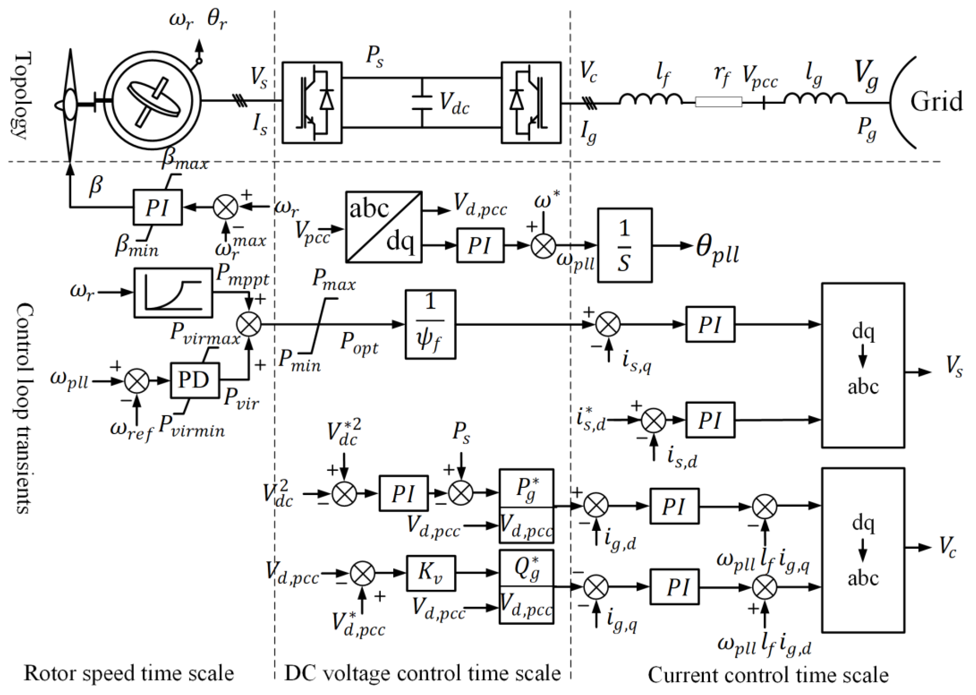
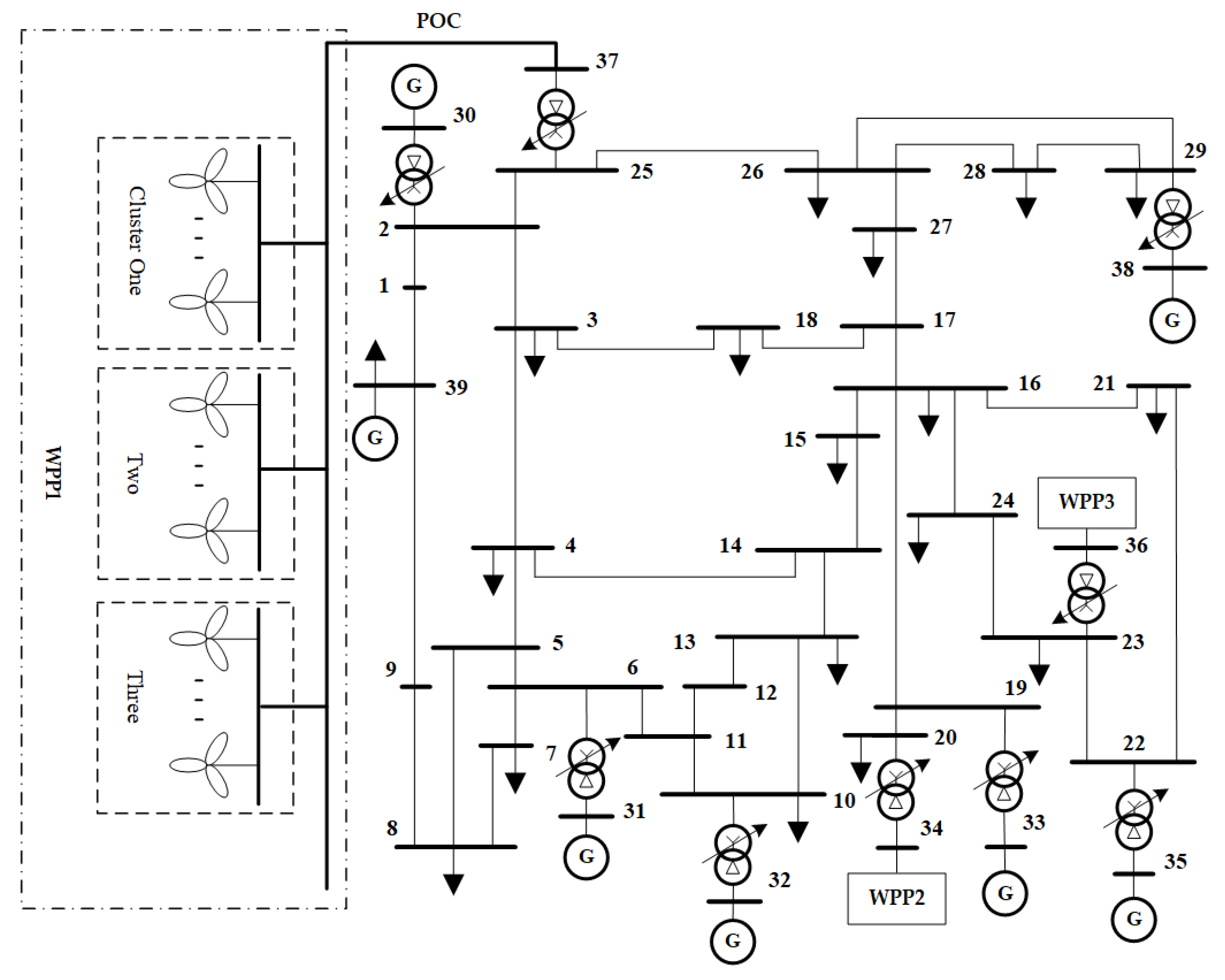
2. Modelling of the D-PMSG

Figure 1 shows the topology and control scheme of the D-PMSG, wherein the physical circuit, the WT, is connected directly to the PMSG via the drive shaft, and the generator is connected to the grid via the full power converter. In the control logic, pitch angle control is used to avoid over-speeding the turbine. The MSC is applied with MPPT and virtual inertia control to maximize the wind power generation and provide frequency support in the system. The GSC is applied phase-locked loop (PLL), DC voltage regulation, and reactive power control to achieve the grid synchronization, to maintain a fixed DC voltage and to provide the voltage support in the system. The meanings of the relevant variables in the D-PMSG are given in the notation section and are labeled in Figure 1.

2.1. Mechanical Model

The wind drives the turbine rotation, and the wind energy is transferred into kinetic energy and then into electrical energy; this process includes the conversion of the mechanical power in the turbine and the electromechanics in the PMSG.

The mechanical power is related to the wind speed and the turbine swept area as indicated below:

$$P_w=\frac{1}{2}{A}_r{\rho C}_p\left(\lambda ,\beta \right){v_w}^3$$

(1)

where $\lambda$ is the tip speed ratio, which can be expressed as:

$$\lambda =\frac{{\omega }_{r}R}{v_w}$$

(2)

$C_p\left(\lambda ,\beta \right)$ is the performance coefficient, which can be approximated as:

$$C_p\left(\lambda ,\beta \right)=0.5176\left(\frac{116}{{\lambda }_1}-0.4\beta -5\right)e^{-\frac{21}{{\lambda }_1}}+0.0068\lambda$$

(3)

And ${\lambda }_1$ is the coefficient, which normally can be set as:

$$\frac{1}{{\lambda }_1}=\frac{1}{\lambda +0.08\beta }-\frac{0.035}{{\beta }^3+1}$$

(4)

The D-PMSG converts mechanical energy into electrical energy, of which electromechanical dynamics of such power delivery are usually expressed as:

$$H{\stackrel{.}{\omega }}_r=T_w-T_e-D{\omega }_r$$

(5)

In the synchronous dq frame, the voltage of the PMSG stator is:

$$\{\begin{array}{c}{L}_{s,d}{\stackrel{.}{I}}_{s,d}=r_s{I}_{s,d}-{\omega }_r{L}_{s,q}{I}_{s,q}-V_{s,d}\\ L_{s,q}{\stackrel{.}{I}}_{s,q}=r_s{I}_{s,q}+{\omega }_r(L_{s,d}{I}_{s,d}+{\psi }_p)-V_{s,q}\end{array}$$

(6)

where the voltage of the PMSG stator is formed by the MSC

The PMSG electromagnetic torque is:

$$T_e=\left[{\psi }_p+\left({\omega }_r{L}_{s,d}-{\omega }_r{L}_{s,q}\right)I_{s,d}\right]I_{s,q}$$

(7)

The output power of the generator is:

$$\{\begin{array}{c}{P}_s=V_{s,d}{I}_{s,d}+V_{s,q}{I}_{s,q}\\ Q_s=V_{s,q}{I}_{s,d}-V_{s,d}{I}_{s,q}\end{array}$$

(8)

2.2. Full Power Converter Model

The FPC transmits the electrical power generated by the PMSG to the grid, which consists of the MSC, the DC bus, and the GSC.

The MSC and GSC are connected commonly at the DC bus. In the steady state, the power feeding into the DC capacitor from the MSC should be equivalent to the power flowing into the GSC. In transients, the unbalanced power between the input and output of the DC capacitor would be compensated by the capacitor itself, whose dynamics can be represented as follows:

$$\frac{1}{2}{C}_{dc}{\stackrel{.}{V}}_{dc}^2=-P_s-(V_{pcc,d}{I}_{g,d}+V_{pcc,q}{I}_{g,q})$$

(9)

The main function of the GSC in one respect is to achieve the synchronization at the PCC. In another respect, it provides stable DC voltage through active power regulation and an auxiliary service for voltage support through reactive power regulation.

The active exchange of the PCC with the grid is:

$$\{\begin{array}{c}{P}_g=V_g\cos \left({\delta }_g-{\delta }_{pll}\right)I_{g,d}+V_g\cos \left({\delta }_g-{\delta }_{pll}\right)I_{g,q}\\ Q_g=V_g\sin \left({\delta }_g-{\delta }_{pll}\right)I_{g,q}-V_g\sin \left({\delta }_g-{\delta }_{pll}\right)I_{g,d}\\ V_{pcc,d}=V_g\cos \left({\delta }_g-{\delta }_{pll}\right)-{\omega }_g{L}_g{I}_{g,q}\\ V_{pcc,q}=V_g\cos \left({\delta }_g-{\delta }_{pll}\right)+{\omega }_g{L}_g{I}_{g,d}\end{array}$$

(10)

The GSC synchronization process at the PCC is achieved with a PLL, of which the steady state is the q-axis voltage stabilizing at zero.

$$\{\begin{array}{c}\Delta {\omega }_{pll}=K_{pll.p}{V}_{q,pcc}+K_{pll,i}{\mu }_{pll}\\ {\stackrel{.}{\mu }}_{pll}=V_{pcc,q}\\ {\omega }_{pll}={\omega }^{*}+\Delta {\omega }_{pll}\\ {\stackrel{.}{\delta }}_{pll}={\omega }_{pll}\end{array}$$

(11)

In addition, the GSC is equipped with a filter to eliminate the harmonics, whose dynamics can be represented as follows.

$$\{\begin{array}{c}{L}_f{\stackrel{.}{I}}_{g,d}=V_{pcc,d}-V_{c,d}-{\omega }_{pll}{L}_f{I}_{g,q}-r_f{I}_{g,d}\\ L_f{\stackrel{.}{I}}_{g,q}=V_{pcc,q}-V_{c,q}-{\omega }_{pll}{L}_f{I}_{g,d}-r_f{I}_{g,q}\end{array}$$

(12)

2.3. Control System Model

The control of the D-PMSG aims to maximize the power generation and stably connect to the grid including the pitch angle control, maximum power control, virtual inertia control, MSC control, and GSC control.

The main function of the pitch angle control system is to restrict the WT speed at ${\omega }_{max}$ by means of the PI controller. A servo system is used to adjust the pitch movement within the range of $\left[{\beta }_{min}{,\beta }_{ max}\right]$, where the pitch movement can be represented as a first order delay process with the time constant $T_{\beta }$.

$$\frac{d\beta }{dt}=\frac{1}{T_{\beta }}{(\beta }_{ref}-\beta )$$

(13)

$${\beta }_{ref}=\{\begin{array}{cc}\hfill {\beta }_{max},& {\beta }_0{>\beta }_{max}\hfill \\ \hfill {\beta }_0,& {\beta }_{min}{<\beta }_0{<\beta }_{max}\hfill \\ \hfill {\beta }_{min},& {\beta }_0{<\beta }_{min}\hfill \end{array}$$

(14)

where ${\beta }_0$ is the pitch movement set point:

$$\{\begin{array}{c}{\beta }_0=K_{mp,p}({\omega }_r-{\omega }_{max})+K_{mp,i}\sigma \\ \sigma ={\omega }_r-{\omega }_{max}\end{array}$$

(15)

From Equation (2), it can be seen that the pitch angle $\beta$ is constant, and when the wind speed changes, by controlling the speed of the WT it can achieve the optimal blade tip speed ratio ${\lambda }_{opt}$, which makes WT track the maximum power point, which can be expressed as:

$$P_{mppt}=K_{mppt}{\omega }_r^3$$

(16)

where: $K_{mppt}=0{.5\pi \rho C}_{pmax}{R}^5{\omega }_r^3{/\lambda }_{opt}^3$.

In order to provide the auxiliary service on frequency support, the virtual inertia control based on the proportional–differential (PD) control is added on the MPPT control. When the grid frequency varies, the frequency regulation auxiliary power provided by the turbine is:

$$P_{vir}=\{\begin{array}{cc}\hfill P_{virmax},& P_0{>P}_{virmax}\hfill \\ \hfill P_0,& P_{min}{<P}_0{<P}_{virmax}\hfill \\ \hfill P_{virmin},& P_0{<P}_{virmin}\hfill \end{array}$$

(17)

where $P_0$ is the power set point from the virtual inertia control:

$$P_0=K_p({\omega }_{pll}-{\omega }^{*})K_d{\stackrel{.}{\omega }}_{pll}$$

(18)

For the safe operation of the D-PMSG, the output power must be limited as follows:

$$P_{ref}=\{\begin{array}{c}{P}_{max}{,P}_{mppt}{+P}_{vir}{>P}_{max}\\ P_{mppt}{+P}_{vir}{,P}_{min}{<P}_{mppt}{+P}_{vir}{<P}_{max}\\ P_{min}{,P}_{mppt}{+P}_{vir}{<P}_{min}\end{array}$$

(19)

Therefore, the reference torque output by the WT is:

$$T_{ref}=\frac{P_{ref}}{{\omega }_r}$$

(20)

The D-PMSG tracks the reference torque through the MSC. Here, the MSC uses zero d-axis stator current control [36], the basic principle of which is to use the q-axis current to control the electric field of the PMSG orthogonal to the magnetic field of the permanent magnet to obtain the maximum torque; the d-axis current is generally set to be null in order to minimize generator losses. Thus, the MSC control system model can be expressed as:

$$\{\begin{array}{c}{I}_{s,d}^{*}=0\\ I_{s,q}^{*}=-\frac{T_{ref}}{{\psi }_p}\end{array}$$

(21)

The actual current of the MSC is then controlled by the current inner loop to track the reference current command:

$$\{\begin{array}{c}{V}_{s,d}=K_{mc,p}(I_{s,d}^{*}-I_{s,d})+K_{mc,i}{\epsilon }_d-{\omega }_s{L}_q{I}_{s,q}\\ V_{s,q}=K_{mc,p}(I_{s,q}^{*}-I_{s,q})+K_{mc,i}{\epsilon }_q+{\omega }_s(L_d{I}_{s,d}+{\psi }_p)\\ {\stackrel{.}{\epsilon }}_d=I_{s,d}^{*}-I_{s,d}\\ {\stackrel{.}{\epsilon }}_q=I_{s,q}^{*}-I_{s,q}\end{array}$$

(22)

The control objective of the GSC aims to provide constant DC voltage and grid-side reactive voltage support, where the DC voltage control can be described as:

$$\{\begin{array}{c}{P}_g^{*}=P_s-\left[K_{gv,p}\right(V_{dc}^{*2}-V_{dc}^2)+K_{gv,i}{\gamma }_{dc}]\\ {\stackrel{.}{\gamma }}_{dc}=V_{dc}^{*2}-V_{dc}^2\end{array}$$

(23)

While the reactive power reference is set via the voltage support:

$$Q_g^{*}=K_v\left(V_{pcc,d}^{*}-V_{pcc,d}\right)$$

(24)

From the above power references, we can obtain current reference commands:

$$\{\begin{array}{c}{I}_{g,d}^{*}=P_g^{*}/V_{pcc,d}\\ I_{g,q}^{*}=-Q_g^{*}/V_{pcc,q}\end{array}$$

(25)

Again, the current inner loop control of the controller can be expressed as:

$$\{\begin{array}{c}{V}_{c,d}=K_{gc,p}(I_{g,d}^{*}-I_{g,d})+K_{gc,i}{ϵ}_d-{\omega }_{pll}{L}_f{I}_{g,q}\\ V_{c,q}=K_{gc,p}(I_{g,q}^{*}-I_{g,q})+K_{gc,i}{ϵ}_q+{\omega }_{pll}{L}_f{I}_{g,d}\\ {\stackrel{.}{ϵ}}_d=I_{g,d}^{*}-I_{g,d}\\ {\stackrel{.}{ϵ}}_q=I_{g,q}^{*}-I_{g,q}\end{array}$$

(26)

Equations (1)–(26) represent the full-order differential-algebraic equation (DAE) model of the D-PMSG.

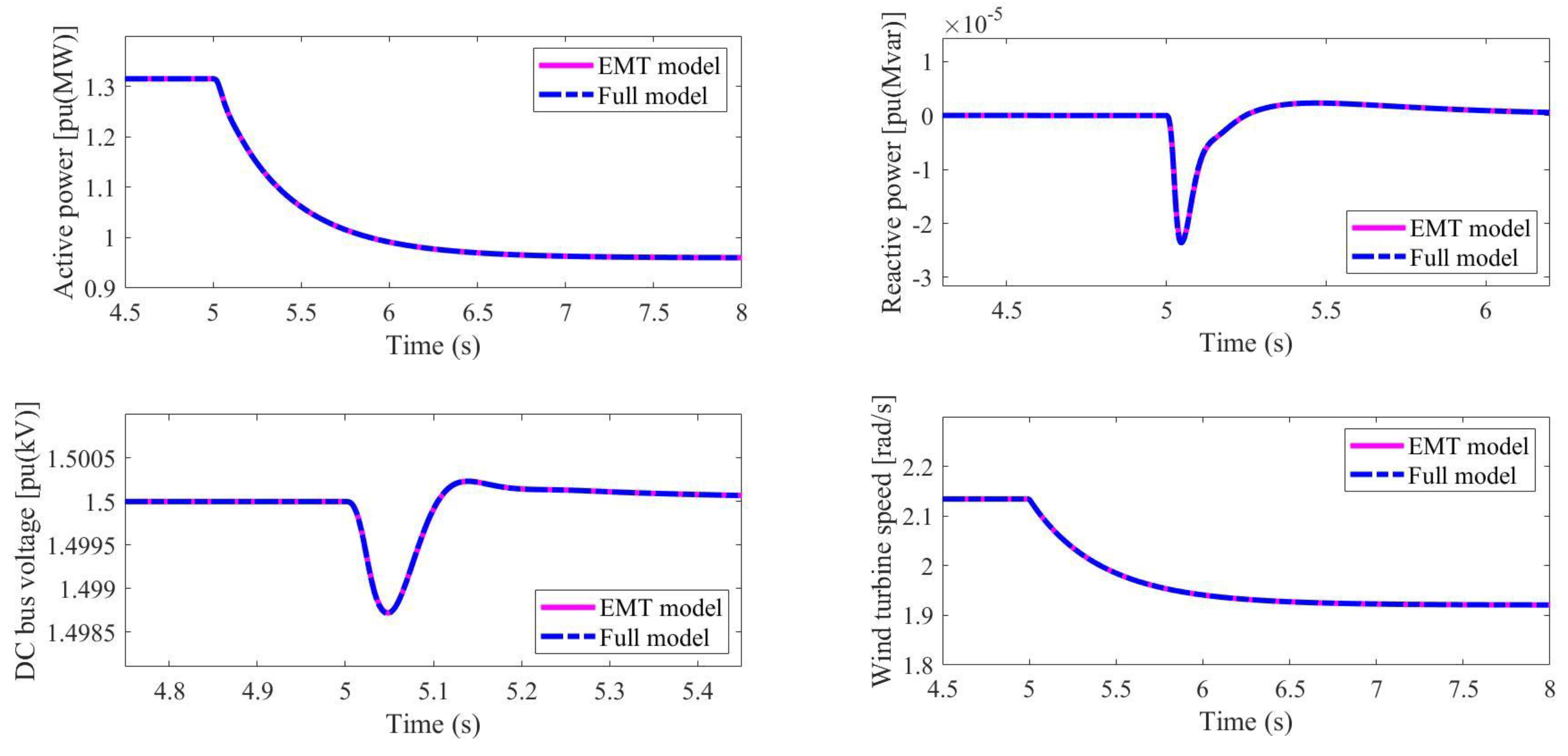
2.4. Model Validation via Simulation

Since latterly the simplified models have been derived from the full-order DAE model, the accuracy of the full-order DAE model is crucial. In order to verify its accuracy, we built a D-PMSG EMT model and a full-order DAE model based on Matlab/Simulink. The full-order DAE model built here uses only the mathematical module. The test system is a 1.5 MW/690 V D-PMSG connecting to a grid via a 5 mH grid impedance, where the main parameters are given in

Table 1. D-PMSG parameters and settings.

Parameter	Value
$S_n$	1 MW
$V_n$	1 kV
$R$	38 m
$V_w$	10 m/s
$\rho$	1.225 kg/m3
$H$	0.5 s
$P$	48
${\psi }_p$	1.885 pu
$r_s{/L}_s$	3.5 × 10−3 pu/5.44 × 10−2 pu
$L_g{/r}_f{/L}_f$	9.07 × 10−3 pu/5.77 × 10−5 pu/9.07 × 10−2 pu
$C_{dc}$	1.04 × 10−4 pu
$V_{dc}$	1.5 pu
$V_g$	0.69 pu
$K_p/K_d/K_v$	3.1416/0.5236/0

.

Figure 2 shows comparison results of the D-PMSG full model with its electromagnetic transient (EMT) model at the grid side, DC bus, and machine side in the case of the grid voltage drop from 1 pu to 0.9 pu at 5 s. Figure 3 shows the results of the grid frequency drop at 5 s from 50 Hz to 49 Hz with a 0.5 Hz/s ramp. Figure 4 shows the results of the wind speed stepdown from 10 m/s to 9 m/s at 5 s.

As shown in Figure 2, Figure 3 and Figure 4, the full-order DAE model can well capture the D-PMSG dynamics in a multi-timescale, including the transient, frequency and voltage responses.

3. Approximated D-PMSG Models

The full-order DAE model of the D-PMSG involves multiple responses at different times in a power system. Accurate modeling of transients on shorter timescales would lead to a dramatic increase in the computational burden, especially in the large-scale power system that simulates several D-PMSG stations. For the purpose of a lower computational burden, a simplified model is necessary.

Figure 5 shows the response timescale of the power system dynamics and that of the D-PMSG control dynamics. According to the timescale of the research focus, the small-timescale dynamics can be assumed to have worked while the large-timescale dynamics can be assumed to have not been activated. For example, for the research interest in the grid fault, the MSC and GSC dynamics have to be precisely modeled while the pitch angle control could be set to be unvaried. For the research interest in the inertia response, the current and voltage controller transients of the MSC and GSC can be ignored. For the research interest in the primary response, only the turbine regulation needs to be modeled in detail.

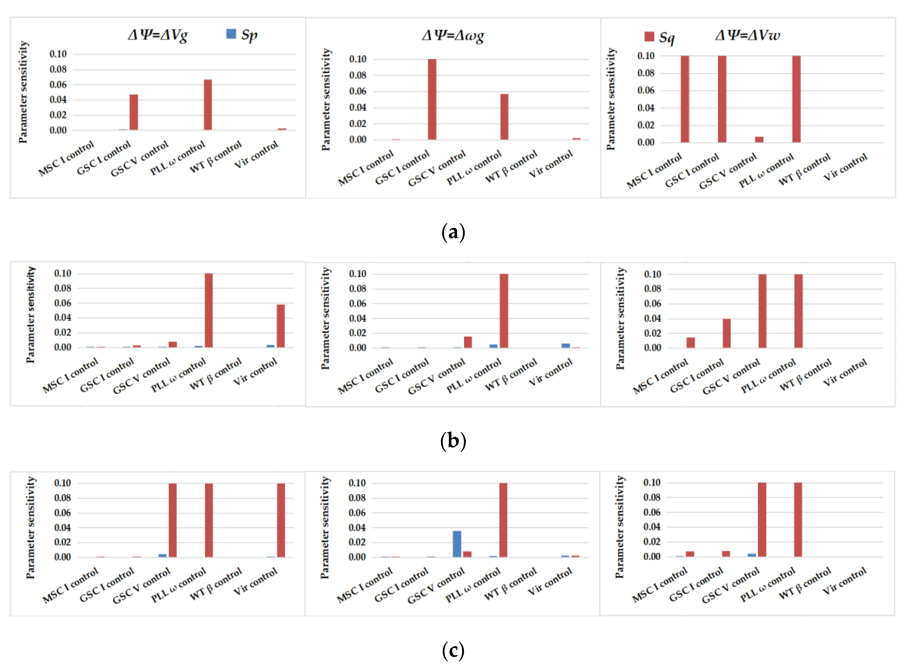
3.1. Parameter Sensitivity

Parameter sensitivity is a method that can be used to evaluate the dependence of the interested dynamics on the parameters. Since the D-PMSG model built in this paper aims to fit into power system simulation, the D-PMSG responses, i.e., active and reactive power injection, at the PCC would be of importance. Thus, here we analyze the parameter sensitivity of the power injection from the D-PMSG to the grid:

$$S_p=\left|\frac{\Delta P}{\Delta \Psi }\right|=\left|\frac{P_{\Psi ,t}-P_{0,t}}{0{.1P}_{0,t}}\right|$$

(27)

$$S_q=\left|\frac{\Delta Q}{\Delta \Psi }\right|=\left|\frac{Q_{\Psi ,t}-Q_{0,t}}{0{.1Q}_{0,t}}\right|$$

(28)

where $\Psi$ represents the parameter of interest, $P_{0,t}$, $Q_{0,t}$ are the grid power exchange from the D-PMSG at the timescale t using the original parameters, $P_{\Psi ,t}$, $Q_{\Psi ,t}$ are the powers at the same timescale but with the parameter Ψ increased by 10%.

Based on Matlab/Simulink simulation experiments, the parameter sensitivity in different scenarios and in different timescales can be obtained. Figure 6 shows the results of the D-PMSG parameter sensitivity at the timescale of 1 ms, 10 ms and 100 ms in the scenarios of the grid voltage drops to 0.5 pu (graph on the left), the grid frequency drops to 49.5 Hz (graph in the middle) and the wind speed step changes from 10 m/s to 9 m/s (graph on the right). As expected, in the 1 ms timescale the system transients are dominated by current controller transients, so the electromagnetic part of the system must be accurately modeled, while the pitch angle controller transients have not been activated; In the 10 ms timescale, the system voltage controller transients gradually increase while the current controller transients become less important; In the 100 ms timescale, the electrical part of the system transient is completed, and the virtual inertia control transient becomes dominated. Based on the above parameter sensitivity analysis, the model of the D-PMSG can be simplified in a line with the interested timescales, i.e., 10 ms and 100 ms, as follows.

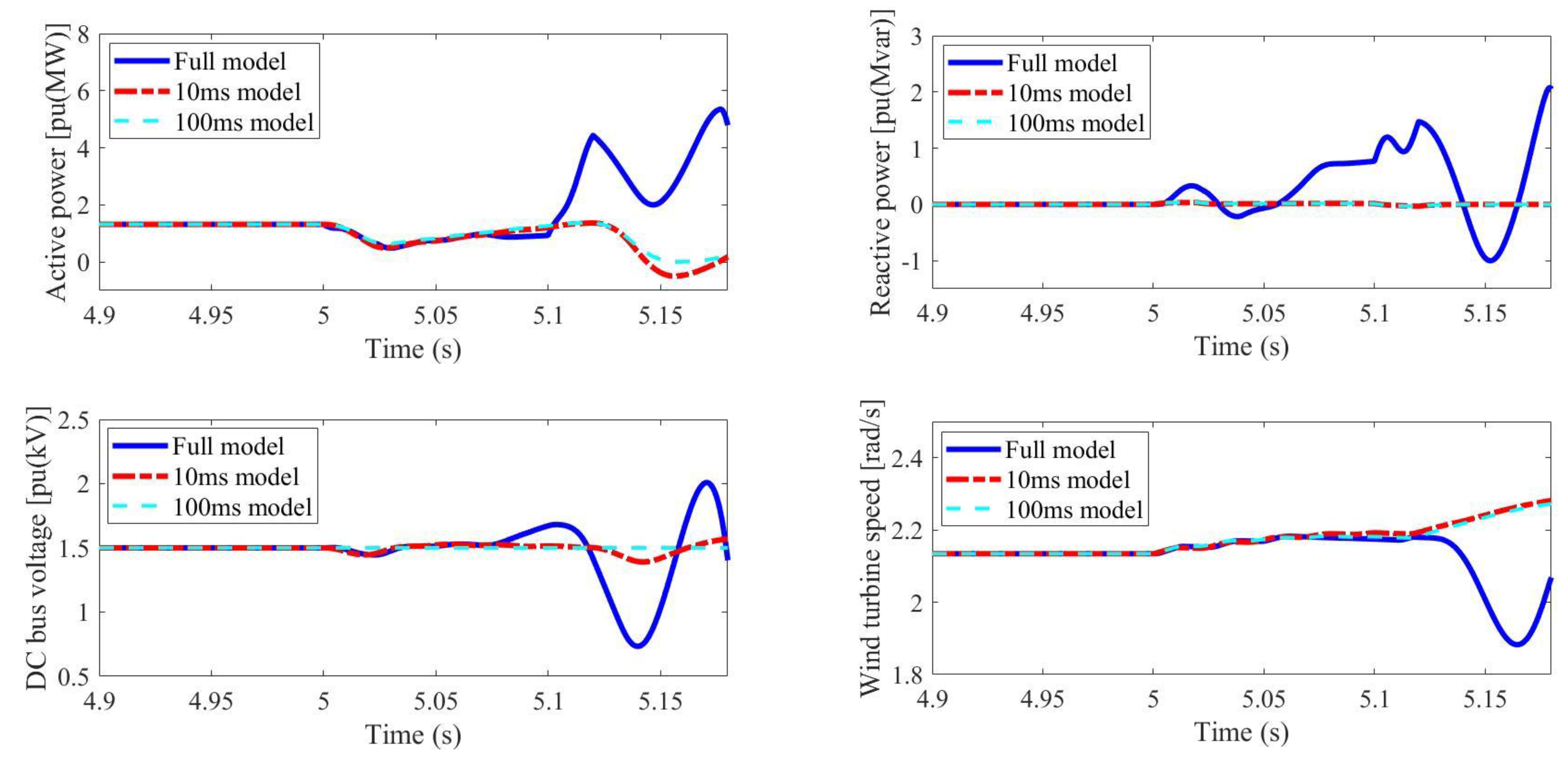
3.2. 10 ms Model

When the interested timescale is 10 ms, the fast frequency response including the transient of the FPC current controller and line filter can be ignored. Thus, the relevant transients in the format of the differential equation can be turned into the format of the algebraic equation that (6)–(8) in the mechanical stage, (9), (10) and (12) in the FPC stage and (22) and (26) in the control system stage can be simplified as follows:

$$T_e=\left[{\psi }_p+\left({\omega }_r{L}_{s,d}-{\omega }_r{L}_{s,q}\right)i_{s,d}^{*}\right]i_{s,q}^{*}$$

(29)

$$P_s=T_e{\omega }_r-r_s{(i}_{s,d}^{*2}+i_{s,q}^{*2})$$

(30)

$$\{\begin{array}{c}{P}_g=V_g\cos \left({\delta }_g-{\delta }_{pll}\right)I_{g,d}^{*}+V_g\cos \left({\delta }_g-{\delta }_{pll}\right)I_{g,q}^{*}\\ Q_g=V_g\sin \left({\delta }_g-{\delta }_{pll}\right)I_{g,q}^{*}-V_g\sin \left({\delta }_g-{\delta }_{pll}\right)I_{g,d}^{*}\\ V_{pcc,d}=V_g\cos \left({\delta }_g-{\delta }_{pll}\right)-{\omega }_g{L}_g{I}_{g,q}^{*}\\ V_{pcc,q}=V_g\cos \left({\delta }_g-{\delta }_{pll}\right)+{\omega }_g{L}_g{I}_{g,d}^{*}\end{array}$$

(31)

$$\frac{1}{2}{C}_{dc}\dot{V_{dc}^2}=-P_s-\left(V_{pcc,d}{I}_{g,d}^{*}+V_{pcc,q}{I}_{g,q}^{*}\right)$$

(32)

3.3. 100 ms Model

When the interested research on the primary frequency response is at a timescale of 100 ms, the dynamics of the controller related to the FPC can be ignored. Based on the above 10 ms model, additionally, (11) in the FPC stage and (23) in the control system stage can be simplified as follows.

$${\omega }_{pll}={\omega }_g$$

(33)

$$V_{dc}=V_{dc}^{*}$$

(34)

3.4. Summary

For simplicity, we name the model for 10 ms -order and 100 ms -order timescale research the “10 ms model” and “100 ms model”, respectively.

Table 2. Summary of the D-PMSG models.

D-PMSG Stage	Full Model	10 ms Model	100 ms Model
Mechanical model	(1–8)	(1–5) (29–30)	(1–5) (29–30)
FPC model	(9–12)	(11) (31–32)	(31–33)
Control system model	(13–26)	(13–21) (23–25)	(13–21) (24–25) (34)
Time step	0.1 ms	1 ms	10 ms

summarizes the simplified D-PMSG models, where computational time step in the power system simulation is set to be at least 1/10 of the minimum time constant of the control dynamics in that model.

4. Use Cases

This section defines the use case of the D-PMSG models in the scenarios of the system faults, grid frequency change, and wind speed variations. Since the purpose is to verify the accuracy and applicability of the D-PMSG model itself, a single machine connecting to the infinite bus is used here and built in Matlab/Simulink. The parameters are detailed in Table 1. Initially, the grid frequency is at 50 Hz and the grid voltage is 1 pu.

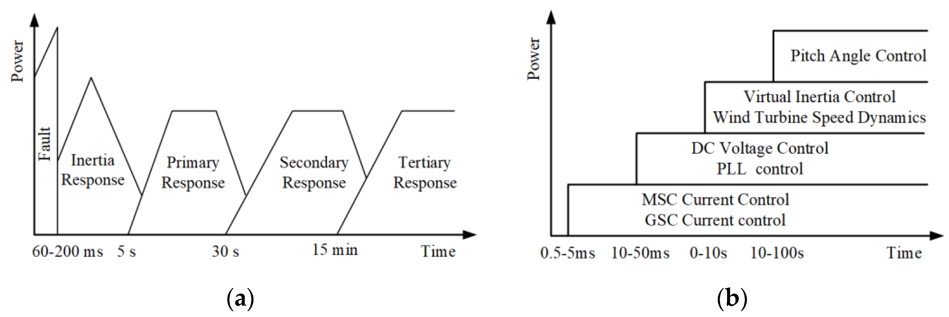
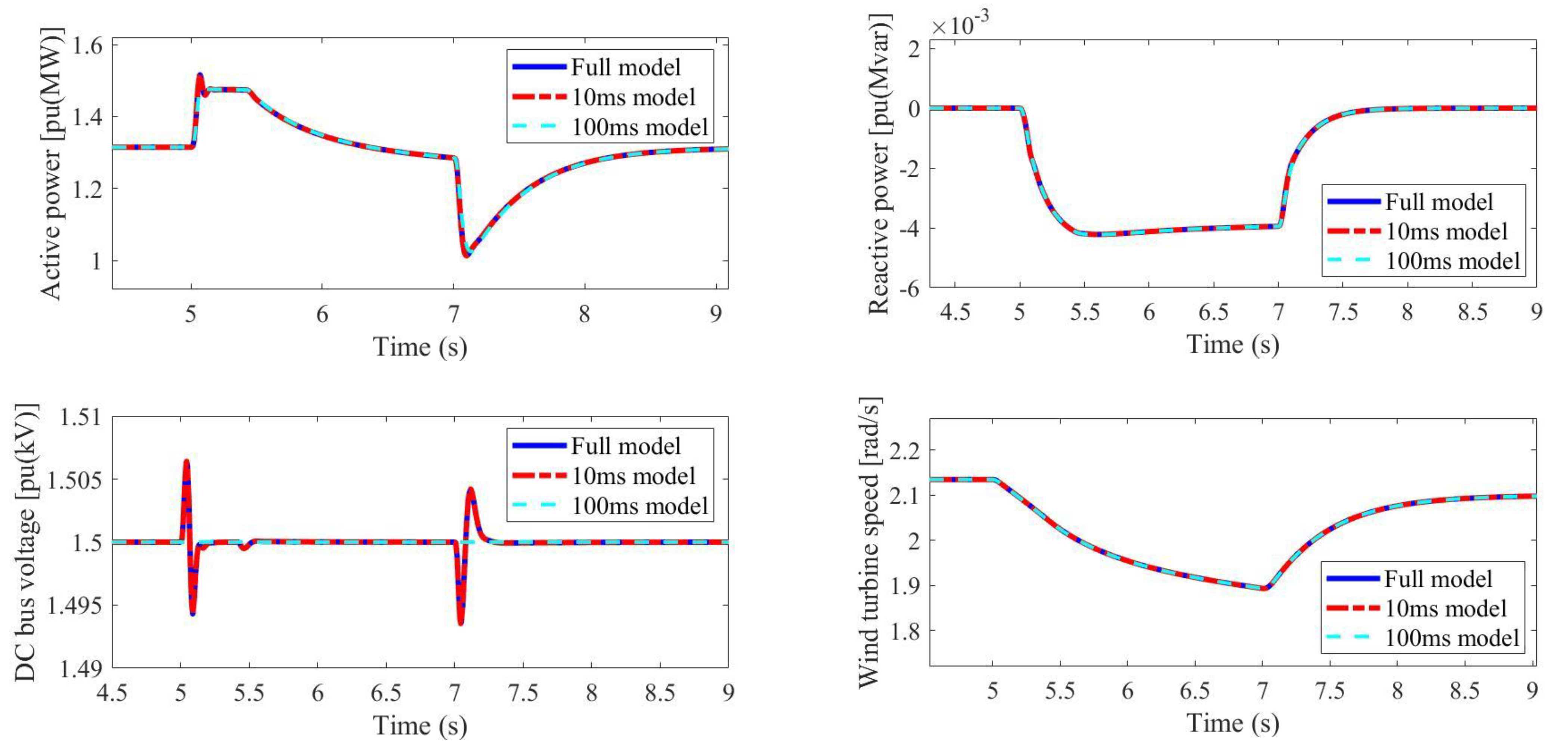
4.1. Fault Response

According to grid regulations, faults should be cleared within 50 ms to 100 ms and, meanwhile, the D-PMSG has to keep connecting with the grid. The model should precisely reflect the D-PMSG dynamics during the process of the fault ride through. The grid voltage drops to 0.2 pu at 5 s and then recovers to 1 pu at 5.1 s. Figure 7 shows the comparative results using different D-PMSG models at the AC port, DC port, and turbine port.

From Figure 7, it can be seen that the D-PMSG full model presents a loss of synchronization after the fault occurrence, while the simplified models still show a stable response. This is because the simplified model renders the D-PMSG as a constant current source, which neglects the current transients. This transient can enlarge the power imbalance between the MSC and GSC and then result in instability, which can be captured only by the full model. Hence, in the scenario of the grid fault, the full model must be used.

4.2. Frequency Event

The grid code now requires that all the renewable generations have an ability on the frequency support. In this scenario, the grid frequency decreases from 50 Hz to 49 Hz at a rate of 0.5 Hz/s at 5 s, and Figure 8 shows the comparative results using different D-PMSG models at the AC port, DC port, and turbine port.

From Figure 8, it can be seen that the 10 ms model can precisely capture the D-PMSG dynamics at all the ports as the full model does. Since the 100 ms model neglects the DC voltage control dynamics, it cannot reflect the DC bus voltage dynamics during this process, but this will not affect its accuracy on the modelling of the turbine and grid dynamic interactions. Hence, the 10 ms model is enough to be used to represent complete D-PMSG dynamics in the scenario of the frequency event. In addition, if the DC voltage is not of interest and the grid interaction is of interest, then the 100 ms model is applicable as well.

4.3. Wind Speed Event

The basic function of the D-PMSG is to convert wind energy into electrical energy. A D-PMSG model is needed in order to analyze the effect of renewable stochastics on the grid frequency and voltage variance. The wind speed changes from 10 m/s to 9 m/s at 5 s and Figure 9 shows the comparative results.

The usage of the model in this scenario is very similar to the scenario of the frequency event that the 10 ms model is the most suitable and the 100 ms model may be possible.

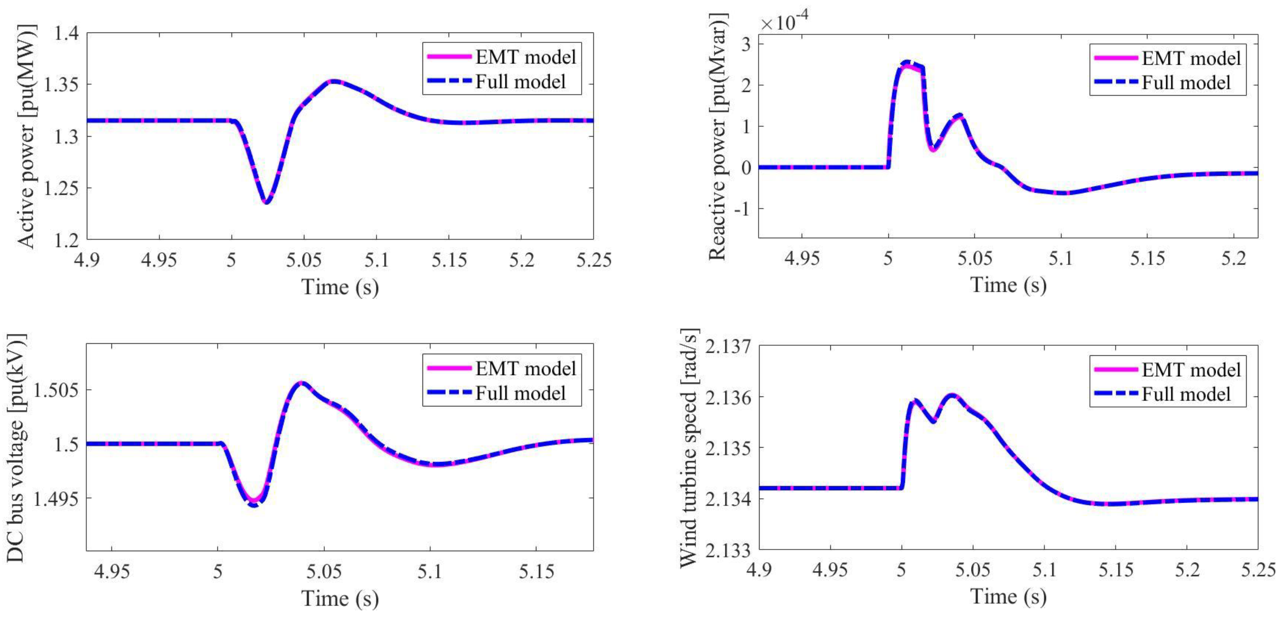
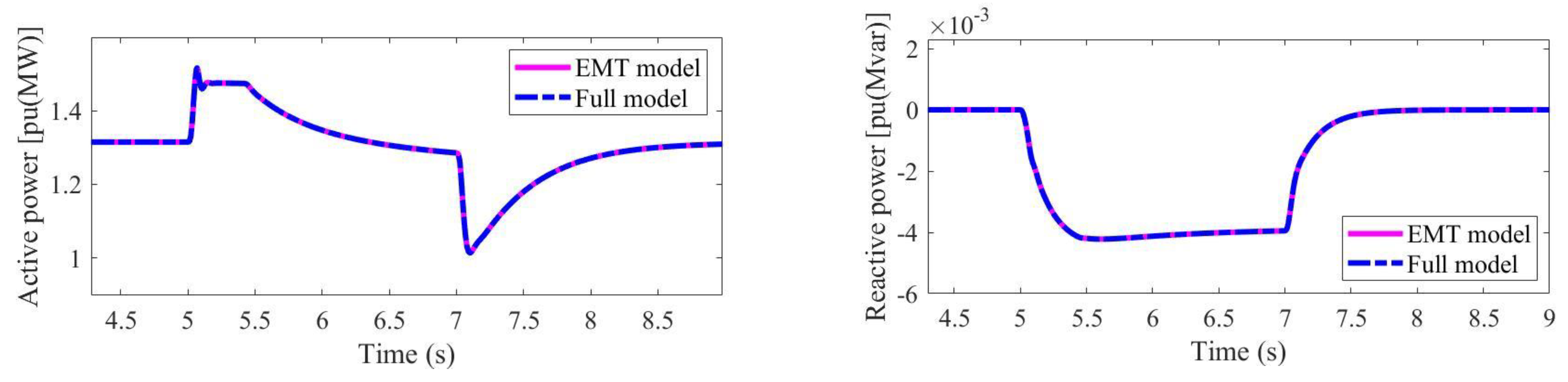
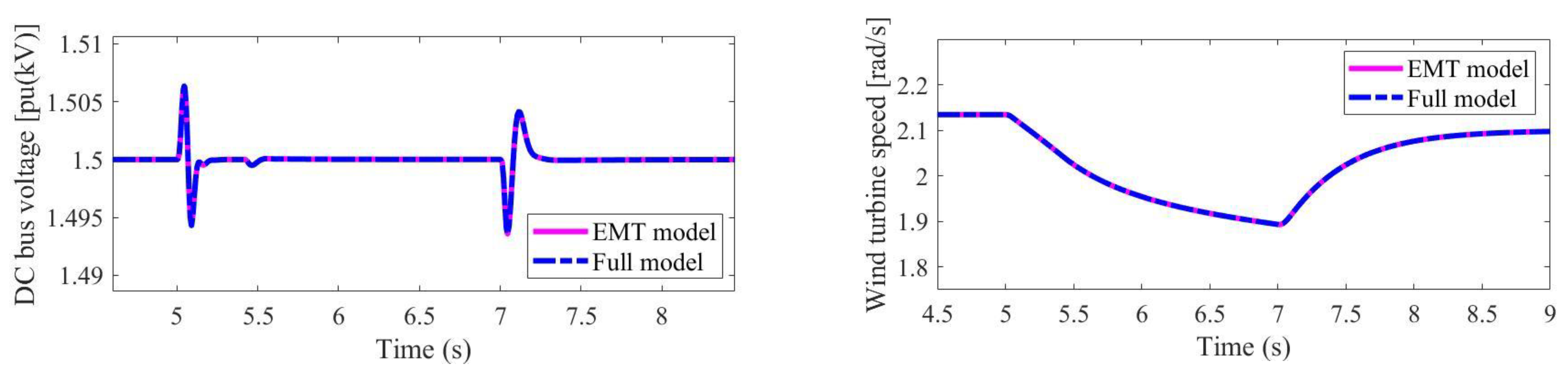
5. Case Study

The D-PMSG model proposed in this paper is mainly used for power system dynamic analysis and power system simulation. For this purpose, this section verifies the accuracy and applicability of the proposed simplified model in the system level. The simulated grid, as shown in Figure 10, is a modified IEEE 39 bus system with three wind plants using 1 MW, 1.5 WM and 2 WM turbines, of which the wind penetration rate is 26.2%. As shown in Figure 10, each wind farm consists of three clusters and each cluster takes up 20%, 30% and 50% of the plant capacity, respectively. For simplicity, it is assumed that in each WPP, the parameters of all the internal D-PMSGs are identical, one of which is given in

Table 3. D-PMSG parameters and settings of WPP1.

Parameter	Value
$S_n$	1 MW
$V_n$	1 kV
$R$	38 m
$V_w$	9.145 m/s
$\rho$	1.225 kg/m3
$H$	5.5 s
$P$	48
${\psi }_p$	1.885 pu
$r_s{/L}_s$	6 × 10−3 pu/9.43 × 10−2 pu
$L_g{/r}_f{/L}_f$	3.14 × 10−2 pu/9.99 × 10−5 pu/3.14 × 10−2 pu
$C_{dc}$	1.04 × 10−4 pu
$V_{dc}$	1.5 pu
$V_g$	0.69 pu
$K_p{/K}_d{/K}_v$	0.833/133.3/0

. Corresponding to the use cases of the D-PMSG model defined in Section 3, three scenarios were considered in this case study: transmission line failure, generator outage and wind speed variation in the wind farm. The simulation was run in DOME, a Python-based power system simulation software [37].

The simulation was executed by a Lenovo Y700 computer with a 4-core Intel i5-6300HQ 2.3 GHz CPU. The computational time for a power system simulation of scenario 1 using the full model, 10ms model and 100 ms D-PMSG model are 27.59 s, 3.63 s and 0.89 s, respectively. By comparison with the full model, using the 10 ms model with the 1 ms time step can speed up the simulation by 86.84%, and using the 100 ms model with the 10 ms time step can speed it up by 96.77%.

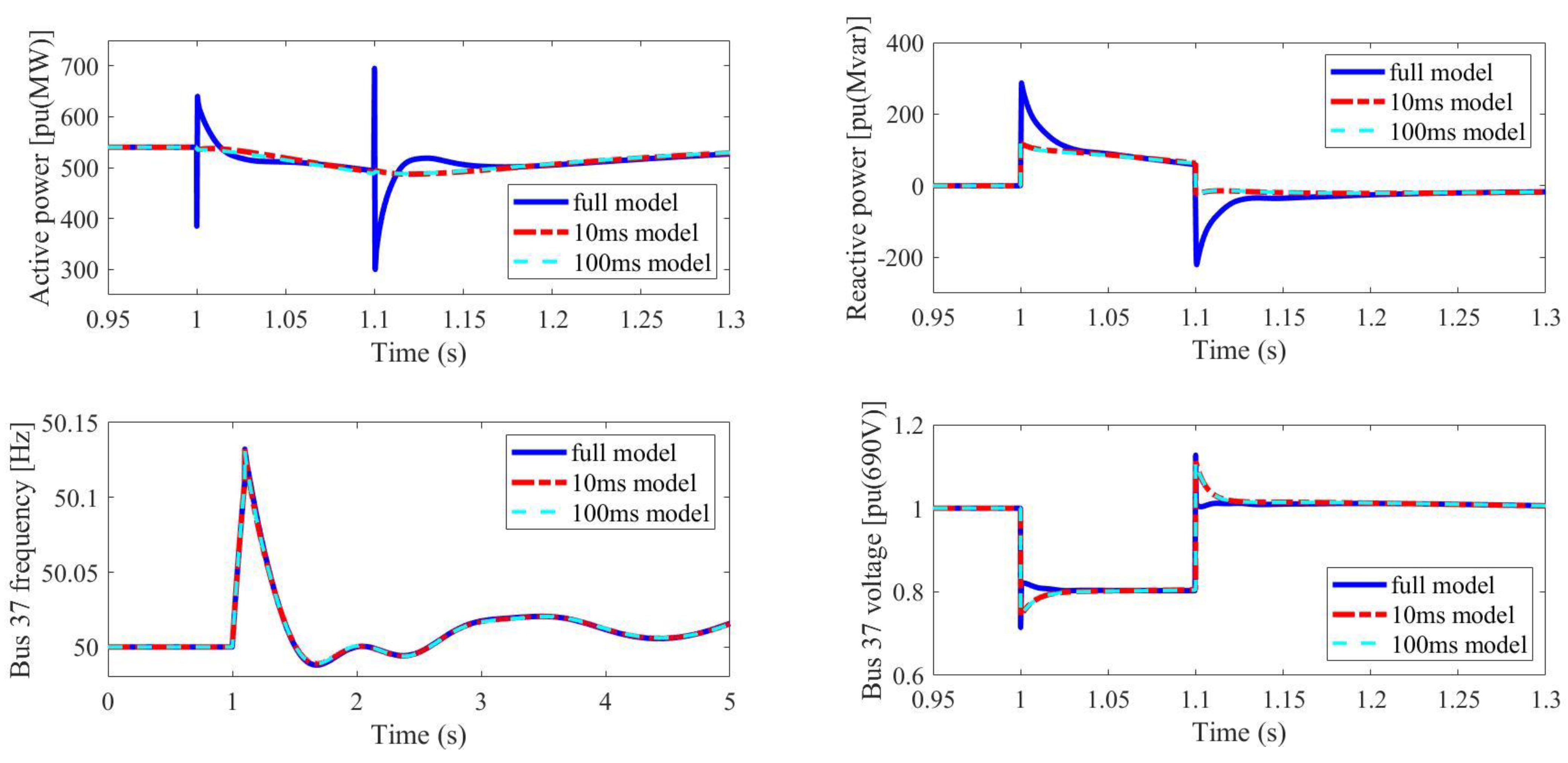
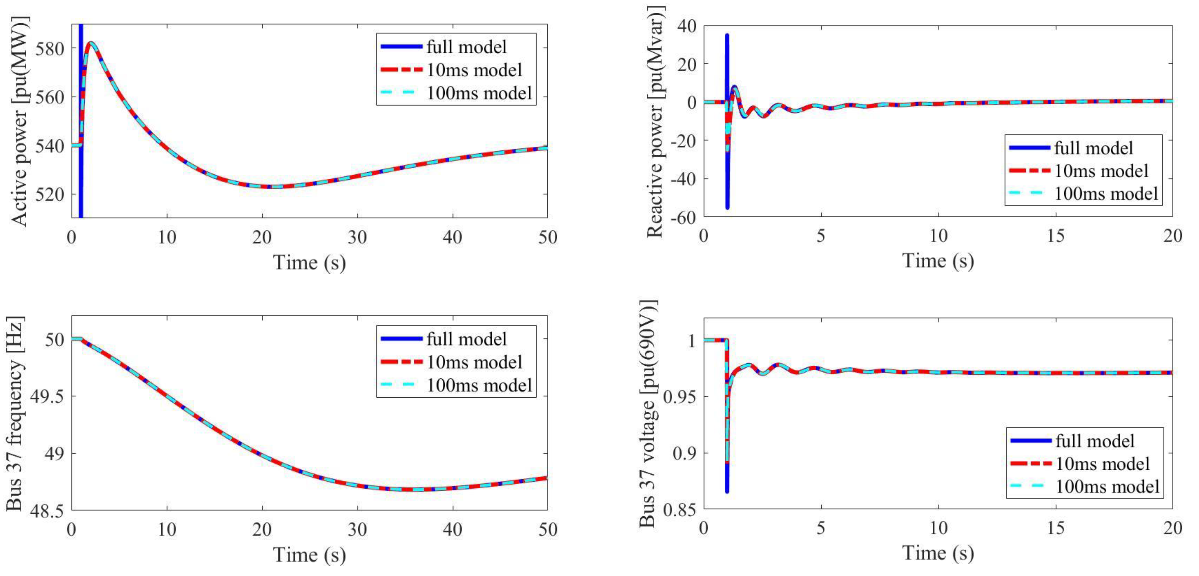
5.1. Scenario 1: Fault

In this section, a fault occurred on the transmission line between bus 1–2 at 1 s and cleared after 100 ms. Figure 11 shows the power response at the point of the grid connection of the wind farm and the system responses in the frequency and voltage. At the moment of fault occurrence and clearance, the system with the full D-PMSG model has a transient peak in the bus voltage. However, the simplified model cannot show such transients because the simplified model ignores the FPC current transients and presents a smooth grid power injection. On the other hand, the response of the system frequency dynamics is the same for all three models, because in this power system the frequency dynamics are mainly driven by the synchronous machines and their controllers. While the penetration increases, it can be expected that the grid frequency would be different between the full model and other models. Therefore, as the use case defined, for the fault analysis, a full model must be used.

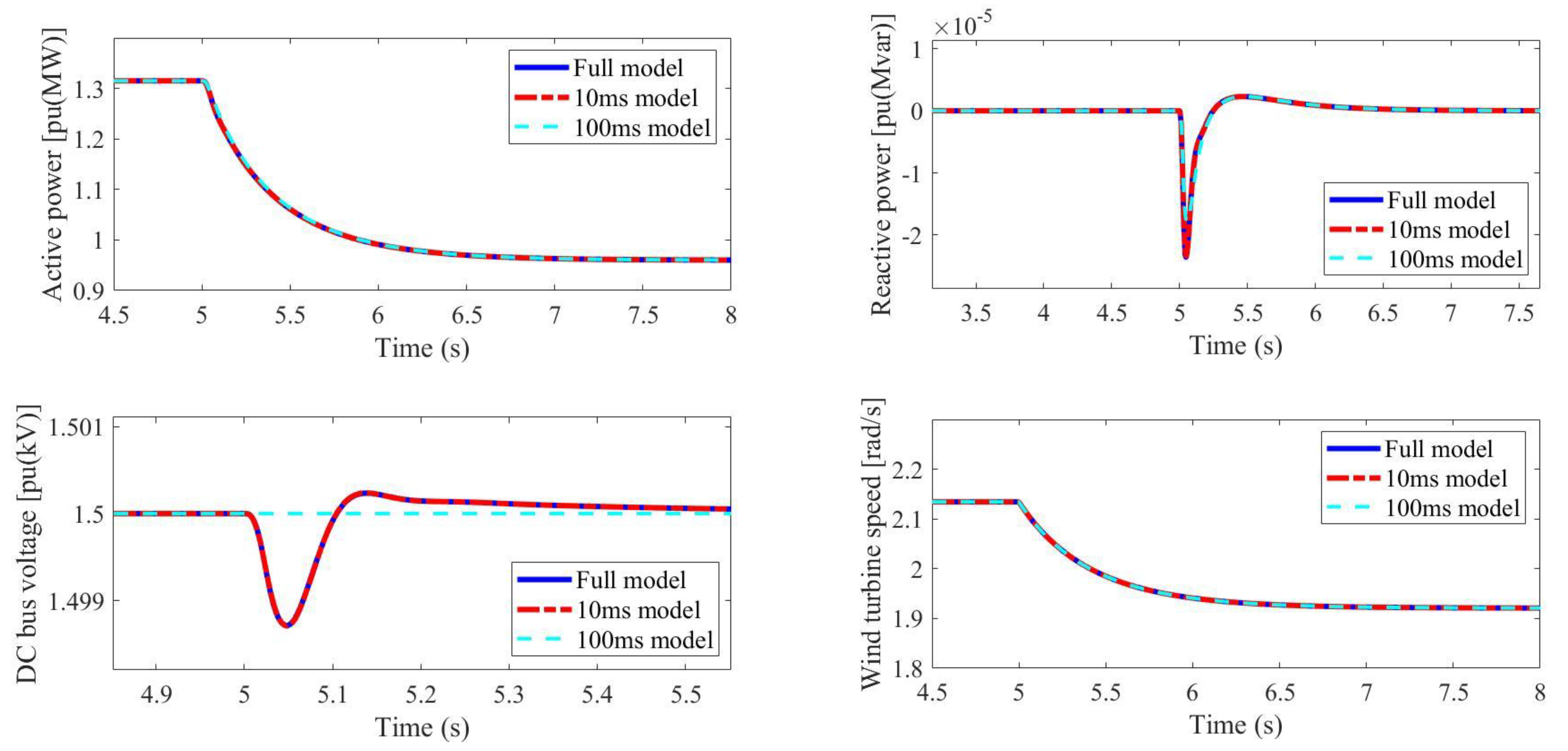
5.2. Scenario 2: Generator Outage

In this scenario, a thermal power plant at bus 34 outages at 1 s. As expected, the 100 ms model can capture all the D-PMSG dynamics in terms of the active and reactive output as shown in Figure 12. Therefore, the 100 ms model can be used in the analysis of the power system frequency and voltage stability.

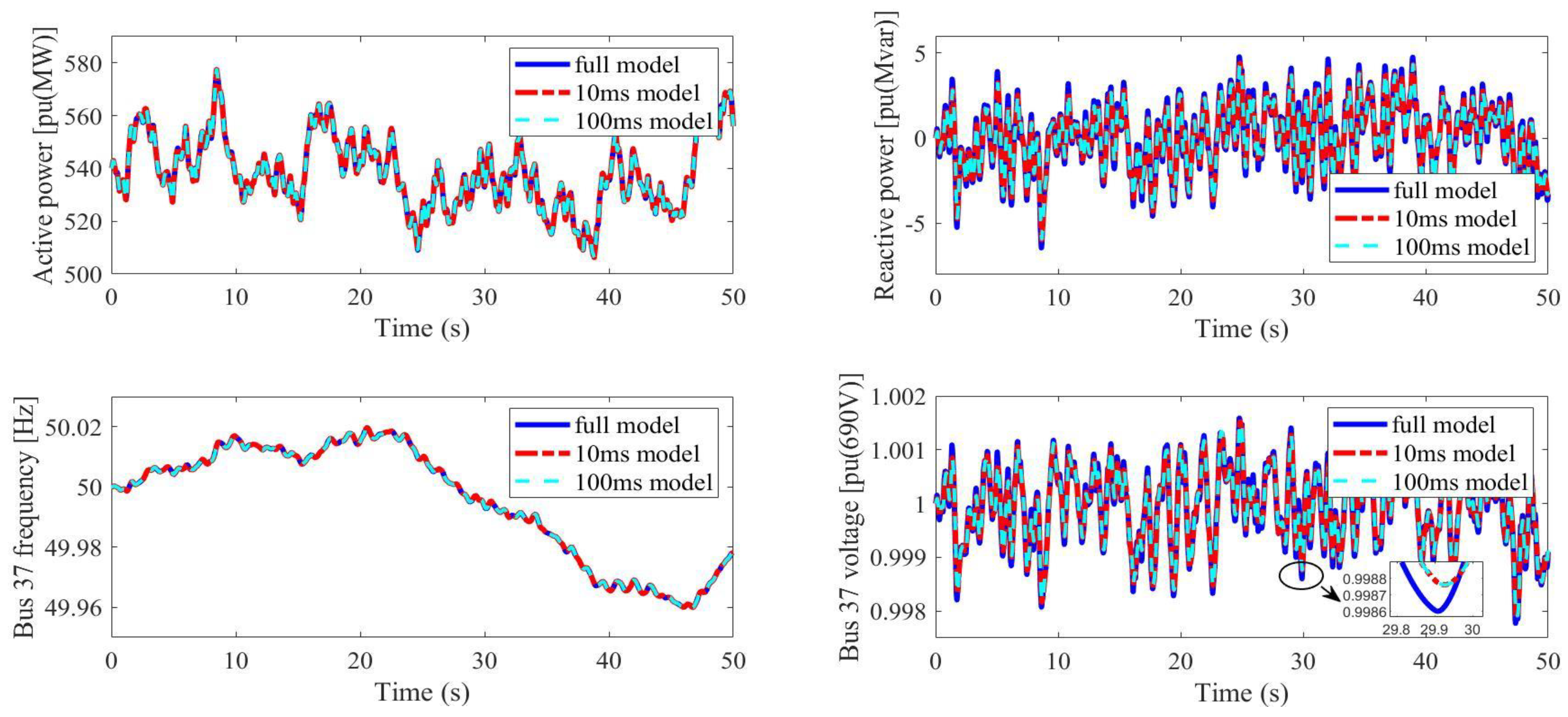
5.3. Scenario 3: Variable Wind Speed

In this scenario (see Figure 13), a Weibull distribution [38] on the wind is under consideration. Since in reality, the wind variant is in the order of the second and the turbine has a certain inertia, the 100 ms D-PMSG model is enough to be used in the power system simulation. The conclusion of the variable wind speed events is similar to that of the system frequency events, so that the 100 ms model is also applicable to the variable wind speed events.

6. Conclusions

This paper proposes a set of D-PMSG models according to the interested timescales of the research. The following conclusions can be drawn:

• In new power systems, the full D-PMSG model must be used for the transient stability or rotor angle stability analysis. The 10 ms model can be used for the voltage stability analysis on both the DC and AC sides. The 100 ms model can fit into the frequency and voltage stability analysis but only on the AC sides.
• For the power system simulation, using D-PMSG 100 ms model can significantly reduce the computation burden while maintaining greater accuracy for the power system dynamic analysis. While for the grid fault or short-circuit analysis, a full D-PMSG model is still needed. In a modified IEEE 39-bus system simulation with 26.2% D-PMSG penetration, using the 100 ms model can save 96.77% of the computational burden in comparison with using the full model.

References

- Sun, C.; Chen, J.; Tang, Z. New Energy Wind Power Development Status and Future Trends. In Proceedings of the 2021 International Conference on Advanced Electrical Equipment and Reliable Operation (AEERO), Beijing, China, 15–17 October 2021; pp. 1–5. [Google Scholar]
- Padmanathan, K.; Kamalakannan, N.; Sanjeevikumar, P.; Blaabjerg, F.; Holm-Nielsen, J.B.; Uma, G.; Arul, R.; Rajesh, R.; Srinivasan, A.; Baskaran, J. Conceptual Framework of Antecedents to Trends on Permanent Magnet Synchronous Generators for Wind Energy Conversion Systems. Energies 2019, 12, 2616. [Google Scholar] [CrossRef] [Green Version]
- Chinchilla, M.; Arnaltes, S.; Burgos, J.C. Control of Permanent-magnet Generators Applied to Variable-speed Wind-energy Systems Connected to the Grid. IEEE Trans. Energy Conver. 2006, 21, 130–135. [Google Scholar] [CrossRef] [Green Version]
- Yin, M.; Li, G.; Zhou, M.; Zhao, C. Modeling of the Wind Turbine with a Permanent Magnet Synchronous Generator for Integration. In Proceedings of the 2007 IEEE Power Engineering Society General Meeting, Tampa, FL, USA, 24–28 June 2007; pp. 1–6. [Google Scholar]
- Ebrahimzadeh, E.; Blaabjerg, F.; Wang, X.; Bak, C.L. Harmonic Stability and Resonance Analysis in Large PMSG-Based Wind Power Plants. IEEE Trans. Sustain. Energ. 2018, 9, 12–23. [Google Scholar] [CrossRef]
- Li, J.; Yang, J.; Xie, X.; Li, H.; Wang, K.; Shi, Z. The effect of different models of closed-loop transfer functions on the inter-harmonic oscillation characteristics of grid-connected PMSG. CSEE J. Power Energy Syst. 2020, 1–8. [Google Scholar] [CrossRef]
- Xie, D.; Lu, Y.; Sun, J.; Gu, C. Small Signal Stability Analysis For Different Types of PMSGs Connected to the Grid. Renew. Energ. 2017, 106, 149–164. [Google Scholar] [CrossRef]
- Du, W.; Dong, W.; Wang, H.F. Small-Signal Stability Limit of a Grid-Connected PMSG Wind Farm Dominated by the Dynamics of PLLs. IEEE Trans. Power Syst. 2020, 35, 2093–2107. [Google Scholar] [CrossRef]
- Cui, Y.; Zeng, P.; Cui, C. Pitch Control Strategy of Permanent Magnet Synchronous Wind Turbine Generator in Response to Cluster Auto Generation Control Command. In Proceedings of the 2019 IEEE Innovative Smart Grid Technologies-Asia (ISGT Asia), Chengdu, China, 21–24 May 2019; pp. 4042–4047. [Google Scholar]
- Alizadeh, O.; Yazdani, A. A Strategy for Real Power Control in a Direct-Drive PMSG-Based Wind Energy Conversion System. IEEE Trans. Power Deliver. 2013, 28, 1297–1305. [Google Scholar] [CrossRef]
- Bouscayrol, A.; Delarue, P.; Guillaud, X. Power strategies for maximum control structure of a wind energy conversion system with a synchronous machine. Renew. Energ. 2005, 30, 2273–2288. [Google Scholar] [CrossRef]
- Esmaili, R.; Xu, L.; Nichols, D.K. A new control method of permanent magnet generator for maximum power tracking in wind turbine application. In Proceedings of the IEEE Power Engineering Society General Meeting, San Francisco, CA, USA, 16 June 2005; pp. 2090–2095. [Google Scholar]
- Qin, S.; Chang, Y.; Xie, Z.; Li, S. Improved Virtual Inertia of PMSG-Based Wind Turbines Based on Multi-Objective Model-Predictive Control. Energies 2021, 14, 3612. [Google Scholar] [CrossRef]
- Morren, J.; De Haan, S.W.; Kling, W.L.; Ferreira, J.A. Wind turbines emulating inertia and supporting primary frequency control. IEEE Trans. Power Syst. 2006, 21, 433–434. [Google Scholar] [CrossRef]
- Keung, P.-K.; Li, P.; Banakar, H.; Ooi, B.T. Kinetic Energy of Wind-Turbine Generators for System Frequency Support. IEEE Trans. Power Syst. 2009, 24, 279–287. [Google Scholar] [CrossRef]
- He, X.; Geng, H.; Mu, G. Modeling of wind turbine generators for power system stability studies: A review. Renew. Sust. Energ. Rev. 2021, 143, 110865. [Google Scholar] [CrossRef]
- Chen, W.; Wang, D.; Xie, X.; Ma, J.; Bi, T. Identification of modeling boundaries for SSR studies in series compensated power networks. IEEE Trans. Power Syst. 2017, 32, 4851–4860. [Google Scholar] [CrossRef]
- Shi, Q.; Wang, F.; Fu, L.; Yuan, L.; Huang, H. State-space averaging model of wind turbine with PMSG and its virtual inertia control. In Proceedings of the IECON 2013-39th Annual Conference of the IEEE Industrial Electronics Society, Vienna, Austria, 10–13 November 2013; pp. 1880–1886. [Google Scholar]
- Shen, Y.; Zhang, J.; Chen, Y.; Pi, A.; Mao, X.; Wang, D.; Zuo, J.; Cui, T. Electromagnetic Transient Model and Parameters Identification of PMSG-Based Wind Farm. In Proceedings of the 2019 IEEE 3rd Conference on Energy Internet and Energy System Integration (EI2), Changsha, China, 8–10 November 2019; pp. 72–77. [Google Scholar]
- Liu, H.; Chen, Z. Aggregated Modelling for Wind Farms for Power System Transient Stability Studies. In Proceedings of the 2012 Asia-Pacific Power and Energy Engineering Conference, Shanghai, China, 27–29 March 2012; pp. 1–6. [Google Scholar]
- Liu, Z.; Wang, L.; Li, N.; Song, J. Performance analysis and model comparison of PMSG for power system transient stability studies. In Proceedings of the 2016 IEEE International Conference on Power and Renewable Energy (ICPRE), Shanghai, China, 21–23 October 2016; pp. 294–300. [Google Scholar]
- Alepuz, S.; Calle, A.; Busquets, M.S.; Kouro, S.; Wu, B. Use of stored energy in PMSG rotor inertia for low-voltage ride-through in back-to-back NPC converter-based wind power systems. IEEE Tran. Ind. Electron. 2013, 60, 1788–1796. [Google Scholar] [CrossRef]
- Conroy, J.; Watson, R. Aggregate modelling of wind farms containing full-converter wind turbine generators with permanent magnet synchronous machines: Transient stability studies. IET Renew. Power Gener. 2009, 3, 39–52. [Google Scholar] [CrossRef]
- Ellis, A.; Kazachkov, Y.; Muljadi, E.; Pourbeik, P.; Sanchez-Gasca, J.J. Description and technical specifications for generic WTG models—A status report. In Proceedings of the 2011 IEEE/PES Power Systems Conference and Exposition, Phoenix, AZ, USA, 20–23 March 2011; pp. 1–8. [Google Scholar]
- Ju, K.; Wu, F.; Shi, L.; Huang, H.; Hua, W.; He, W.; Hua, G. Simplified modeling of Directly Driven Wind Turbine with Permanent Magnet Synchronous Generator based on PSASP/UD. In Proceedings of the 2019 IEEE Innovative Smart Grid Technologies-Asia (ISGT Asia), Chengdu, China, 21–24 May 2019; pp. 1254–1259. [Google Scholar]
- Chen, W.; Feng, B.; Tan, Z.; Wu, N.; Song, F. Intelligent fault diagnosis framework of microgrid based on cloud–edge integration. Energy Rep. 2022, 8, 131–139. [Google Scholar] [CrossRef]
- Xu, L.; Wang, G.; Fu, L.; Wu, Y.; Shi, Q. General average model of D-PMSG and its application with virtual inertia control. In Proceedings of the 2015 IEEE International Conference on Mechatronics and Automation (ICMA), Beijing, China, 2–5 August 2015; pp. 802–807. [Google Scholar]
- Vidyanandan, K.V.; Senroy, N. Primary frequency regulation by deloaded wind turbines using variable droop. IEEE Trans. Power Syst. 2013, 28, 837–846. [Google Scholar] [CrossRef]
- Kang, L.; Shi, L.; Ni, Y.; Yao, L.; Masoud, B. Small signal stability analysis with penetration of grid-connected wind farm of PMSG type. In Proceedings of the 2011 International Conference on Advanced Power System Automation and Protection, Beijing, China, 16–20 October 2011; pp. 147–151. [Google Scholar]
- Ding, N.; Lu, Z.; Qiao, Y.; Min, Y. Simplified equivalent models of large-scale wind power and their application on small-signal stability. J. Mod. Power Syst. Cle. 2013, 1, 58–64. [Google Scholar] [CrossRef] [Green Version]
- Luo, J.; Shi, L.; Ni, Y. A Solution of Optimal Power Flow Incorporating Wind Generation and Power Grid Uncertainties. IEEE Access 2018, 6, 19681–19690. [Google Scholar] [CrossRef]
- Chen, J.J.; Wu, Q.H. Probability interval optimization for optimal power flow considering wind power integrated. In Proceedings of the 2016 International Conference on Probabilistic Methods Applied to Power Systems (PMAPS), Beijing, China, 16–20 October 2016; pp. 1–5. [Google Scholar]
- Wang, R.; Xie, Y.; Zhang, H.; Li, C.; Li, W.; Terzija, V. Dynamic power flow algorithm considering frequency regulation of wind power generators. IET Renew. Power Gen. 2017, 11, 1218–1225. [Google Scholar] [CrossRef]
- Chen, J.; Liu, M.; Donnell, T.O.; Milano, F. Modeling of Smart Transformers for Power System Transient Stability Analysis. IEEE J. Emerg. Sel. Top. Power Electron. 2022, 10, 3759–3770. [Google Scholar] [CrossRef]
- Carne, G.D.; Langwasser, M.; Ndreko, M.; Bachmann, R.; Doncker, R.W.D.; Dimitrovski, R.; Mortimer, B.J.; Neufeld, A.; Rojas, F.; Liserre, M. Which deepness class is suited for modeling power electronics?: A guide for choosing the right model for grid-integration studies. IEEE Ind. Electron. Mag. 2019, 13, 41–55. [Google Scholar] [CrossRef]
- Bunjongjit, K.; Kumsuwan, Y. Performance enhancement of PMSG systems with control of generator-side converter using d-axis stator current controller. In Proceedings of the 2013 10th International Conference on Electrical Engineering/Electronics, Computer, Telecommunications and Information Technology, Krabi, Thailand, 15–17 May 2013; pp. 1–5. [Google Scholar]
- Milano, F. A python-based software tool for power system analysis. In Proceedings of the 2013 IEEE Power & Energy Society General Meeting, Vancouver, BC, Canada, 21–25 July 2013. [Google Scholar]
- Wang, R.; Li, W.; Bagen, B. Development of Wind Speed Forecasting Model Based on the Weibull Probability Distribution. In Proceedings of the 2011 International Conference on Computer Distributed Control and Intelligent Environmental Monitoring, Changsha, China, 19–20 February 2011; pp. 2062–2065. [Google Scholar]