Different Fuzzy Control Configurations Tuned by the Bees Algorithm for LFC of Two-Area Power System ^†

Abstract

This study develops and implements a design of the Fuzzy Proportional Integral Derivative with filtered derivative mode (Fuzzy PIDF) for Load Frequency Control (LFC) of a two-area interconnected power system. To attain the optimal values of the proposed structure’s parameters which guarantee the best possible performance, the Bees Algorithm (BA) and other optimisation tools are used to accomplish this task. A Step Load Perturbation (SLP) of 0.2 pu is applied in area one to examine the dynamic performance of the system with the proposed controller employed as the LFC system. The supremacy of Fuzzy PIDF is proven by comparing the results with those of previous studies for the same power system. As the designed controller is required to provide reliable performance, this study is further extended to propose three different fuzzy control configurations that offer higher reliability, namely Fuzzy Cascade PI − PD, Fuzzy PI plus Fuzzy PD, and Fuzzy (PI + PD), optimized by the BA for the LFC for the same dual-area power system. Moreover, an extensive examination of the robustness of these structures towards the parametric uncertainties of the investigated power system, considering thirteen cases, is carried out. The simulation results indicate that the contribution of the BA tuned the proposed fuzzy control structures in alleviating the overshoot, undershoot, and the settling time of the frequency in both areas and the tie-line power oscillations. Based on the obtained results, it is revealed that the lowest drop of the frequency in area one is −0.0414 Hz, which is achieved by the proposed Fuzzy PIDF tuned by the BA. It is also divulged that the proposed techniques, as was evidenced by their performance, offer a good transient response, a considerable capability for disturbance rejection, and an insensitivity towards the parametric uncertainty of the controlled system.

1. Introduction

Modern large power systems normally comprise multiple interconnected control areas that are based on diverse energy resources. It is extensively reported that any mismatch between the generated power and customer demand results in a deviation in the frequency and tie-line power interchange [1,2,3,4]. This deviation in some cases may lead to system performance degradation and even cause the power systems to collapse [5]. Load Frequency Control (LFC) is introduced in power systems as a key service that plays its role in maintaining the frequency and tie-line power within scheduled limits in normal conditions as well as in the event of any sudden disturbance. This results in the improvement of the stability of the power systems, forming a successful operation [6,7].

In classical LFC applications, the Proportional Integral (PI) and Proportional Integral Derivative (PID) controllers are commonly utilised. The classical PID with a filtered derivative mode optimized by an improved version of the Jaya algorithm, called the Self-Adaptive Multi-Population Elitist (SAMPE) Jaya optimizer, is proposed for the LFC in a two-area interconnected power system [8]. A novel Predictive Functional Modified PID (PFMPID), tuned by the Grasshopper Optimization Algorithm (GOA), is suggested to solve the LFC problem in a three-area power system under a restructured environment and including various generation units. Simulation results demonstrated that the proposed PFMPID outperformed the classical PID [9]. A cascade of PI and PD with a filtered derivative action (PI − PDn) tuned by an Enhanced Coyote Optimization Algorithm (ECOA), equipped in a dual-area power system that consists of a photovoltaic (PV) unit to overcome the problem of frequency and tie-line power deviation, is studied in [10]. The proposed PI − PDn has shown a great superiority over the other investigated controllers. However, due to the escalating complexities with high nonlinearities in current power systems, investigations into the possibility of applying other control techniques are necessitated [11]. Accordingly, several studies have proposed many strategies based on different control theories to address the challenges of the LFC in power systems. For example, Model Predictive Control (MPC) is employed for the LFC in a two-area power system that comprises a photovoltaic generation unit [12]. Sliding Mode Control (SMC) is used for the LFC in a simplified Great Britain (GB) power system [13]. In [14], a novel adaptive sliding mode control method is proposed for the LFC in a three-equal-area interconnected power system with non-reheat turbines; this design demonstrated a better performance in comparison with the classical adaptive sliding mode control scheme. A discrete LFC method has been suggested for power systems with a high penetration of wind power, based on a sampled-data control; this technique has been examined in a single-area power system, a dual-area interconnected power system, and a three-area restricted power system [15]. A Linear Matrix Inequality (LMI)-based LFC with a communication delay in a two-area electrical system is investigated in [16]. ${\mathrm{H}}_{\infty }$ control is used in an isolated, distributed generation system for load frequency control [17]. Moreover, due to its merits, Fuzzy Logic Control (FLC) has recently been widely addressed as a potential solution for LFC based on different structures. It is revealed that FLC can successfully handle the problem of load frequency control. However, there was no identified rule to be utilised in order to find the fuzzy parameters, i.e., the scaling factors of the inputs and outputs as well as the membership functions and the rule base [7]. Therefore, soft computing methods have emerged to deal with this issue. In [18], a fuzzy hierarchal scheme, tuned by Particle Swarm Optimization (PSO), is proposed for the LFC in the Great Britain (GB) power system. Differential Evolution (DE) was employed to optimize the parameters of a fuzzy PID with a derivative filter for the LFC in a multi-sourced, deregulated power system [19]. An optimized fuzzy self-tuning PID controller is proposed for the LFC in two- and three-area interconnected power systems [20]. To ameliorate the proposed controller, a Tribe-DE optimization algorithm was utilized to find the optimum values of the scaling factor and the membership function parameters of the fuzzy PID controllers. The fuzzy PID tuned by Teaching Learning Based Optimization (TLBO) for a dual-area power system is studied in [21]. A novel hybrid DE and Pattern Search (PS) has been used to tune the scaling factor gains of fuzzy PI/PID controllers employed for the LFC in a two-area power system [22]. The most recent controllers, based on the different strategies employed for LFCs in power systems, are concluded in [23].

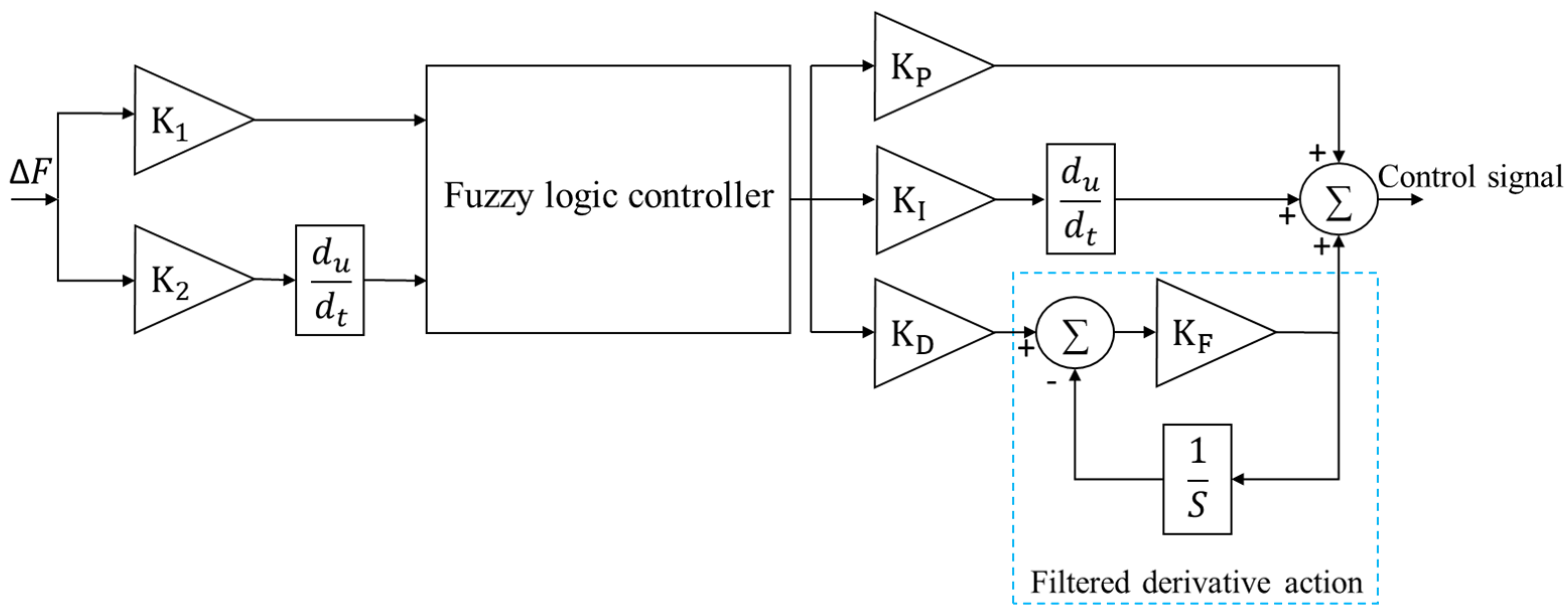
In view of the above, this work proposes a design of a Fuzzy PID with a derivative filter action (Fuzzy PIDF) employed for the LFC in an unequal two-area interconnected thermal power system. Moreover, as the classical methods, including hit and trail, used to determine the optimum values of the scaling factor gains of fuzzy PIDF are time-consuming and may not provide desirable solutions, the parameters of the proposed controller are optimized by an algorithm called the Bees Algorithm (BA), which has demonstrated a successful implementation in diverse optimization problems [24,25,26,27]. TLBO and PSO are also used in this work for the same purpose. The aim of the work presented in this paper can be summarized as follows: (i) to propose a Fuzzy PIDF optimized by the BA and other two algorithms for load frequency control of a two-area power system and to investigate its dynamic performance; (ii) to assess the supremacy of the proposed technique by comparing the results with those of previously published works based on TLBO tuned Fuzzy PID [21] and Lozi map-based Chaotic Optimization Algorithm (LCOA) tuned PID [28]; and (iii) to investigate the robustness of the Fuzzy PIDF against a wide variation range in the parametric uncertainties of the investigated system.

Furthermore, from the comprehensive literature review, it is concluded that the proposed techniques based on different theories may provide the desired performance to overcome the problem of frequency deviation. However, the above-mentioned studies have not considered the reliability aspects in the design of the proposed schemes. This research gap has motivated the authors to suggest fuzzy control configurations for the LFC in power systems that offer different levels of reliability. Therefore, this study is then extended to propose three different fuzzy control structures, namely the Fuzzy Cascade PI − PD, the Fuzzy PI + PD, and the Fuzzy PI plus the Fuzzy PD. An extensive assessment of the robustness of these structures towards the parametric uncertainties of the testbed system, considering thirteen cases, is conducted.

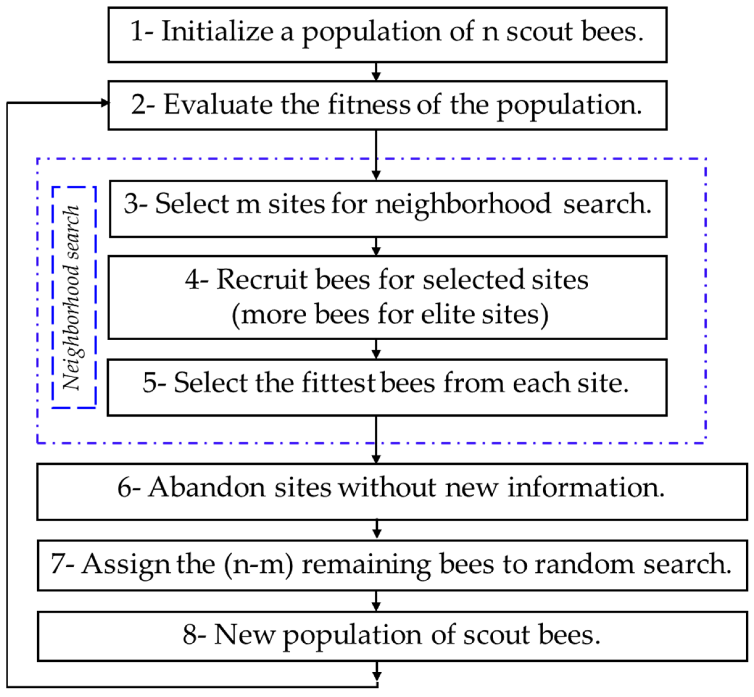
The rest of this study is structured as follows. Section 2 introduces the testbed dual-area interconnected power system. Section 3 details the proposed Fuzzy PID with a filtered derivative action and the employed objective function. Section 4 gives a concise introduction about the suggested optimization technique—the Bees Algorithm. Section 5 details the main simulation results based on the proposed Fuzzy PIDF; this section also provides a comparative study between the Fuzzy PIDF tuned by the BA and the same controller tuned by PSO and TLBO, in addition to other previously published works. Then, Section 6 proposes three novel fuzzy configurations based on the suggested BA, while Section 7 investigates the robustness analyses of the proposed fuzzy structures towards the parametric uncertainties of the testbed system. Lastly, Section 8 encapsulates the main outcomes and proposes a clear path for future works based on this research.

2. Two-Area Power System—Model Understudy

The investigated system in this work is an unequal dual-area, non-reheat interconnected power system, as shown in Figure 1. This system is widely investigated in the literature on the design and analysis of the LFCs of interconnected power systems [21,28].

In this system, the generated mechanical power can be produced by gas, hydraulic, and thermal turbines. The governor senses the generator speed variation and varies the mechanical output power of the turbine by adjusting the position of the turbine input valve; this response is known as the primary frequency response. For stable operation, if the load increases, the governor will decrease the speed; this means moving the turbine input valve to a more open state (this also means increasing the torque). The coefficient of the speed regulation or the droop gain (R) represents the ratio of the frequency deviation to the generator output power variation. The relevant parameters of this model are given in

Table 1. The parameters of the testbed system.

Parameters	Definition	Values in Area 1	Values in Area 2
R	Regulation constant	0.05 MW/Hz	0.0625 MW/Hz
B	Frequency bias	20.6 Hz/MW	16.9 Hz/MW
D	The ratio of change in load to change in frequency	0.6	0.9
H	System inertia time constant	5	4
${\mathrm{T}}_{\mathrm{g}}$	Governor time constant	0.2 s	0.3 s
${\mathrm{T}}_{\mathrm{t}}$	Turbine time constant	0.5 s	0.6 s
T	Synchronization coefficient	2
F	Frequency of the system	60 Hz
SLP	Step Load Perturbation	0.2 pu

.

In order to accomplish the task of the LFC, the term “Area Control Error (ACE)” is usually utilized. The ACE of each area is the input of the proposed fuzzy PIDF. Equations (1) and (2) express the ACEs of area one and area two, respectively. From the control design aspect, the desired operation of large power systems is to maintain the frequency and the tie-line power deviation, fixed on prespecified values, even in the case of load disturbance; this requires the term of ACE to be maintained at zero

$${\mathrm{ACE}}_{\mathrm{area}1}=∆{\mathrm{P}}_{12}+{\mathrm{B}}_1∆{\mathrm{F}}_1$$

(1)

$${\mathrm{ACE}}_{\mathrm{area}2}=∆{\mathrm{P}}_{21}+{\mathrm{B}}_2∆{\mathrm{F}}_2$$

(2)

where $∆{\mathrm{F}}_1$, and $∆{\mathrm{F}}_2$ are the frequency deviation in areas one and two, respectively, $∆{\mathrm{P}}_{12}$ and $∆{\mathrm{P}}_{21}$ are the power flow deviation in areas one and two, and ${\mathrm{B}}_1$ and ${\mathrm{B}}_2$ are frequency biases.

3. Control Strategy and Objective Function

3.1. Fuzzy PIDF Controller

The structural design of the proposed controller equipped in area one is explained in Figure 2. As is evident from the figure, the controller has two inputs, $\mathrm{ACE}1$ and the derivative of $\mathrm{ACE}1$, and one output. In this structure, ${\mathrm{K}}_1$ and ${\mathrm{K}}_2$ are the scaling factor gains of the input. While ${\mathrm{K}}_{\mathrm{P}1},{\mathrm{K}}_{\mathrm{I}1}$, ${\mathrm{K}}_{\mathrm{D}1}$, and ${\mathrm{K}}_{\mathrm{F}1},$ which is the filter gain, are the scaling factors of the output. A similar controller is also employed in area two with ${\mathrm{K}}_3$ and ${\mathrm{K}}_4$ as the input scaling factors and ${\mathrm{K}}_{\mathrm{P}2},{\mathrm{K}}_{\mathrm{I}2}$, ${\mathrm{K}}_{\mathrm{D}2}$, and ${\mathrm{K}}_{\mathrm{F}2}$ for the output scaling gains. Accordingly, twelve parameters are to be optimized to obtain the desired dynamic response of the investigated system. Because of its simplicity and because less computation time is needed for this sort of membership, three triangular/two trapezoidal membership functions are utilized for the inputs and the output variables, as demonstrated in Figure 3, namely Negative Big (NB), Negative Small (NS), Zero (Z), Positive Small (PS), and Positive Big (PB). Therefore, as depicted in

Table 2. Fuzzy rule base of the proposed controller.

$\mathbf{ACE}1$	$\dot{\mathbf{ACE}1}$
	NB	NS	Z	PS	PB
NB	NB	NB	NB	NS	Z
NS	NB	NB	NS	Z	PS
Z	NB	NS	Z	PS	PB
PS	NS	Z	PS	PB	PB
PB	Z	PS	PB	PB	PB

, twenty-five rule bases are required to generate the fuzzy output of the controller. As the controller’s performance depends on these rules, the tabulated rules are obtained by a comprehensive study of the investigated power system’s dynamic behaviour. Furthermore, the “Mamdani” interface method is utilized in this design for the fuzzification stage, while the “Centroid” tool is utilized for the defuzzification stage. Identical membership and rule base are utilised to design the Fuzzy PIDF employed in area two.

3.2. Cost Function

Prior to using the BA, TLBO, and PSO to achieve the best performance of the Fuzzy PIDF employed for the load frequency control in the two-area power system, a proper cost function should be selected. In this paper, the proposed Fuzzy PIDF is designed by minimizing the Integral Time Absolute Error (ITAE) cost function with the aid of the suggested algorithms. The used cost function is expressed in (3). The selection of this cost function is due to the fact that it was proven to reduce both the settling time and the overshoot/undershoot [7].

$$\mathrm{Objective}\mathrm{Function}=\mathrm{ITAE}=\underset{0}{\overset{\mathrm{t}}{{\displaystyle \int }}}\left(\left|∆{\mathrm{F}}_1\right|+\left|∆{\mathrm{F}}_2\right|+\left|∆{\mathrm{P}}_{\mathrm{tie}}\right|\right).\mathrm{t}.\mathrm{dt}$$

(3)

4. The Bees Algorithm (BA)

Since its invention by Pham et al. in 2005 [24], several studies have been introduced based on this algorithm, and different problems in multiple fields have been successfully solved using the BA [24,25,26,27]. It may be worth mentioning that this is one of the first attempts to apply the BA in the field of LFC.

Similar to any optimization algorithm, a number of parameters are required to be set. Specifically, the parameters are the number of scout bees (n); number of sites selected for exploitation out of n visited sites (m); the number of best (elite) sites among the selected sites (e); the number of recruited bees in the best-selected e sites (nep); the number of bees sent to the other (m−e) selected sites (nsp); and the initial size of each patch (ngh) that includes the site and the neighbourhood area as well as the stopping criteria. The simplest pseudo-code for this algorithm is shown in Figure 4.

The mechanism of this algorithm begins with placing the n scout bees randomly in the search space. In step 2, the evaluation of the fitness of the sites visited by the n scout bees is performed. The m sites with the highest fitness in specified “chosen sites” in step 3 are selected for the neighbourhood or local search. The algorithm in steps 4 and 5 conducts searches in the neighbourhood of the selected sites, with more bees assigned to the best e sites. The selection of the best sites could be conducted directly, based on the fitness associated with them. Alternatively, using the fitness values, the probability of the sites being selected is determined. Searches in the neighbourhood of the best e sites which represent the most promising solutions are made more prominent by recruiting more bees for them than for the other selected sites. Together with scouting, this differential recruitment is a key operation of the Bees Algorithm. For each patch, only the one bee that has found the site with the highest fitness (the “fittest” bee) is selected in step 5 to form part of the next bee population. In steps 6–8, the remaining bees in the population n are assigned randomly around the search space to scout for potential new solutions or to conduct the global search. These eight steps are repeated until a stopping criterion is met. The colony will have two parts to its new population at the end of each iteration: representatives from each selected patch and other scout bees assigned to conduct random searches [29].

5. Results and Discussions

This study was carried out in MATLAB (2019a); the Bees Algorithm (BA), Teaching Learning Based Optimisation (TLBO), and Particle Swarm Optimisation (PSO) codes were programmed in (.m files); the examined dual-area power system was built in the MATLAB Simulink environment. The parameters of the BA and the PSO were set as shown in

Table 3. The BA and PSO parameters.

Controller	Parameters
BA	N	m	e	nep	nsp	ngh
	30	12	6	11	7	0.011
PSO	No. Par	${\mathrm{w}}_{\min }$	${\mathrm{w}}_{\max }$	${\mathrm{C}}_1$	${\mathrm{C}}_2$	CR
	30	0.4	0.9	2	2	0.65

. Where ${\mathrm{C}}_1$ and ${\mathrm{C}}_2$ are the acceleration constants, ${\mathrm{w}}_{\min }$ and ${\mathrm{w}}_{\max }$ are the inertia weights, CR is the crossover rate, and No. Par is the number of particles. The TLBO has two parameters to be set, namely the population size and the number of iterations, which were set as 50 and 40, respectively.

A Step Load Perturbation (SLP) of 0.2 pu was applied in area one to study the dynamic performance of the system with the proposed Fuzzy PIDF. The optimum values of the Fuzzy PIDF parameters obtained by the BA, TLBO, and PSO are given in

Table 4. Gains of Fuzzy PIDF controllers tuned by BA, TLBO, and PSO.

Controller	Controller Gains of Area 1						Controller Gains of Area 2
	${\mathbf{K}}_1$	${\mathbf{K}}_2$	${\mathbf{K}}_{\mathbf{P}1}$	${\mathbf{K}}_{\mathbf{I}1}$	${\mathbf{K}}_{\mathbf{D}1}$	${\mathbf{K}}_{\mathbf{F}1}$	${\mathbf{K}}_3$	${\mathbf{K}}_4$	${\mathbf{K}}_{\mathbf{P}2}$	${\mathbf{K}}_{\mathbf{I}2}$	${\mathbf{K}}_{\mathbf{D}2}$	${\mathbf{K}}_{\mathbf{F}2}$
Fuzzy PIDF-BA	0.403	2	2	2	2	98.4841	0.2648	1.0081	0.9133	1.9730	1.9889	93.8922
Fuzzy PIDF-TLBO	0.035	1.9992	1.9986	1.99868	1.9995	99.0606	1.9602	0.03707	0.4435	1.3003	0.019	99.7446
Fuzzy PIDF-PSO	0.02	2	2	2	2	100	2	2	2	0.015	1.4035	11.21

. The scaling factors of the proposed Fuzzy controller design were chosen in the limits of [0,1,2], and the filter coefficient ${\mathrm{K}}_{\mathrm{F}}$ was constrained in the range from 0 to 100.

Moreover, as is above mentioned, the results obtained from the proposed fuzzy structure are compared with those of the previously published studies for the same system investigated in [21] and [28]. The optimum gains of the PID tuned by the LCOA proposed in [28] and the TLBO optimized Fuzzy PID studied in [21] are given in

Table 5. Gains of PID controllers tuned by LCOA and Fuzzy PID controllers tuned by TLBO.

Controller	Controller Gains of Area 1						Controller Gains of Area 2
PID-LCOA [28]	${\mathrm{K}}_{\mathrm{P}1}$		${\mathrm{K}}_{\mathrm{I}1}$		${\mathrm{K}}_{\mathrm{D}1}$		${\mathrm{K}}_{\mathrm{P}2}$		${\mathrm{K}}_{\mathrm{I}2}$		${\mathrm{K}}_{\mathrm{D}2}$
	0.939		0.7998		0.5636		0.5208		0.4775		0.7088
Fuzzy PID-TLBO [21]	${\mathrm{K}}_1$	${\mathrm{K}}_2$		${\mathrm{K}}_3$		${\mathrm{K}}_4$	${\mathrm{K}}_5$	${\mathrm{K}}_6$		${\mathrm{K}}_7$		${\mathrm{K}}_8$
	1.9857	1.9968		1.6870		1.9876	1.3469	1.5512		0.8098		0.5043

.

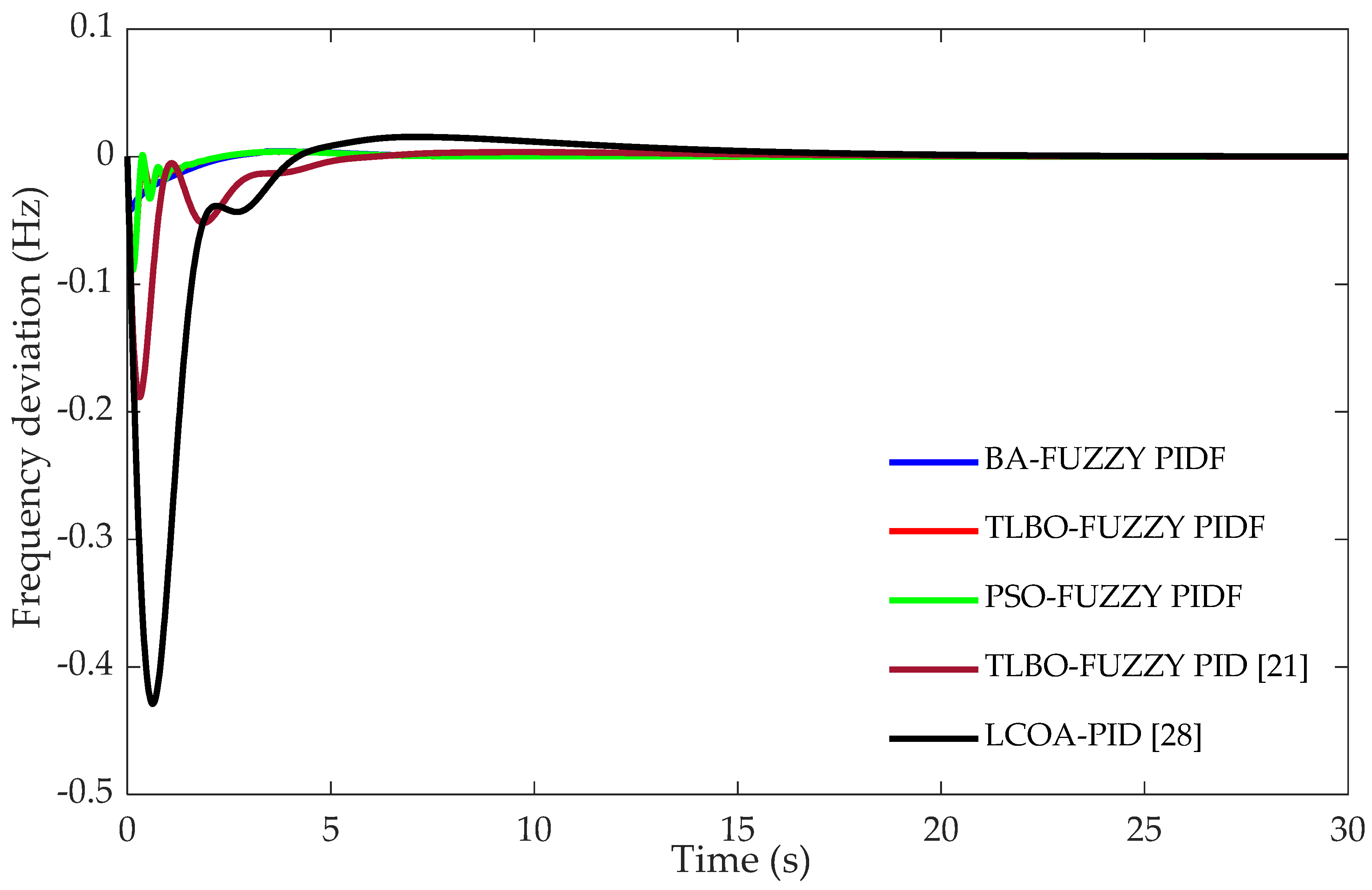
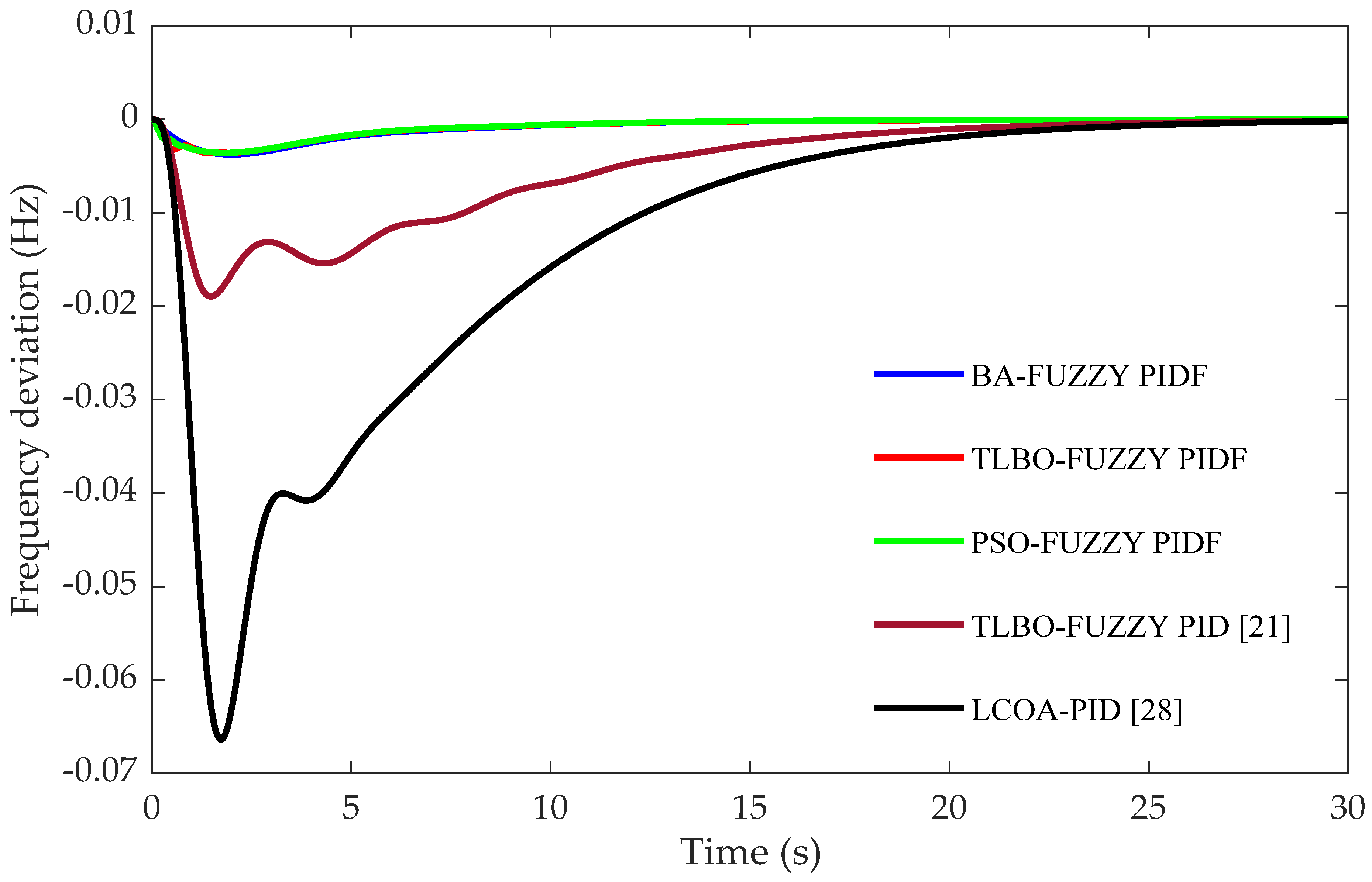
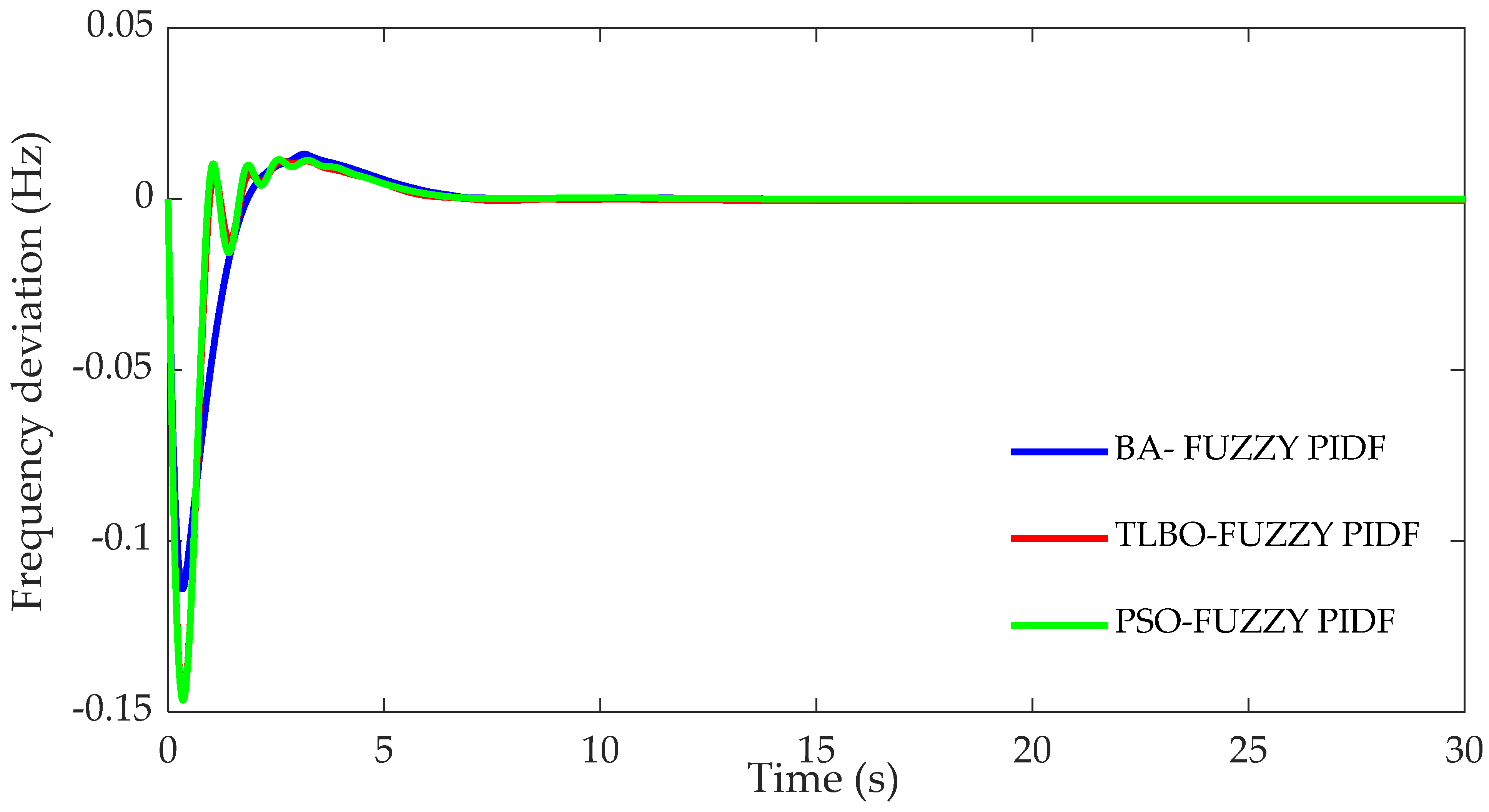
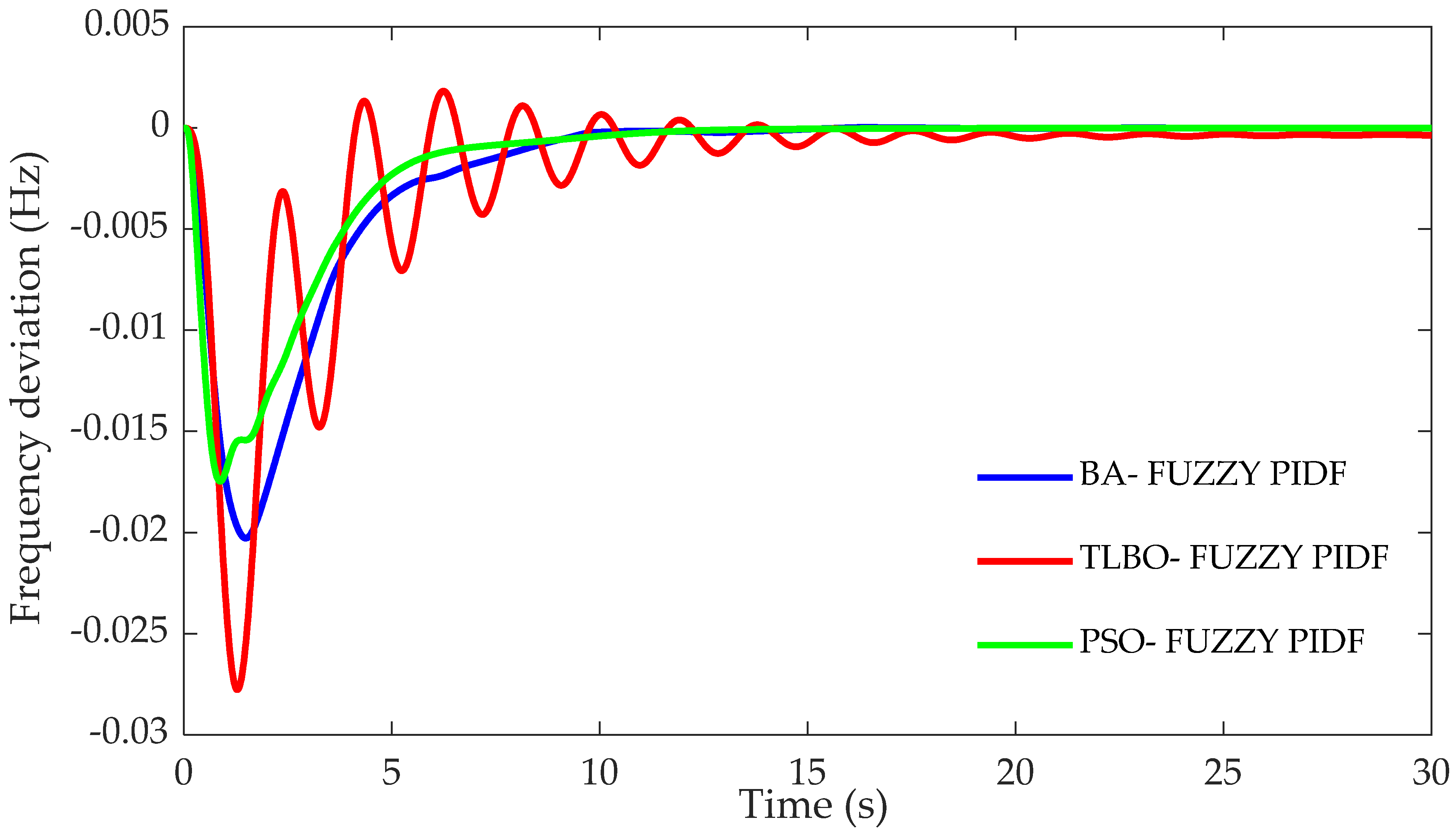
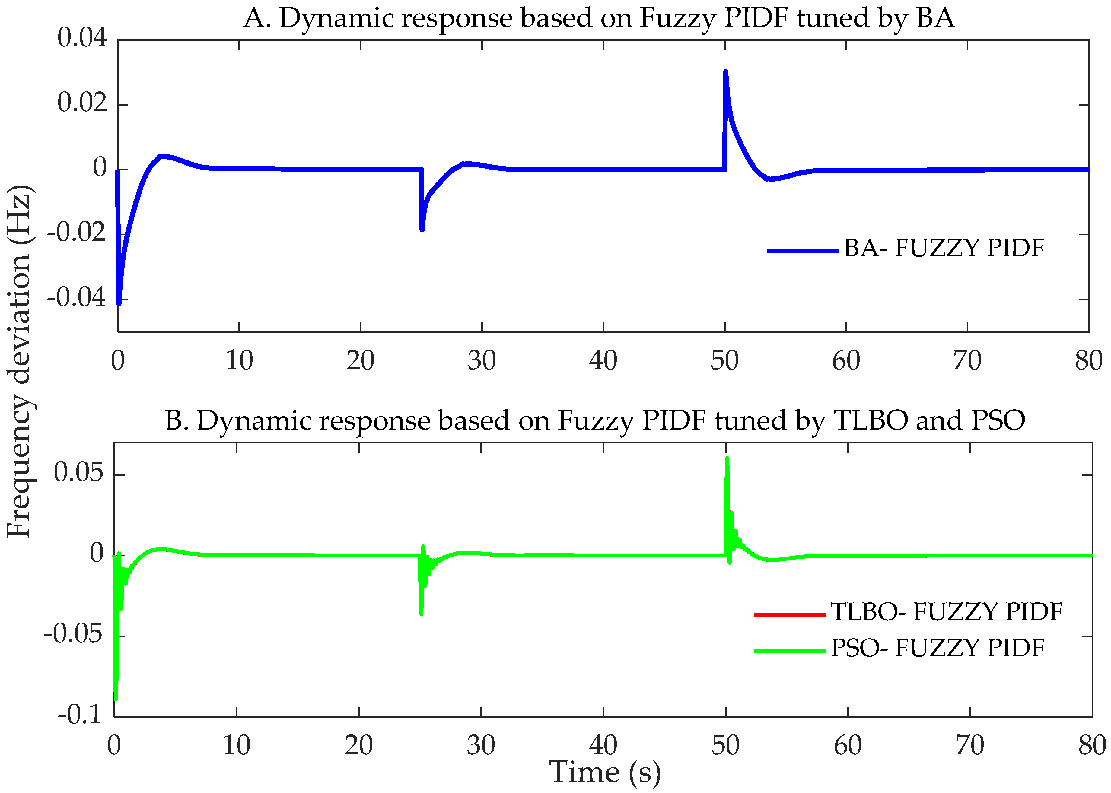
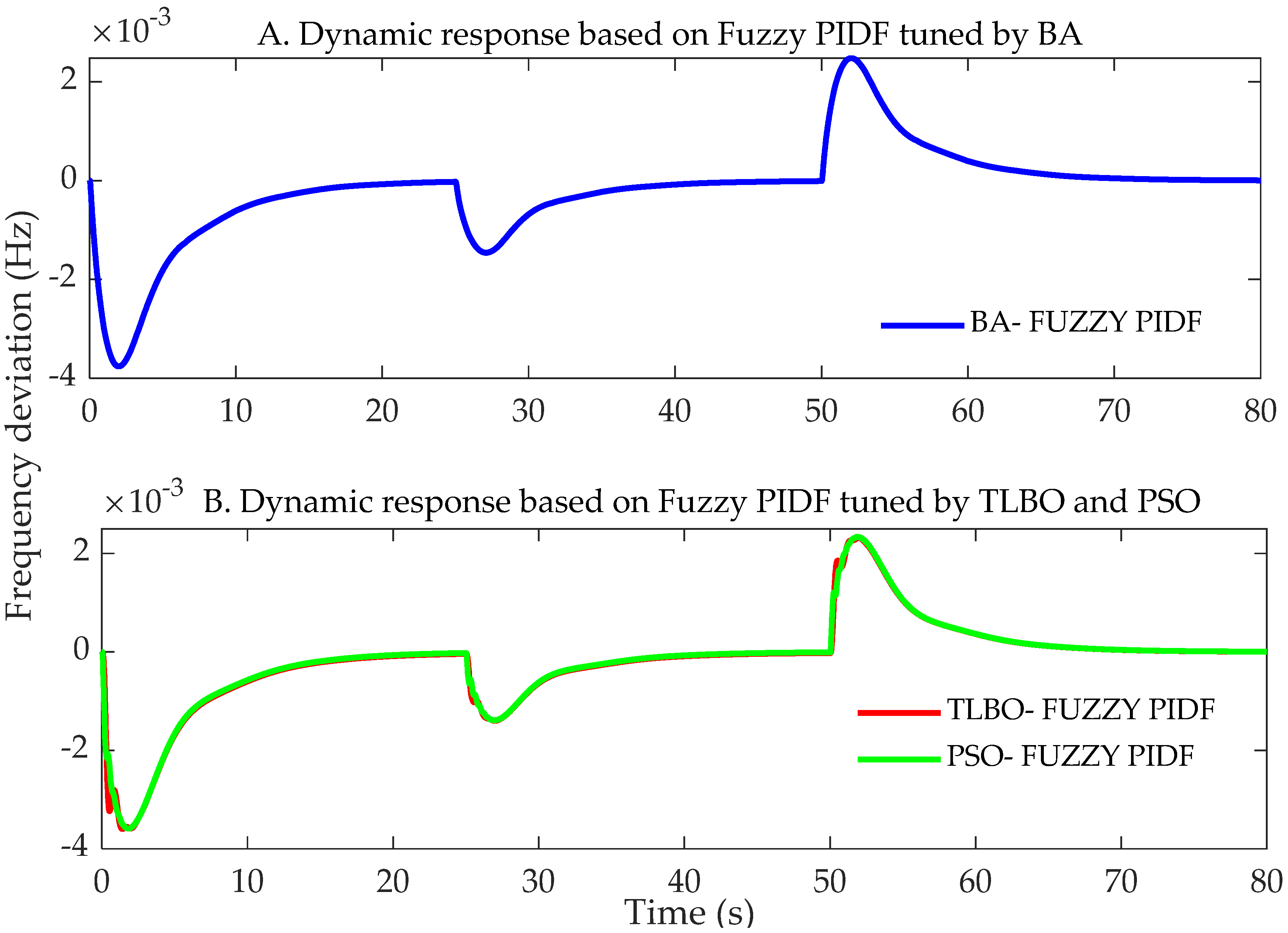
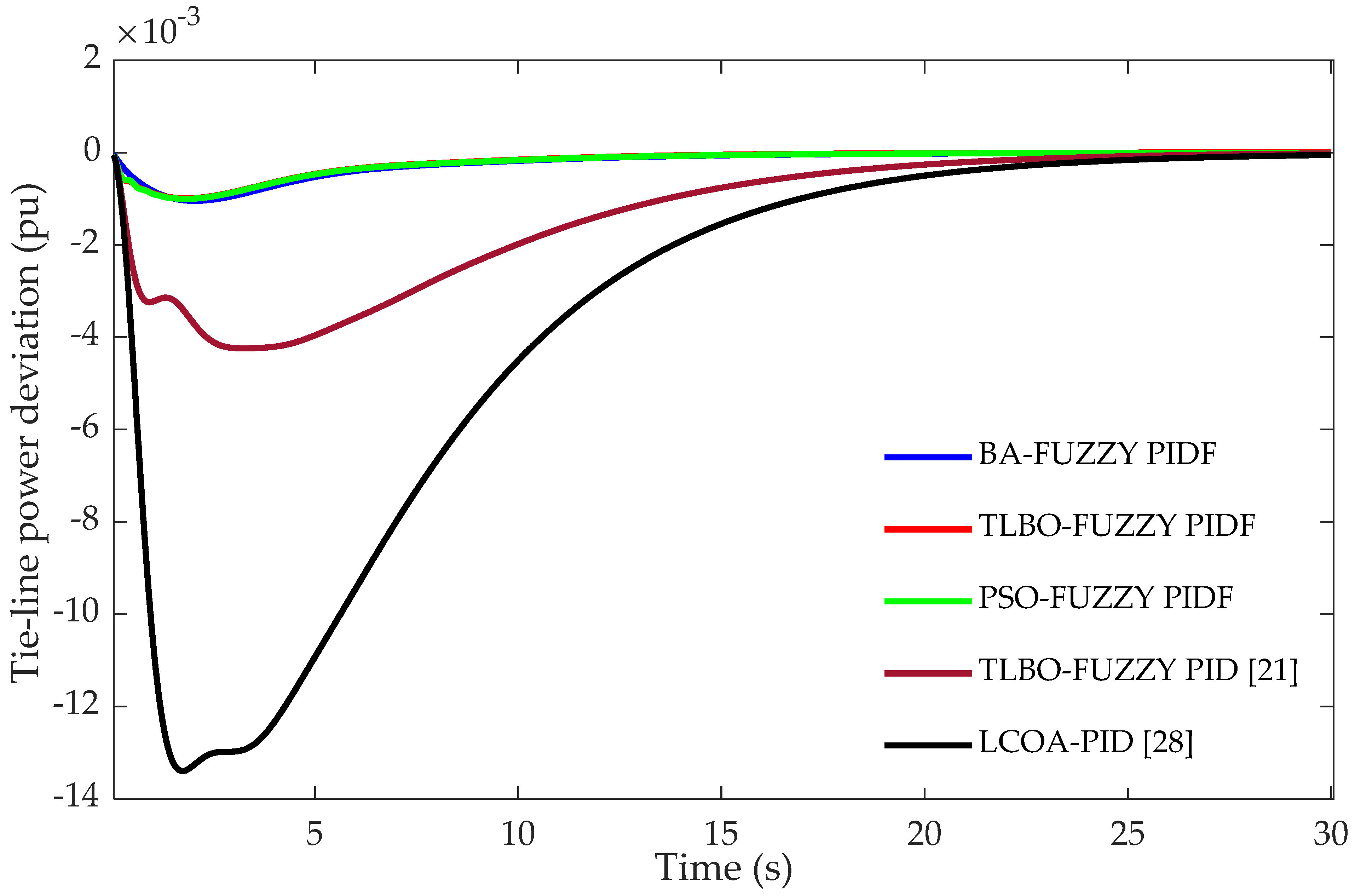
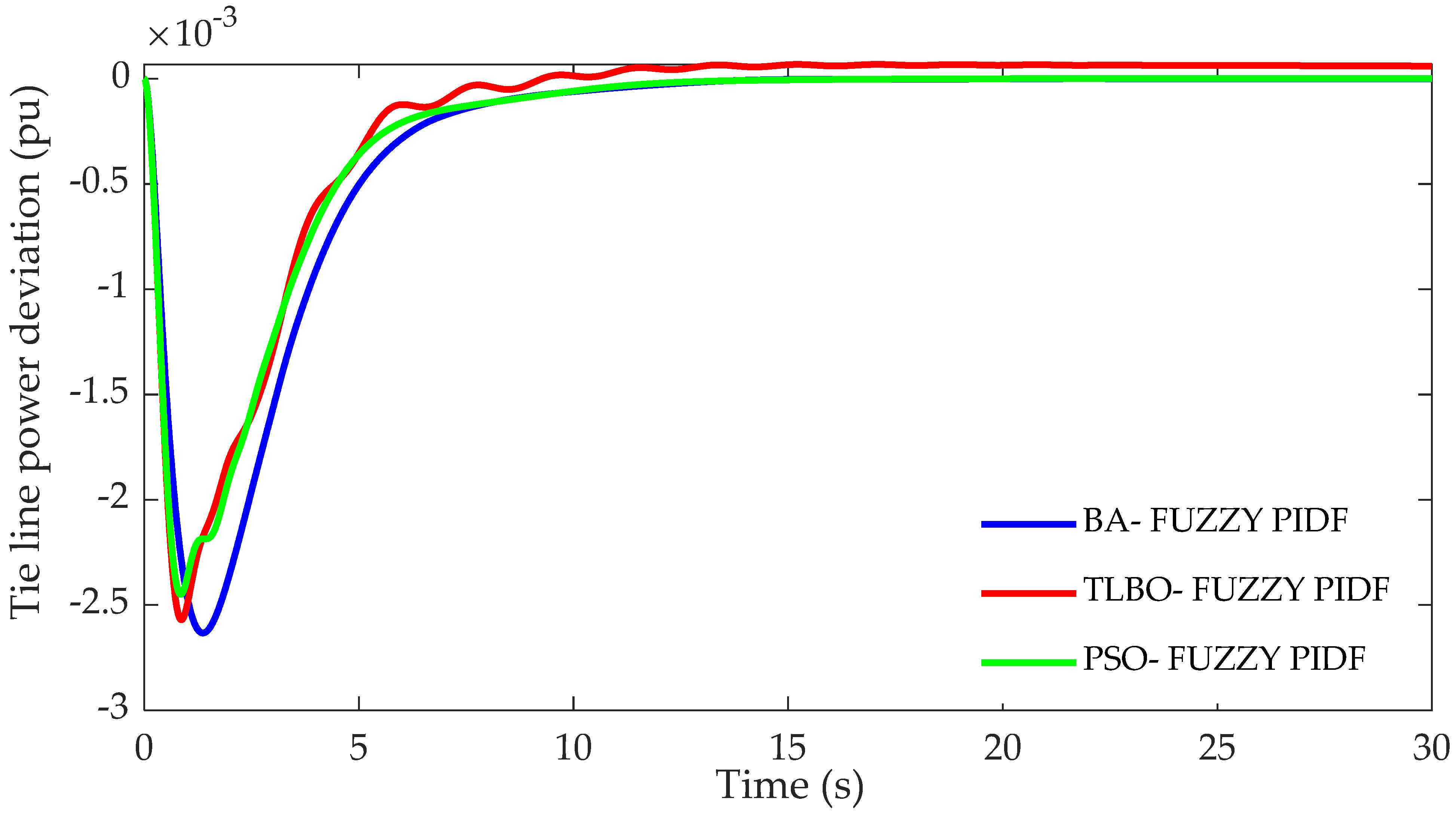
The frequency deviation in both areas, $∆{\mathrm{F}}_1$ and $∆{\mathrm{F}}_2$, following the implementation of 0.2 pu disturbance in area one, is shown in Figure 5 and Figure 6, respectively. The tie-line power deviation is given in Figure 7.

Figure 5, Figure 6 and Figure 7 summarize the main outcomes of the proposed Fuzzy PIDF, where it is obviously remarked that this controller offered the best response among the investigated methods. Furthermore, despite the clear similarity in the dynamic response obtained by the proposed fuzzy structure tuned by BA, TLBO, and PSO, it is observed that the BA optimized the proposed fuzzy controller and provided the best result in terms of the drop in the frequency represented by the peak undershoot occurring in area one after the 0.2 pu disturbance enforcement. However, the Fuzzy PIDF tuned by the TLBO and PSO offered the best drop in frequency in area two. The dynamic performance of the system based on the Fuzzy PIDF tuned by the suggested algorithms, the Fuzzy PID optimized by TLBO, and the PID controller tuned by LCOA, represented by undershoot, peak overshoot, and settling time in $∆{\mathrm{F}}_1$, $∆{\mathrm{F}}_2$, and $∆{\mathrm{P}}_{\mathrm{tie}}$, is illustrated in

Table 6. Characteristics of the testbed system with several controllers.

Controller	Frequency in Area 1			Frequency in Area 2			Tie-Line Power Deviation			ITAE
	${\mathbf{U}}_{\mathbf{sh}}\mathbf{in}\mathbf{Hz}$	${\mathbf{O}}_{\mathbf{sh}}\mathbf{in}\mathbf{Hz}$	${\mathbf{T}}_{\mathbf{s}}\mathbf{in}\mathbf{s}$	${\mathbf{U}}_{\mathbf{sh}}\mathbf{in}\mathbf{Hz}$	${\mathbf{O}}_{\mathbf{sh}}\mathbf{in}\mathbf{Hz}$	${\mathbf{T}}_{\mathbf{s}}\mathbf{in}\mathbf{s}$	${\mathbf{U}}_{\mathbf{sh}}\mathbf{in}\mathbf{pu}$	${\mathbf{O}}_{\mathbf{sh}}\mathbf{in}\mathbf{pu}$	${\mathbf{T}}_{\mathbf{s}}\mathbf{in}\mathbf{s}$
BA-Fuzzy PIDF	0.0414	0.0041	6.9401	0.0038	0	19.2991	0.0010	0	19.360	0.0361
TLBO-Fuzzy PIDF	0.0868	0.0040	5.7544	0.0036	0	19.3273	0.00099	0	18.893	0.0304
PSO-Fuzzy PIDF	0.0890	0.0040	5.7175	0.0036	0	19.1020	0.0010	0	19.154	0.0330
TLBO-Fuzzy [21]	0.1885	0.0036	4.9936	0.019	0	23.5188	0.0042	0	23.937	0.3264
LCOA-PID [28]	0.4288	0.0155	11.703	0.0664	0	21.0698	0.0134	0	21.978	0.7842

; the value of the objective function based on each technique is also given.

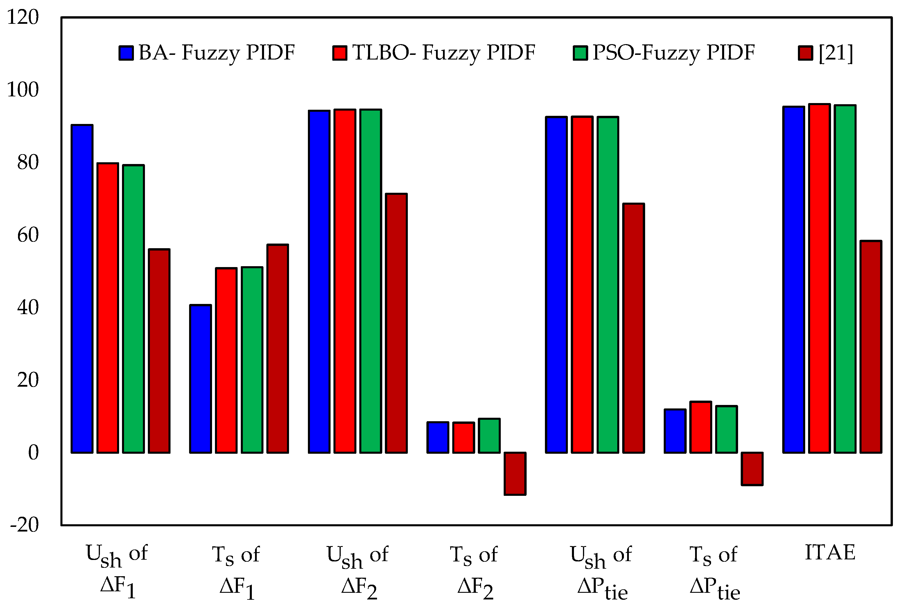
Table 6 gives further verification of the superiority of the suggested controller over those presented in previous studies. The percentage of improvement in the undershoot (${\mathrm{U}}_{\mathrm{sh}}$), settling time (${\mathrm{T}}_{\mathrm{s}}$), and the ITAE for the Fuzzy configuration optimized by different algorithms and the Fuzzy PID proposed in [21], in comparison with the LCOA-based PID controller [28], is shown in Figure 8 (this figure is obtained by analyzing the characteristics provided in Table 6). From Figure 8, it is noted that with the proposed Fuzzy PIDF controller optimized by the suggested algorithms, the overall performance of the system has witnessed a remarkable improvement.

In order to examine the robustness of the Fuzzy PIDF towards the parametric uncertainties of the controlled system, several parameters of the investigated testbed system are simultaneously altered from their nominal values. The parameters Tg, Tt, and H in both areas are varied by +50%, while the parameters B and D are varied by −50%. A step load perturbation of 0.2 pu is suddenly applied (at time t = 0 s) in area one and the optimal gains of the Fuzzy PIDF obtained in the normal condition are not to be re-tuned to verify the robustness of the proposed controller. Figure 9, Figure 10 and Figure 11 and

Table 7. Frequency response performances with different controllers for parametric uncertainties analysis.

Controller	Frequency in Area 1			Frequency in Area 2			Tie-Line Power Deviation			ITAE
	${\mathbf{U}}_{\mathbf{sh}}\mathbf{in}\mathbf{Hz}$	${\mathbf{O}}_{\mathbf{sh}}\mathbf{in}\mathbf{Hz}$	${\mathbf{T}}_{\mathbf{s}}\mathbf{in}\mathbf{s}$	${\mathbf{U}}_{\mathbf{sh}}\mathbf{in}\mathbf{Hz}$	${\mathbf{O}}_{\mathbf{sh}}\mathbf{in}\mathbf{Hz}$	${\mathbf{T}}_{\mathbf{s}}\mathbf{in}\mathbf{s}$	${\mathbf{U}}_{\mathbf{sh}}\mathbf{in}\mathbf{pu}$	${\mathbf{O}}_{\mathbf{sh}}\mathbf{in}\mathbf{pu}$	${\mathbf{T}}_{\mathbf{s}}\mathbf{in}\mathbf{s}$
BA-Fuzzy PIDF	0.1140	0.0131	5.9858	0.0203	0	9.3781	0.0026	0	10.453	0.03094
TLBO-Fuzzy PIDF	0.1458	0.0111	5.4378	0.0278	0.00183	14.818	0.0026	0.000065	9.3769	0.0511
PSO-Fuzzy PIDF	0.1465	0.0115	5.4468	0.0175	0	10.269	0.0024	0	10.421	0.02535

show the dynamic performance of the two-area power system as it is exposed to a parametric deviation test with the recommended Fuzzy PIDF-based BA, TLBO, and PSO employed for LFC.

The results obtained from the robustness analysis demonstrate that the proposed fuzzy structure equipped in the testbed system for the LFC is robust towards the parametric variation of the controlled plant. It is also noticed that the same controller optimized by the TLBO has shown less robustness as compared with the same controller tuned by the BA and the PSO.

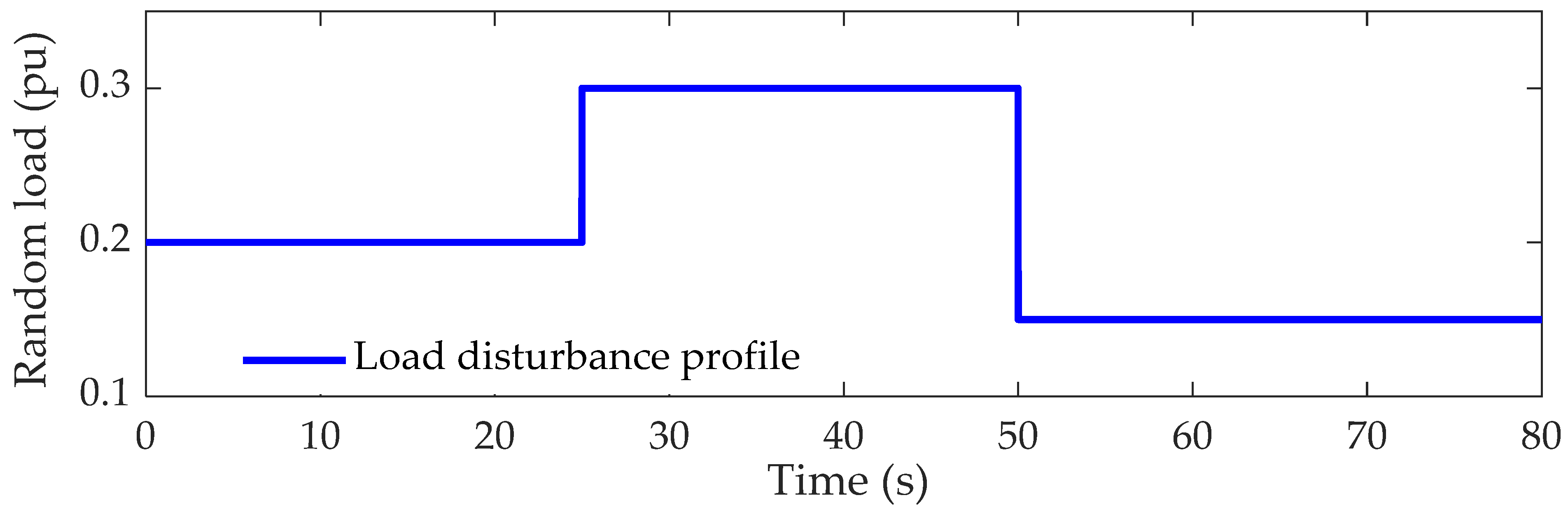
Moreover, for further robustness examination of the proposed fuzzy design at various load perturbations, a random disturbance is applied with a different magnitude in area one, as demonstrated in Figure 12. The dynamic responses of the testbed system when it is exposed to different load disturbances are shown in Figure 13, Figure 14 and Figure 15.

From Figure 13, Figure 14 and Figure 15, it is noticeable that the optimized fuzzy control structure continued to demonstrate its robustness even with random load disturbance applied in the system. Moreover, it is observed that the Fuzzy PIDF-based BA offers the best response as less peak undershoot and less oscillation are achieved in comparison with the same controller-based PSO and TLBO.

6. Different Configurations of Fuzzy Control Tuned by BA

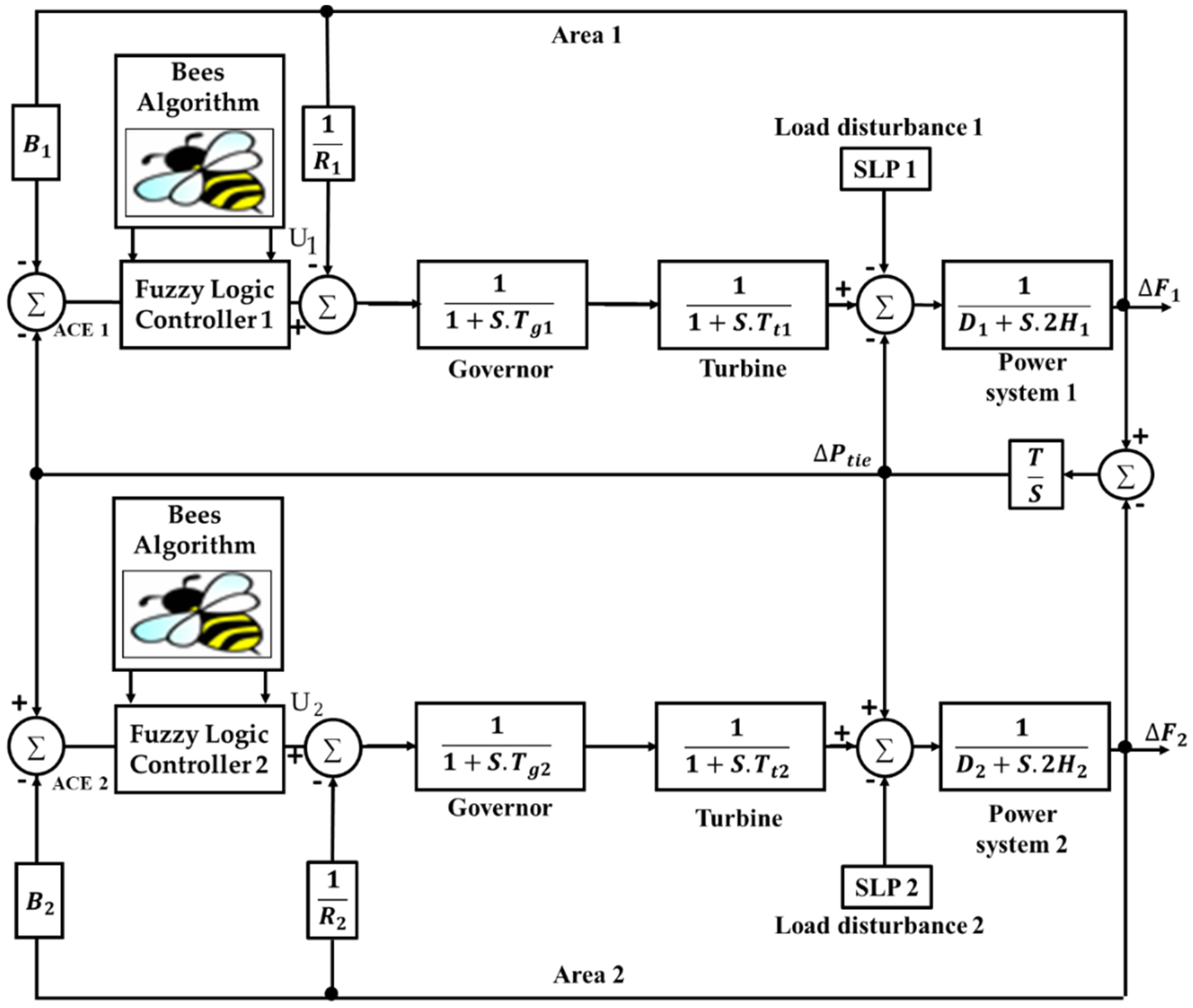
It is revealed that the membership function selection and the setting of the rule base are vital in designing a fuzzy controller. However, it is also a significant matter to investigate the impact of the configuration of the fuzzy controller. This is to explore how different structures of the scaling factor gains influence the performance of the controller. 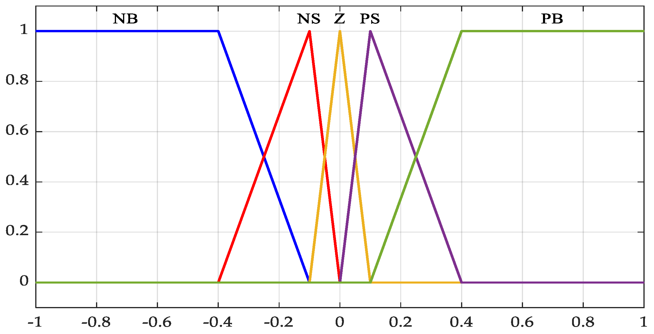Based on this statement, this study is extended to propose three different structures of fuzzy control employed as LFC system for the two-area power system shown in Figure 1. The same membership function used to design the Fuzzy PIDF shown in Figure 3 is used with the proposed structures. Furthermore, the rule bases required to generate the fuzzy output of the controller are tabulated in Table 2.

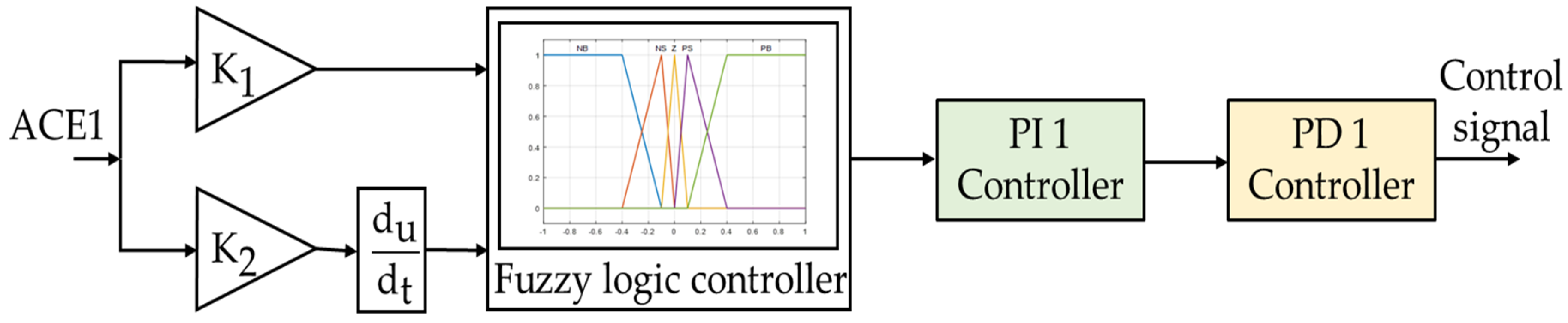
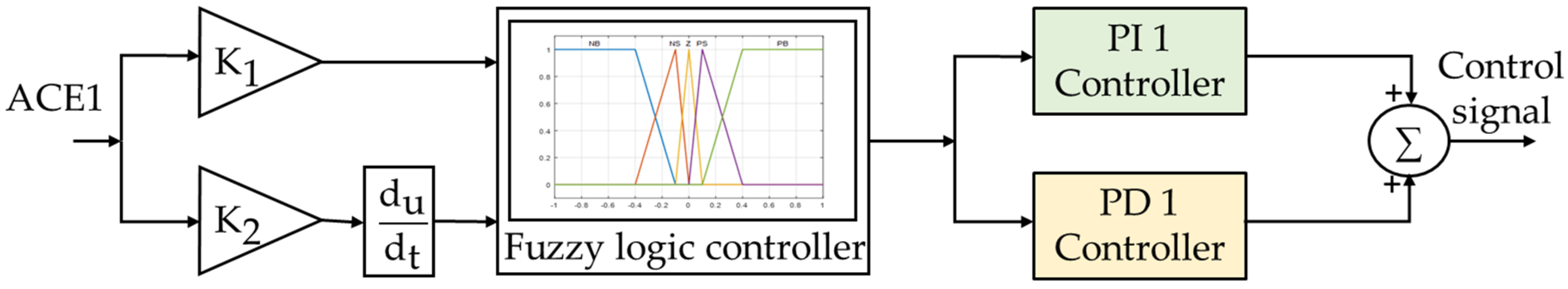
The three novel proposed structures are shown in Figure 16, Figure 17 and Figure 18. Due to the superiority and robustness of the performance of cascading the fraction PI and the fractional PD proposed in [30,31], it is possible to use this idea of cascading to gain further improvement on the performance of the fuzzy controller by proposing a controller that benefits from the advantages of fuzzy control and the merits of the cascading PI and PD controllers. Accordingly, the configuration illustrated in Figure 16 is for the proposed Fuzzy Cascade PI − PD (Fuzzy C PI − PD) employed in area one. This controller has six scaling factor gains. Namely, ${\mathrm{K}}_1$ and ${\mathrm{K}}_2$ are the input gains of the fuzzy controller, ${\mathrm{K}}_{\mathrm{P}11}$ and ${\mathrm{K}}_{\mathrm{I}1}$ are the PI controller gains, and ${\mathrm{K}}_{\mathrm{P}12}$ and ${\mathrm{K}}_{\mathrm{D}1}$ are for the PD controller gains. The identical Fuzzy C PI − PD controller is employed in area two with the following scaling factor gains: ${\mathrm{K}}_3$, ${\mathrm{K}}_4$, ${\mathrm{K}}_{\mathrm{P}21}$, ${\mathrm{K}}_{\mathrm{I}2}$, ${\mathrm{K}}_{\mathrm{P}22}$, and ${\mathrm{K}}_{\mathrm{D}2}$.

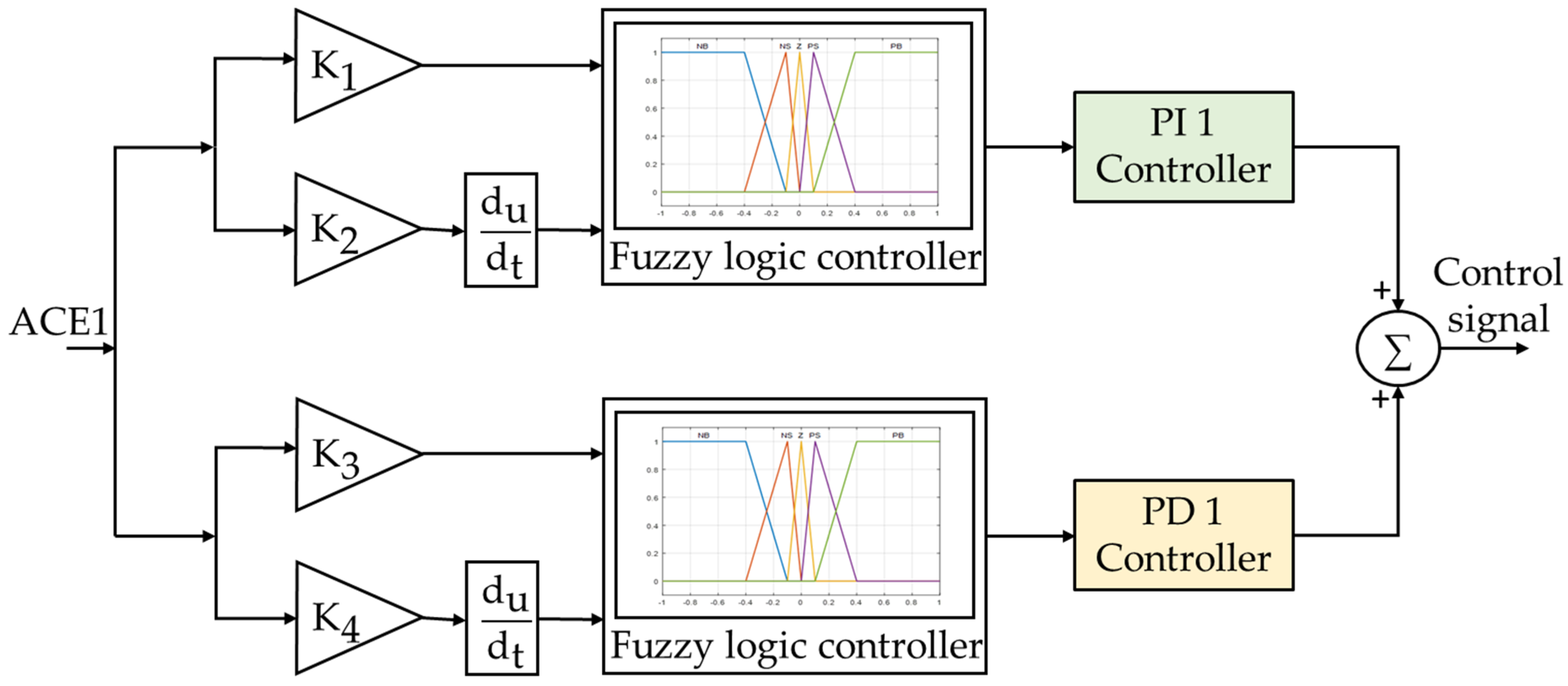
Figure 17 demonstrates the structural diagram of the proposed Fuzzy PI plus Fuzzy PD (Fuzzy PI + Fuzzy PD) controller employed in area one for LFC purposes. As is obvious from the figure, two fuzzy controllers are equipped in each area. This hierarchal configuration should enhance the stability of the system and provide better reliability when any failure occurs in any part of this structure; the other part continues to provide its expected control action.

This controller has eight scaling factor gains. Namely, ${\mathrm{K}}_1$ and ${\mathrm{K}}_2$ are the input gains of the Fuzzy PI controller, ${\mathrm{K}}_{\mathrm{P}11}$ and ${\mathrm{K}}_{\mathrm{I}1}$ are the PI controller gains, ${\mathrm{K}}_3$ and ${\mathrm{K}}_4$ are the input gains of the Fuzzy PD controller, and ${\mathrm{K}}_{\mathrm{P}12}$ and ${\mathrm{K}}_{\mathrm{D}1}$ are for the PD controller gains. The identical Fuzzy PI + Fuzzy PD is employed in area two with the following parameters: ${\mathrm{K}}_5$, ${\mathrm{K}}_6$, ${\mathrm{K}}_{\mathrm{P}21}$, ${\mathrm{K}}_{\mathrm{I}2}$, ${\mathrm{K}}_7$, ${\mathrm{K}}_8, {\mathrm{K}}_{\mathrm{P}22}$, and ${\mathrm{K}}_{\mathrm{D}2}$.

Due to the number of fuzzy rules needed to implement the Fuzzy PI + Fuzzy PD structure in each area [(5 × 5) + (5 × 5) = 50], a longer execution time is required, which may result in slowing down the controller performance; it may be worthwhile to propose another structure that reduces the execution time and guarantees a satisfactory level of reliability. In order to accomplish this, the Fuzzy (PI + PD) shown in Figure 18 is suggested. This structure has less execution time [5 × 5 = 25] and still offers an acceptable range of reliability. This configuration has six scaling factor gains. Namely, ${\mathrm{K}}_1$ and ${\mathrm{K}}_2$ are the input gains of the fuzzy controller, ${\mathrm{K}}_{\mathrm{P}11}$ and ${\mathrm{K}}_{\mathrm{I}1}$ are the PI controller gains, and ${\mathrm{K}}_{\mathrm{P}12}$ and ${\mathrm{K}}_{\mathrm{D}1}$ are for the PD controller gains. A similar Fuzzy C PI − PD controller is employed in area two with the following scaling factor gains: ${\mathrm{K}}_3$, ${\mathrm{K}}_4$, ${\mathrm{K}}_{\mathrm{P}21}$, ${\mathrm{K}}_{\mathrm{I}2}$, ${\mathrm{K}}_{\mathrm{P}22}$, and ${\mathrm{K}}_{\mathrm{D}2}$.

In order to achieve the best possible performance of the proposed fuzzy control configurations, the Bees Algorithm (BA) is used to concurrently find the optimal values of the proposed controllers’ gains by minimising the ITAE of the frequency deviation in both areas and the tie-line power fluctuation. The optimum values of the suggested controllers’ gains are illustrated in

Table 8. The optimum values of the proposed Fuzzy C PI − PD and Fuzzy (PI + PD) controllers obtained by the BA.

Controller	Controller Gains of Area 1						Controller Gains of Area 2
	${\mathbf{K}}_1$	${\mathbf{K}}_2$	${\mathbf{K}}_{\mathbf{P}11}$	${\mathbf{K}}_{\mathbf{I}1}$	${\mathbf{K}}_{\mathbf{P}12}$	${\mathbf{K}}_{\mathbf{D}1}$	${\mathbf{K}}_3$	${\mathbf{K}}_4$	${\mathbf{K}}_{\mathbf{P}21}$	${\mathbf{K}}_{\mathbf{I}2}$	${\mathbf{K}}_{\mathbf{P}22}$	${\mathbf{K}}_{\mathbf{D}2}$
Fuzzy C PI − PD	0.0833	2	2	2	2	2	1.5307	0.0012	1.6472	0.012	0.9902	1.1494
Fuzzy (PI + PD)	0.0594	2	2	2	1.5673	2	2	0.0002	0.001	1.0716	0.4188	0.092

and

Table 9. The optimum Fuzzy PI + Fuzzy PD gains optimized by BA.

Controller	Parameters
Fuzzy PI + Fuzzy PD	Controller gains of area 1
	${\mathrm{K}}_1$	${\mathrm{K}}_2$	${\mathrm{K}}_3$	${\mathrm{K}}_4$	${\mathrm{K}}_{\mathrm{P}11}$	${\mathrm{K}}_{\mathrm{I}1}$	${\mathrm{K}}_{\mathrm{P}12}$	${\mathrm{K}}_{\mathrm{D}1}$
	0.0020	2	0.5981	2	2	2	2	2
	Controller gains of area 2
	${\mathrm{K}}_5$	${\mathrm{K}}_6$	${\mathrm{K}}_7$	${\mathrm{K}}_8$	${\mathrm{K}}_{\mathrm{P}21}$	${\mathrm{K}}_{\mathrm{I}2}$	${\mathrm{K}}_{\mathrm{P}22}$	${\mathrm{K}}_{\mathrm{D}2}$
	2	0.001	0.0004	0.0015	0.3429	0.7511	1.1997	2

. The scaling factors of the proposed fuzzy control configurations are chosen in the limits of [0,1,2].

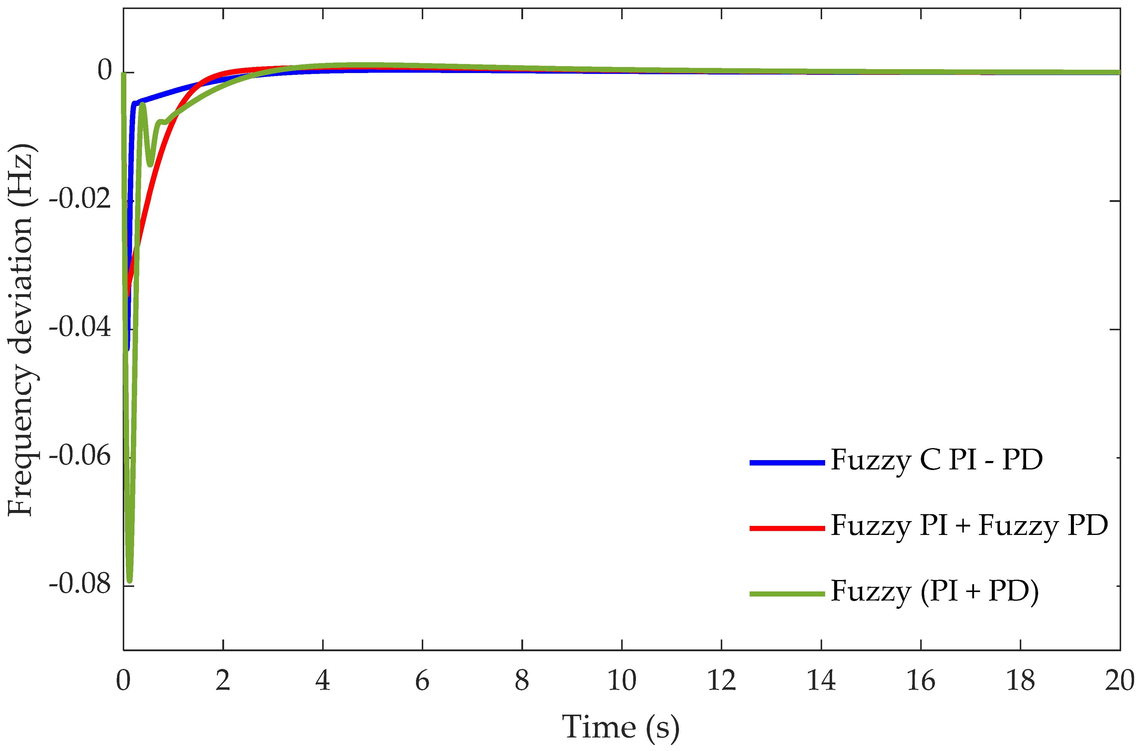
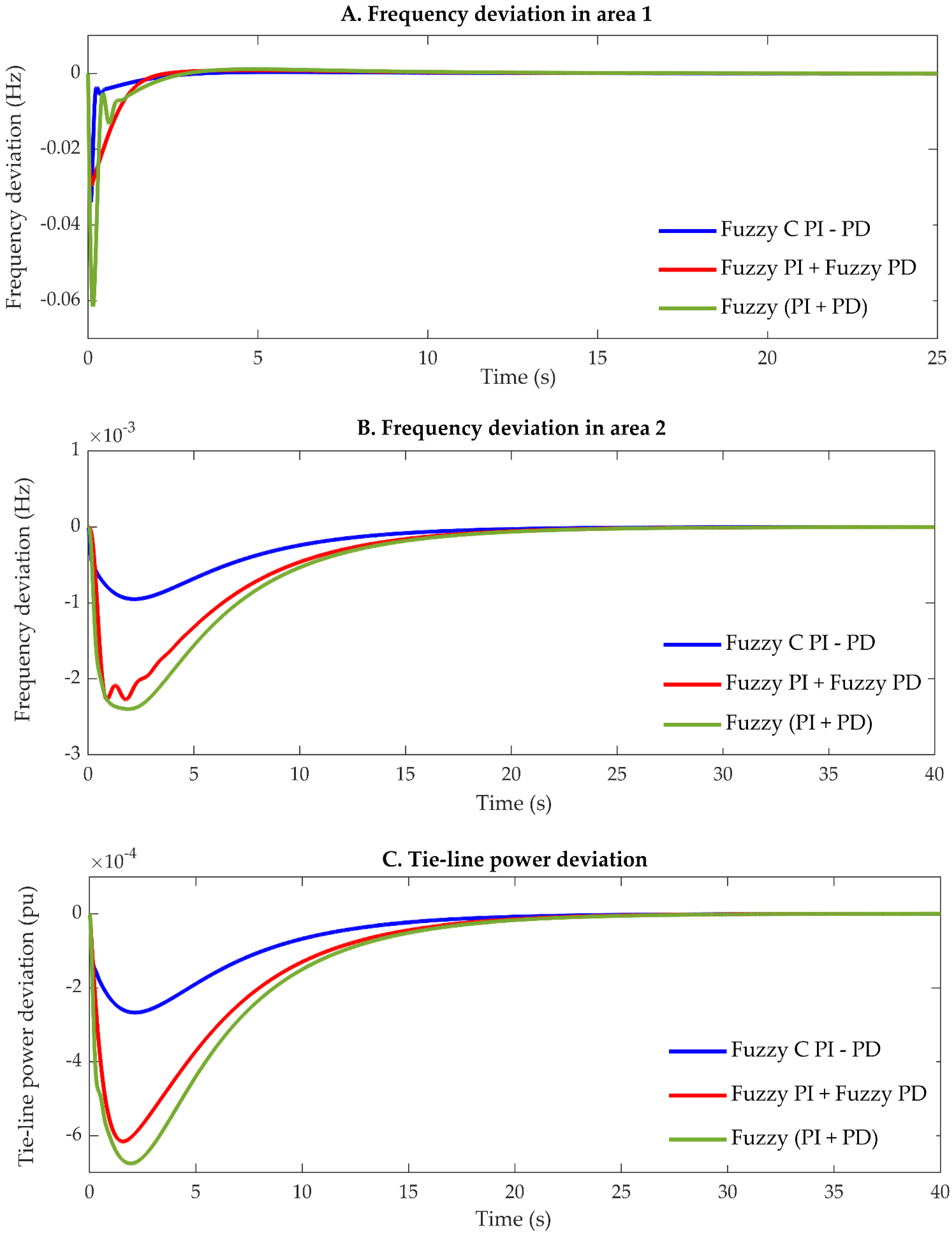
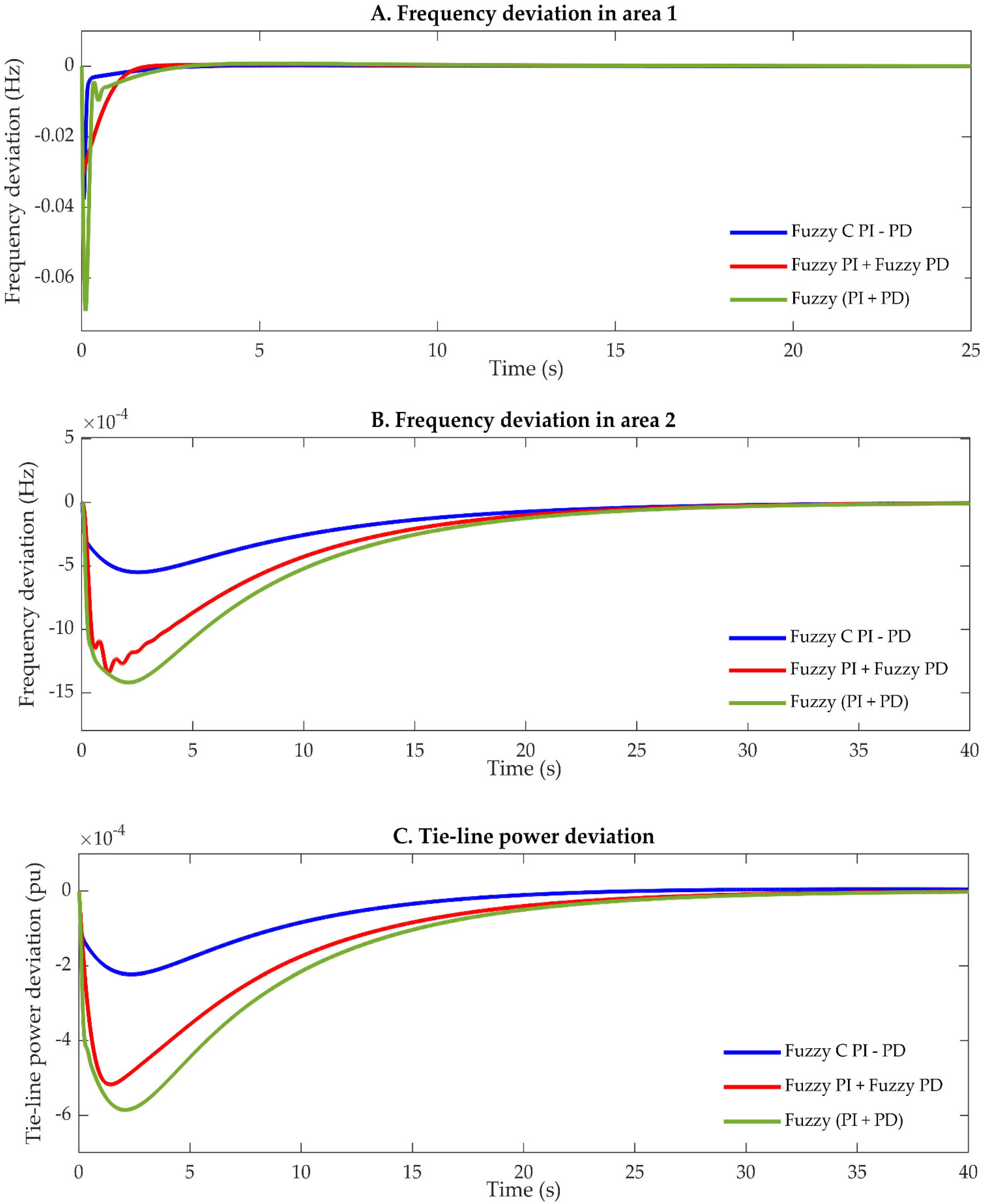
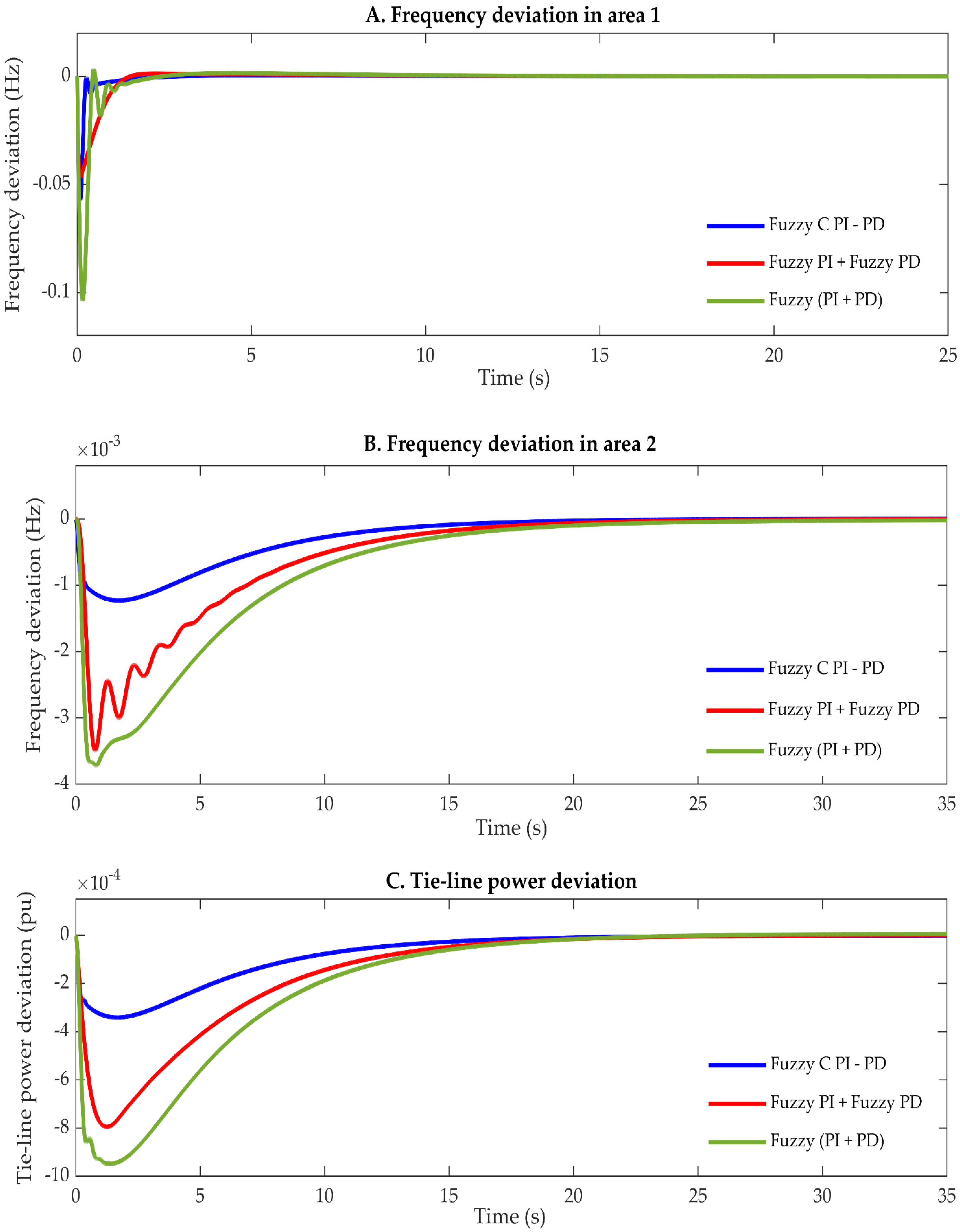
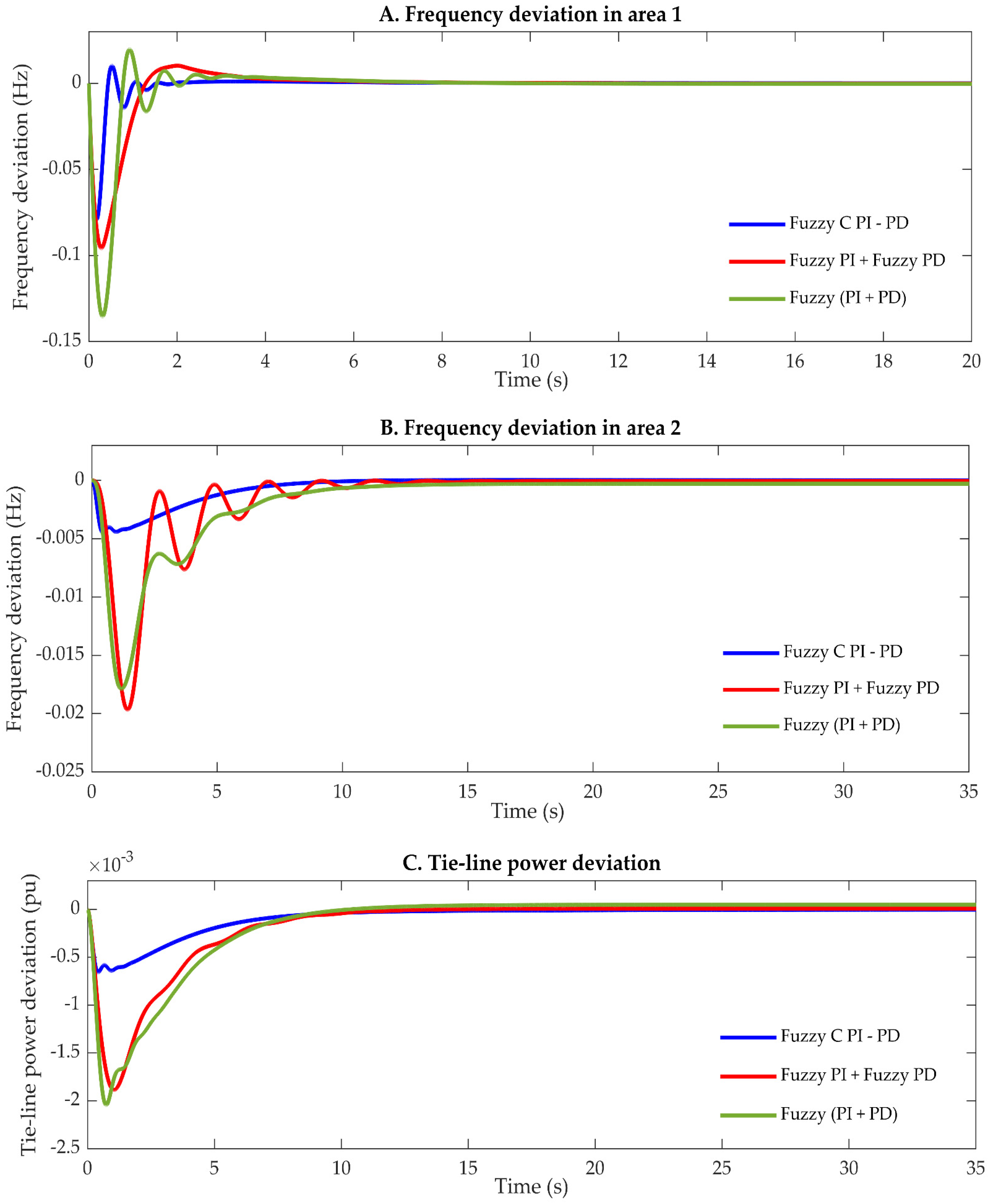
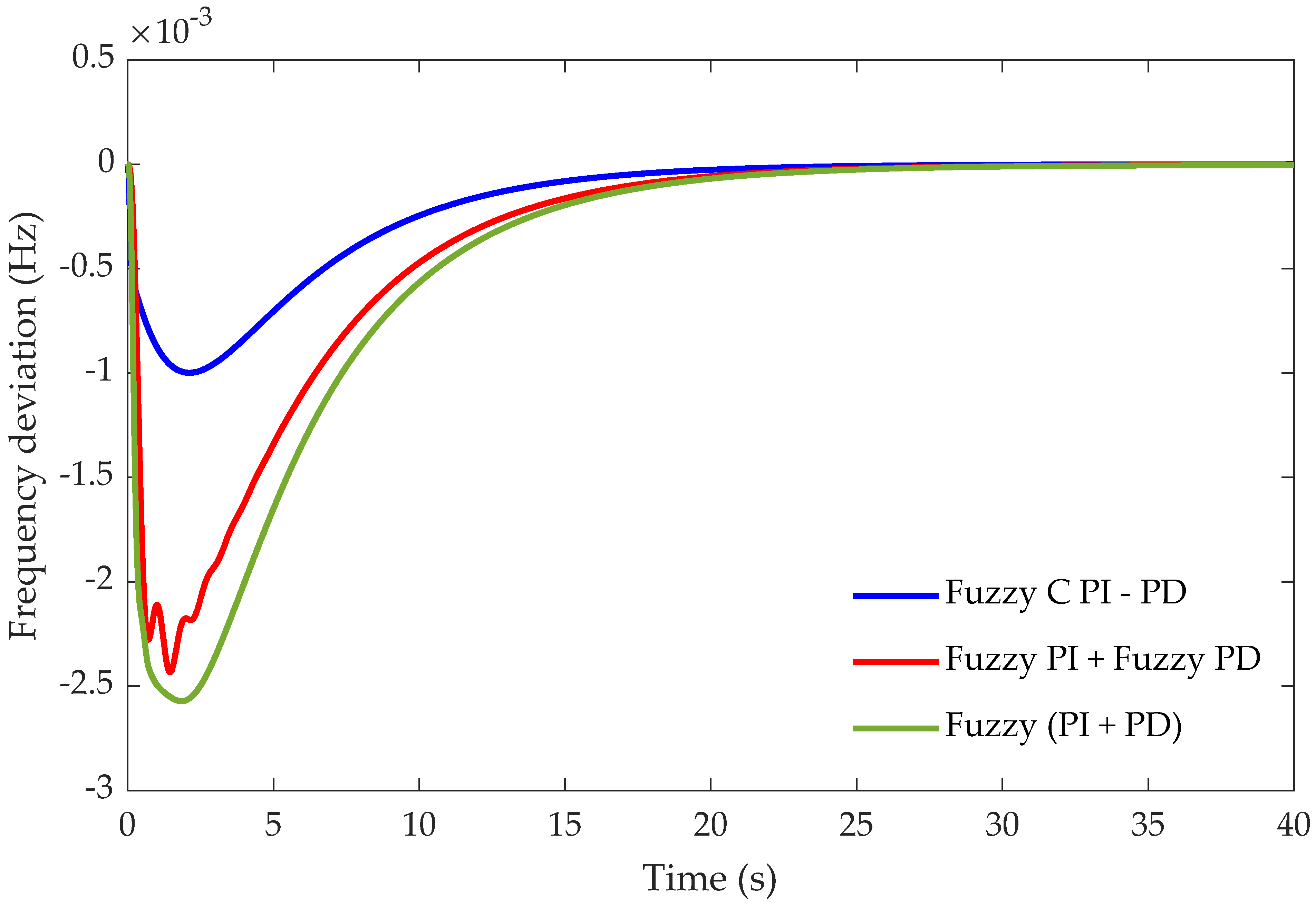
To investigate the performance of the proposed fuzzy control structures, a load disturbance with a magnitude of 0.2 pu is applied in area one at time t = 0. The dynamic response of the system with the proposed controllers employed as the LFCs is demonstrated in Figure 19, Figure 20 and Figure 21. 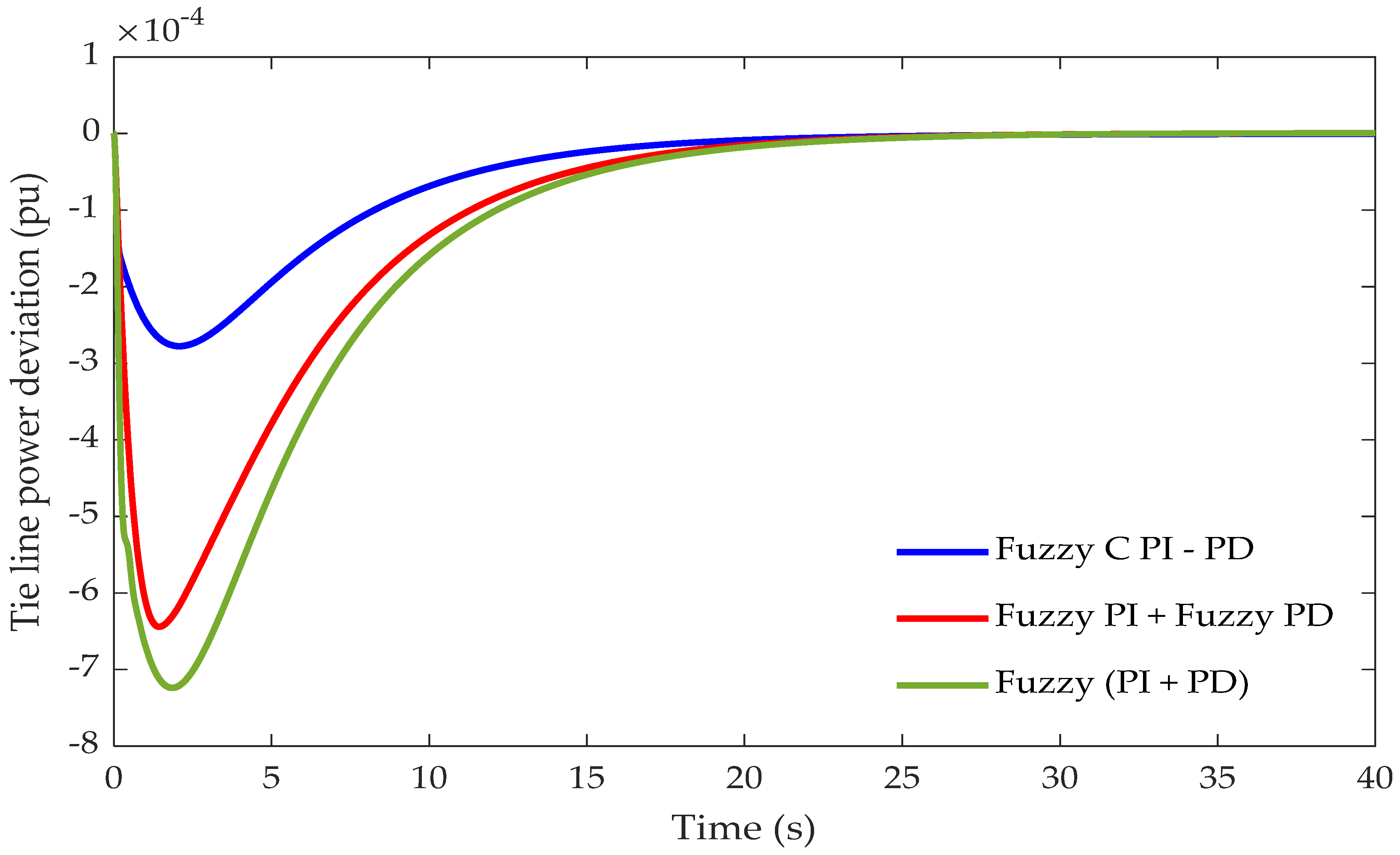The frequency deviation in area one $∆{\mathrm{F}}_1$ in (Hz) is given in Figure 19; the frequency deviation in area two $∆{\mathrm{F}}_2$ in (Hz) is given in Figure 20; and the tie-line power deviation $∆{\mathrm{P}}_{\mathrm{tie}}$ in (pu) is illustrated in Figure 21. Furthermore, the characteristics of the dynamic response represented by the peak undershoot $\left({\mathrm{U}}_{\mathrm{sh}}\right)$, the peak overshoot $\left({\mathrm{O}}_{\mathrm{sh}}\right)$, the settling time $\left({\mathrm{T}}_{\mathrm{s}}\right)$ and the values of the objective function are exemplified in

Table 10. Frequency response performances with different fuzzy control structures tuned by BA.

Controller	Frequency in Area 1			Frequency in Area 2			Tie-Line Power Deviation			ITAE
	${\mathbf{U}}_{\mathbf{sh}}\mathbf{in}\mathbf{Hz}$	${\mathbf{O}}_{\mathbf{sh}}\mathbf{in}\mathbf{Hz}$	${\mathbf{T}}_{\mathbf{s}}\mathbf{in}\mathbf{s}$	${\mathbf{U}}_{\mathbf{sh}}\mathbf{in}\mathbf{Hz}$	${\mathbf{O}}_{\mathbf{sh}}\mathbf{in}\mathbf{Hz}$	${\mathbf{T}}_{\mathbf{s}}\mathbf{in}\mathbf{s}$	${\mathbf{U}}_{\mathbf{sh}}\mathbf{in}\mathbf{pu}$	${\mathbf{O}}_{\mathbf{sh}}\mathbf{in}\mathbf{pu}$	${\mathbf{T}}_{\mathbf{s}}\mathbf{in}\mathbf{s}$
Fuzzy C PI − PD	0.0431	0.00038	2.1873	0.00099	0	21.1703	0.00027	0	21.7522	0.01351
Fuzzy PI + Fuzzy PD	0.0346	0.00089	7.0632	0.0024	0	20.5011	0.00064	0	20.8153	0.02576
Fuzzy (PI + PD)	0.0792	0.00120	2.1384	0.0026	0	21.0681	0.00072	0	21.0885	0.03104

.

The obtained simulation results show that the steady-state responses with the proposed controllers are similar because the frequency variation in both areas and the tie-line power deviation are ceased to zero. However, in terms of the transient response, the least drop in the frequency recorded in area one, as a consequence of the implication of the load disturbance, is −0.0346 Hz; this is achieved based on the proposed Fuzzy PI plus Fuzzy PD structure. Observably, this controller offered the slowest response for $∆{\mathrm{F}}_1$, with a 7.0632 s settling time. Furthermore, a negligible overshoot is observed in the dynamic response obtained based on the three suggested controllers. Regarding the drop in the frequency in area two, the proposed structures have provided satisfactory responses with a slight superiority of the Fuzzy C PI − PD over the other two structures. The tie-line power deviation of the system is illustrated in Figure 21, where the supremacy of the Fuzzy C PI − PD over the other controllers is observed. Moreover, the value of the ITAE is the smallest for the Fuzzy C PI − PD tuned by the BA as compared with the other structures tuned by the same algorithm.

Based on the simulation results provided in Figure 19, Figure 20 and Figure 21 and Table 10, it is evidenced that the proposed fuzzy configurations are serving as effective solutions for the issue of LFC as they provide different advantages, such as fast response with neglectable overshoot and zero steady-state error. Importantly, based on their structures, these controllers offer a wide range of reliability.

7. Robustness Investigation of Fuzzy Cascade PI − PD, Fuzzy PI + PD, and Fuzzy PI plus Fuzzy PD

The investigated two-area power system has several parameters that may vary due to different operating conditions. This variation influences the stability of the system. For example, the increase in the governor time constant (Tg) results in an increase in the frequency deviation, while decreasing the damping ratio (D) may lead to increasing the frequency deviation of the system, which may bring about a possibility of system instability. Moreover, increasing the inertia time constant (H) can slow down the system. Therefore, the LFC system should have the required control action towards the parametric uncertainties of the controlled system and provide an acceptable level of robustness.

Accordingly, to assess the robustness of the proposed fuzzy control configurations tuned by the BA equipped as an LFC system in the dual-area power system, thirteen scenarios are assumed for the parametric uncertainties of the testbed system, as given in

Table 11. Investigated scenarios of system parametric variations.

Case	Parameters	Nominal Values		Variation Range	New Values
Number		Area 1	Area 2		Area 1	Area 2
Case 1	H	5	4	+50%	7.5	6
Case 2	H	5	4	−50%	2.5	2
Case 3	Tt	0.5	0.6	+50%	0.75	0.9
Case 4	Tt	0.5	0.6	−50%	0.25	0.3
Case 5	B	20.6	16.9	+50%	30.9	25.35
Case 6	B	20.6	16.9	−50%	10.3	8.45
Case 7	D	0.6	0.9	+50%	0.9	1.35
Case 8	D	0.6	0.9	−50%	0.3	0.45
Case 9	Tg	0.2	0.3	+50%	0.3	0.45
Case 10	Tg	0.2	0.3	−50%	0.1	0.15
Case 11	R	0.05	0.0625	+50%	0.075	0.0937
Case 12	R	0.05	0.0625	−50%	0.025	0.0312
Case 13	B	20.6	16.9	−50%	10.3	8.45
	H	5	4	+50%	7.5	6
	R	0.05	0.0625	+50%	0.075	0.0937
	D	0.6	0.9	−50%	0.3	0.45
	Tt	0.5	0.6	+50%	0.75	0.9
	Tg	0.2	0.3	+50%	0.3	0.45

. This assessment begins with individually varying each parameter in the system by (+ and −) 50% from their nominal values. As is understood, changing the parameters from their nominal values may have a positive impact on the overall system stability. Therefore, in order to make this analysis more credible, all the parameters are simultaneously varied from their nominal values. Accordingly, in case thirteen, we consider the negative impact of each parameter of uncertainty and change them simultaneously. This guarantees the assessment of the robustness in the worst scenario that the system may experience during the working time. An SLP of 0.2 pu is applied in area one to examine the effect of the system parametric uncertainties on the behavior of the Fuzzy C PI − PD, Fuzzy PI + PD, and Fuzzy PI plus Fuzzy PD; a comparative study is given based on the obtained results. Fuzzy control robustness analysis can also be carried out in different ways as investigated in [32,33,34].

From case 1 to case 12 in Table 11, only a single parameter is changed at a time by +50% and −50% from its nominal value. In case thirteen, the parameters Tg, Tt, H, and R in both areas are varied by 50%, while the parameters B and D are varied by −50%. The dynamic response of the system with the proposed controllers under parametric uncertainty conditions is demonstrated in Figure 22, Figure 23, Figure 24, Figure 25, Figure 26, Figure 27, Figure 28, Figure 29, Figure 30, Figure 31, Figure 32, Figure 33 and Figure 34. Moreover, the characteristics of the transient response are depicted in

Table 12. Dynamic response of the system under different parametric uncertainties scenarios with different controllers.

Case No	Controller	Frequency in Area 1			Frequency in Area 2			Tie-Line Power Deviation
		${\mathbf{U}}_{\mathbf{sh}}\mathbf{in}\mathbf{Hz}$	${\mathbf{O}}_{\mathbf{sh}}\mathbf{in}\mathbf{Hz}$	${\mathbf{T}}_{\mathbf{s}}\mathbf{in}\mathbf{s}$	${\mathbf{U}}_{\mathbf{sh}}\mathbf{in}\mathbf{Hz}$	${\mathbf{O}}_{\mathbf{sh}}\mathbf{in}\mathbf{Hz}$	${\mathbf{T}}_{\mathbf{s}}\mathbf{in}\mathbf{s}$	${\mathbf{U}}_{\mathbf{sh}}\mathbf{in}\mathbf{pu}$	${\mathbf{O}}_{\mathbf{sh}}\mathbf{in}\mathbf{pu}$	${\mathbf{T}}_{\mathbf{s}}\mathbf{in}\mathbf{s}$
Case 1	Fuzzy C PI − PD	−0.0339	0.00037	2.380	−0.00095	0	21.4962	−0.00026	0	21.697
	Fuzzy PI + Fuzzy PD	−0.0297	0.00087	7.768	−0.0023	0	20.7037	−0.00061	0	20.895
	Fuzzy (PI + PD)	−0.0615	0.0011	2.305	−0.0024	0	21.107	−0.00067	0	21.117
Case 2	Fuzzy C PI − PD	−0.0695	0.00044	1.713	−0.0012	0	20.714	−0.00032	0	21.688
	Fuzzy PI + Fuzzy PD	−0.0579	0.0012	2.455	−0.0032	0	19.835	−0.00080	0	20.300
	Fuzzy (PI + PD)	−0.1268	0.0010	1.765	−0.0030	0	20.947	−0.00085	0	20.972
Case 3	Fuzzy C PI − PD	−0.0585	0.0005	1.5501	−0.0013	0	20.157	−0.00036	0	21.1190
	Fuzzy PI + Fuzzy PD	−0.0486	0.0023	6.0375	−0.0039	0	18.896	−0.00090	0	19.8623
	Fuzzy (PI + PD)	−0.1074	0.0017	1.5144	−0.0042	0	19.826	−0.0010	0	20.4457
Case 4	Fuzzy C PI − PD	−0.0260	0.00032	2.955	−0.00082	0	22.077	−0.00023	0	22.223
	Fuzzy PI + Fuzzy PD	−0.0220	0.00075	9.0899	−0.0018	0	21.720	−0.00049	0	21.757
	Fuzzy (PI + PD)	−0.0483	0.00092	2.851	−0.0019	0	21.611	−0.00054	0	21.633
Case 5	Fuzzy C PI − PD	−0.0377	0.00025	2.0857	−0.00054	0	31.659	−0.00022	0	25.188
	Fuzzy PI + Fuzzy PD	−0.0307	0.00056	1.6032	−0.0013	0	27.7717	−0.00051	0	28.1434
	Fuzzy (PI + PD)	−0.0693	0.00077	2.1015	−0.0014	0	28.6358	−0.00058	0	28.660
Case 6	Fuzzy C PI − PD	−0.0577	0.00074	2.1637	−0.0028	0	19.4344	−0.00040	0	26.209
	Fuzzy PI + Fuzzy PD	−0.0546	0.0018	6.3768	−0.0080	0	11.6084	−0.00099	0	12.1848
	Fuzzy (PI + PD)	−0.1029	0.0021	4.8285	−0.0074	0	11.8962	−0.0010	0	12.1313
Case 7	Fuzzy C PI − PD	−0.0430	0.00038	2.1892	−0.00099	0	20.927	−0.00027	0	22.192
	Fuzzy PI + Fuzzy PD	−0.0346	0.00098	7.0758	−0.0024	0	20.531	−0.00064	0	20.837
	Fuzzy (PI + PD)	−0.0790	0.0012	2.141	−0.0026	0	21.084	−0.00072	0	21.104
Case 8	Fuzzy C PI − PD	−0.0431	0.00038	2.1854	−0.0010	0	21.418	−0.00027	0	21.325
	Fuzzy PI + Fuzzy PD	−0.0347	0.00089	7.0507	−0.0024	0	20.470	−0.00064	0	20.792
	Fuzzy (PI + PD)	−0.0794	0.0012	2.1359	−0.0026	0	20.052	−0.00072	0	21.072
Case 9	Fuzzy C PI − PD	−0.0573	0.00047	1.724	−0.0012	0	20.633	−0.00034	0	21.414
	Fuzzy PI + Fuzzy PD	−0.0468	0.0013	5.788	−0.0035	0	19.235	−0.00079	0	20.257
	Fuzzy (PI + PD)	−0.1038	0.0032	1.7013	−0.0037	0	20.298	−0.00094	0	20.738
Case 10	Fuzzy C PI − PD	−0.0267	0.00034	2.7138	−0.00086	0	21.6312	−0.00024	0	21.995
	Fuzzy PI + Fuzzy PD	−0.0224	0.0080	8.9968	−0.0019	0	21.285	−0.00053	0	21.362
	Fuzzy (PI + PD)	−0.0507	0.00098	2.5984	−0.0021	0	21.339	−0.00057	0	21.378
Case 11	Fuzzy C PI − PD	−0.0431	0.00038	2.1736	−0.001	0	24.738	−0.00027	0	17.791
	Fuzzy PI + Fuzzy PD	−0.0346	0.0089	6.953	−0.0025	0	20.2308	−0.00064	0	20.496
	Fuzzy (PI + PD)	−0.0792	0.0012	2.1284	−0.0026	0	20.848	−0.00072	0	20.863
Case 12	Fuzzy C PI − PD	−0.0430	0.00041	2.212	−0.00095	0	14.328	−0.00027	0	32.2229
	Fuzzy PI + Fuzzy PD	−0.0346	0.00089	7.3773	−0.0023	0	21.268	−0.00063	0	21.7101
	Fuzzy (PI + PD)	−0.0790	0.0011	2.1689	−0.0024	0	21.693	−0.00071	0	21.7307
Case 13	Fuzzy C PI − PD	−0.0791	0.01027	1.435	−0.0045	0.00004	9.9188	−0.00065	0	14.922
	Fuzzy PI + Fuzzy PD	−0.0958	0.0103	5.1487	−0.0197	0	10.577	−0.00190	0.000007	10.393
	Fuzzy (PI + PD)	−0.1354	0.020	4.9656	−0.0179	0	10.1364	−0.0020	0.000047	10.681

Values that represent the best characteristics are indicated in bold.

.

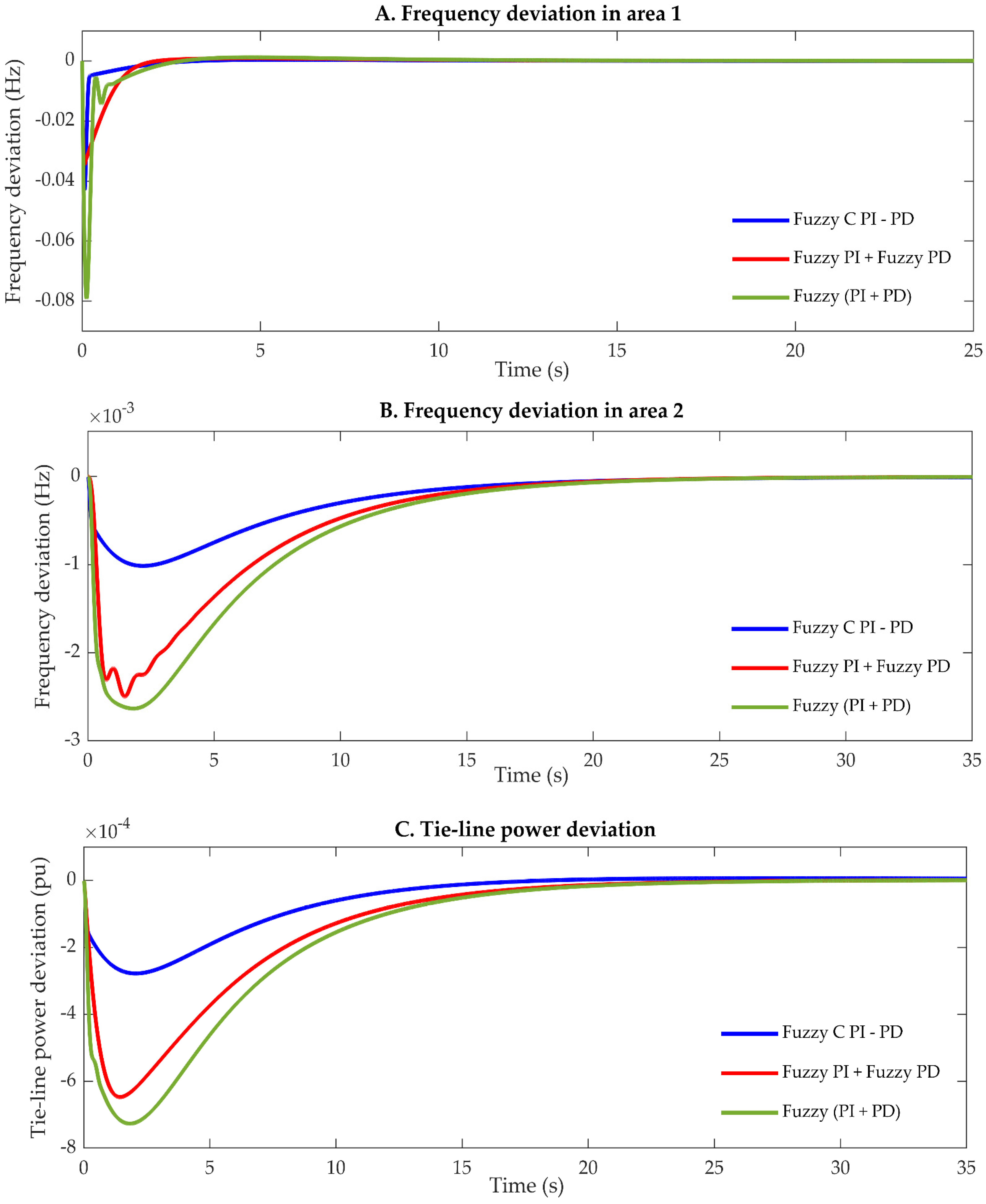
Figure 22 illustrates the dynamic behavior of the testbed system based on the proposed fuzzy control structures under parametric uncertainty case 1, where the inertia time constants in both areas are altered by +50% from their nominal values. It is noted that the increase in the time inertia has slowed the response of the system. For example, the settling time of the frequency in area one has increased from 2.1873 s, 7.0632 s, and 2.1384 s to 2.380 s, 7.768 s, and 2.305 s based on Fuzzy C PI − PD, Fuzzy PI plus Fuzzy PD, and Fuzzy PI + PD, respectively. The settling time of $∆{\mathrm{F}}_2$ and $∆{\mathrm{P}}_{\mathrm{tie}}$ follow the same pattern, where a slight increase is observed. Moreover, it is concluded that the increase in the inertia time constant has led to a slight decrease in the drop of the frequency in both areas. Conversely, the decrease in the inertia time constant which is considered in case 2 brings about a further drop in the frequency and the tie-line power deviation in the system. Moreover, it leads to a slight improvement in terms of the settling time in $∆{\mathrm{F}}_1$, $∆{\mathrm{F}}_2$, and $∆{\mathrm{P}}_{\mathrm{tie}}$. 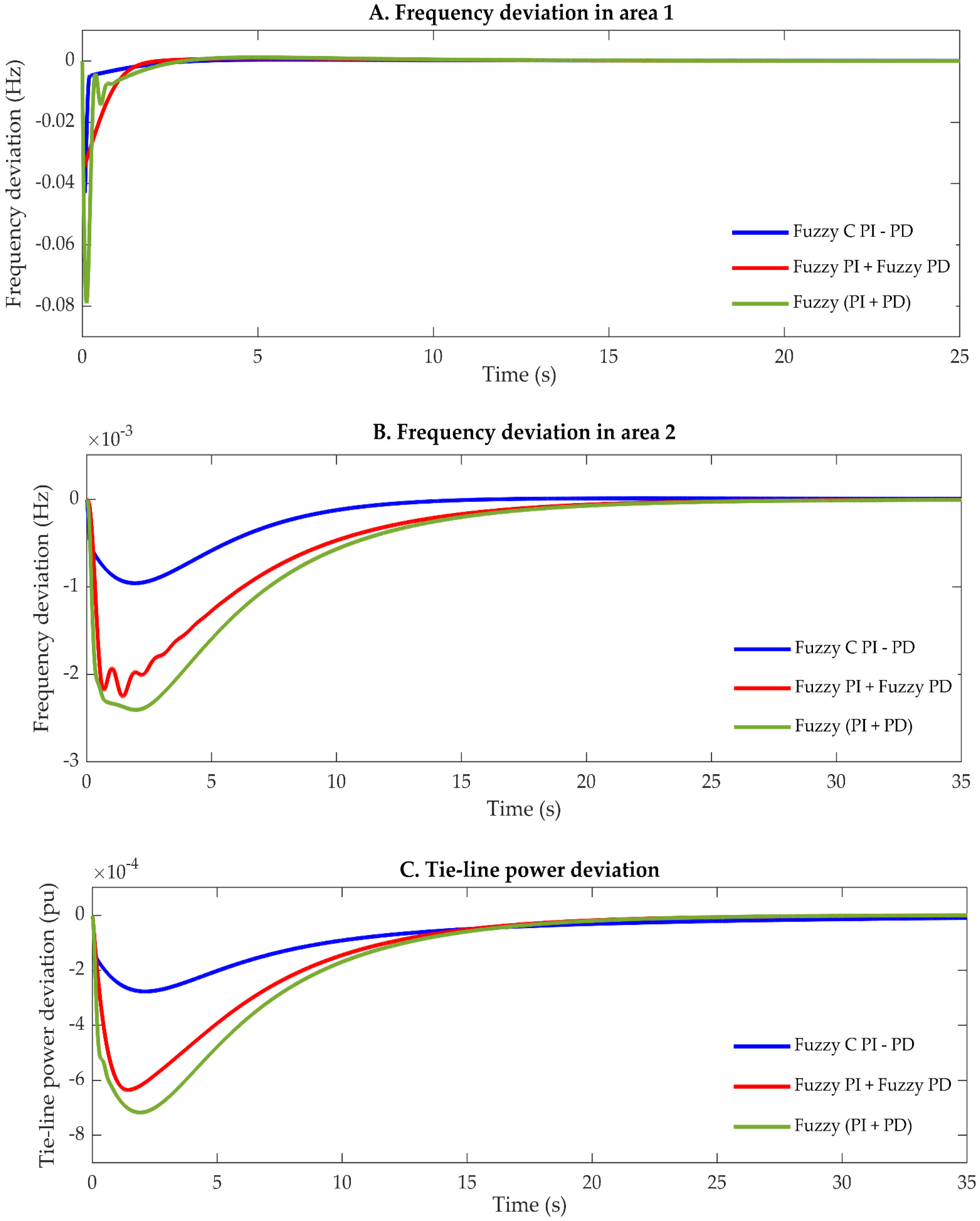Figure 23 shows the dynamic performance of the system based on the proposed controllers under parametric uncertainty case 2.

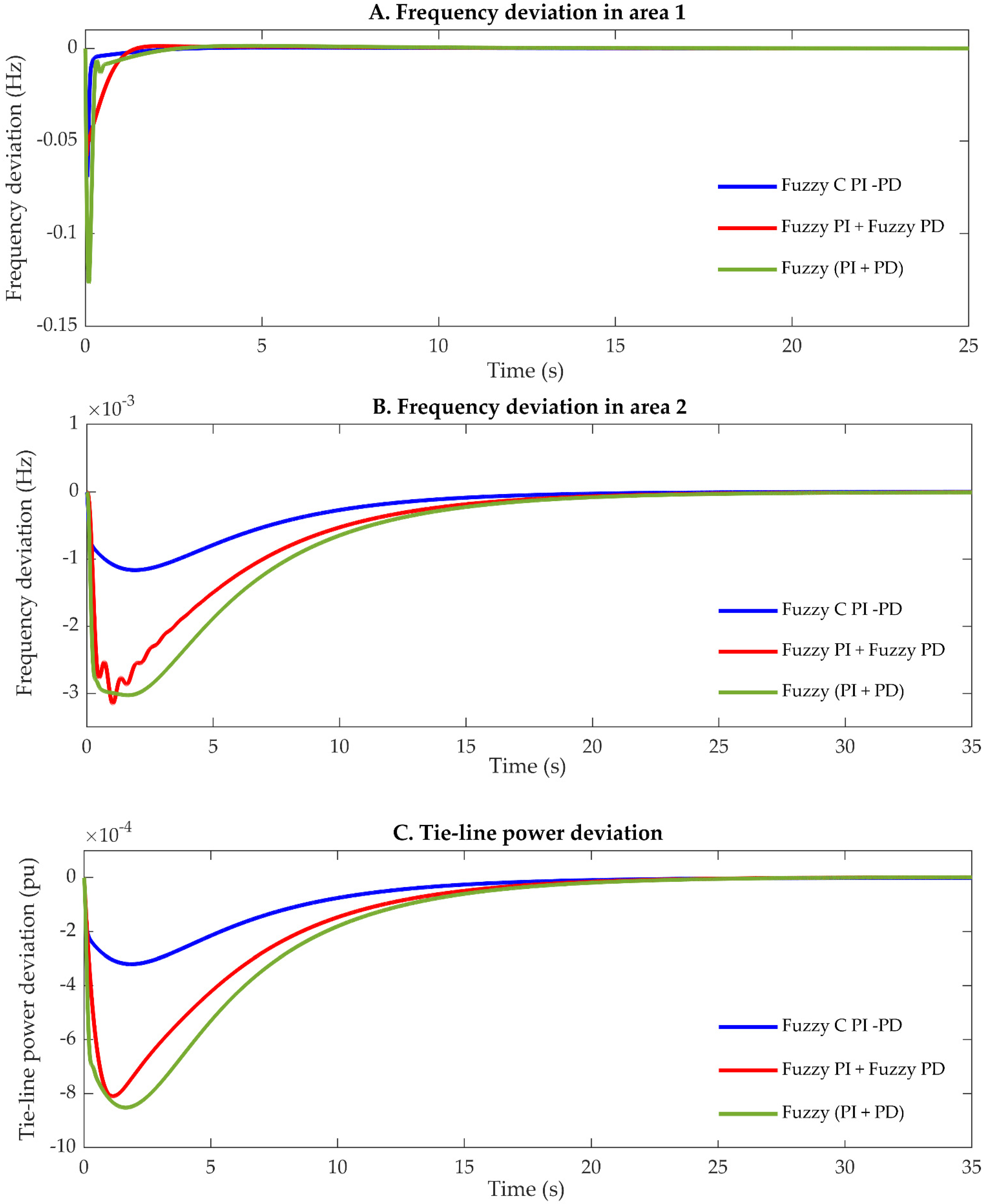
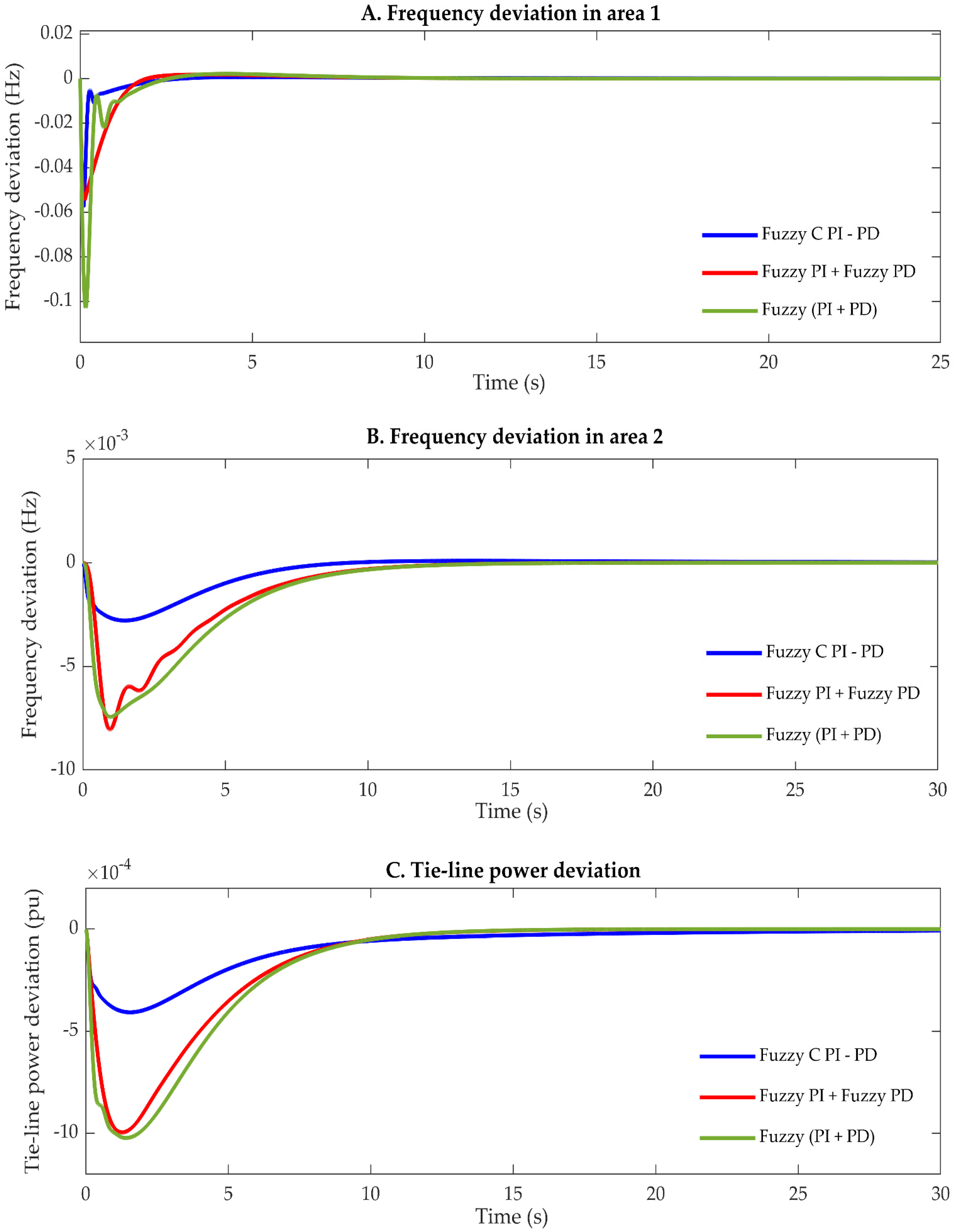
The impact of uncertainty in the turbine time constant is investigated in case 3 and case 4. Figure 24 demonstrates the dynamic performance of the testbed system based on the proposed fuzzy configurations under parametric uncertainty case 3, where the turbine time constants in both areas are varied by +50% from their nominal values. From Figure 24 and Table 12, it is noticed that as a consequence of increasing the turbine time constants within the system, the drop in the frequency in area one ($∆{\mathrm{F}}_1$) has jumped from −0.0431 Hz, −0.0346 Hz, and −0.0792 Hz to −0.0585 Hz, −0.0486 Hz, and −0.1074 Hz. While the drop of the frequency in area two ($∆{\mathrm{F}}_2$) increased from −0.00099 Hz, −0.0024 Hz, and −0.0026 Hz to −0.0013 Hz, −0.0039 Hz, and −0.0042 Hz, based on Fuzzy C PI − PD, Fuzzy PI plus Fuzzy PD, and Fuzzy PI + PD, respectively. It is also obvious that due to the increase of the turbine time constant, the settling time of the $∆{\mathrm{F}}_1$, $∆{\mathrm{F}}_2$, and $∆{\mathrm{P}}_{\mathrm{tie}}$ has slightly decreased. In contrast, from Figure 25, the decline in the turbine time constant brings about a decrease in the frequency deviation and slightly slows the system.

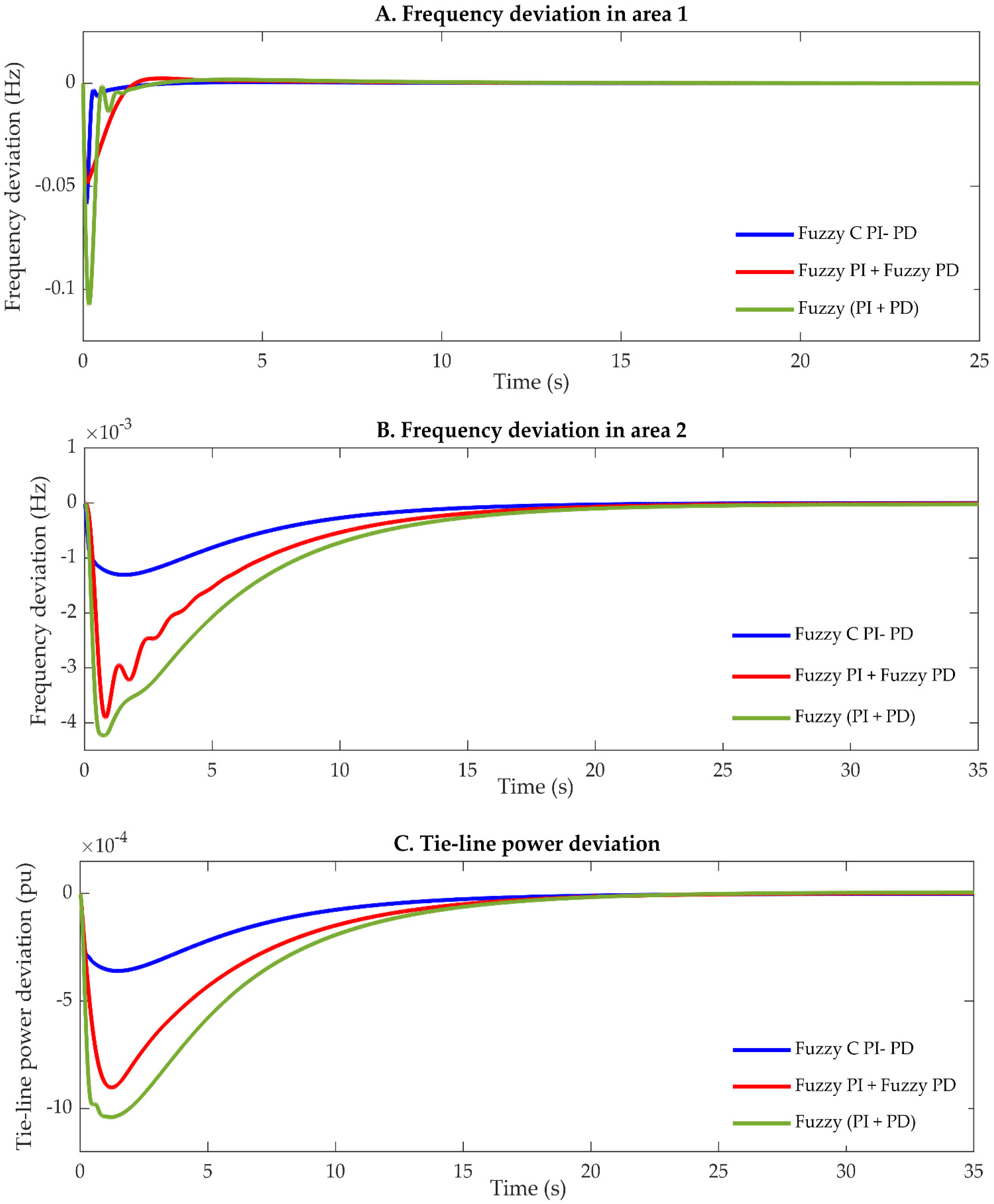
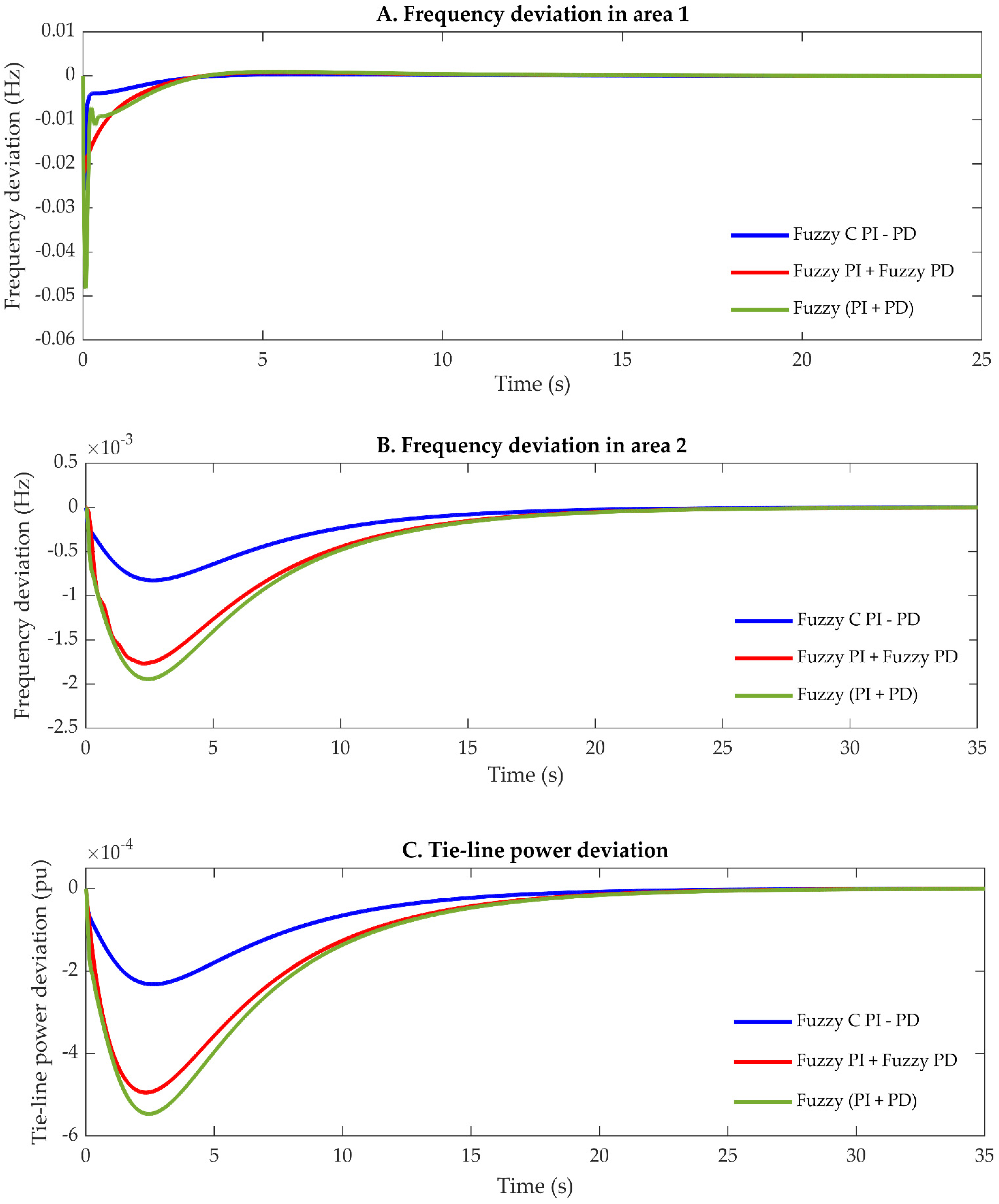
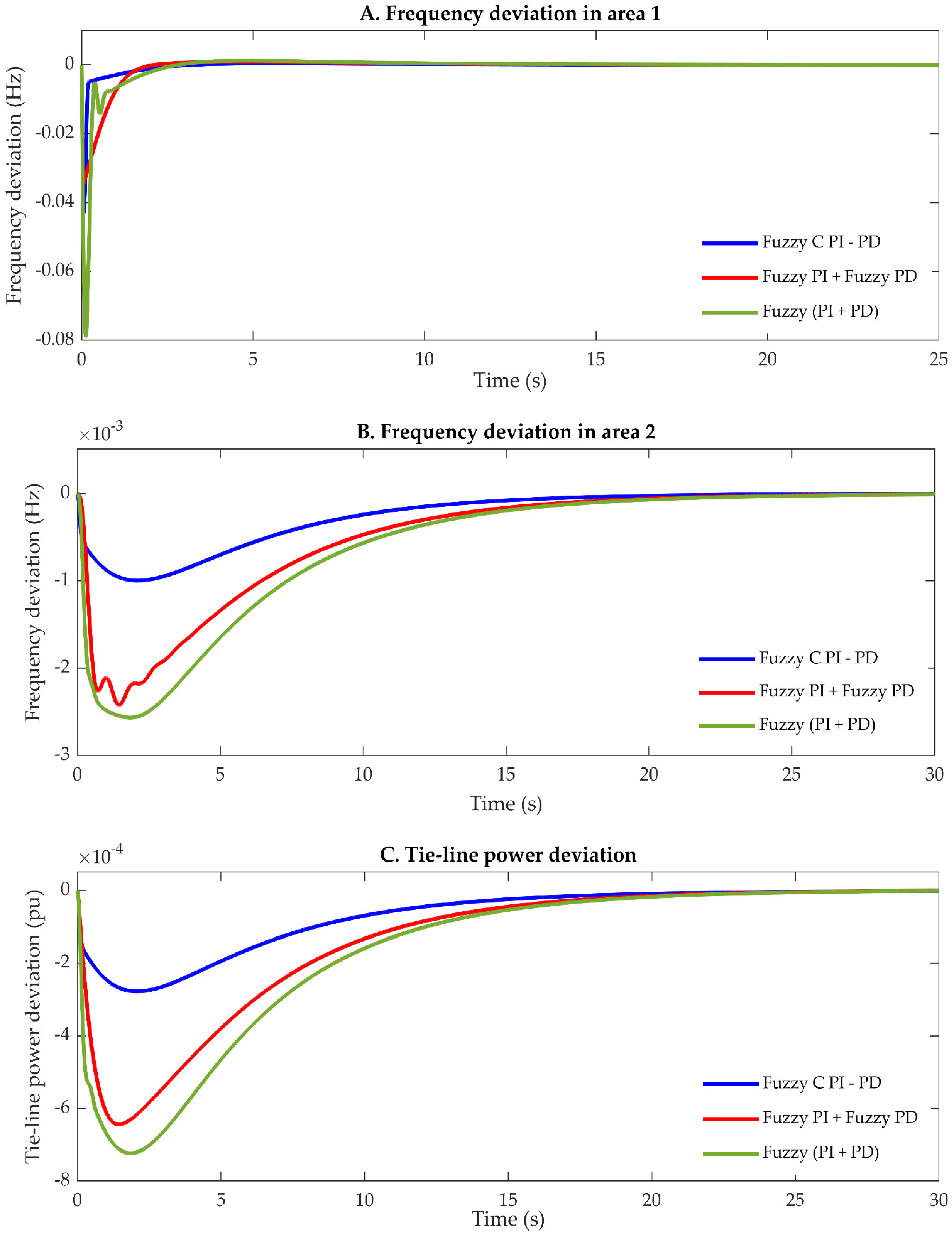
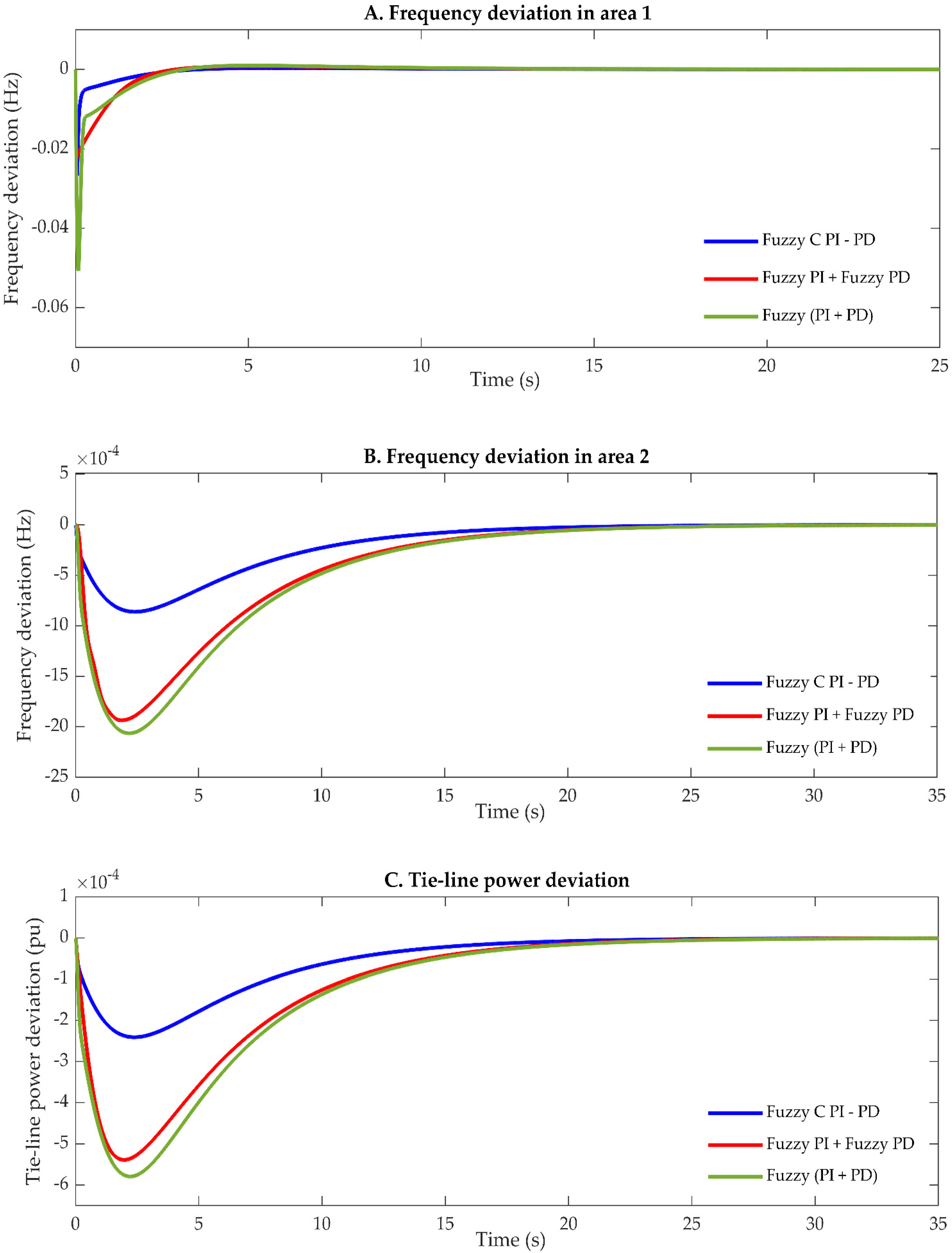
Figure 26 indicates the dynamic response of the system under parametric uncertainty case 5. In this case, the frequency bias in both areas is altered by +50%. It is noticed that the increase in frequency bias has marginally improved the dynamic response in terms of the drop in the frequency, where the maximum undershoot of the frequency in area one ($∆{\mathrm{F}}_1$) has decreased from −0.0431 Hz, −0.0346 Hz, and −0.0792 Hz to −0.0377 Hz, −0.0307 Hz, and −0.0693 Hz, while the drop of the frequency in area two ($∆{\mathrm{F}}_2$) declined from −0.00099 Hz, −0.0024 Hz, and −0.0026 Hz to −0.00054 Hz, −0.0013 Hz, and −0.0014 Hz, based on Fuzzy C PI − PD, Fuzzy PI plus Fuzzy PD, and Fuzzy PI + PD, respectively. With regard to the influence of decreasing the frequency bias on the stability of the power systems which are considered in case 6 and illustrated in Figure 27, it is obvious that the decrease in the frequency bias has slightly worsened the dynamic response of the system in terms of the frequency variation, where it is noted that the maximum undershoot of the frequency in area one has increased from −0.0431 Hz, −0.0346 Hz, and −0.0792 Hz to −0.0577 Hz, −0.0546 Hz, and −0.1029 Hz, while the drop of the frequency in area two ($∆{\mathrm{F}}_2$) increased from −0.00099 Hz, −0.0024 Hz, and −0.0026 Hz to −0.0028 Hz, −0.0080 Hz, and −0.0074 Hz, based on Fuzzy C PI − PD, Fuzzy PI plus Fuzzy PD, and Fuzzy PI + PD, respectively.

The influence of uncertainty in the damping constant (D) is investigated in cases 7 and 8. Figure 28 and Figure 29 demonstrate the dynamic performance of the testbed system based on the proposed fuzzy structures under the parametric uncertainty conditions of cases 7 and 8, where the damping constants (D) in both areas are varied by +50% and −50% from their nominal values. Due to the change in this parameter, a negligible change in the dynamic performance of the system is observed based on these cases as compared with the results obtained using the nominal conditions.

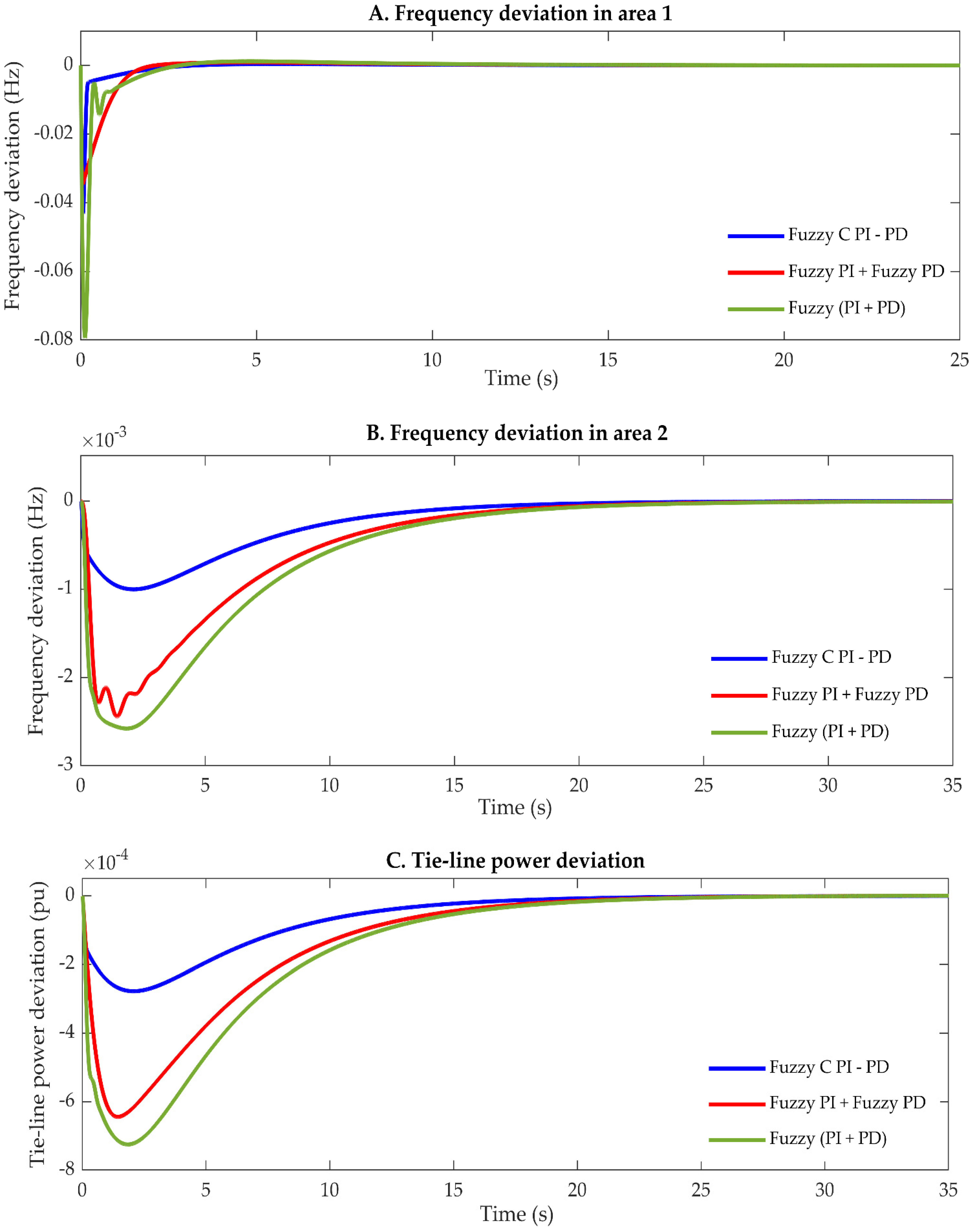
The uncertainty in the governor time constant (Tg) has a similar impact of uncertainty as the turbine time constant on the stability of the system in terms of frequency variation and the speed of the response. Figure 30 reveals the dynamic performance of the dual-area power system when the proposed fuzzy structures are employed as LFCs in the system with the consideration of parametric uncertainty case 9, where the governor time constants in both areas are varied by +50% from their nominal values. As a result of uncertainty in the governor time constants within the system, the drop in the frequency in area one ($∆{\mathrm{F}}_1$) has incremented from −0.0431 Hz, −0.0346 Hz, and −0.0792 Hz to −0.0573 Hz, −0.0468 Hz, and −0.1038 Hz, while the drop in the frequency in area two ($∆{\mathrm{F}}_2$) increased from −0.00099 Hz, −0.0024 Hz, and −0.0026 Hz to −0.0012 Hz, −0.0035 Hz, and −0.0037 Hz, based on Fuzzy C PI − PD, Fuzzy PI + PD, and Fuzzy PI plus Fuzzy PD, respectively. Moreover, the settling time of $∆{\mathrm{F}}_1$ decreased from 2.1873 s, 7.0632 s, and 2.1384 s to 1.724 s, 5.788 s, and 1.7013 s, based on Fuzzy C PI − PD, Fuzzy PI plus Fuzzy PD, and Fuzzy PI + PD, respectively. The dynamic response of the system under parametric uncertainty case 10 is illustrated in Figure 31. In this case of robustness analysis, the governor time constants in both areas are varied by −50% from their nominal values. The results obtained based on case 10 revealed that the decrease in the governor time constant results in a clear decrease in the frequency variation and tie-line power deviation.

Figure 32 and Figure 33 show the dynamic response of the testbed system for parametric uncertainties in case 11 and case 12, respectively. In case 11, the regulation constant in both areas is varied by +50% while it is altered by −50% in case 12. The obtained results based on cases 12 and 13 demonstrate that the uncertainty in the regulation constant has a small impact on the system stability when the proposed fuzzy controllers are equipped in the system for load frequency control.

The worst drop in frequency in both areas ($∆{\mathrm{F}}_1$) and ($∆{\mathrm{F}}_2$), as well as in the tie-line power deviation ($∆{\mathrm{P}}_{\mathrm{tie}}$), is recorded based on the results obtained from case 13 of the robustness analysis, as shown in Figure 34, where the drop of the frequency in area one has increased from −0.0431 Hz, −0.0346 Hz, and −0.0792 Hz to −0.0791 Hz, −0.0958 Hz, and −0.1354 Hz. The drop of the frequency in area two increased from −0.00099 Hz, −0.0024 Hz, and −0.0026 Hz to −0.0045 Hz, −0.0197 Hz, and −0.0179 Hz, whilst the maximum overshoot of the tie-line power deviation increased from −0.00027 pu, −0.00064 pu, and −0.00072 pu to −0.00065 pu, −0.0019 pu, and −0.0020 pu, based on Fuzzy C PI − PD, Fuzzy PI plus Fuzzy PD, and Fuzzy PI + PD, respectively.

From Figure 22, Figure 23, Figure 24, Figure 25, Figure 26, Figure 27, Figure 28, Figure 29, Figure 30, Figure 31, Figure 32, Figure 33 and Figure 34 and Table 12, despite the wide range of parametric uncertainties of the investigated two-area system in the thirteen considered scenarios, the implementation of the three fuzzy control configurations tuned by the BA suggested in this study has shown an excellent level of robustness which preserved the stability of the system within acceptable limits. Furthermore, although there is the similarity of the performance of the proposed configurations, it is obvious that the proposed Fuzzy C PI − PD and Fuzzy PI plus Fuzzy PD have outperformed the Fuzzy PI + PD in all aspects.

8. Conclusions

This study proposes a design and implementation of a Fuzzy PID with a filtered derivative action (Fuzzy PIDF) for the LFC to enhance the stability of a dual-area interconnected power system. The TLBO, PSO, and BA optimization tools were utilized to obtain the optimum values of the proposed controller parameters by reducing the ITAE objective function. A disturbance of 0.2 pu was subjected in area one to study the dynamic performance of the testbed system. The results obtained from the suggested Fuzzy PIDF controller employed for the LFC in the investigated system have been compared with those of previously published studies based on the classical PID and another design of Fuzzy PID. The obtained results revealed that the Fuzzy PIDF provides better dynamic performance as it gives the best objective function values and less undershoot for frequency and tie-line power in comparison with other controllers proposed in previous studies. For example, based on the Fuzzy PIDF tuned by the BA results, as compared with the results based on the classical PID tuned by the LCOA reported in previous study, the peak undershoot and the settling time of the frequency deviation in area one were improved by 90.345% and 40.698%, respectively, while the same characteristics of the frequency deviation in area two were improved by 94.277% and 8.403%, respectively. Furthermore, notwithstanding a wide range of variations in the power system parameters and implementing random load disturbance, it is proven that the Fuzzy PIDF is robust and has successfully kept the system stable. It is also concluded that the BA, PSO, and TLBO have demonstrated to be effective techniques for soft computing (TLBO to a lesser extent as the LFC system with Fuzzy PIDF based on the TLBO is less robust against the system parametric uncertainties in comparison with the Fuzzy PIDF tuned by the BA and PSO).

This study was further extended to propose three other fuzzy configurations for the LFC. Namely, Fuzzy Cascade PI − PD (Fuzzy C PI − PD), Fuzzy PI plus Fuzzy PD (Fuzzy PI + Fuzzy PD), and Fuzzy (PI + PD). These configurations have shown several strengths in their performance. For example, in addition to offering a robust control action with a quick response, they guarantee a higher range of reliability as compared with other structures. The Bees Algorithm was employed to find the optimum values of the scaling factor gains of the suggested configurations. An extensive examination of the impact of the parametric uncertainties of the testbed system on the performance of the proposed fuzzy control structures was conducted considering different scenarios that the system may experience in real-time operation. The obtained results based on these three structures showed that the lowest drop of the frequency in area one was −0.0431 Hz, which was achieved by the proposed Fuzzy PI + Fuzzy PD, while the lowest drop of frequency in area two was −0.00099 Hz, which was obtained by employing Fuzzy C PI − PD. The simulation results revealed that the proposed fuzzy controllers showed a high level of robustness towards the parametric uncertainties of the two-area power system (Fuzzy (PI + PD) to a lesser extent).

This research may be further extended in future work in two directions:

• To assess the validity of the proposed fuzzy structures as LFCs in power systems that comprise Renewable Energy Resources (RESs) and to assess the impact of some nonlinear aspects within the system, such as the Governor Dead Band (GDB) and the Generation Rate Constraint (GRC) on the behavior of the suggested controllers.
• Due to the supremacy of the Fractional Order PID controller over the traditional PID, it may be worth investigating the possible improvement on the performance of the proposed structures if the fractional-order scheme is used instead of the traditional PI − PD. Moreover, an extra improvement might be achieved if another optimization technique is used to tune the parameters of the proposed fuzzy configurations.

References

1. Shouran, M.; Anayi, F.; Packianather, M. Fuzzy PID with Filtered Derivative Mode Based Load Frequency Control of Two-Area Power System. In Proceedings of the 2021 56th International Universities Power Engineering Conference (UPEC), Virtuell, UK, 31 August–3 September 2021; pp. 1–6. [Google Scholar] [CrossRef]
2. Barisal, A. Comparative performance analysis of teaching learning based optimization for automatic load frequency control of multi-source power systems. Int. J. Electr. Power Energy Syst. 2015, 66, 67–77. [Google Scholar] [CrossRef]
3. Sekhar, G.C.; Sahu, R.K.; Baliarsingh, A.; Panda, S. Load frequency control of power system under deregulated environment using optimal firefly algorithm. Int. J. Electr. Power Energy Syst. 2016, 74, 195–211. [Google Scholar] [CrossRef]
4. Kumar, N.; Tyagi, B.; Kumar, V. Application of Fractional Order PID Controller for AGC Under Deregulated Environment. Int. J. Autom. Comput. 2018, 15, 84–93. [Google Scholar] [CrossRef]
5. Gheisarnejad, M.; Khooban, M.H. Design an optimal fuzzy fractional proportional integral derivative controller with derivative filter for load frequency control in power systems. Trans. Inst. Meas. Control 2019, 41, 2563–2581. [Google Scholar] [CrossRef]
6. Alhelou, H.H.; Hamedani-Golshan, M.E.; Zamani, R.; Heydarian-Forushani, E.; Siano, P. Challenges and opportunities of load frequency control in conventional, modern and future smart power systems: A comprehensive review. Energies 2018, 11, 2497. [Google Scholar] [CrossRef] [Green Version]
7. Kumar, B.; Kumar, T.; Ranjan, J.; Panda, S.; Kumar, S. A novel hybrid LUS–TLBO optimized fuzzy-PID controller for load frequency control of multi-source power system. Int. J. Electr. Power Energy Syst. 2016, 74, 58–69. [Google Scholar]
8. El Ela, A.A.A.; El-Sehiemy, R.A.; Shaheen, A.M.; Diab, A.E.G. Optimal Design of PID Controller Based Sampe-Jaya Algorithm for Load Frequency Control of Linear and Nonlinear Multi-Area Thermal Power Systems. Int. J. Eng. Res. Afr. 2020, 50, 79–93. [Google Scholar] [CrossRef]
9. Nosratabadi, S.M.; Bornapour, M.; Gharaei, M.A. Grasshopper optimization algorithm for optimal load frequency control considering Predictive Functional Modified PID controller in restructured multi-resource multi-area power system with Redox Flow Battery units. Control Eng. Pr. 2019, 89, 204–227. [Google Scholar] [CrossRef]
10. El-Ela, A.A.A.; El-Sehiemy, R.A.; Shaheen, A.M.; Diab, A.E.-G. Enhanced coyote optimizer-based cascaded load frequency controllers in multi-area power systems with renewable. Neural Comput. Appl. 2021, 33, 8459–8477. [Google Scholar] [CrossRef]
11. Arya, Y. Automatic generation control of two-area electrical power systems via optimal fuzzy classical controller. J. Frankl. Inst. 2018, 355, 2662–2688. [Google Scholar] [CrossRef]
12. Zeng, G.Q.; Xie, X.Q.; Chen, M.R. An adaptive model predictive load frequency control method for multi-area inter-connected power systems with photovoltaic generations. Energies 2017, 10, 1840. [Google Scholar] [CrossRef] [Green Version]
13. Shouran, M.; Anayi, F.; Packianather, M. Design of sliding mode control optimised by the Bees algorithm for LFC in the Great Britain power system. Mater. Today Proc. 2021, in press. [CrossRef]
14. Guo, J. Application of a novel adaptive sliding mode control method to the load frequency control. Eur. J. Control 2020, 57, 172–178. [Google Scholar] [CrossRef]
15. Shangguan, X.; He, Y.; Zhang, C.; Jiang, L.; Spencer, J.W.; Wu, M. Sampled-data based discrete and fast load frequency control for power systems with wind power. Appl. Energy 2019, 259, 114202. [Google Scholar] [CrossRef]
16. Yu, X.; Tomsovic, K. Application of Linear Matrix Inequalities for Load Frequency Control with Communication Delays. IEEE Trans. Power Syst. 2004, 19, 1508–1515. [Google Scholar] [CrossRef]
17. Singh, V.P.; Mohanty, S.R.; Kishor, N.; Ray, P.K. Robust H-infinity load frequency control in hybrid distributed generation system. Int. J. Electr. Power Energy Syst. 2013, 46, 294–305. [Google Scholar] [CrossRef]
18. Obaid, Z.A.; Cipcigan, L.; Muhssin, M.T. Fuzzy hierarchal approach-based optimal frequency control in the Great Britain power system. Electr. Power Syst. Res. 2016, 141, 529–537. [Google Scholar] [CrossRef]
19. Sahu, R.K.; Sekhar, G.T.C.; Panda, S. DE optimized fuzzy PID controller with derivative filter for LFC of multi source power system in deregulated environme nt. Ain Shams Eng. J. 2015, 6, 511–530. [Google Scholar] [CrossRef] [Green Version]
20. Jalali, N.; Razmi, H.; Doagou-Mojarrad, H. Optimized fuzzy self-tuning PID controller design based on Tribe-DE optimization algorithm and rule weight adjustment method for load frequency control of interconnected multi-area power systems. Appl. Soft Comput. 2020, 93, 106424. [Google Scholar] [CrossRef]
21. Sahu, B.K.; Pati, S.; Mohanty, P.K.; Panda, S. Teaching-learning based optimization algorithm based fuzzy-PID controller for automatic generation control of multi-area power system. Appl. Soft Comput. J. 2015, 27, 240–249. [Google Scholar] [CrossRef]
22. Sahu, R.K.; Panda, S.; Yegireddy, N.K. A novel hybrid DEPS optimized fuzzy PI/PID controller for load frequency control of multi-area interconnected power systems. J. Process Control 2014, 24, 1596–1608. [Google Scholar] [CrossRef]
23. Shouran, M.; Anayi, F.; Packianather, M. A State-of-the-Art Review on LFC Strategies in Conventional and Modern Power Systems. In Proceedings of the 2021 International Conference on Advance Computing and Innovative Technologies in Engineering (ICACITE), Greater Noida, India, 4–5 March 2021; pp. 268–277. [Google Scholar]
24. Pham, D.; Ghanbarzadeh, A.; Koç, E.; Otri, S.; Rahim, S.; Zaidi, M. The Bees Algorithm—A Novel Tool for Complex Optimisation Problems. In Intelligent Production Machines and Systems; Elsevier: Amsterdam, The Netherlands, 2006; pp. 454–459. [Google Scholar] [CrossRef]
25. Pham, D.T.; Castellani, M. The bees algorithm: Modelling foraging behaviour to solve continuous optimization problems. Proc. Inst. Mech. Eng. Part C J. Mech. Eng. Sci. 2009, 223, 2919–2938. [Google Scholar] [CrossRef]
26. Castellani, M.; Otri, S.; Pham, D.T. Printed circuit board assembly time minimisation using a novel Bees Algorithm. Comput. Ind. Eng. 2019, 133, 186–194. [Google Scholar] [CrossRef]
27. Pham, D.T.; Koç, E. Design of a two-dimensional recursive filter using the bees algorithm. Int. J. Autom. Comput. 2010, 7, 399–402. [Google Scholar] [CrossRef]
28. Farahani, M.; Ganjefar, S.; Alizadeh, M. PID controller adjustment using chaotic optimisation algorithm for multi-area load frequency control. IET Control. Theory Appl. 2012, 6, 1984–1992. [Google Scholar] [CrossRef]
29. Shouran, M.; Anayi, F.; Packianather, M. The Bees Algorithm Tuned Sliding Mode Control for Load Frequency Control in Two-Area Power System. Energies 2021, 14, 5701. [Google Scholar] [CrossRef]
30. Shouran, M.; Alsseid, A.M. Cascade of Fractional Order PID based PSO Algorithm for LFC in Two-Area Power System. In Proceedings of the 2021 3rd International Conference on Electronics Representation and Algorithm (ICERA), Yogyakarta, Indonesia, 29–30 January 2021; pp. 1–6. [Google Scholar] [CrossRef]
31. Çelik, E. Design of new fractional order PI–fractional order PD cascade controller through dragonfly search algorithm for advanced load frequency control of power systems. Soft Comput. 2020, 25, 1193–1217. [Google Scholar] [CrossRef]
32. Hosseinzadeh, M.; Sadati, N.; Zamani, I. H∞ disturbance attenuation of fuzzy large-scale systems. In Proceedings of the 2011 IEEE International Conference on Fuzzy Systems (FUZZ-IEEE 2011), Taipei, Taiwan, 27–30 June 2011; pp. 2364–2368. [Google Scholar] [CrossRef]
33. Zhu, J.; Nguang, S.K. Fuzzy Model Predictive Control with Enhanced Robustness for Nonlinear System via a Discrete Disturbance Observer. IEEE Access 2020, 8, 220631–220645. [Google Scholar] [CrossRef]
34. Petrovic, D.; Kalata, M.; Luo, J. A fuzzy scenario-based optimisation of supply network cost, robustness and shortages. Comput. Ind. Eng. 2021, 160, 107555. [Google Scholar] [CrossRef]
Figure 1. Transfer function model of the testbed system.
Energies 15 00657 g001
Figure 2. Structural diagram of Fuzzy PIDF controller of area 1.
Energies 15 00657 g002
Figure 3. Membership functions of the two inputs and output.
Energies 15 00657 g003
Figure 4. The Bees Algorithm flowchart.
Energies 15 00657 g004
Figure 5. Frequency variation in area one ( F 1 in Hz).
Energies 15 00657 g005
Figure 6. Frequency variation in area two ( F 2 in Hz).
Energies 15 00657 g006
Figure 7. Tie-line power variation ( P tie in pu).
Energies 15 00657 g007
Figure 8. Percentage of improvement with different techniques.
Energies 15 00657 g008
Figure 9. Frequency deviation in area one ( F 1 in Hz) under parametric uncertainties of the testbed system.
Energies 15 00657 g009
Figure 10. Frequency deviation in area two ( F 2 in Hz) under parametric uncertainties of the testbed system.
Energies 15 00657 g010
Figure 11. Tie-line power deviation ( P tie in pu) under parametric uncertainties of the testbed system.
Energies 15 00657 g011
Figure 12. Random load profile.
Energies 15 00657 g012
Figure 13. Frequency deviation in area one: (A) based on BA tuning and (B) based on TLBO and PSO tuning.
Energies 15 00657 g013
Figure 14. Frequency deviation in area two: (A) based on BA tuning and (B) based on TLBO and PSO tuning.
Energies 15 00657 g014
Figure 15. Tie-line power deviation ( P tie in pu): (A) based on BA tuning and (B) based on TLBO and PSO tuning.
Energies 15 00657 g015
Figure 16. Block diagram of Fuzzy Cascade PI − PD controller configuration equipped in area one.
Energies 15 00657 g016
Figure 17. Block diagram of Fuzzy PI plus Fuzzy PD controller configuration equipped in area one.
Energies 15 00657 g017
Figure 18. Block diagram of Fuzzy (PI + PD) controller configuration equipped in area one.
Energies 15 00657 g018
Figure 19. Frequency deviation in area one ( F 1 in Hz).
Energies 15 00657 g019
Figure 20. Frequency deviation in area two ( F 2 in Hz).
Energies 15 00657 g020
Figure 21. Tie-line power deviation ( P tie in pu).
Energies 15 00657 g021
Figure 22. Dynamic response of the testbed power system based on different fuzzy controllers under parametric uncertainty conditions, case 1. (A) Frequency variation in area 1; (B) frequency variation in area 2; (C) tie-line power variation.
Energies 15 00657 g022
Figure 23. Dynamic response of the testbed power system based on different fuzzy controllers under parametric uncertainty conditions, case 2. (A) Frequency variation in area 1; (B) frequency variation in area 2; (C) tie-line power variation.
Energies 15 00657 g023
Figure 24. Dynamic response of the testbed power system based on different fuzzy controllers under parametric uncertainty conditions, case 3. (A) Frequency variation in area 1; (B) frequency variation in area 2; (C) tie-line power variation.
Energies 15 00657 g024
Figure 25. Dynamic response of the testbed power system based on different fuzzy controllers under parametric uncertainty conditions, case 4. (A) Frequency variation in area 1; (B) frequency variation in area 2; (C) tie-line power variation.
Energies 15 00657 g025
Figure 26. Dynamic response of the testbed power system based on different fuzzy controllers under parametric uncertainty conditions, case 5. (A) Frequency variation in area 1; (B) frequency variation in area 2; (C) tie-line power variation.
Energies 15 00657 g026
Figure 27. Dynamic response of the testbed power system based on different fuzzy controllers under parametric uncertainty conditions, case 6. (A) Frequency variation in area 1; (B) frequency variation in area 2; (C) tie-line power variation.
Energies 15 00657 g027
Figure 28. Dynamic response of the testbed power system based on different fuzzy controllers under parametric uncertainty conditions, case 7. (A) Frequency variation in area 1; (B) frequency variation in area 2; (C) tie-line power variation.
Energies 15 00657 g028
Figure 29. Dynamic response of the testbed power system based on different fuzzy controllers under parametric uncertainty conditions, case 8. (A) Frequency variation in area 1; (B) frequency variation in area 2; (C) tie-line power variation.
Energies 15 00657 g029
Figure 30. Dynamic response of the testbed power system based on different fuzzy controllers under parametric uncertainty conditions, case 9. (A) Frequency variation in area 1; (B) frequency variation in area 2; (C) tie-line power variation.
Energies 15 00657 g030
Figure 31. Dynamic response of the testbed power system based on different fuzzy controllers under parametric uncertainty conditions, case 10. (A) Frequency variation in area 1; (B) frequency variation in area 2; (C) tie-line power variation.
Energies 15 00657 g031
Figure 32. Dynamic response of the testbed power system based on different fuzzy controllers under parametric uncertainty conditions, case 11. (A) Frequency variation in area 1; (B) frequency variation in area 2; (C) tie-line power variation.
Energies 15 00657 g032
Figure 33. Dynamic response of the testbed power system based on different fuzzy controllers under parametric uncertainty conditions, case 12. (A) Frequency variation in area 1; (B) frequency variation in area 2; (C) tie-line power variation.
Energies 15 00657 g033
Figure 34. Dynamic response of the testbed power system based on different fuzzy controllers under parametric uncertainty conditions, case 13. (A) Frequency variation in area 1; (B) frequency variation in area 2; (C) tie-line power variation.
Energies 15 00657 g034