New Hybrid Invasive Weed Optimization and Machine Learning Approach for Fault Detection ^†

Abstract

Fault diagnosis of induction motor anomalies is vital for achieving industry safety. This paper proposes a new hybrid Machine Learning methodology for induction-motor fault detection. Some of the motor parameters such as the stator currents and vibration signals provide a great deal of information about the motor’s conditions. Therefore, these signals of the motor were selected to test the proposed model. The induction motor was assessed in a laboratory under healthy, mechanical, and electrical faults with different loadings. In this study a new hybrid model was developed using the collected signals, an optimal features selection mechanism is proposed, and machine learning classifiers were trained for fault classification. The procedure is to extract some statistical features from the raw signal using Matching Pursuit (MP) and Discrete Wavelet Transform (DWT). Then, the Invasive Weed Optimization algorithm (IWO)-based optimal subset was selected to reduce the data dimension and increase the average accuracy of the model. The optimal subset of features was fed into three classification algorithms: k-Nearest Neighbor (KNN), Support Vector Machine (SVM), and Random Forest (RF), which were trained using k-fold cross-validation to distinguish between the induction motor faults. A similar strategy was performed by applying the Genetic Algorithm (GA) to compare with the performance of the proposed method. The suggested fault detection model’s performance was evaluated by calculating the Receiver Operation Characteristic (ROC) curve, Specificity, Accuracy, Precision, Recall, and F1 score. The experimental results have proved the superiority of IWO for selecting the discriminant features, which has achieved more than 99.7% accuracy. The proposed hybrid model has successfully proved its robustness for diagnosing the faults under different load conditions.

1. Introduction

Induction motors are widely employed as prime movers in power system applications such as transportation and petrochemical industries, due to their low cost, simplicity of control, and high performance. However, they might be subjected to many electrical and mechanical defects as they operate for a long time. Moreover, the initial fault, if not detected at the early stage, can result in a downtime of the whole motor and increased production loss [1]. Therefore, Condition Monitoring (CM) and fault diagnosis are very significant to ensure machine availability and reduce maintenance costs [2]. Overloading, abrasion, unbalanced loads or electrical stress can slightly damage any of the components of the induction motor.

Condition monitoring technique based on machine learning operates by analysing historical data collected from the machine using various sensors, and under various operating conditions. The output signals that are gathered from the sensors are time-series signals, and various analysis techniques such as time-domain analysis, frequency-domain analysis, and time-frequency domain analysis are applied to extract the energy of the initial features. Time-domain analysis techniques are simple to implement with a basic understanding of the signal such as root mean square method, high-order statistics, and the short impulse method [3]. The frequency-domain determines the signature function without any prior knowledge such as Fourier transform [4], envelope analysis [5], and high-order spectral analysis [6]. In addition, in the frequency-domain analysis, no previous information is required to determine the signature features [7,8]. However, it is ineffective for nonstationary signals. Therefore, time-frequency domain methods [9] such as wavelet transform, Short-Time Fourier Transform (STFT), and Hilbert–Huang Transform (HHT) are employed to overcome the issue of analysing the nonstationary signal [4,10]. For these benefits, time-frequency analysis has been growing in popularity as it performs well for both stationary and nonstationary signals [9].

In the diagnosis of induction motor failure, three interests of research can be investigated: (1) signature extraction-based approaches; (2) model-based approaches; and (3) knowledge-based approaches [11]. By surveying fault signatures in the time and/or frequency domain, signature extraction-based techniques can be achieved by monitoring the signal as served in the traditional techniques such as vibration analysis [12,13,14], electromagnetic field monitoring [15], motor current signal analysis (MCSA) [16], infrared signal analysis [17], acoustic signal analysis [18], and partial discharge measurement [19]. Model-based techniques use mathematical modelling to check the performance and predict the failures under different conditions. Furthermore, as model-based techniques can offer warnings and predict incipient faults, their accuracy is mostly reliant on explicit motor models, which are not always accessible. On the other hand, knowledge-based approaches that use learning techniques can overcome this issue such as machine learning, and motor or load characteristics. The knowledge-based approach emerges as a promising research topic for induction-motor failure diagnostics with the continuous advancement of machine learning algorithms. The stator current and vibration signal are the most often utilized signals among machine learning-based defect diagnostic systems, either alone or in combination with other signals. In [20], the Short-Time Fourier Transform algorithm (STFT) is used to process the quasi-steady vibration signals to continuous spectra for the neural network model training. The effectiveness of the proposed method is demonstrated through experimental results, and it has been shown that a robust induction machine condition monitoring and diagnosis system can be achieved. A novel monitoring scheme applied to diagnose bearing faults was proposed in [21]. First, some statistical-time features were determined from vibration signal, and the effectiveness of this scheme has been verified by experimental results. A convolutional discriminative feature learning method was proposed in [22] for induction-motor fault diagnosis. Firstly, Back-Propagation Neural Network (BPNN) was used to create local filters that capture discriminative information. Secondly, to extract final features from these local filters, a feed-forward convolutional pooling architecture was created. Then, the learned attributes were passed into the support vector machine classifier, which identified six classes. The experimental results indicate that the proposed approach has considerable performance and is effective for diagnosing induction motor faults. Alternatively, the stator current signal has gained attention in the induction motor fault diagnosis task. In [23], a technique based on a statistical analysis of the harmonics of the stator current was presented utilizing permanent magnet synchronous machines (PMSMs). The stator current and wavelet and short-time Fourier transformations were used to assess bearing deterioration. Motor Current Signature Analysis (MCSA) successfully diagnosed single Broken Rotor Bar (BRB) faults as stated in [24]. A new induction-motor diagnosis methodology was proposed in [25], which is based on creating a two-dimensional time-frequency plot illustrating the time-frequency evolution of the essential aspects in an electrical machine transient current. It was demonstrated that these wavelets provide efficient filtering in the region next to the major frequency, as well as a high degree of information in time-frequency maps. The stator current was represented by a combined voltage and machine learning approach in [26] to forecast faulty operating mode evolution on an induction machine.

Recently, there has been an increase in using Artificial Intelligence (AI) approaches in the process of fault classification. Artificial intelligence approaches such as expert systems, Neural Networks (NN), Fuzzy Logic (FL), Support Vector Machine (SVM), and Genetic Algorithms (GA) can be implemented for this purpose. The objective is to use feature extraction and feature selection techniques, then the training stage to teach the model with these features for categorizing the relative class. It has been concluded in many research studies that the Feature Selection stage (FS) is a significant process when building a robust machine learning application for fault diagnosis. The reason for selecting some specific features is to achieve a reduction of data, shorten the time of learning, improve the classification, and lower the measurement costs [13].

There are three categories of FS techniques: filter, wrapper, and embedded [27]. The embedded method that combines the wrapper and the filter methods has good convergence compared with the wrapper method [28].

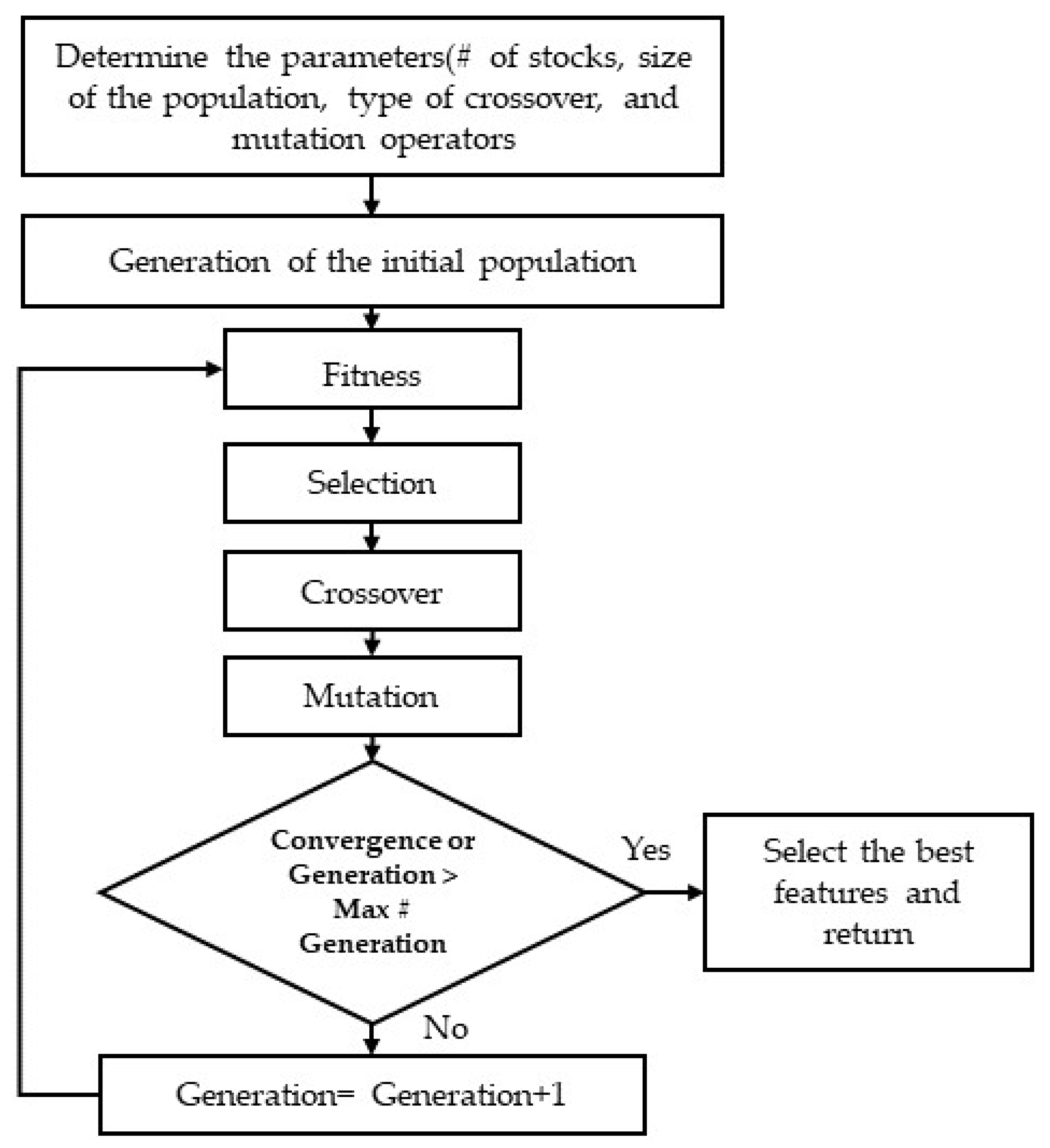
The process is to apply the filter stage for minimizing the number of features in a subset. This follows the wrapper stage that uses several local or global search algorithms. Because of the benefits listed above, the hybrid approaches are increasingly attracting the attention of many researchers. In recent years, evolutionary algorithms have achieved a great deal of attention for their capacity to solve FS such as Genetic Algorithm (GA) which is gaining popularity [29], Particle Swarm Optimization (PSO) [30], Artificial Bee Colony Algorithm (ABC) [31], Grey Wolf Optimizer (GWO) [32], Flower Pollination Algorithm(FP) [33], and Differential Evolution Algorithm (DE) [34].

In [35], GA was successfully implemented as a feature selection tool to reduce the data dimension. In [36], a novel feature selection technique based on bare-bones PSO (BBPSO) with mutual knowledge was suggested. The findings showed that the suggested method achieves a superior feature subset and is a highly competitive FS algorithm. Furthermore, a multiobjective PSO-based approach for ranking features based on their frequency (RFPSOFS) in the archive set was proposed [37]. These rankings were utilized to fine-tune the archive set. A system for feature selection based on multiobjective Gray Wolf Optimization was proposed in [38]. The proposed system depended on the data description and the classifier used, and it achieved much robustness and stability compared against different common searching methods such as particle swarm optimization and genetic algorithm. ZorarpacI and Özel proposed a hybrid approach of Differential Evolution and Artificial Bee Colony for feature selection [34], the proposed method’s performance was also compared to research in the literature that uses the same datasets. The experimental results showed that the proposed hybrid technique can select excellent features for classification tasks to increase the classifier’s run-time performance and accuracy. To predict rock tensile strength, a new artificial neural network (ANN)-based model with Invasive Weed Optimization (IWO) was proposed in [39]. The suggested hybrid of the IWO–ANN model showed a greater degree of prediction accuracy. Using FTIR and NIR datasets, Invasive Weed Optimization (IWO) was also applied to create a simple and creative variable selection approach [40]. The results showed that the performance of IWO was robust. In [39], a prediction model was proposed using Invasive Weed Optimization (IWO) with Technique-Based Artificial neural network (ANN) for rock tensile strength; the results showed that the IWO–ANN model is a suitable alternative solution for a robust and reliable engineering design. An efficient swarm intelligence approach to feature selection based on Invasive Weed Optimization (IWO) was proposed in [40]; the result has been shown to be very adaptive and powerful to environmental changes.

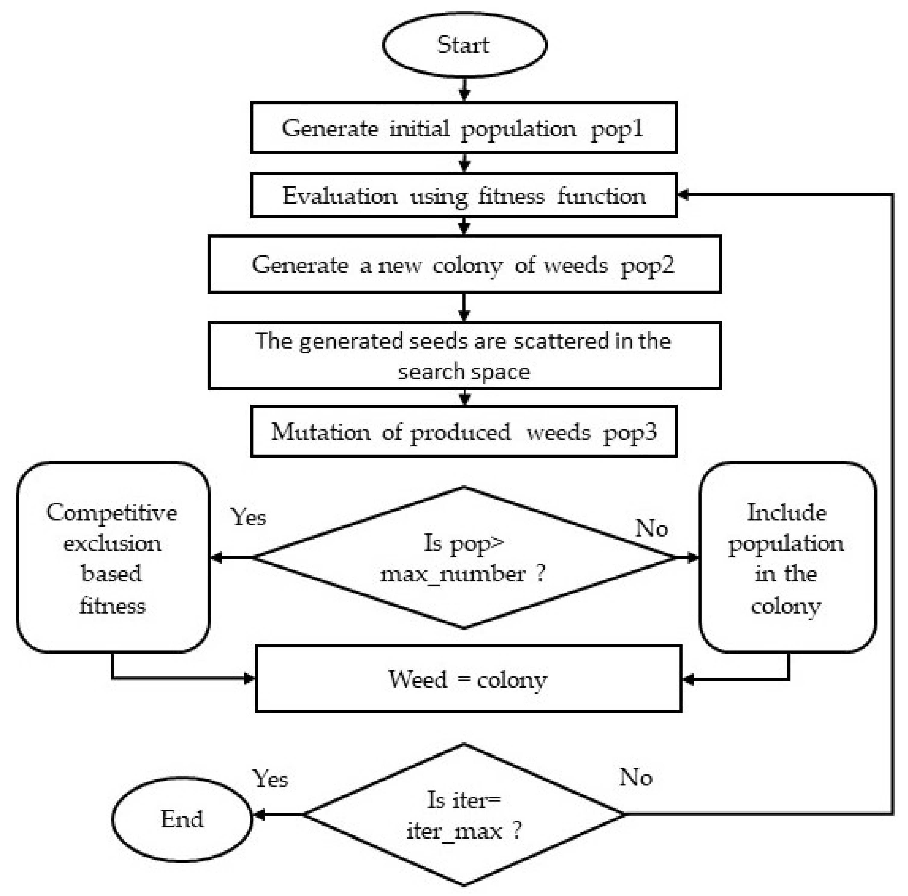
A feature selection technique based on the Invasive Weed Optimization algorithm (IWO) has been implemented in a few applications to decrease the number of obtained features and achieve both a strong learning process and low classification error. Invasive Weed Optimization (IWO) is a continuous stochastic numerical algorithm that was proposed by Locas [41]. It is a swarm intelligence metaheuristic algorithm that is inspired by the invasive weed’s colonization behaviour along the journey to find an appropriate place for growth and reproduction. This technique offers several advantages, including a simple structure, easily understood, and program characteristics. Moreover, the results achieved by using this algorithm are quite reliable.

Concisely, the main investigation of the present work is to extend the proposed work in [42]:

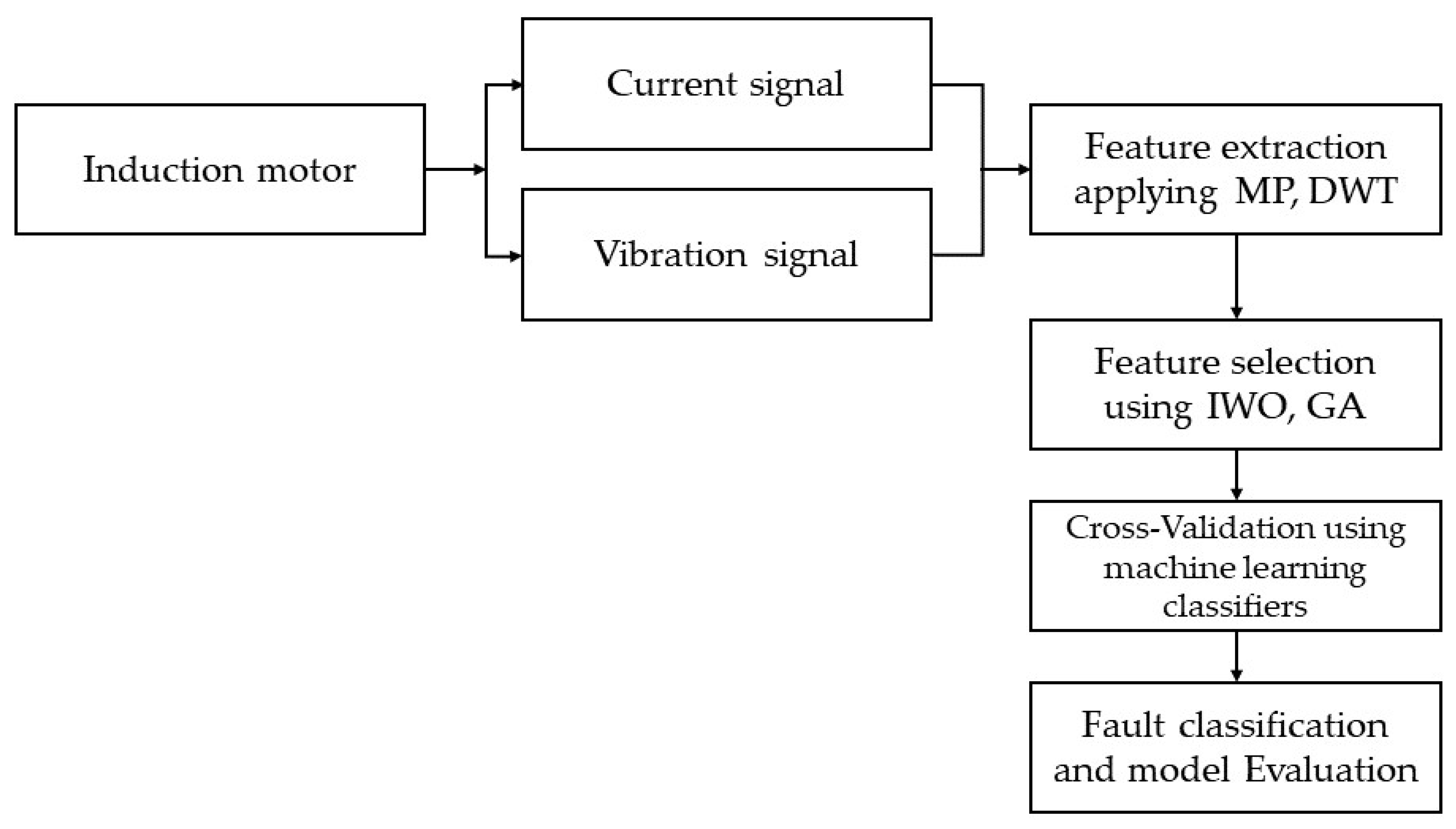
• An effective machine learning system-based fault diagnosis of induction motor using experimental data is suggested.
• Both the current and vibration motor signals are selected to be recorded simultaneously for condition monitoring.
• As the different motor loadings between the training and testing processes can deeply influence the fault diagnosis [15], experiments in this study were conducted for three motor loadings, namely 0% no-load, 50% half-load, and 100% full load to investigate the impact of the operating conditions.
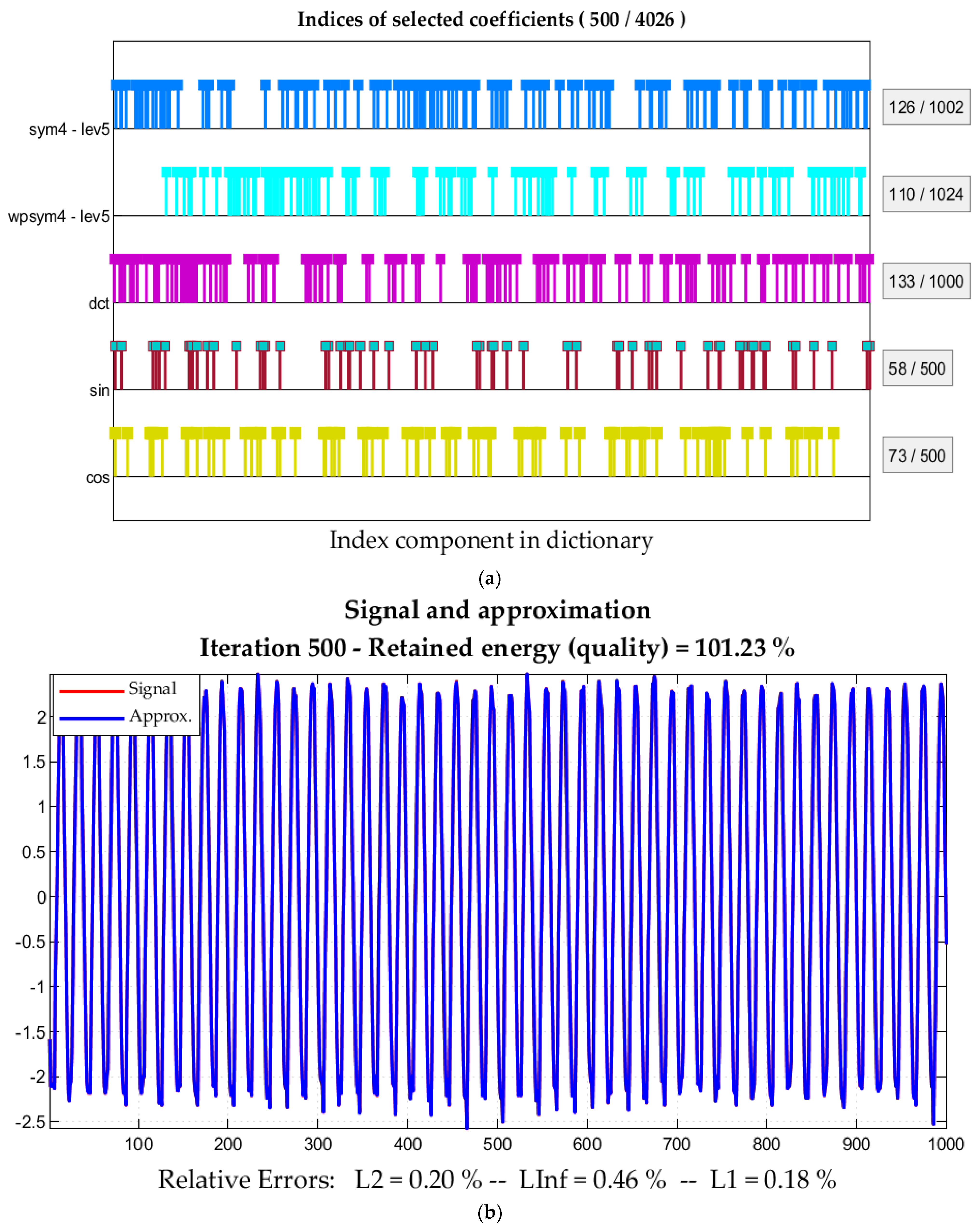
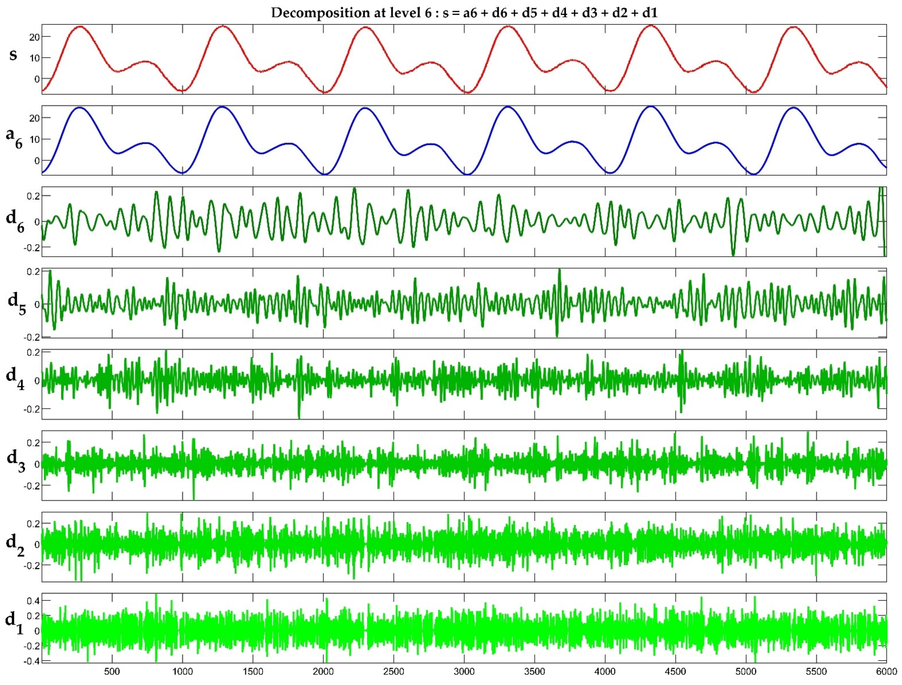
• Matching Pursuit (MP) and Discrete Wavelet Transform (DWT) in the time-frequency domain are applied for features extraction.
• Some statistical features such as mean, median, standard deviation, and others were calculated from the raw signals.
• A comparison of study-based feature selection methods using the Invasive Weed Optimization algorithm (IWO) and Genetic Algorithm (GA) was performed to reduce the number of the extracted features.
• This research investigates the classification results of three different algorithms: k-Nearest Neighbour (KNN), Support Vector Machine (SVM), and Random Forest (RF) that were trained using k-fold cross-validation.

The rest of this paper is organized as follows: Section 2 presents methods that include information about the experimental testbed and dataset collection in the lab; Section 3 presents the research methodology and the suggested model in this research; Section 4 provides the results that validate the proposed model with comparisons; Section 5 presents the discussion; and lastly, a conclusion with future work is drawn in Section 6.

2. Materials and Methods

2.1. Bearing Damage

In rolling bearings, rolling elements such as balls or cylindrical rollers are placed between the inner and outer races. Pitting or flaking can occur in the bearing components, due to wearing or material fatigue [1]. That means if there is any early damage to the bearing, shock pulses with certain frequencies appear in the frequency domain. These characteristic frequencies are dependent on the affected section of the bearing and can be determined by using the geometry and the mechanical rotational frequency ${\mathrm{f}}_{\mathrm{m}}$. The characteristic frequencies of each types of fault are calculated in the frequency domain as in the following equations [43]:

$${\mathrm{F}}_{\mathrm{Outer} \mathrm{Race} \mathrm{defect} } = \frac{{\mathrm{N}}_{\mathrm{ball} } }{2}·{\mathrm{f}}_{\mathrm{m}}(1-\frac{{\mathrm{D}}_{\mathrm{ball}}}{{\mathrm{D}}_{\mathrm{cage}}}\cos \left(\mathsf{\beta }\right))$$

(1)

$${\mathrm{F}}_{\mathrm{Inner} \mathrm{Race} \mathrm{defect} }= \frac{{\mathrm{N}}_{\mathrm{ball} } }{2}·{\mathrm{f}}_{\mathrm{m}}(1+\frac{{\mathrm{D}}_{\mathrm{ball}}}{{\mathrm{D}}_{\mathrm{cage}}}\cos \left(\mathsf{\beta }\right))$$

(2)

$${\mathrm{F}}_{\mathrm{Ball} \mathrm{defect}} =\frac{{\mathrm{D}}_{\mathrm{cage}} }{{\mathrm{D}}_{\mathrm{ball}}}·{\mathrm{f}}_{\mathrm{m}}\left(1-\frac{{\mathrm{D}}_{\mathrm{ball}}{}^2}{{\mathrm{D}}_{\mathrm{cage}}{}^2}{\cos }^2(\mathsf{\beta })\right)$$

(3)

$${\mathrm{F}}_{\mathrm{cage} \mathrm{defect} }= \frac{ 1}{2}·{\mathrm{f}}_{\mathrm{m}} (1-\frac{{\mathrm{D}}_{\mathrm{ball}}}{{\mathrm{D}}_{\mathrm{cage}}}\cos \left(\mathsf{\beta }\right))$$

(4)

where as $\mathsf{\beta }$ is the contact angle of the balls, ${\mathrm{N}}_{\mathrm{ball} }$ is the number of balls or cylindrical rollers, mechanical rotational frequency ${\mathrm{f}}_{\mathrm{m}}$, ${\mathrm{D}}_{\mathrm{ball} }$ is the diameter of the ball, and ${\mathrm{D}}_{\mathrm{cage} }$ is the ball pitch diameter.

2.2. Broken Rotor Bar Damage

Rotor bar and its bearing have undergone significant alterations. However, stator core, stator windings, and housing structure have all been left out and no significant adjustments have been made to them. Broken Rotor Bar (BRB) fault can occur due to the following aspects: thermal unbalance, over-loaded during starting, frequent start at rated voltage thermal stress [44].

If a BRB fault occurs, the current flow in that bar will be interrupted. As a result, the near faulty bar in the rotor will be inaccessible. Therefore, the response to this imbalance, an Unbalanced Magnetic Pull (UMP), is generated and rotates at the same rate as the rotating speed. It modulates at a frequency that is the same as several slip frequencies and has several poles.

Frequencies components in the frequency domain of broken rotor bars being induced in the stator winding can be visible around the principal slot harmonics in the current spectrum as follows:

$${\mathrm{f}}_{\mathrm{brb}}=\mathrm{fs} (1 \pm 2\mathrm{ks}) \mathrm{Hz}$$

(5)

where fs represents the supply frequency, k is an integer, and s indicates the slip.

These sidebands frequencies are dynamic and vary with the operating condition of the motors [45].

2.3. Stator Damage

Stator faults can be categorized as stator winding: stator core laminations, and the frame of the stator. The frequency components that can appear in the frequency domain due to this fault in the current spectrum are given by [46]:

$${\mathrm{f}}_{\mathrm{st}}=\{\mathrm{k}\mp \frac{\mathrm{n}\left(1-\mathrm{s}\right)}{\mathrm{p}}\}{\mathrm{f}}_{\mathrm{s}}$$

(6)

where ${\mathrm{f}}_{\mathrm{st}}$ short turns frequency, ${\mathrm{f}}_{\mathrm{s}}$ is the supply frequency, p is the number of pole pairs, k = 1, 3, 5; n = 1, 2.

2.4. Experimental Testbed

The dataset used in this work was obtained from Three-Phase Squirrel Cage Induction Motor (Clarke motor 80B/4, Cardiff, UK). The proposed work was executed at Wolfson Centre for Magnetics, Machines and Transformers Laboratory, Cardiff University, UK. The stator current and vibration signals were chosen in this research to be recorded because any initial motor faults can create unbalance inside the motor, which will be immediately reflected on stator currents and vibration signals.

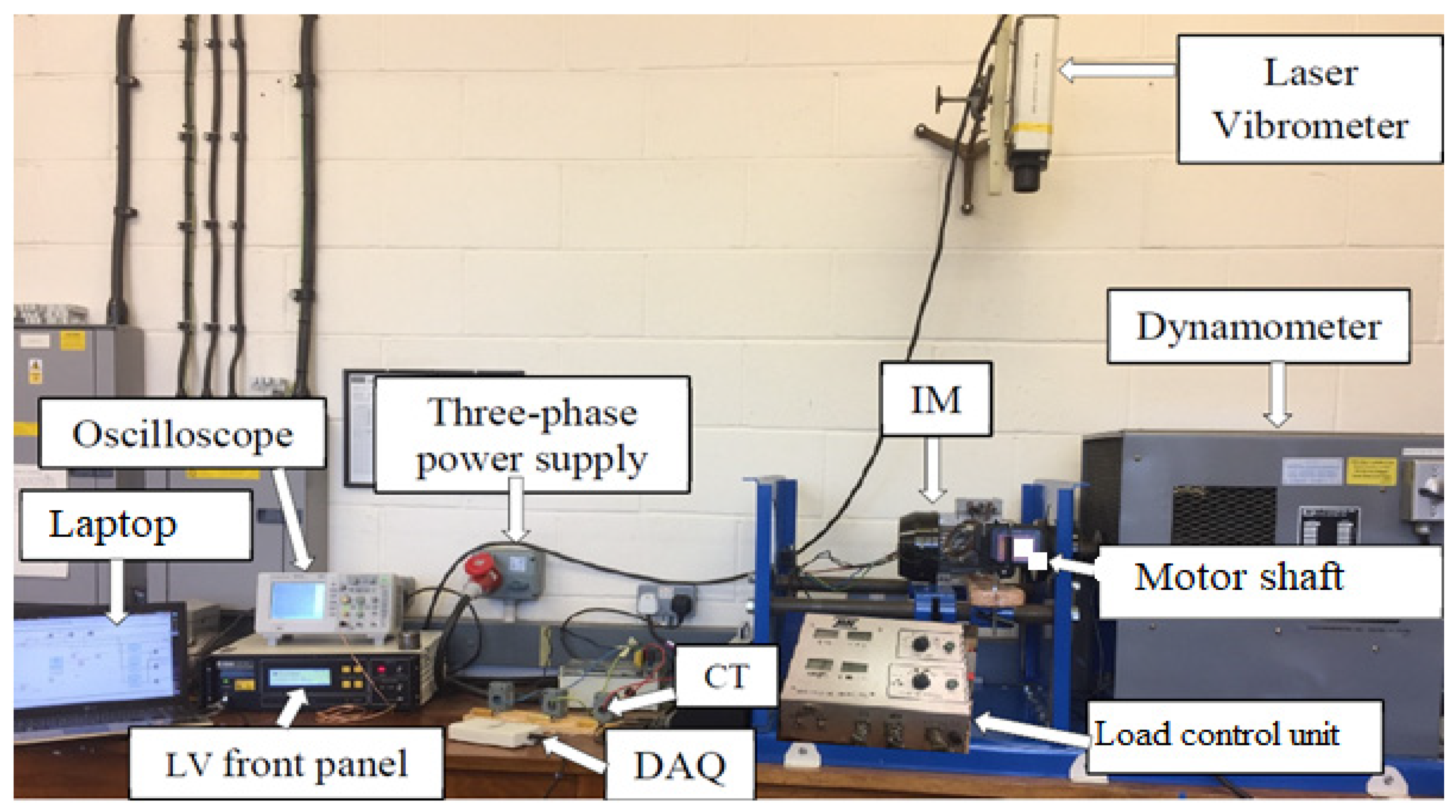
The test rig shown in Figure 1 consisted of a 4-pole, 50 Hz, 0.75-HP, 230/400 V, 1380 rev/min (Model Clarke 6430439) induction motor that was connected to a dynamometer that can allow the motor load to be controlled through the application of opposite torque and to be adjusted by the dynamometer’s control knob. The dynamometer also displays the rotational speed of the motor in revolutions per minute (RPM).

In order to collect the motor vibration signal, an overhead laser vibrometer (model OFV-3001) was utilized. The vibrometer was connected to an oscilloscope that displayed the vibration signal on a screen. Two important factors in the vibration measurement need to be calibrated before collecting the data, which are velocity and displacement range. The first one has been set to 25 mm/s/V and the latter was set to 125 μm/V.

To record the current signal passing through the motor stator, a current transformer was connected between the motor and the data acquisition card (NATIONAL IN-STRUMENTS IN USB-6211).

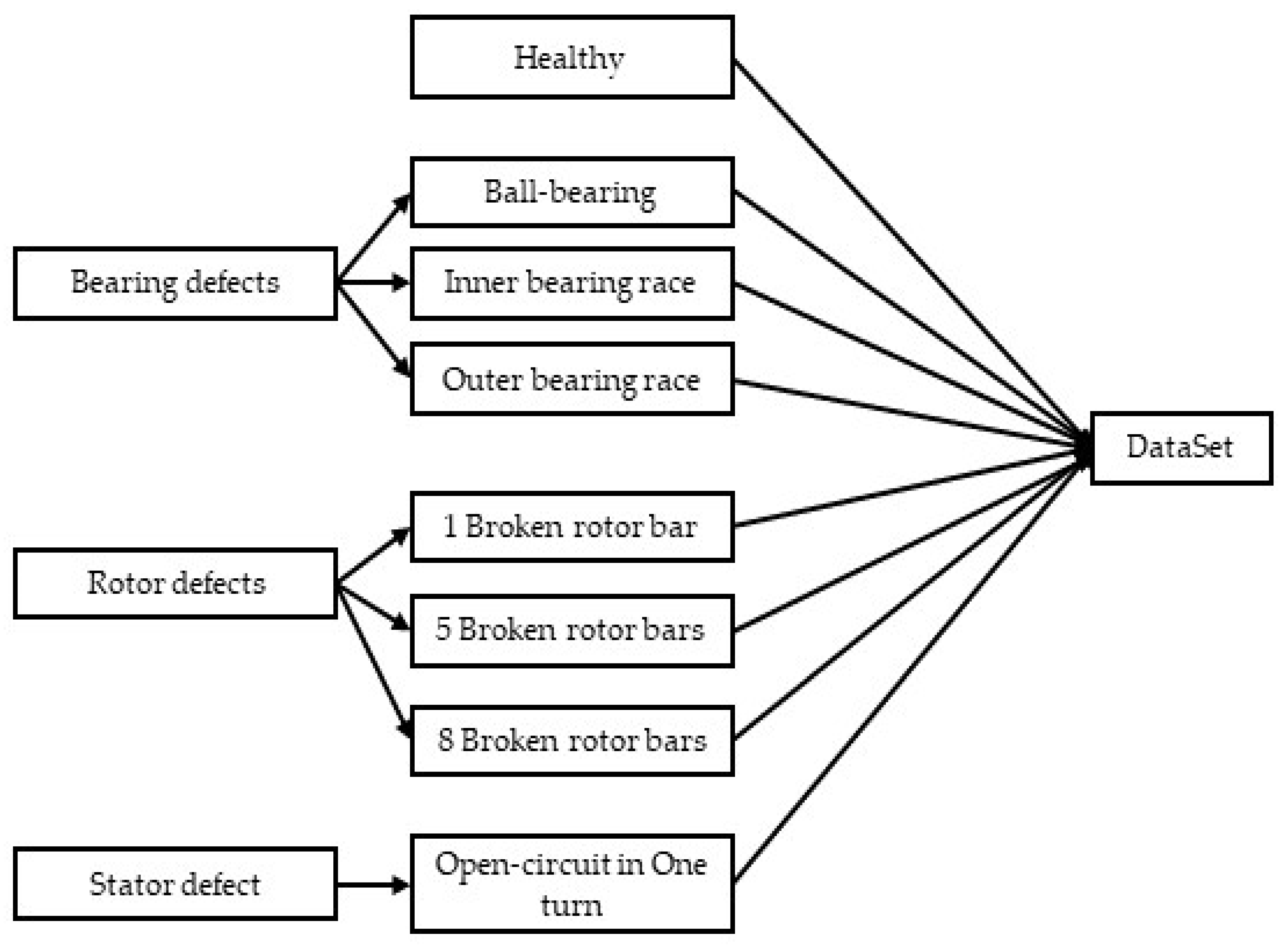
The current and the vibration signals were recorded to produce a dataset that included both the healthy and faulty behaviours of the induction motor. Three categories of motor defects are proposed in this work that are artificially generated in the lab, including bearing defect, broken rotor bar defect, and stator defects. 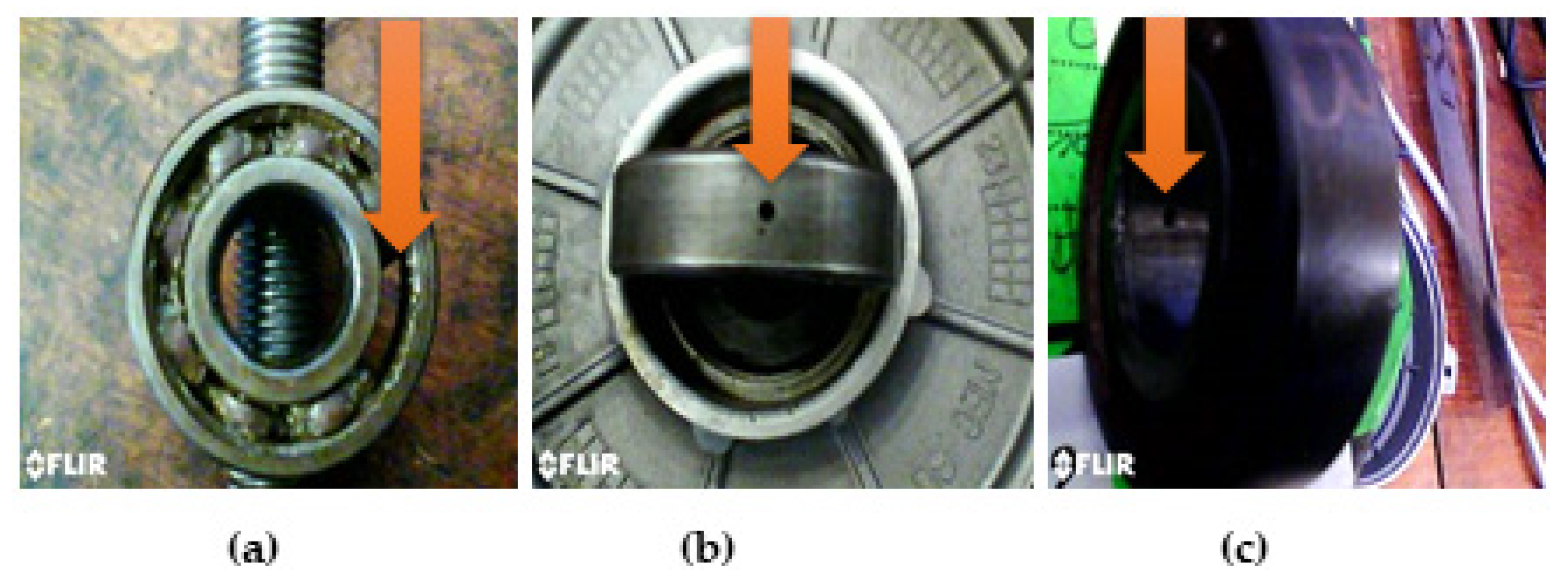Including the healthy case, data were collected for eight different motor conditions as shown in Figure 2. The ball bearing fault was created by removing one ball with its cage as shown in Figure 3a, the outer bearing fault was made by drilling a 0.25 cm hole into the outer bearing race as demonstrated in Figure 3b, and the inner bearing fault was generated by drilling the same hole into the inner bearing race as shown in Figure 3c.

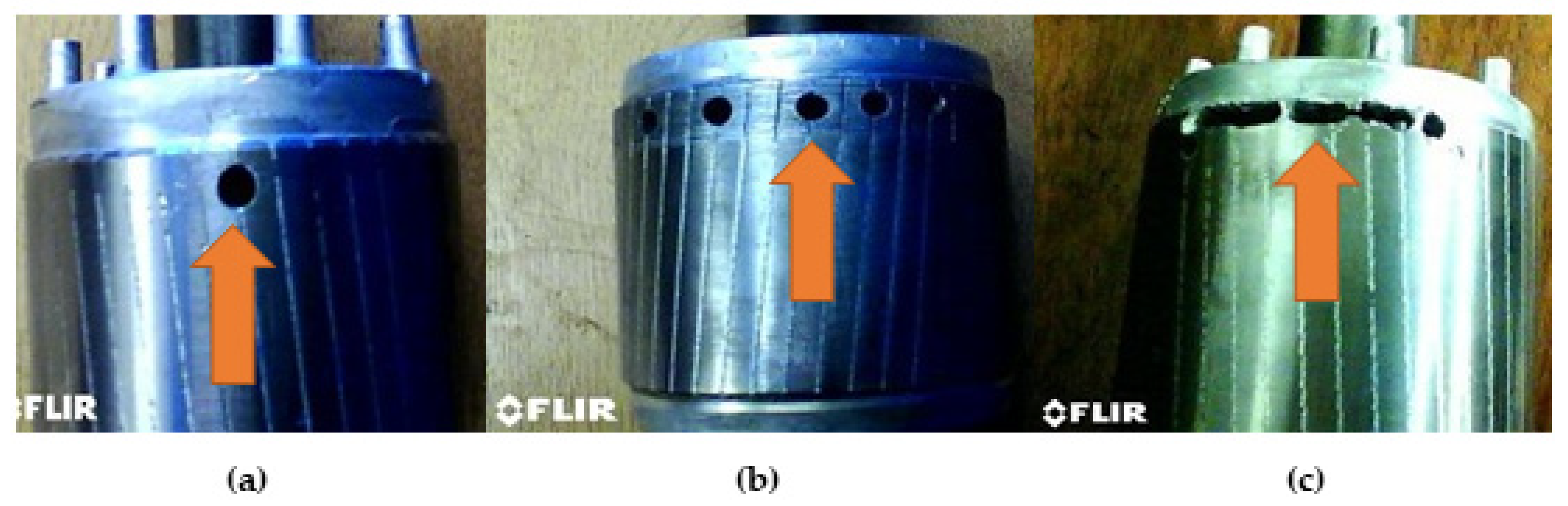
One_Broken Rotor Bar fault (1BRB) was produced artificially by drilling a hole with 4.2 mm diameter and a 16 mm depth dimension in the rotor bar to cut the bar resistance as presented in Figure 4a. The Five-Broken Rotor Bar (5BRB) and Eight-Broken Rotor Bar (8BRB) faults were created with the same diameter and depth dimensions used for One-Broken Rotor Bar (1BRB) fault, and the holes were separated by a certain angle as displayed in Figure 4b,c, respectively. The stator fault was an open circuit in one turn of the stator winding.

A test rig was set and operated under various speed conditions to investigate the impact of the operating conditions on the proposed model. The load applied to the motor may be determined by looking at the rotational speed of the motor, as the rotational speed of the motor decreases as the load increases. Three different speeds were considered during these experiments: 1480 rpm (no-load), 1450 rpm (half-load), 1380 rpm (full-load). In this study, the full-load was set as 1380 rpm, because it is the rated speed of the used induction motor, and it is unlikely that this load would be exceeded under normal industrial operating conditions. The half-load was set to speed 1450 rpm, and no-load was when the motor ran without loading at speed 1480 rpm.

2.5. Dataset Acquisition

In this section, the induction motor was placed inside the experimental test rig. A large part of the data capture process was executed with the proposed materials. The motor phase currents and the vibration signals were acquired. Several experimental measurements, each for 20 s, were taken for every motor condition as presented in

Table 1. Motor condition sets for experiments.

Case	Machine Conditions	Class Label	Load Condition
1	Healthy Motor	0	3
2	One-Broken Rotor Bar Fault	1	3
3	Five -Broken Rotor Bar Fault	2	3
4	Eight -Broken Rotor Bar Fault	3	3
5	Ball Bearing Fault	4	3
6	Inner Bearing Fault	5	3
7	Outer Bearing Fault	6	3
8	Stator Fault	7	3
Total number of motor run			27

. As all the stator current and the vibration measurement equipment have a USB connection, the obtained signals were recorded and stored in flash memory.

The sampling frequency for vibration measurements was 15 kHz and the number of sampled data of the current measurements was 20,365 points with maximum frequency of 2 kHz. In each test, three-phase stator currents (${\mathrm{I}}_1$, ${\mathrm{I}}_2$, and ${\mathrm{I}}_3$) and vibration signals were recorded simultaneously considering different load conditions by changing the rotational speeds through the use of an eddy-current brake.

3. Research Methodology

This section contains three basic steps: Feature extraction, Selection methods, and Classification Techniques.

3.1. Feature Extraction

In this paper, two efficient signal processing techniques matching pursuit (MP) and Discrete Wavelet Transform (DWT) were implemented for feature extraction through wavelet analyser toolbox in MATLAB software version R2021a with specialized tools 1-D for MP, and one-dimensional wavelet for DWT.

3.1.1. Matching Pursuit (MP)

Matching Pursuit (MP) is a multiscale decomposition technique based on an over-complete dictionary [39]. MP decomposes a signal into a linear arrangement of waveforms, known as atoms, which are taken from a redundant dictionary of functions to match the original signal as closely as possible in time frequency [43,44].

3.1.2. Discrete Wavelet Transform (DWT)

Wavelet Transform (WT) is a powerful technique that transforms raw signals in the time-frequency domain and delivers information in both time and frequency at the same time [39]. It has gained a great deal of attention in many fields, particularly as a powerful analysis instrument for machines’ fault detection and diagnosis. Wavelet was proposed in mathematics by Morlet (1984) [37]. Wavelet Transform analysis has been developed to overcome the resolution problems in some traditional methods such as STFT and discover the hidden information of the signal. WT uses a multiscale signal through translation and dilation in both time and frequency domains, rather than FFT and other transformation functions. This technique denoises a signal without causing any noticeable degradation, and it provides precise information on the location of energy content in time and frequency.

Discrete Wavelet Transform (DWT) has been widely used for analysing many signals such as electromyography, thermal image, current, and vibration signals [10]. The most important part of DWT is that it uses discrete data as a scale parameter. The discretization of the scale parameter and time parameter leads to the Discrete Wavelet Transform as defined below:

$$\mathrm{WTx}\left(\mathrm{t},\mathrm{a}\right)=\frac{1}{\sqrt{\mathrm{a}} }{{\displaystyle \int }}_{-\infty }^{+\infty }\mathrm{x}\left(\mathsf{\tau }\right)\mathsf{\psi }\left(\frac{\left(\mathrm{t}-\mathsf{\tau }\right)}{\mathrm{a}}\right)\mathrm{d}\mathsf{\tau }$$

(7)

where wavelet $\mathsf{\psi }\left(\frac{\left(\mathrm{t}-\mathsf{\tau }\right)}{\mathrm{a}}\right)$ is derived by dilating and translating the wavelet basis ψ(t), a is the scale parameter, t is the time shift, and $\frac{1}{\sqrt{\mathrm{a}} }$ is a normalization factor.

$$\mathrm{W}\left(\mathrm{m},\mathrm{n},\mathsf{\Psi }\right)={\mathrm{a}}_0^{\frac{-\mathrm{m}}{2}}{\displaystyle \int }\mathrm{x}\left(\mathrm{t}\right)\mathsf{\Psi }\ast \left({\mathrm{a}}_0^{-\mathrm{m}}\mathrm{t}-{\mathrm{nb}}_0\right) \mathrm{dt}$$

(8)

where x(t) is the raw signal, m and n are integers, the scale a and the time b are described as below:

$$\mathrm{a}={\mathrm{a}}_0^{\mathrm{m}}, \mathrm{b}=\mathrm{n}{\mathrm{a}}_0^{\mathrm{m}}{\mathrm{b}}_0$$

(9)

DWT decomposes the signal into multiresolution coefficients, where the features are extracted from each coefficient to develop the feature vector. The signal is decomposed into multiresolution coefficients using a low pass filter as well as a high pass filter.

The coefficients of the decomposed single are included in different frequencies. In case the coefficients are with higher frequency, it is detail coefficients (D). Conversely, when the coefficients are at a lower frequency it is labelled as approximation coefficients (A), which achieves a better resolution frequency field. This can be formulated as given in the equations below:

$$\mathrm{Z}\_\mathrm{high}={\displaystyle \sum }\mathrm{x}\left[\mathrm{k}\right]·\mathrm{g}\left[2\mathrm{k}-\mathrm{n}\right]$$

(10)

$$\mathrm{Z}\_\mathrm{low}={\displaystyle \sum }\mathrm{x}\left[\mathrm{k}\right]·\mathrm{h}\left[2\mathrm{k}-\mathrm{n}\right]$$

(11)

where Z_low denotes the approximation coefficients and Z_high is the detail, x[k] represents the input of collected signal, and $\mathrm{g}\left[2\mathrm{k}-\mathrm{n}\right]$ and $\mathrm{h}\left[2\mathrm{k}-\mathrm{n}\right]$ are the low pass filter and the high pass filter; respectively. The decompensation level is selected based on the maximum level where at least one coefficient in the output is uncorrupted by edge effects caused by a signal extension. It can be calculated as given in the formula below:

$$\mathrm{Max}\_\mathrm{level}=[{ \log }_2\frac{\mathrm{data}\_\mathrm{len}}{\mathrm{filter}\_\mathrm{len} -1} ]$$

(12)

where the filter_len is an integer and can be the name of the wavelet object.

3.1.3. Decomposition Using (MP)

In this work, the Orthogonal Matching Pursuit (OMP) algorithm was executed using five signal components of the OMP dictionary as tabulated in

Table 2. Orthogonal Matching Pursuit (OMP) components [39].

Dectionary Parameter	Definition
sym4-lev5	Symmetric wavelet transform with five levels and four vanished moments
wpsym4-lev5	wavelet packet based symmetric at four vanished moments with five levels
Dct	Discrete cosine transform
Sin	Sine sub dictionary
Cos	Cosine sub dectionary

. The collected stator current at the second phase (${\mathrm{I}}_2$) with the vibration signal was simply applied under healthy and faulty cases to be processed using OMP provided by the MATLAB toolbox. In MATLAB toolbox, some OMP parameters have been carefully set, such as max iteration = 100, max relative error = L1 norm with 0.01%.

Eight statistical features were determined using OMP as follows: mean, median, standard deviation, median absolute deviation, mean absolute deviation, L1 norm, L2 norm, and the maximum norm as illustrated in the below equations.

$$\mathrm{Mean} \mathsf{\mu }=\frac{1}{\mathrm{N}}{{\displaystyle \sum }}_1^{\mathrm{N}}{\mathrm{x}}_{\mathrm{i}}$$

(13)

$$\mathrm{Median} \mathrm{med}=\frac{1}{2}(\mathrm{x}([\frac{(\mathrm{N}+1)}{2}])+\mathrm{x}([\frac{\mathrm{N}}{2}]1))$$

(14)

$$\mathrm{Standard} \mathrm{deviation} \mathsf{\sigma }=\sqrt{\frac{{{\displaystyle \sum }}_{\mathrm{i}=1}^{\mathrm{N}}{\left({\mathrm{x}}_{\mathrm{i}}-\mathsf{\mu }\right)}^2}{\mathrm{N}-1}}$$

(15)

Median Absolute Deviation med_AD = median(|xi-median(X)|)

(16)

$$\mathrm{Mean} \mathrm{Absolute} \mathrm{Deviation} {\mathsf{\sigma }}^2=\frac{{{\displaystyle \sum }}_{\mathrm{i}=1}^{\mathrm{N}}{\left({\mathrm{x}}_{\mathrm{i}}-\mathsf{\mu }\right)}^2}{\mathrm{N}-1}$$

(17)

$$\mathrm{L}1 \mathrm{norm} \Vert \mathrm{L}\Vert 1={{\displaystyle \sum }}_{\mathrm{i}-1}^{\mathrm{N}}{\mathrm{x}}_{\mathrm{i}}$$

(18)

$$\mathrm{L}2 \mathrm{norm} \Vert \mathrm{L}\Vert 2=\sqrt{{{\displaystyle \sum }}_{\mathrm{i}=1}^{\mathrm{N}}{|{\mathrm{x}}_{\mathrm{i}}|}^2}$$

(19)

$$\mathrm{Max} \mathrm{norm} \Vert \mathrm{L}\Vert \infty =\max \left\{\right|{\mathrm{x}}_{\mathrm{i}}\left|\right\}$$

(20)

where ${\mathrm{x}}_{\mathrm{i}}$ is the sampled acquired signal, i = 1, 2, 3, …, N, L1 norm is the sum of absolute values of its components, L2 norm is the square root of the sum of absolute values of its components, and the maximum of the absolute values of its components is also known as infinity norm.

In order to validate OMP processing results, an example with One-Broken Rotor Bar fault at speed 1480 RPM applying 1000 sample points of the current signal is displayed in Figure 5.

3.1.4. Decomposition Using (DWT)

Among the various types of the wavelet transform, Discrete Wavelet Transform (DWT) has proved its power to extract the initial features in many applications of induction-motor fault diagnosis [45,46]. The procedure of wavelet decomposition at n level decomposition is to analyse the approximation signal in each level which is continued until the desired level n is reached.

In this work, five mother wavelets were adopted to analyse both the stator current and the vibration signals, namely [15], db7, sym3, coif4, bior6.8, and rbior6.8 that were provided by MATLAB Toolbox. The decomposition of six levels was carried out. The acquired motor signals were simply applied to the DWT approach for obtaining the initial energy features. Thirty features applying all the proposed five-mother wavelets were extracted in the time-frequency domain separately. These data are stored in a matrix with 2000 rows (sampled signals) and 30 columns (attributes), which will be used later to build the proposed datasets.

In order to validate the DWT processing results, one-Broken Rotor Bar fault conditions of the motor vibration signals operating at speed of 1480 rpm are illustrated in Figure 6. A combination of fourteen statistical features including the original signals of the stator current and motor vibration were extracted using OMP and DWT to build a feature matrix of 1800 × 40 as given in

Table 3. Description of datasets.

Dataset	Signal Type	No. of Total Samples	No. of Classes	Load Condition (rpm)	No. of Features
1	Current	1800	8	1480	40
2	Current	1800	8	1450	40
3	Current	1800	8	1380	40
4	Vibration	1800	8	1480	40
5	Vibration	1800	8	1450	40
6	Vibration	1800	8	1380	40
7	Current	1800	8	1480, 1450, 1380	40
8	Vibration	1800	8	1480, 1450, 1380	40

.

3.2. Feature Selection Algorithms

Feature selection is known as the process of detecting and eliminating irrelevant, less valuable, and redundant attributes, as well as discovering the most acceptable inputs for a classification model.

3.2.1. Invasive Weed Optimization (IWO)

Invasive Weed Optimization (IWO) is a swarm intelligence metaheuristic algorithm that is inspired by invasive weeds’ colonization behaviour along their journey to find an appropriate place for growth and reproduction. This technique offers several advantages, including a simple structure, easily understood, and program characteristics; moreover, the results achieved using this algorithm are quite reliable [47].

The following steps illustrate the overall process of IWO-based feature selection:

• Step 1: Generate a population of initial solution (weeds), which is referred to as pop1.
• Step 2: Each weed in the population will be evaluated using a certain fitness function.
• Step 3: Every weed reproduces new seeds. The weeds will generate seeds ${\mathrm{Seed}}_{\mathrm{i}}$ that are calculated as given in this formula:

  $${\mathrm{Seed}}_{\mathrm{i}}={\mathrm{S}}_{\min }+\left({\mathrm{S}}_{\max }+{\mathrm{S}}_{\min }\right)\times \frac{{\mathrm{fit}}_{\mathrm{worst}}-{\mathrm{fit}}_{\mathrm{i}}}{{\mathrm{fit}}_{\mathrm{worst}}-{\mathrm{fit}}_{\mathrm{best}}}$$

  (21)

  where ${\mathrm{S}}_{\min },$ and ${\mathrm{S}}_{\max }$ are the minimum and maximum possible numbers of produced seeds for the worst and best weeds. ${\mathrm{fit}}_{\mathrm{worst}}$ and ${\mathrm{fit}}_{\mathrm{best}}$ are the fitness values for the worst and best weeds in the colony; Fir_i refers to the fitness value of the weeds in the colony.
• Step 4: Spatial dispersal where randomness and adaptation are incorporated into the algorithm. The generated seeds are scattered in the search space, and spatial dispersion performance can be given by the following equation:

  $$\mathrm{SDiter}=\frac{{\left({\mathrm{iter}}_{\max }-\mathrm{iter}\right)}^{\mathrm{n}}\times \left({\mathrm{SD}}_{\mathrm{initial}}-{ \mathrm{SD}}_{\mathrm{final}}\right)}{{\left({\mathrm{iter}}_{\max }\right)}^{\mathrm{n}}}+{ \mathrm{SD}}_{\mathrm{final}}$$

  (22)

  where ${\mathrm{iter}}_{\max }$ is the maximum number of iterations, and n is the index of nonlinear modulation.
• Step 5: Performing the local search method where the mutation can be applied to prevent premature convergence. The population resulting from mutation operation is named pop3 and its size is equal to that of pop2.
• Step 6: An affinity function was applied to avoid premature convergence and extend the diversification.
• Step 7: The competitive step is implemented to eliminate the weeds with poor fitness values when the maximum population size is reached in the colony. This process will be continueed till the iteratiotion value is reached. These steps can be summarised in the block diagram given (see Appendix A).

In this study, the feature selection algorithm IWO was adopted to select the best features. The procedure was run for 100 generations to find the best values parameters of IWO. The IWO parameters that were finalized are listed in

Table 4. The invasive weed optimization parameter settings for feature selection [45].

Parameter Name	Values
Initial populations No.	5
Maximum weed population No.	25
Minimum number of seeds	1
Maximum number of seeds	15
Nonlinear modulation index	3
Initial value of standard deviation	1
The final value of standard deviation	0.001
Fitness Function	Classification KNN error
Maximum Generation No.	100

.

3.2.2. Genetic Algorithm (GA)

Holland in 1995 proposed the GA based feature selection [46]. A heuristic search is employed by the GA-based features selection method to establish a good balance between computational cost and optimum selection. It can be simply parallelized in computer clusters and a large amount of data not including any prior understanding of the project. The entire procedure for GA-based feature features selection is illustrated (see Appendix B).

3.3. Classification Techniques

In this section, a couple of classification algorithms are demonstrated that are thoroughly discussed in the following subsections.

3.3.1. K-Nearest Neighbour (KNN)

KNN is the simplest machine learning classifier. It categorizes the unknown cases using correlation technique based on unknown cases and similarity function [48]. The proposed dataset that applied to this classifier is arranged in clusters based on a fixed number (k) that might be real or imaginary to train it. The centroid of the cluster is the centre data point in the classifier iterative process. The emanated classifier is used to create an initial set of random clusters and will continue to shift the centroid value until it becomes stable. Then, this model is employed to classify the new data [49].

3.3.2. Support Vector Machine (SVM)

SVM is another classifier that is widely applied for classification and regression. This algorithm divides a dataset into two categories: negative and positive groups. The statistical learning also is in use for training the proposed dataset, which is represented as a support vector [50]. This algorithm offers categorization information and constructs the hyperplane. The hyperplane optimizes the spacing between the positive and negative groups. When a dataset comprises both separable and nonseparable data profiles, SVM is an appropriate algorithm, and kernel functions for nonlinear transformation. By mapping it in a large number of features, the nonlinearly separable object is converted into a linearly separable object via the kernel function [51]. A variety of kernel functions have been utilised, including linear kernels, polynomial kernels, and Gaussian radial basis function (RBF) kernels.

3.3.3. Random Forest (RF)

The employment of ensemble approaches is motivated by the fact that the ensemble classifier is more likely to have a lower error rate or a smaller variance [52]. Random decision forests are a type of collective learning that may be used for regression and classification [53]. This approach generates a large number of decision trees during the training phase, then defines the class that is the mode of the classification classes and forecasts the mean value for regression of each tree during the testing phase. In general, the number of features control the diversity of the forest tree, so fewer features result in uncorrelated trees, and more features result in correlated trees. As a result, while a high number of trees might improve performance, they also increase the device’s size and computational cost [37].

3.4. Proposed Method

To conduct this project, a block diagram describing the main steps of the proposed application in Figure 7. The current signal and vibration signal using specialized sensors under different operating conditions are recorded to build a large dataset. Next, a combination of features is extracted adopting OMP and DWT for each collected signal to build the initial features.

As too many features can lead to too much noise, while too few features can lead to critical information being missed, selecting the number of optimal discriminative features is a vital task [21]. When a large number of features are utilised, the computational complexity of classification algorithms is excessive unless specific data dimensionality reduction methods are applied prior to the classification step [54]. As a result, this work suggests an IWO-based feature selection using the acquired feature matrix for discriminant feature selection in order to minimize data dimension. Then, further GA is applied for the same purpose to compare the results with the performance of IWO. The fitness function of these algorithms is constructed using the classification error of the KNN algorithm (K = 3).

After all, the feature matrix that obtained from the feature selection process is fed into three machine learning classifiers to conduct fault classification. next, the classifiers are trained using the Cross-Validation technique. The training was performed numerous times with 5-fold Cross-Validation and 10-fold Cross-Validation technique to fine-tune the model and verify the consistency in the results.

3.5. Model Evaluation

Different performance metrics are measured to evaluate the robustness of the model. In this research, the specificity, overall accuracy, sensitivity, prediction, F1-score, and receiver operation characteristic (ROC) curve are considered to evaluate the proposed model. These evaluation parameters are calculated as given in

Table 5. Evaluation parameters.

Case No.	Parameter	Formation
1	Specificity	$\frac{\mathrm{TN}}{\mathrm{FP}+\mathrm{TN}}$ (23)
2	Overall Accuracy	$\frac{\mathrm{TP}+\mathrm{TN}}{\mathrm{TP}+\mathrm{FP}+\mathrm{TN}+\mathrm{FN}}$ (24)
3	Precision	$\frac{\mathrm{TP}}{\mathrm{TP}+\mathrm{FP}}$ (25)
4	Sensitivity	$\frac{\mathrm{TP}}{\mathrm{TP}+\mathrm{FN}}$ (26)
5	F1_score	$2\times \frac{\mathrm{Precision} \times \mathrm{Sensitivity}}{\mathrm{Precision} + \mathrm{Sensitivity}}$ (27)

. Notethat the number of true positive forecasts is denoted by TP, the number of false positive predictions is represented by FP, the number of true negative predictions is indicated by TN, and the number of false negative predictions is expressed by FN.

Whereas the specificity denotes how accurately the assignment to the positive class is made, accuracy denotes the model’s performance; precision as well as the sensitivity indicate how appropriately the error type of the model is a positive class, and the F1-score is the harmonic mean of sensitivity and precision.

4. Results

In this section, the proposed application is assessed based on the experimental data of the current and the vibration signals.

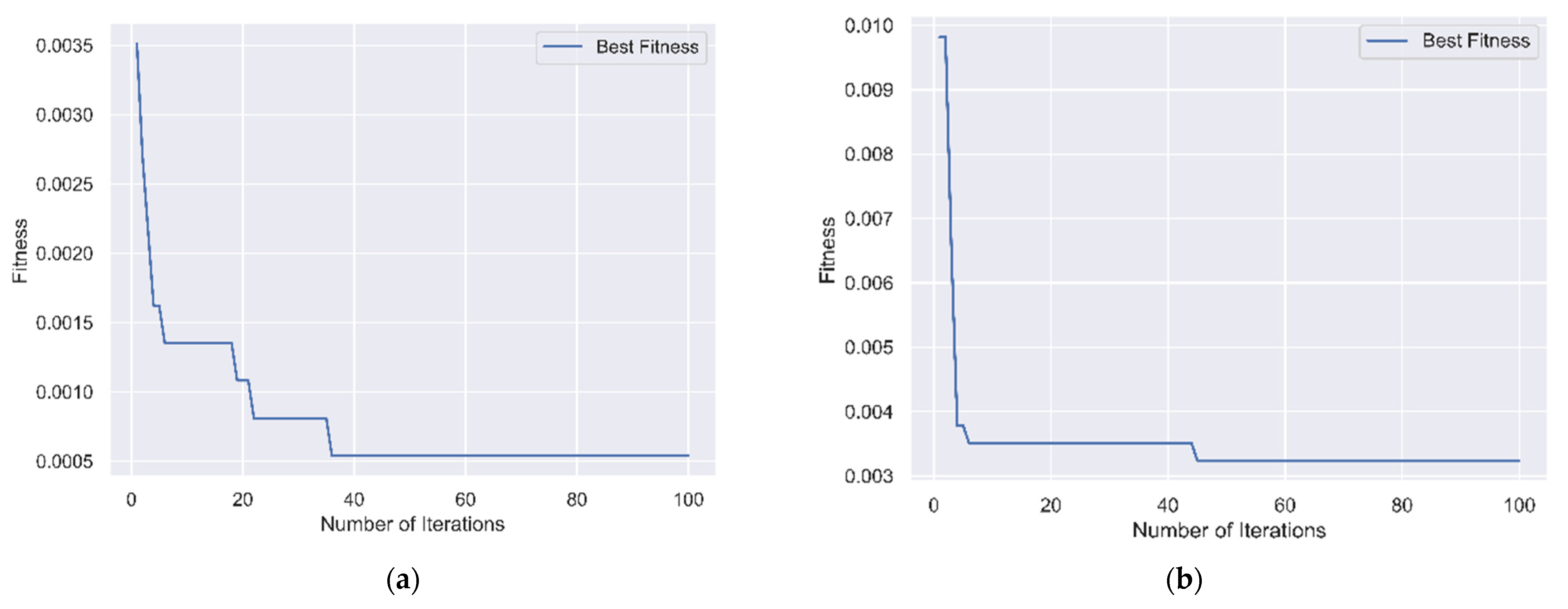
In order to verify whether the proposed model in combination with the proposed feature selection techniques to select discriminative features benefits the fault detection procedure, the acquired signals with same extracted features were used as inputs to the classification algorithms. When the current signal was applied, instead of fourteen features, invasive weed optimization (IWO) selected eight features that indexed in [5,10,11,16,22,23,29,34] with the best cost of 0.0006 as illustrated in Figure 8a for creating the final feature matrix. On the other hand, the feature index [2,4,5,7,11,14,15,17,23,26,28] selected from the vibration signal with the best fitness equal to 0.0034 is shown in Figure 8b.

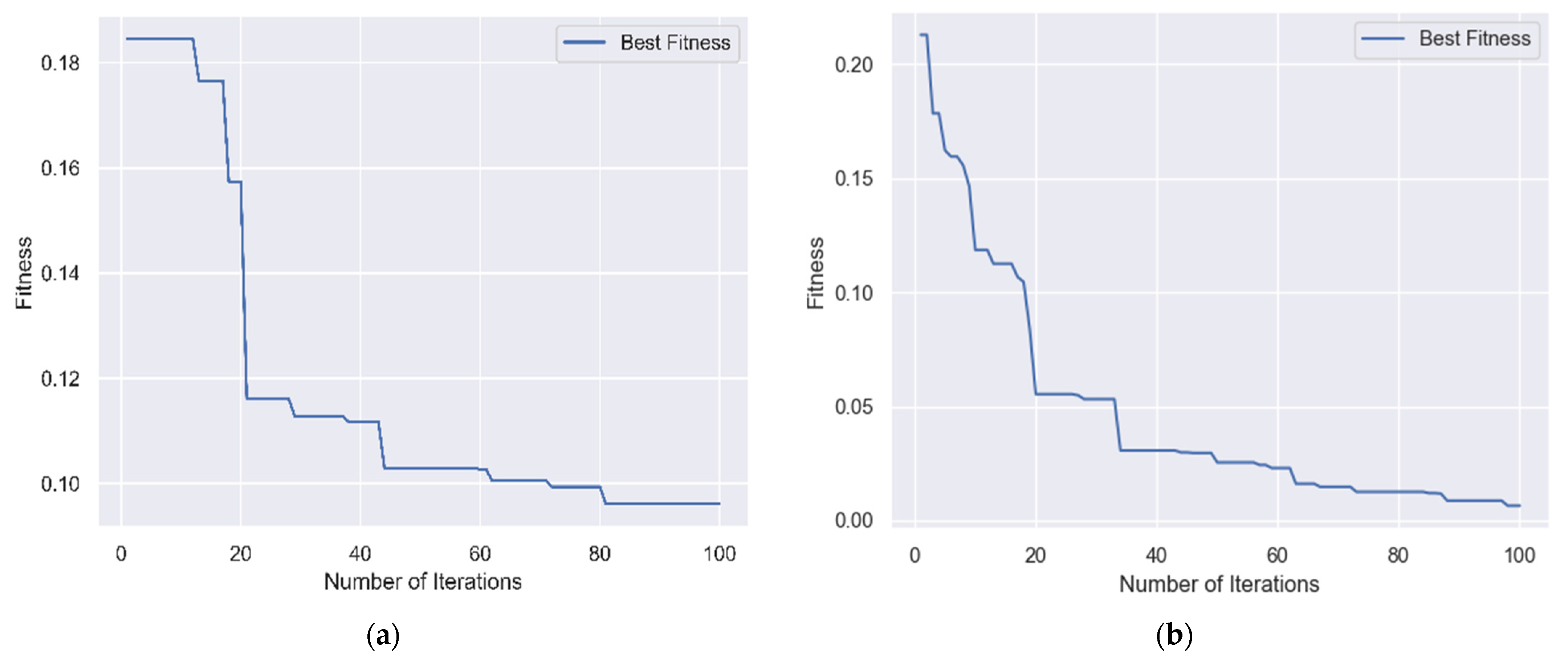
A similar pattern was conducted using Genetic Algorithm (GA) for comparing the performance and the superiority of the proposed IWO algorithm. Based on the implementation of GA using the current signal, nineteen features were carefully chosen by instead of all original features. The indexed positions of the selected features are given in the following vectors [3,5,9,10,11,12,13,14,16,17,19,21,22,23,25,26,29,33,34] with loss curve displayed in Figure 9a. A feature size of eighteen was selected from the vibration signal that indexed in [2,3,4,5,7,9,11,13,14,15,16,17,19,20,23,26,27,28] with loss curve shown in Figure 9b. As stated in

Table 6. Number of selected features.

		Number of Selected Features
Case	Algorithms	Current Signal	Vibration Signal
1	IWO	8	11
2	GA	19	18

, IWO selected a minimum of eight optimal features when the current signal was applied, and it can select eleven optimum features from the vibration signal. Moreover, GA selected a minimum series of 19 features and 18 features applying the current and the vibration signals, respectively. The classification results based on the utilization of IWO and GA for features selection are shown in

Table 7. Classification results applying Invasive Weed Optimization.

5-Fold Cross-Validation	KNN		SVM		RF
	Current	Vibration	Current	Vibration	Current	Vibration
Specificity (%)	98.1	95	99.8	98.7	99.8	99.1
Accuracy (%)	97.1	91.6	99.7	98.6	99.5	99.2
Precision (%)	93	80	99.2	97.8	98.7	98.5
Sensitivity (%)	92.3	76.3	99.2	97.8	98.7	98.5
F1-score (%)	92.2	75	99.2	97.8	98.7	98.5
10-Fold Cross-Validation	KNN		SVM		RF
	Current	Vibration	Current	Vibration	Current	Vibration
Specificity (%)	98.2	94.9	99.8	98.8	99.9	99.9
Accuracy (%)	97.1	91.5	99.7	98.6	99.9	99.7
Precision (%)	94.5	79.6	99.3	98	98.8	99
Sensitivity (%)	94.4	74.6	99.3	98	98.8	99
F1-score (%)	94.4	75	99.3	97.9	98.8	99

and

Table 8. Classification results applying genetic algorithm.

5-Fold Cross-Validation	KNN		SVM		RF
	Current	Vibration	Current	Vibration	Current	Vibration
Specificity (%)	94.1	93.5	98.6	99.3	99.8	99.7
Accuracy (%)	90.3	89.3	97.7	98.8	99.2	98.9
Precision (%)	75.7	71	93.1	96.6	99.1	98.8
Sensitivity (%)	71	67.9	93.1	96.5	99.1	98.8
F1-score (%)	71	67	93	96.5	99	98.7
10-Fold Cross-Validation	KNN		SVM		RF
	Current	Vibration	Current	Vibration	Current	Vibration
Specificity (%)	96.2	95	99	99.8	99.9	99.8
Accuracy (%)	93.7	91.8	98.4	99.4	99.6	99.1
Precision (%)	81.3	80.6	95.4	99.3	99.7	98.9
Sensitivity (%)	81.1	75.4	95.4	99.3	99.7	98.9
F1-score (%)	80.8	76.5	95.4	99.3	99.4	98.9

, respectively.

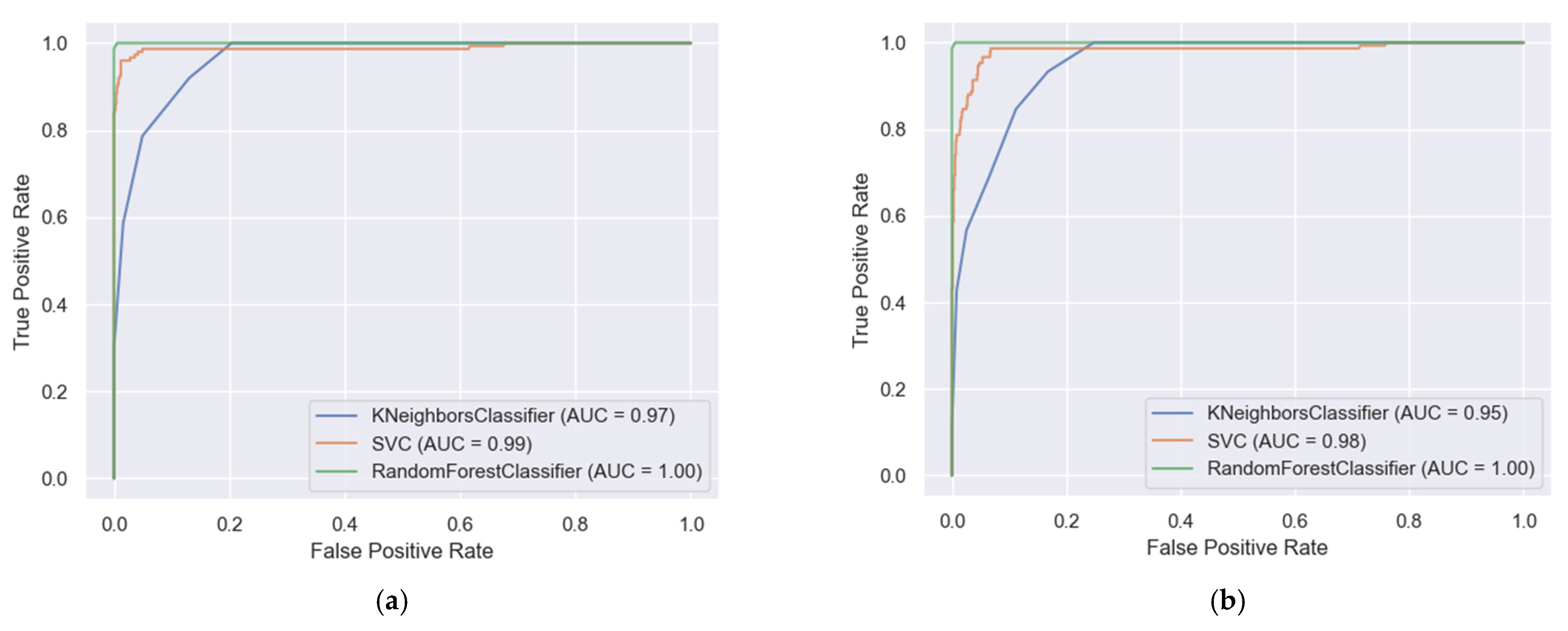
Next, the optimal feature subsets that were selected by IWO and GA were applied to three machine learning models, KNN, SVM, and RF, for classification into their respective classes. The optimum values for the parameters of KNN, SVM, and RF were properly set as follows: neighbour = 1, C = 20, kernel = RBF, and n_estimators = 250. Each classifier’s performance was evaluated using the specificity, accuracy, sensitivity, prediction, the F1-score, and receiver operating characteristic (ROC) curve. Moreover, the area under the curve (AUC) was considered in ROC because it gives an excellent indication of how well a classification model performed on a dataset. The AUC curves ranged between 0 and 1. If this value is around or less 0.5, that means the classifier has not performed well with misclassification. On the other side, when the value is close to 1, that represents the efficient model. The ROC curves of the proposed model were presented in Figure 10a,b applying the current and vibration signals, respectively.

It can be stated that the highest classification accuracy was gained by Random Forest classier (RF) which was 99.9% when the model was trained with 10-fold cross-validation by applying the current signal. And it was 99.7% when the model was trained with the same 10-fold cross-validation by applying the vibration signal. Furthermore, when the SVC model was trained with 5-fold cross-validation, the accuracy was 97.7%, and it was further raised to 98.4% when the model was trained with 10-fold cross-validation using the current signal. In addition, the classification accuracy using the KNN classifier, was less equal to 97.1% and 91.5% with 10-fold cross-validation applying the current and vibration signals, respectively. The other evaluation parameters such as specificity, precision, recall, and F1-score were given the outcome in the same representations as to the accuracy. Furthermore, The AUC score for RF was the same, which was 1 for the current and vibration signal, while it was 0.99 and 0.98 for SVC, and it was 0.97 and 0.95 for KNN, which indicates that RF and SVC models perform well in comparison with the KNN classifier.

In addition, it can be confirmed that as stated in

Table 9. Comparison between Invasive Weed Optimization and Genetic Algorithms.

10-Fold Cross-Validation		KNN		SVM		RF
	Methods	Current	Vibration	Current	Vibration	Current	Vibration
Specificity (%)	GA	96.2	95	99	99.8	99.9	99.8
	IWO	98.2	94.9	99.8	98.8	99.9	99.9
Accuracy (%)	GA	93.7	91.8	98.4	99.4	99.6	99.1
	IWO	97.1	91.5	99.7	98.6	99.9	99.7
Precision (%)	GA	81.3	80.6	95.4	99.3	99.7	98.9
	IWO	94.5	79.6	99.3	98	98.8	99
Sensitivity (%)	GA	81.1	75.4	95.4	99.3	99.7	98.9
	IWO	94.4	74.6	99.3	98	98.8	99
F1-score (%)	GA	80.8	76.5	95.4	99.3	99.4	98.9
	IWO	94.4	75	99.3	97.9	98.8	99

, RF achieved the highest accuracy by applying the current signal, which was 99.2% and 99.6% with the utilization of 5-fold and 10-fold cross-validation, respectively. Furthermore, it was 98.9 and 99.1% with the utilization of 5-fold and 10-fold cross-validation applying the vibration signal, respectively. When the model was trained using SVC, the highest accuracy was achieved with the use of 10-fold cross-validation, which was 98.4% for the current signal, and 99.4% for the vibration signal. Additionally, when the model was trained using KNN, the best accuracy was obtained using the current signal when the model was trained using 10-fold cross-validation, which was 93.7%. The other evaluation parameters represent the same outcome.

Moreover, it can be seen from Table 7 and Table 8 that both IWO and GA produced better results using 10-fold cross-validation when compared to 5-fold cross-validation. For further comparison, GA and IWO are compared against each other as shown in Table 9 applying the stator current and vibration signals. When IWO was coupled with KNN and SVM classifiers, IWO achieved better results in current signal data for all measurements.

Regarding the IWO with RF classifier (IWO–RF), IWO managed to achieve better results in vibration signal data in all evaluation measurements. However, for current data, IWO–RF can achieve similar sensitivity results and better classification accuracy against IWO–RF. Therefore, GA–RF managed to achieve better results than IWO–-RF in precision, sensitivity, and F1-score measurements.

5. Discussion

From this result, it can be concluded that the proposed model built using either current or vibration signal proves robust fault classification performance that can confirm the superiority of the proposed model. Invasive Weed Optimization (IWO) and Genetic Algorithm (GA) have reduced the data dimension with less computational complexity with the most significant features for the classification model. However, the obtained features that were selected by IWO were less than the features selected by GA, which achieves greater overall classification accuracy. In addition, in most cases the RF classifier outperforms the KNN and SVM classifiers in identifying the correct class. Furthermore, utilizing 10-fold cross-validation technique to train the suggested models can increase classification accuracy.

6. Conclusions and Future Work

In this paper, a novel and hybrid model is proposed and implemented for fault diagnosis in an induction motor. In order to enhance the performance of the proposed application, some optimization algorithm-based feature selection were adopted to select the discriminative features. Then, the model was further compared with the number of executed features. Three machine learning classifiers were trained with cross-validation strategy to detect the induction motor faults. To validate the robustness of the proposed model, the current and the vibration signals from different motor states, including the healthy and seven faulty conditions, were applied. Forty of the initial features were extracted separately from each signal using Matching Pursuit (MP) and Discrete Wavelet Transform (DWT) in the time-frequency domain. A reduction of the redundant data was achieved. A minimum of eight features from the current signal and eleven features from the vibration signal were precisely selected by applying Invasive Weed Optimization (IWO). On the other hand, Genetic Algorithm (GA) achieved eighteen features from the vibration signal and nineteen features from the current signal. The selected features were utilized to train three machine learning classifiers, KNN, SVM, and RF, for faults diagnosis. The overall accuracy of the classification algorithms that trained with 10-fold cross-validation was satisfactory, indicating that the proposed model is promising for this application. Additionally, to validate the effectiveness of the suggested model, a comparison between the optimization algorithm-based feature selection on the same dataset was conducted. The comparison results indicated that the proposed methods that use fewer statistical features have a better equivalent accuracy. However, it was noticed that the Invasive Weed Optimization algorithm (IWO) selected fewer features with greater overall classification accuracy. The result showed that the highest classification accuracy of this model was achieved by coupling Invasive Weed optimization algorithm and Random Forest classifier (IWO–RF), which was 99.9% when the model was tested by the current signal.

In future research work, the applicability of the proposed methodology on other datasets will be investigated where the diagnosis of the faults considering the current and vibration signals are at an early stage. Furthermore, it is recommended to enhance the IWO algorithm by applying modification or hybridizing with another metaheuristic algorithm to produce more accurate fault diagnostic systems for induction motors. Moreover, the convolutional neural network will be proposed to extract the initial feature from the current and the vibration signals. For the current and vibration data to be used as inputs to a convolutional neural network, they will be converted from a one-dimensional time series to an image using the Gramian Angular Field algorithm (GAF). For each time series of current and vibration, two images will be created, one image using the GASF method and the other image using the GADF method. The obtained images will be classified using the same proposed machine learning classifiers.

References

1. Mboo, C.P.; Hameyer, K. Fault diagnosis of bearing damage by means of the linear discriminant analysis of stator current features from the frequency selection. IEEE Trans. Ind. Appl. 2016, 52, 3861–3868. [Google Scholar] [CrossRef]
2. Singh, G.K.; Al Kazzaz, S.A.S. Induction machine drive condition monitoring and diagnostic research—A survey. Electr. Power Syst. Res. 2003, 64, 145–158. [Google Scholar] [CrossRef]
3. Li, Z.; He, Z.; Zi, Y.; Chen, X. Bearing condition monitoring based on shock pulse method and improved redundant lifting scheme. Math. Comput. Simul. 2008, 79, 318–338. [Google Scholar] [CrossRef]
4. Cabal-Yepez, E.; Garcia-Ramirez, A.G.; Romero-Troncoso, R.J.; Garcia-Perez, A.; Osornio-Rios, R.A. Reconfigurable monitoring system for time-frequency analysis on industrial equipment through STFT and DWT. IEEE Trans. Ind. Inform. 2012, 9, 760–771. [Google Scholar] [CrossRef]
5. Randall, R.; Antoni, J. Rolling element bearing diagnostics—A tutorial. Mech. Syst. Signal Process. 2011, 25, 485–520. [Google Scholar] [CrossRef]
6. Sinha, J.K.; Elbhbah, K. A future possibility of vibration based condition monitoring of rotating machines. Mech. Syst. Signal Process. 2012, 34, 231–240. [Google Scholar] [CrossRef]
7. Obeid, Z.; Poignant, S.; Regnier, J.; Maussion, P. Stator current based indicators for bearing fault detection in synchronous machine by statistical frequency selection. In Proceedings of the IECON 2011—37th Annual Conference of the IEEE Industrial Electronics Society, Melbourne, Australia, 7–10 November 2011; pp. 2036–2041. [Google Scholar] [CrossRef] [Green Version]
8. Wang, Z.; Chang, C. Online fault detection of induction motors using frequency domain independent components analysis. In Proceedings of the 2011 IEEE International Symposium on Industrial Electronics, Gdansk, Poland, 27–30 June 2011; pp. 2132–2137. [Google Scholar] [CrossRef]
9. Tian, J.; Morillo, C.; Azarian, M.; Pecht, M. Motor Bearing Fault Detection Using Spectral Kurtosis-Based Feature Extraction Coupled With K-Nearest Neighbor Distance Analysis. IEEE Trans. Ind. Electron. 2015, 63, 1793–1803. [Google Scholar] [CrossRef]
10. Lau, E.C.C.; Ngan, H.W. Detection of Motor Bearing Outer Raceway Defect by Wavelet Packet Transformed Motor Current Signature Analysis. IEEE Trans. Instrum. Meas. 2010, 59, 2683–2690. [Google Scholar] [CrossRef]
11. Ali, M.Z.; Shabbir, N.S.K.; Liang, X.; Zhang, Y.; Hu, T. Machine Learning-Based Fault Diagnosis for Single- and Multi-Faults in Induction Motors Using Measured Stator Currents and Vibration Signals. IEEE Trans. Ind. Appl. 2019, 55, 2378–2391. [Google Scholar] [CrossRef]
12. Delgado, M.; Cirrincione, G.; Garcia, A.; Ortega, J.A.; Henao, H. A novel condition monitoring scheme for bearing faults based on curvilinear component analysis and hierarchical neural networks. In Proceedings of the 2012 20th International Conference on Electrical Machines, Marseille, France, 2–5 September 2012; pp. 2472–2478. [Google Scholar] [CrossRef]
13. Jin, X.; Zhao, M.; Chow, T.W.S.; Pecht, M. Motor Bearing Fault Diagnosis Using Trace Ratio Linear Discriminant Analysis. IEEE Trans. Ind. Electron. 2014, 61, 2441–2451. [Google Scholar] [CrossRef]
14. Zhou, W.; Lu, B.; Habetler, T.G.; Harley, R.G. Incipient Bearing Fault Detection via Motor Stator Current Noise Cancellation Using Wiener Filter. IEEE Trans. Ind. Appl. 2009, 45, 1309–1317. [Google Scholar] [CrossRef]
15. Bontempo, R.N.; Bottom, W.P.; Weberp, E.U. Asynchronous motor cage fault detection through electromagnetic torque measurement. Eur. Trans. Electr. Power 1997, 17, 529–555. [Google Scholar]
16. Kryter, R.C.; Haynes, H.D. Condition monitoring of machinery using motor current signature analysis. In Proceedings of the Power Plant Dynamics, Control and Testing Symposium, Knoxville, TN, USA, 15–17 May 1989; Volume 23, pp. 14–21. [Google Scholar]
17. Resendiz-Ochoa, E.; Osornio-Rios, R.A.; Benitez-Rangel, J.P.; Romero-Troncoso, R.D.J.; Morales-Hernandez, L.A. Induction Motor Failure Analysis: An Automatic Methodology Based on Infrared Imaging. IEEE Access 2018, 6, 76993–77003. [Google Scholar] [CrossRef]
18. Elasha, F.; Greaves, M.; Mba, D.; Addali, A. Application of Acoustic Emission in Diagnostic of Bearing Faults within a Helicopter Gearbox. Procedia CIRP 2015, 38, 30–36. [Google Scholar] [CrossRef] [Green Version]
19. Stone, G. The use of partial discharge measurements to assess the condition of rotating machine insulation. IEEE Electr. Insul. Mag. 1996, 12, 23–27. [Google Scholar] [CrossRef]
20. Su, H.; Chong, K.T. Induction Machine Condition Monitoring Using Neural Network Modeling. IEEE Trans. Ind. Electron. 2007, 54, 241–249. [Google Scholar] [CrossRef]
21. Prieto, M.D.; Cirrincione, G.; Espinosa, A.G.; Ortega, J.A.; Henao, H. Bearing Fault Detection by a Novel Condition-Monitoring Scheme Based on Statistical-Time Features and Neural Networks. IEEE Trans. Ind. Electron. 2012, 60, 3398–3407. [Google Scholar] [CrossRef]
22. Sun, W.; Zhao, R.; Yan, R.; Shao, S.; Chen, X. Convolutional Discriminative Feature Learning for Induction Motor Fault Diagnosis. IEEE Trans. Ind. Inform. 2017, 13, 1350–1359. [Google Scholar] [CrossRef]
23. Beguenane, R.; Benbouzid, M. Induction motors thermal monitoring by means of rotor resistance identification. IEEE Trans. Energy Convers. 1999, 14, 566–570. [Google Scholar] [CrossRef] [Green Version]
24. Naha, A.; Samanta, A.K.; Routray, A.; Deb, A.K. A Method for Detecting Half-Broken Rotor Bar in Lightly Loaded Induction Motors Using Current. IEEE Trans. Instrum. Meas. 2016, 65, 1614–1625. [Google Scholar] [CrossRef]
25. Pons-llinares, J.; Antonino-daviu, J.A.; Riera-guasp, M.; Pineda-sanchez, M.; Climente-alarcon, V. Current Analytic Wavelet Transform via Frequency B-Splines. IEEE Trans. Ind. Electron. 2011, 58, 1530–1544. [Google Scholar] [CrossRef]
26. Ondel, O.; Boutleux, E.; Blanco, E.; Clerc, G. Coupling Pattern Recognition With State Estimation Using Kalman Filter for Fault Diagnosis. IEEE Trans. Ind. Electron. 2012, 59, 4293–4300. [Google Scholar] [CrossRef]
27. Hancer, E.; Xue, B.; Zhang, M.; Karaboga, D.; Akay, B.B. Pareto front feature selection based on artificial bee colony optimization. Inf. Sci. 2018, 422, 462–479. [Google Scholar] [CrossRef]
28. Liu, H.; Yu, L. Toward Integrating Feature Selection Algorithms for Classification and Clustering. Knowl. Creat. Diffus. Util. 2005, 17, 491–502. [Google Scholar]
29. Kabir, M.; Shahjahan; Murase, K. A new local search based hybrid genetic algorithm for feature selection. Neurocomputing 2011, 74, 2914–2928. [Google Scholar] [CrossRef]
30. Zhang, Y.; Gong, D.-W.; Sun, X.-Y.; Guo, Y. A PSO-based multi-objective multi-label feature selection method in classification. Sci. Rep. 2017, 7, 376. [Google Scholar] [CrossRef]
31. Hancer, E.; Xue, B.; Zhang, M.; Karaboga, D.; Akay, B. A multi-objective artificial bee colony approach to feature selection using fuzzy mutual information. In Proceedings of the 2015 IEEE Congress on Evolutionary Computation (CEC), Sendai, Japan, 25–28 May 2015; pp. 2420–2427. [Google Scholar] [CrossRef]
32. Alomari, O.A.; Makhadmeh, S.N.; Al-Betar, M.A.; Alyasseri, Z.A.A.; Abu Doush, I.; Abasi, A.K.; Awadallah, M.A.; Abu Zitar, R. Gene selection for microarray data classification based on Gray Wolf Optimizer enhanced with TRIZ-inspired operators. Knowl.-Based Syst. 2021, 223, 107034. [Google Scholar] [CrossRef]
33. Alomari, O.A.; Khader, A.T.; Al-Betar, M.A.; Alyasseri, Z.A.A. A Hybrid Filter-Wrapper Gene Selection Method for Cancer Classification. In Proceedings of the 2018 2nd International Conference on BioSignal Analysis, Processing and Systems (ICBAPS), Kuching, Malaysia, 24–26 July 2018; pp. 113–118. [Google Scholar] [CrossRef]
34. Zorarpacı, E.; Özel, S.A. A hybrid approach of differential evolution and artificial bee colony for feature selection. Expert Syst. Appl. 2016, 62, 91–103. [Google Scholar] [CrossRef]
35. Toma, R.N.; Prosvirin, A.E.; Kim, J.-M. Bearing Fault Diagnosis of Induction Motors Using a Genetic Algorithm and Machine Learning Classifiers. Sensors 2020, 20, 1884. [Google Scholar] [CrossRef] [Green Version]
36. Song, X.-F.; Zhang, Y.; Gong, D.-W.; Sun, X.-Y. Feature selection using bare-bones particle swarm optimization with mutual information. Pattern Recognit. 2020, 112, 107804. [Google Scholar] [CrossRef]
37. Amoozegar, M.; Minaei-Bidgoli, B. Optimizing multi-objective PSO based feature selection method using a feature elitism mechanism. Expert Syst. Appl. 2018, 113, 499–514. [Google Scholar] [CrossRef]
38. Emary, E.; Yamany, W.; Hassanien, A.E.; Snasel, V. Multi-Objective Gray-Wolf Optimization for Attribute Reduction. Procedia Comput. Sci. 2015, 65, 623–632. [Google Scholar] [CrossRef] [Green Version]
39. Huang, L.; Asteris, P.G.; Koopialipoor, M.; Armaghani, D.J.; Tahir, M.M. Invasive Weed Optimization Technique-Based ANN to the Prediction of Rock Tensile Strength. Appl. Sci. 2019, 9, 5372. [Google Scholar] [CrossRef] [Green Version]
40. Sheykhizadeh, S.; Naseri, A. An efficient swarm intelligence approach to feature selection based on invasive weed optimization: Application to multivariate calibration and classification using spectroscopic data. Spectrochim. Acta Part A Mol. Biomol. Spectrosc. 2018, 194, 202–210. [Google Scholar] [CrossRef]
41. Mehrabian, A.; Lucas, C. A novel numerical optimization algorithm inspired from weed colonization. Ecol. Inform. 2006, 1, 355–366. [Google Scholar] [CrossRef]
42. Ibrahim, A.; Anayi, F.; Packianather, M.; Al-Omari, O. Novel Hybrid Invasive Weed Optimization and Machine Learning Approach for Fault Detection. In Proceedings of the 2021 56th International Universities Power Engineering Conference (UPEC), Middlesbrough, UK, 31 August–3 September 2021; pp. 1–6. [Google Scholar] [CrossRef]
43. Stack, J.R.; Habetler, T.G.; Harley, R.G. Fault classification and fault signature production for rolling element bearings in electric machines. In Proceedings of the IEEE International Symposium on Diagnostics for Electrical Machines, Power Electronics and Drives (SDEMPED 2003), Stone Mountain, GA, USA, 24–26 August 2003; Volume 40, pp. 172–176. [Google Scholar] [CrossRef]
44. Fišer, R.; Ferkolj, S. Application of a finite element method to predict damaged induction motor performance. IEEE Trans. Magn. 2001, 37, 3635–3639. [Google Scholar] [CrossRef]
45. Zhang, R.; Wang, X. On-line broken-bar fault diagnosis system of induction motor. Trans. Tianjin Univ. 2008, 14, 144–147. [Google Scholar] [CrossRef]
46. Boqiang, X.; Heming, L.; Liling, S. Feature signal extraction of inter-turn short circuit fault in stator windings of induction motors. In Proceedings of the 2002 IEEE International Conference on Industrial Technology, Bankok, Thailand, 11–14 December 2002; Volume 1, pp. 97–100. [Google Scholar] [CrossRef]
47. Zhou, Y.; Chen, H.; Zhou, G. Invasive weed optimization algorithm for optimization no-idle flow shop scheduling problem. Neurocomputing 2014, 137, 285–292. [Google Scholar] [CrossRef]
48. Islam, R.; Khan, S.A.; Kim, J.M. Discriminant Feature Distribution Analysis-Based Hybrid Feature Selection for Online Bearing Fault Diagnosis in Induction Motors. J. Sens. 2016, 2016, 7145715. [Google Scholar] [CrossRef]
49. Meyer, H.; Kühnlein, M.; Appelhans, T.; Nauss, T. Comparison of four machine learning algorithms for their applicability in satellite-based optical rainfall retrievals. Atmos. Res. 2016, 169, 424–433. [Google Scholar] [CrossRef]
50. Fawzy, H.; Rady, E.H.A.; Fattah, A.M.A. Comparison between support vector machines and k-nearest neighbor for time series forecasting. J. Math. Comput. Sci. 2020, 10, 2342–2359. [Google Scholar] [CrossRef]
51. Seshadrinath, J.; Singh, B.; Panigrahi, B.K. Investigation of vibration signatures for multiple fault diagnosis in variable frequency drives using complex wavelets. IEEE Trans. Power Electron. 2014, 29, 936–945. [Google Scholar] [CrossRef]
52. Ghorbani, R.; Ghousi, R. Predictive data mining approaches in medical diagnosis: A review of some diseases prediction. Int. J. Data Netw. Sci. 2019, 3, 47–70. [Google Scholar] [CrossRef]
53. Simon, R. Supervised analysis when the number of candidate features (p) greatly exceeds the number of cases (n). ACM SIGKDD Explor. Newsl. 2003, 5, 31–36. [Google Scholar] [CrossRef]
54. Hasan, J.; Kim, J.-M. Fault Detection of a Spherical Tank Using a Genetic Algorithm-Based Hybrid Feature Pool and k-Nearest Neighbor Algorithm. Energies 2019, 12, 991. [Google Scholar] [CrossRef] [Green Version]
Figure 1. Signal measurement laboratory at the Cardiff University, UK.
Energies 15 01488 g001
Figure 2. Block diagram of data sources.
Energies 15 01488 g002
Figure 3. Bearing faults. (a) Ball-bearing fault; (b) Outer-bearing fault; (c) Inner-bearing fault.
Energies 15 01488 g003
Figure 4. Rotor faults. (a) One-Broken Rotor Bar fault; (b) Five-Broken Rotor Bar fault; (c) Eight-Broken Rotor Bar fault.
Energies 15 01488 g004
Figure 5. Stator current ( I 2 ) signal using OMP for One-Broken Rotor Bar fault, operating at 1480 rpm. (a) Indices of selected coefficients; (b) Original signal and its components.
Energies 15 01488 g005
Figure 6. Discrete Wavelet Transform (DWT) processing vibration signal under a One-Broken Rotor Bar fault with speed 1480 rpm.
Energies 15 01488 g006
Figure 7. Schematic diagram of the proposed methodology [38].
Energies 15 01488 g007
Figure 8. Loss curves of Invasive Weed Optimization. (a) Applying stator current signal ( I 2 ) ; (b) Applying the vibration signal.
Energies 15 01488 g008
Figure 9. Loss curves of Genetic Algorithm. (a) Applying stator current signal ( I 2 ) ; (b) Applying the vibration signal.
Energies 15 01488 g009
Figure 10. Combined ROC curve for the proposed classifiers. (a) applying stator current signal I 2 ; (b) applying the vibration signal.
Energies 15 01488 g010