Comparison of Machine Learning Algorithms for Sand Production Prediction: An Example for a Gas-Hydrate-Bearing Sand Case

Abstract

This paper demonstrates the applicability of machine learning algorithms in sand production problems with natural gas hydrate (NGH)-bearing sands, which have been regarded as a grave concern for commercialization. The sanding problem hinders the commercial exploration of NGH reservoirs. The common sand production prediction methods need assumptions for complicated mathematical derivations. The main contribution of this paper was to introduce machine learning into the prediction sand production by using data from laboratory experiments. Four main machine learning algorithms were selected, namely, K-Nearest Neighbor, Support Vector Regression, Boosting Tree, and Multi-Layer Perceptron. Training datasets for machine learning were collected from a sand production experiment. The experiment considered both the geological parameters and the sand control effect. The machine learning algorithms were mainly evaluated according to their mean absolute error and coefficient of determination. The evaluation results showed that the most accurate results under the given conditions were from the Boosting Tree algorithm, while the K-Nearest Neighbor had the worst prediction performance. Considering an ensemble prediction model, the Support Vector Regression and Multi-Layer Perceptron could also be applied for the prediction of sand production. The tuning process revealed that the Gaussian kernel was the proper kernel function for improving the prediction performance of SVR. In addition, the best parameters for both the Boosting Tree and Multi-Layer Perceptron were recommended for the accurate prediction of sand production. This paper also involved one case study to compare the prediction results of the machine learning models and classic numerical simulation, which showed the capability of machine learning of accurately predicting sand production, especially under stable pressure conditions.

1. Introduction

Global energy demand has been rapidly increasing in recent years in both developed and developing countries. Natural gas hydrate (NGH) has been widely treated as a clean source of energy in the 21st century, producing fewer environmental pollutants compared to traditional energy sources (fossil fuels). The reserved natural gas hydrate amounts to 2.6 × 10¹⁶~1.2 × 10¹⁷ m³ [1]. Hydrate reserves are classified into three major categories, which are the pore filling, fractured, and massive/nodule categories [2]. NGH is mainly reserved in terrestrial permafrost and continental margin marine sediments. More than 90% of the estimated NGH reserves are distributed in the ocean [3]. As a clean and highly efficient energy source, NGH shows a bright future in terms of development and utilization. Since NGH was discovered in 1967, some leading countries all around the world, including the United States, Russia, Japan, Canada, and China, have found large NGH sediments and have proposed in situ exploration schemes [4,5,6,7]. According to most commercial trials of the production of the NGH, it has been found that three main problems are hindering its development, which are low productivity, sand problems, and poor economic efficiency [8]. Based on previous research and production in field trials, the low productivity comes from two reasons. Firstly, the development of NGH relies on a phase change in the NGH, which absorbs the heat continuously; the heat transfer causes a low-temperature zone near the wellbore, which keeps expanding as the development process continues; the low temperature slows down the natural gas hydrate’s gasification process [9]. Secondly, a huge amount of sand that is formed flows into the wellbore and causes a blockage in it [10]. In addition, the formation of secondary NGH increases the risk of blockage in the development of NGH [11]. The wellbore blockage slows down—and sometimes even interrupts—the NGH recovery process. The poor economic efficiency of NGH development also comes from sand damage to the production facilities. The sand flowing from the formation into the wellbore can also cause severe damage to sand control devices, such as filtering screens [12]. The produced sand that flows into the wellbore can cause direct damage to the submersible pump, production tubing, and well head. Deng J. and Deng F. reported the failure of NGH production was due to the huge amount of sand production in China [13,14]. Trials of the production of offshore NGH in other countries also proved the negative effects of sand production, such as in Japan and Canada [15,16].

Sand management and theoretical analysis heavily rely on sand prediction models. Sand prediction models have two main methods: macro-level and micro-level methods. A macro-level method focuses on the mechanical behavior of an NGH sediment by considering the strength of the formation [7,17]. A macro-level method needs to take the yield criterion into consideration, such as the Mohr–Coulomb yield criterion [18], Tresca yield criterion, Mises yield criterion [19], Drucker–Prager yield criterion [20], Hoek–Brown yield criterion [21], or Lade–Duncan yield criterion [22]. The Mohr–Coulomb criterion is the one that is mostly commonly used, but its comparison to other criteria still needs further study. Micro-level sand prediction concerns the free-moving sand in NGH sediments. The classic sand movement model, which was presented by Uchida et al., divided the sand migration process into three main states—grain detachment, grain settling, and lifting [23]. The simulation of sand migration requires complicated mathematical derivations and some necessary assumptions. For example, the rock particles were assumed to be incompressible in the simulation models of Ataie-Ashtiani et al., Chang et al., and Yan et al. [12,24,25]. These assumptions can simplify the derivation process; however, they may reduce the accuracy of the simulation. To overcome the main drawbacks of current sand production simulation methods, machine learning is a novel method for sand prediction for unconsolidated NGH sediments. Based on a survey of the literature survey, it is difficult to find current research that is trying to apply machine learning in the prediction of sand production in the development of NGH reservoirs.

Machine learning has great advantages in terms of clustering, classification, and regression. In comparison with traditional mathematical modeling, machine learning has the capability of dealing with the growing complexity of data with few assumptions [26]. Among the various machine learning algorithms, several powerful and commonly used algorithms were selected to predict sand production risks, namely, K-Nearest Neighbor (KNN), Support Vector Regression (SVR), Boosting Tree (BT), and Multi-Layer Perceptron (MLP). KNN and SVR were selected because of their robustness, which provides the capacity to handle complex problems [27]. The Boosting Tree, which is also known as a tree-based algorithm, has obvious advantages in dealing with distinct features and combinations of features [28]. A tree-based algorithm can generate acceptable results that are not based on the assumption of normality [29]. MLP, as a classic artificial neural network (ANN) algorithm, has been proven to solve problems efficiently and accurately, and it has no simple algorithmic solutions [30].

2. Machine Learning Algorithms

2.1. K-Nearest Neighbor Learning Algorithm

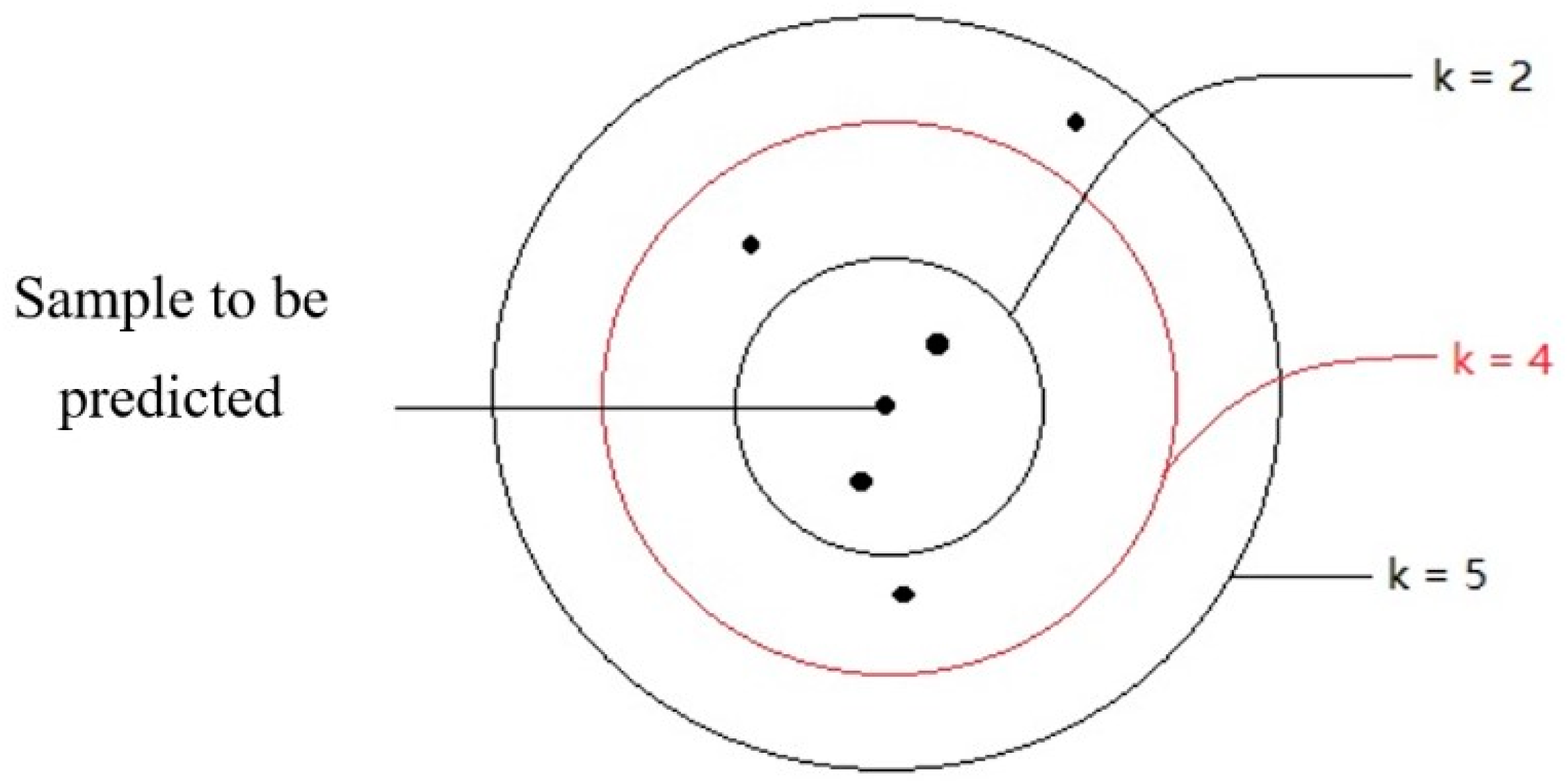
The K-Nearest Neighbor (KNN) algorithm is a simple and commonly used supervised learning method, and it was recognized as one of the top 10 algorithms [31]. KNN is mainly used for classification. Figure 1 shows a schematic diagram of KNN. The working principle of KNN is to find out the K training samples closest to a new test data point in the training set by using some distance measurement, and then to use the label of the K similar points to predict the test samples. In the progress of a regression, the average of the label values of the K sample is used as the prediction result. The weighted average can also be based on the distance, so the closer the sample weight is, the more accurate the prediction can be when the sample distribution is uneven. The advantage of the KNN algorithm the avoidance of the training process before classification. Instead of a training process, it simply saves the samples and calculates the distance after receiving the samples to be predicted [32]. On the other side of the coin, the time complexity of the prediction is large. In addition, the other main challenges in KNN include the computation of K, nearest neighbor selection, nearest neighbor search, and classification rule [33]. Despite these shortcomings, KNN is still an efficient artificial intelligence (AI) algorithm according to the comparison of 16 different algorithms by Li et al. [34].

As mentioned above, K is an important super-parameter in KNN, and it determines the precision of the prediction. The prediction results will be different when K takes different values. The computation of K relies on the sample’s distribution [35]. The selection of K can be based on either different sample subspaces [36] or different test samples [37]. Small ranges of training samples are used for prediction if a small K value is selected. In this way, the prediction error of KNN will be reduced if the sample size is large enough. This is because only the training samples close to the samples to be predicted play a role in the prediction results. Meanwhile, it is easier to overfit because the prediction results are very sensitive to adjacent samples. The prediction makes mistakes quite easily if an adjacent sample contains incorrect data. If a larger K value is selected, it is equivalent to using a wide range of samples for prediction. The advantage is that it can reduce the possibility of overfitting by the learner, but in this way, the training samples that are far away from the samples to be predicted will also play a role in prediction, resulting in a decline in the prediction accuracy. Generally, in practice, a K value with a smaller value is still selected. On the other hand, if different distance calculation methods are used, the “neighbors” found will be different, and the prediction results will, of course, be significantly different. The most commonly used distance measure is the $L_p$ distance or Minkowski distance.

2.2. Support Vector Regression Algorithm

Support Vector Regression (SVR) is also commonly accepted as one of the standard machine learning algorithms, and it falls under the category of supervised learning methods [38]. Its algorithmic principle can be summarized in the following two main points: (1) Firstly, it is a linear fitting algorithm that is only suitable for linearly distributed data. For data with a nonlinear distribution, a special nonlinear mapping is used to make their high-dimensional distribution linear, and the linear algorithm is used in the high-dimensional feature space to try to learn to fit the training data. (2) Secondly, the algorithm constructs an optimal hyperplane in the whole feature space based on the theory of structural risk minimization (including regularization). SVR is not a traditional regression fitting algorithm based on its basic principle. The main advantage of the SVR algorithm is the capability of achieving a global optimum and avoiding overfitting. The main feature of SVR comes from the different kernel functions that are used to fit different types of data. The computational complexity depends only on the number of support vectors. Therefore, a small number of support vectors determine the final result, not the entire dataset.

In the given training sample set $D=\{(x_1,y_1),(x_2,y_2),\dots \dots ,(x_m,y_m)\},yi\in R$, the objective is to have a regression model $f(x)={\omega }^{T}x+b$ that makes $f$ as close as possible to $y$. Both $\omega$ and $b$ are the model parameters that need to be determined. For a certain sample $(x,y)$, traditional regression models usually calculate the loss based on the difference between the model output $f(x)$ and the real value $y$. The loss is zero only when $f(x)$ and $y$ are exactly the same. In contrast, SVR can tolerate the maximum deviation between $f\left(x\right)$ and $y$. The loss is calculated only when the absolute value of the difference between $f(x)$ and $y$ is greater than $\epsilon$. The loss is not calculated for a sample with a prediction error falling to $\epsilon$, while the samples on and outside the spacer are called support vectors. Thus, the SVR problem can be written as:

$$\underset{\omega ,b}{\min }\frac{1}{2}{\Vert \omega \Vert }^2+C{\displaystyle \sum _{i=1}^m{l}_{\epsilon }}(f(x_i)-y_i)$$

(1)

where C is the regularization constant, which is a super-parameter; $l_{\epsilon }$ is the $\epsilon$− insensitive loss function, which can be determined with the following equation:

$$l_{\epsilon }=\left\{\begin{array}{ll}0,& if\left|z\right|\le \epsilon \\ \left|z\right|-\epsilon ,& otherwise\end{array}\right\}.$$

(2)

Introducing slack variables ${\xi }_i$ and ${\widehat{\xi }}_i$ and rewriting the above formula gives:

$$\begin{gathered} \underset{\omega ,b,{\xi }_i,{\widehat{\xi }}_i}{\min }\frac{1}{2}{\Vert \omega \Vert }^2+C{\displaystyle \sum _{i=1}^m({\xi }_i+{\widehat{\xi }}_i)} \\ \begin{array}{ll}s.t.& f(x_i)-y_i\le \epsilon +{\xi }_i\\ & yi-f(xi)\le \epsilon +{\widehat{\xi }}_i\\ & {\xi }_i\ge 0,{\widehat{\xi }}_i\ge 0,i=1,2,\dots ,m\end{array} \end{gathered}$$

(3)

After introducing the Lagrange multiplier ${\mu }_i\ge 0,{\widehat{\mu }}_i\ge 0,{\alpha }_i\ge 0,{\widehat{\alpha }}_i\ge 0$, the Lagrange function of Equation (3) can be obtained with the Lagrange multiplier method:

$$\begin{array}{l}L(\omega ,b,\alpha ,\widehat{\alpha },\xi ,\widehat{\xi },\mu ,\widehat{\mu })\\ =\frac{1}{2}{\Vert \omega \Vert }^2+C{\displaystyle \sum _{i=1}^m({\xi }_i+{\widehat{\xi }}_i)-{\displaystyle \sum _{i=1}^m{\mu }_i{\xi }_i}}-{\displaystyle \sum _{i=1}^m{\widehat{\mu }}_i{\widehat{\xi }}_i}\\ +{\displaystyle \sum _{i=1}^m{\alpha }_i(f(x_i)-y_i-\epsilon -{\xi }_i)}+{\displaystyle \sum _{i=1}^m{\widehat{\alpha }}_i(y_i-f(x_i)-\epsilon -{\widehat{\xi }}_i).}\end{array}$$

(4)

Let the partial derivative of $L(\omega ,b,\alpha ,\widehat{\alpha },\xi ,\widehat{\xi },\mu ,\widehat{\mu })$ to $\omega$, $b$, ${\xi }_i$, and ${\widehat{\xi }}_i$ be zero:

$$\omega ={\displaystyle \sum _{i=1}^m({\widehat{\alpha }}_i-{\alpha }_i)x_i}$$

(5)

$$0={\displaystyle \sum _{i=1}^m({\widehat{\alpha }}_i-{\alpha }_i)}$$

(6)

$$C={\alpha }_i+{\mu }_i$$

(7)

$$C={\widehat{\alpha }}_i+{\widehat{\mu }}_i$$

(8)

Substituting Equations (5)–(8) into Equation (4), the dual form of SVR can be obtained:

$$\begin{gathered} \begin{array}{cc}\hfill \underset{\alpha ,\widehat{\alpha }}{\max }& {\displaystyle \sum _{i=1}^m{y}_i({\widehat{\alpha }}_i-{\alpha }_i)-\epsilon ({\widehat{\alpha }}_i+{\alpha }_i)}\hfill \\ \hfill & -\frac{1}{2}{\displaystyle \sum _{i=1}^m{\displaystyle \sum _{j=1}^m({\widehat{\alpha }}_i-{\alpha }_i)({\widehat{\alpha }}_j-{\alpha }_j)x_i^T{x}_j}}\hfill \end{array} \\ \begin{array}{cc}s.t.& {\displaystyle \sum _{i=1}^m({\widehat{\alpha }}_i-{\alpha }_i)}=0,\\ & 0\le {\alpha }_i,{\widehat{\alpha }}_i\le C\end{array} \end{gathered}$$

(9)

Applying the Karush–Kuhn–Tucker (KKT) conditions when searching for the optimized value yields [39]:

$$\{\begin{array}{l}{\alpha }_i(f(x_i)-y_i-\epsilon -{\xi }_i)=0,\\ {\widehat{\alpha }}_i(y_i-f(x_i)-\epsilon -{\widehat{\xi }}_i)=0,\\ {\alpha }_i{\widehat{\alpha }}_i=0,{\xi }_i{\widehat{\xi }}_i=0,\\ (C-{\alpha }_i){\xi }_i=0,(C-{\widehat{\alpha }}_i){\widehat{\xi }}_i=0\end{array}.$$

(10)

Andreani et al. applied a sequential minimum optimization algorithm (SMO) to solve the above optimization problem [40]. Substituting Equation (5) into Equation (10), the solution of SVR is:

$$f(x)={\displaystyle \sum _{i=1}^m({\widehat{\alpha }}_i-{\alpha }_i)}{x}_i^{T}x+b.$$

(11)

According to the KKT conditions in Equation (10), the samples falling in the $\epsilon$−spacer satisfy ${\alpha }_i=0$ and ${\widehat{\alpha }}_i=0$. Therefore, the samples of $({\widehat{\alpha }}_i-{\alpha }_i)\ne 0$ in Equation (11) can be the support vector of SVR, which falls outside the $\epsilon$−spacing band. Obviously, the support vector of SVR is only a part of the training samples, and its solution is still sparse.

In addition, it can also be seen from the KKT conditions (Equation (10)) that $(C-{\alpha }_i){\xi }_i=0$ and ${\alpha }_i(f(x_i)-y_i-\epsilon -{\xi }_i)=0$ for each sample $(x_i,y_i)$. Therefore, after getting ${\alpha }_i$, it must be that ${\xi }_i=0$ for $0<{\alpha }_i<C$, which yields:

$$b=y_j+\epsilon -{\displaystyle \sum _{i=1}^m({\widehat{\alpha }}_i-{\alpha }_i)x_i^T{x}_j}.$$

(12)

In practical problems, multiple samples satisfying the condition $0<{\alpha }_i<C$ are often selected to solve b, and then the average is taken.

The sample is assumed to have a linear distribution in the above derivation; however, data are often nonlinear in real applications [41]. For such problems, the samples can be mapped from the original space to a higher-dimensional feature space so that they are linearly distributed in this new space.

Let $\varphi (x)$ denote the vector after mapping $x$ to a high-dimensional space, so the corresponding model of the linear regression equation in the new high-dimensional space is:

$$f(x)={\omega }^T\varphi (x)+b.$$

(13)

So, the solution of SVR is:

$$f(x)={\displaystyle \sum _{i=1}^m({\widehat{\alpha }}_i-{\alpha }_i)}\varphi {(x_i)}^T\varphi (x)+b$$

(14)

$$b=y_j+\epsilon -{\displaystyle \sum _{i=1}^m({\widehat{\alpha }}_i-{\alpha }_i)\varphi {(x_i)}^T\varphi (x_j)}.$$

(15)

However, there are still two problems: (1) Different data need different mapping functions $\varphi (x)$ for different scenarios, which makes it hard to predict how high the dimension at which the original sample is to be mapped should be to create a linear distribution. Therefore, the first problem comes from the selection of the mapping function $\varphi (x)$. (2) The solution involves the calculation of $\varphi {(x_i)}^T\varphi (x_j)$, which is the inner product of the sample $x_i$ and $x_j$ mapped to a high-dimensional space. Since the dimension may be very high or even infinite, a direct calculation is particularly difficult. A kernel function can help to solve these problems. Kernel functions show good performance in solving the optimization problems of increasing complexity [42,43]. In Equation (14), $\varphi {(x_i)}^T$ and $\varphi (x_j)$ always appear in pairs. Then, the following relationship can be derived:

$$\kappa (xi,xj)=\langle \varphi (x_i),\varphi (x_j)\rangle =\varphi {(x_i)}^T\varphi (x_j).$$

(16)

The inner product of $x_i$ and $x_j$ in a high--dimensional space is equal to the result calculated with the function $\kappa (x_i,x_j)$ in the original sample space. There is no need to pay attention to the selection of mapping functions with such a function. Therefore, the inner product in a high-dimensional or even infinite-dimensional feature space can be directly calculated, which involves mapping the input data into a higher-dimensional space [44]. The most commonly used kernel functions are shown in

Table 1. Commonly used kernel functions [44,45] (summarized from Daoud et al., and Bernal-de-Lázaro et al.).

Kernel	Expression	Comments
Linear Kernel	$\kappa \left(x_i,x_j\right)=x_i^T{x}_j$
Polynomial Kernel	$\kappa \left(x_i,x_j\right)={\left(x_i^T{x}_j\right)}^d$	$d\ge 1$, Number of polynomials
Gaussian Kernel	$\kappa \left(x_i,x_j\right)=\exp \left(-\frac{{\Vert x_i-x_j\Vert }^2}{2{\sigma }^2}\right)$	$\sigma >0$, Bandwidth of the Gaussian kernel
Sigmoid Kernel	$\kappa \left(x_i,x_j\right)=\tanh \left(\beta x_i^T{x}_j+\theta \right)$	tanh is a hyperbolic tangent function, β > 0, θ < 0

.

2.3. Boosting Tree Algorithm

Boosting is an integration method; within this category, the Boosting Tree is one of the most commonly used algorithms. The principle of ensemble learning is to learn repeatedly with a series of weak learners, which are later integrated into a strong learner to get better generalization performance [46]. As the name implies, the Lifting Tree is an algorithm that selects a weak learner as a decision tree and then integrates it. A weak learner is a machine learning model with performance that is a little better than that of chance. Some researchers used field datasets to prove that the Boosting Tree algorithm was better than a neural network algorithm [47]. The Boosting Tree mainly comprises two powerful algorithms, which are the Gradient Boosting Tree [48] and Extreme Gradient Boosting [49]. According to a case study provided by Tixier et al., the Gradient Boosting Tree (GBT) was proven to have better performance than that of other machine learning methods, since it can determine nonlinear and local relationships [50]. Extreme Gradient Boosting (XGB) is treated as an implementation of a Gradient Boosting Machine (GBM), but it is more accurate and efficient [51]. Some researchers also found that XGB algorithms could significantly reduce the risk of overfitting [52].

Given the training sample set $D=\{(x_1,y_1),(x_2,y_2),\dots \dots ,(x_N,y_N)\},yi\in R$, a regression tree corresponds to a partition of the input space and the output value on all partition units. Now, assuming that the space has been divided into $M$ units $R_1,R_2,\dots ,R_M$, and there is a fixed output value $c_m$ on each unit. The regression tree model can be expressed as:

$$f\left(x\right)={\displaystyle \sum _{m=1}^M{c}_{m}I\left(x\in R_m\right)}.$$

(17)

In machine learning, the square error is applied to represent the prediction error of the regression tree for the training data, and the minimum square error criterion is used to solve the optimal output value on each unit, which is transformed into an optimization problem [53]. The optimal value ${\widehat{c}}_m$ of $c_m$ on unit $R_m$ is the mean of output $y_i$ corresponding to all output instances $x_i$ on $R_m$:

$${\widehat{c}}_m=average\left(y_i|x_i\in R_m\right)$$

(18)

The jth feature of the data (x^(j)) and a certain value (or values) are assumed to be selected as the segmentation variable and segmentation point. Two regions are defined as follows:

$$R_1(j,s)=\left\{x|x^{(j)}\le s\right\} \mathrm{and} R_2(j,s)=\left\{x|x^{(j)}>s\right\}$$

(19)

Then, the optimal cut feature $j$ and the optimal cut point $s$ are found:

$$\underset{j,s}{\min }\left[\underset{c_1}{\min }{\displaystyle \sum _{x_i\in R_1\left(j,s\right)}{\left(y_i-c_1\right)}^2+\underset{c_2}{\min }{\displaystyle \sum _{x_i\in R_2\left(j,s\right)}{\left(y_i-c_2\right)}^2}}\right]$$

(20)

Traversing all features, the optimal segmentation features and optimal segmentation points are found. According to this rule, the input space is divided into two regions. Then, the above process is repeated for each region until the stop condition is satisfied, where a regression decision tree can be generated. Combining Equation (18) with (17), the final regression tree model is:

$$T\left(x;\theta \right)={\widehat{c}}_m\left(x\in R_m\right)$$

(21)

where the parameter $\theta =\{(R_1,{\widehat{c}}_1),(R_2,{\widehat{c}}_2),\dots ,(R_M,{\widehat{c}}_M)\}$ represents the regional division of the tree and the optimal value of each region; $M$ is the number of leaf nodes of the regression tree.

In the lifting tree, we use an additive model and a forward distribution algorithm. First, the initial lifting tree $f_0\left(x\right)=0$ is set, and the model in step t is:

$$f_t\left(x\right)=f_{t-1}\left(x\right)+T\left(x;{\theta }_t\right)$$

(22)

which is the current model $f_{t-1}(x)$. The required solution is:

$${\widehat{\theta }}_t=\arg \underset{{\theta }_t}{\min }{\displaystyle \sum _{i=1}^{N}L\left(y_i,f_{t-1}\left(x_i\right)+T\left(x_i;{\theta }_t\right)\right)}$$

(23)

The parameter ${\widehat{\theta }}_t$ of the t-tree is determined through empirical risk minimization.

When the square error loss function is used,

$$L\left(y,f\left(x\right)\right)={\left(y-f\left(x\right)\right)}^2$$

(24)

Then, the loss yields:

$$\begin{array}{ll}L\left(y,f_{t-1}\left(x\right)+T\left(x;{\theta }_t\right)\right)& ={\left(y-f_{t-1}\left(x\right)-T\left(x;{\theta }_t\right)\right)}^2\\ & ={\left(\gamma -T\left(x;{\theta }_t\right)\right)}^2\end{array}$$

(25)

Here, $\gamma$ is the residual of the predicted value of the t−1 tree:

$$\gamma =y-f_{t-1}\left(x\right)$$

(26)

So, the optimization goal of the t tree becomes:

$${\widehat{\theta }}_t=\arg \underset{{\theta }_t}{\min }{\displaystyle \sum _{i=1}^N{\left(\gamma -T\left(x_i;{\theta }_t\right)\right)}^2}$$

(27)

When the lifting tree solves the regression problem, it only needs to fit the residual of the predicted value of the previous tree. This means that the algorithm becomes quite simple, and the final model of the lifting tree can be expressed as an additive model.

$$f_T\left(x\right)={\displaystyle \sum _{t=1}^{T}T\left(x;{\theta }_t\right)}$$

(28)

where $T(x;{\theta }_t)$ represents the decision tree, ${\theta }_t$ is the parameter of the decision tree, and $T$ is the number of decision trees.

2.4. Multi-Layer Perceptron

The neural network is a representative algorithm in machine learning, and it is the most popular and widely used machine learning model [54]. A Multi-Layer Perceptron (MLP) is a supplement to feed-forward neural networks [55]. Similarly to a biological neural network, the most basic constituent unit of an artificial neural network is the ‘neuron’. Each neuron is connected to other neurons. It multiplies the weight on each edge and adds the bias of the neuron itself when it receives an input. The output of a neuron is finally generated through an activation function, which is a nonlinear function, such as a sigmoid function, arc-tangent function, or hyperbolic-tangent function [56]. A sigmoid function with many excellent properties is often selected as the most common activation function [57]. The perceptron model consists of two layers, which are the input layer and output layer. However, the perceptron has only two layers and only one output layer. One layer of functional neurons restricts the model to fitting data. To solve complex problems, multi-layer functional neurons are needed. The neuron layer between the input layer and the output layer is called the hidden layer. In other words, the Multi-Layer Perceptron (MLP) is a neural network model with multiple hidden layers. Each layer of neurons is completely connected to the next layer of neurons, and there are no connections within the same layer or cross-layer connections. Some researchers proved that a neural network with more than three layers could simulate any continuous function with arbitrary accuracy [58,59]. The learning of MLP takes place by adjusting the weights and biases between neurons according to the training data. An error back-propagation (BP) algorithm is commonly used to train multi-layer neural networks. These are based on a gradient descent strategy and are iterative optimization algorithms, which adjust the parameters in the negative gradient direction of the target parameters [60]. According to the gradient descent strategy, let the loss function be $f$ and a pair of parameters be $(\omega ,b)$. The initial values $({\omega }_0,b_0)$ are randomly selected; in the (n + 1)th iteration,

$${\omega }_{n+1}={\omega }_n-\alpha \frac{\partial f}{\partial \omega }|{}_{{\omega }_n,b_n}$$

(29)

$$b_{n+1}=b_n-\alpha \frac{\partial f}{\partial b}|{}_{{\omega }_n,b_n}$$

(30)

where the learning rate $\alpha \in (0,1)$ determines the update step size of each iteration of the algorithm. The oscillation causes the model to be unable to converge normally if the value of $\alpha$ is too large. The convergence speed of the algorithm is slow if too small of a value of $\alpha$ is used. The learning rate is usually set to 0.8 [60]. Newton’s method is applied for rapid convergence [61]. Then, Equations (29) and (30) yield:

$${\omega }_{n+1}={\omega }_n-{\left(\frac{{\partial }^{2}f}{\partial {\omega }^2}\right)}^{-1}\frac{\partial f}{\partial \omega }|{}_{{\omega }_n,b_n}$$

(31)

$$b_{n+1}=b_n-{\left(\frac{{\partial }^{2}f}{\partial b^2}\right)}^{-1}\frac{\partial f}{\partial b}|{}_{{\omega }_n,b_n}$$

(32)

Loss functions (or objective functions) may have multiple local extremums, but there is only one global minimum [62]. The global minimum value is the final objective of the calculations. However, for the gradient descent algorithm, in each iteration, the gradient of the loss function is calculated at a certain point, and then the optimal solution is determined along the negative gradient direction [63]. The gradient at the current point is zero if the loss function has reached the local minimum, where the updating of the parameters is terminated. This leads to a local extremum in the parameter optimization. The local minimum can be avoided through the following strategies in order to further approach the global minimum [64,65,66]: (1) The neural network is initialized with multiple sets of different parameters. The parameters with the loss function are the final solution after training. This process is equivalent to starting from multiple different initial points for optimization; then, we may fall into different local extremums, from which we can select the results closer to the global minimum. (2) The random gradient descent method is used. This method adds a random factor, and only one sample is used in each update. There will be a certain possibility of making the direction deviate from the optimal direction so that it can jump out of the local extremum.

2.5. Model Performance Evaluation

To evaluate machine learning models, several performance metrics are adopted and calculated to judge their performance. Based on case studies from other researchers, the mean absolute error (MAE) and coefficient of determination (R² Score) are often selected to evaluate the generalization ability of machine learning models [67]. The MAE is the average difference between the true value and the predicted values, and it can be easily calculated and compared. Some researchers even used some revised forms of the MAE, such as the dynamic mean absolute error and mean absolute percentage error, to evaluate the accuracy of a prediction model [68,69]. The more accurate the machine learning model is, the smaller the MAE will be. A perfect model causes the MAE to be close to 0. Let $f(x)$ and y denote the predicted value and the true value, respectively. Then, the MAE can be expressed as:

$$MAE=\frac{1}{m}{\displaystyle \sum _{i=1}^m\left|f\left(x_i\right)-y_i\right|}$$

(33)

The MAE can intuitively measure the ‘gap’ between the predicted value and the real value. However, it is difficult to compare a model’s effect when the equivalence dimensions are different.

Since the dimensions of different datasets are different, it is difficult to compare them by using a simple difference calculation. The coefficient of determination (R² Score) can be adopted to evaluate the degree of coincidence of the predicted values and true values [70]. Most recent research has proved the feasibility of using the R² Score to evaluate mixed-effect models, rather than just linear models [71]. The calculation of the R² Score involves three important performance judgment terms—the sum of squares for regression (SSR), sum of squares for error (SSE), and sum of squares for total (SST) [72]:

$$SST=SSR+SSE$$

(34)

Based on the above relationship, the calculation method for the R² Score can be defined as [73]:

$$R^2=1-\frac{{\sum }_i{\left(f\left(x_i\right)-y_i\right)}^2}{{\sum }_i{\left(\overline{y}-y_i\right)}^2}=1-\frac{MSE\left(f\left(x\right),y\right)}{Var\left(y\right)}=1-\frac{SSE}{SST}$$

(35)

where $MSE\left(f\left(x\right),y\right)$ is the mean square error between the predicted value $f\left(x\right)$ and the real value $y$; $Var\left(y\right)$ is the variance of the real value $y$. Specifically, there are the following situations in the analysis of the R² Score:

• If $R^2\approx 1$, the performance metric $MSE\left(f\left(x\right),y\right)$ is 0, indicating that the predicted label value in the test sample is exactly the same as the true value. A perfect model has been built to predict all of the test samples.
• If $R^2\approx 0$, the numerator is equal to the denominator, indicating that our predicted values are all the mean values of the real values. In this situation, the prediction model explains none of the variability of the response data around its mean. Sánchez et al. (2019) also explained that, in this scenario, the inclusion of variables can be neglected, and the built prediction model is not adequate [74].
• If $0<R^2<1$, the score is within the normal range. A value closer to 1 indicates a better fit, while a value closer to 0 indicates a worse fitting effect.
• For a bad scenario in which $R^2<0$, the numerator is greater than the denominator, that is, the error of the prediction data is greater than the variance of the real data. This indicates that the error of the predicted value is greater than the dispersion of the data, which indicates the misuse of a linear model for nonlinear data.

3. Prediction of Sand Production for an NGH Reservoir

3.1. Gravel-Filling Simulation Experiment

A sand control experiment was designed, as shown in Figure 2. The whole experimental process was carried out in a lab incubator to ensure safety. The key step when preparing the experiment was to make NGH reservoir samples under lab conditions. According to a survey of the literature, NGH samples for lab tests are mainly from field coring and lab preparation [74,75]. The field coring method is very costly because of the high requirements for temperature and pressure during transportation. In addition, some researchers have found that the physical properties of NGH samples obtained with the coring method may be changed in the sampling and transportation process [76]. Therefore, NGH samples were prepared in lab conditions. The NGH lab preparation method for the experiment was an in situ rapid preparation method that was proposed by Li et al. [77]. In the preparation, different sizes of produced sand (0.05 m³) were added into a reactor to simulate NGH reservoirs. The produced sand was mixed for a sand sieve analysis before being added into the reactor. The purpose was to present the effect of the uniformity coefficient (UC).

To simulate a real production process, several sand control screens were adopted in the experiment. The sand-retaining precision of the sand control screens was selected according to the preferred gravel mesh. An experiment was used to measure the actual sand production and sand content for the simulation experiment. Yu et al. [78]. designed experiments to show that the proper selection of the median diameter ratio of gravel can significantly reduce the risk of sand blockage in the exploitation and production of NGH. Therefore, the selection of the precision of gravel packing was vital in both the experiment and in field sand control. The criterion for the selection of the median gravel size was obtained with Saucier’s method, with a gravel size of 5~6 × d₅₀.

The purpose of the experiment was to use the changing variables as the independent variable x and the measured sand production as the label y to establish a machine learning model. The experiment contained eight characteristics: the well type, permeability (md), shale content (%), sand diameter d₅₀ (mm), effective porosity (%), hydrate saturation (%), sand-retaining precision (the diameter of the mesh screen, mm), and uniformity coefficient (d₄₀/d₉₀); sand production (g) was used as a label value.

Table 2. Original data from the experiment.

	d1	d2	d3	d4	d5	d6	d7	d8	y
x1	Horizontal Pipe	510.7	22.5	0.23	24.2	31.9	0.177	3.42	0.31
x2	Horizontal well	48.6	28.2	0.236	16	43.7	0.125	3.353	0.19
x3	Vertical Pipe	494.7	21.7	0.236	22.1	41.4	0.149	3.353	0.22
x4	Vertical Pipe	617.9	12	0.236	21.6	41.4	0.177	3.353	0.27
x5	Vertical Pipe	93.2	20.9	0.236	15.9	41.4	0.125	3.353	0.15
x6	Horizontal Pipe	863.7	9.7	0.31	22.4	41.4	0.21	5.34	0.31
x7	Horizontal Pipe	1047.6	7	0.252	23.02	41.4	0.177	3.27	0.22
x8	Horizontal Pipe	233	15.3	0.194	10.6	58.0	0.177	2.17	0.48
x9	Vertical Pipe	107.7	14.6	0.161	22.7	46.7	0.149	3.17	0.45
x10	Horizontal Pipe	442.4	0.9	0.237	22.4	35.3	0.21	2.85	0.51
x11	Horizontal Pipe	452.3	9.3	0.217	32.3	23.5	0.177	2.303	0.21
x12	Horizontal Pipe	452.3	16.8	0.289	31.8	16.3	0.177	1.897	0.41
x13	Vertical Pipe	452.3	13.9	0.203	26.6	55.5	0.149	1.854	0.42
x14	Vertical Pipe	452.3	0.1	0.19	29.7	61.5	0.149	1.876	0.4
x15	Horizontal Pipe	838.3	8.8	0.27	25.8	41.4	0.25	5.68	1.21
x16	Horizontal Pipe	130.3	12.5	0.283	21.2	41.4	0.297	6.4	1.32

illustrates the measured values, where x_i represents the ith dataset, $d_i$ represents the above features, and $y$ represents the label value of sand production.

3.2. Modeling with Different Machine Learning Algorithms

3.2.1. Feature Selection and Data Pre-Processing

Feature selection is the first and vital step in the process of modeling with machine learning. Proper feature selection can improve a machine learning model’s performance by reducing overfitting and the curse of dimensionality [79]. For processes with large amounts of data, feature selection has been shown to have a positive role in increasing the calculation efficiency [80]. The main step in feature selection is the reduction of the feature numbers by checking if a parameter is irrelevant or redundant [81]. Scatter diagrams of each feature $d_i$ and label $y$ were drawn (Figure 3, Figure 4, Figure 5, Figure 6, Figure 7, Figure 8, Figure 9 and Figure 10), which aimed at analyzing the impact of each feature on the label value. Figure 3 roughly explains the effect of the well type. The scatter plot (Figure 3) shows the effects of well types on sand production. In addition, more significant sand production was observed in the horizontal well compared to that in the vertical well. This relationship was verified by some other researchers, such as Sparlin and Shang et al., who found that sand production was severe with long horizontal sections [82,83]. Figure 4 shows the relationship between permeability and sand production. Generally, the various permeability values caused different sand production levels, as was also seen in previous research [84,85]. It was concluded that permeability was an effective but not very significant feature in sand production. The effectiveness was because the scatter points were concentrated in the middle and on the left side of the graph, while the “not that significant” characterization came from the still two points located on the right side. Figure 5 illustrates that the effect of the shale content had the same trend as that of the effect of permeability on sand production. The scatter points in Figure 5 are slightly more concentrated than those of permeability in Figure 4. The preliminary assessment showed that the median size of the produced sand was more relevant than the shale content (Figure 6). As shown in Figure 7, the effective porosity was more obviously relevant to sand production compared to the other parameters. Previous studies explained that porosity could significantly affect sand production as a main transportation path for flowing sand [86,87,88]. Based on the scatter points in Figure 8, the hydrate saturation was less relevant to sand production compared to the porosity. Fang et al. designed experiments to investigate the sand production behavior in an NGH sediment. In the above experiments, the free sand mainly came from the dissociation of the hydrate, which caused the saturation to affect sand production through the phase change [89]. Saturation could be treated as an indirect factor by considering the changes in pressure and temperature. The pressure and temperature were fixed in this experiment, which explained the lower relevance of saturation as a feature to the output label value. The concentrated distributions of points in Figure 9 and Figure 10 prove the high relevance of sand-retaining precision and the uniformity coefficient, respectively, to sand production.

To summarize Figure 3, Figure 4, Figure 5, Figure 6, Figure 7, Figure 8, Figure 9 and Figure 10, it seemed to be easier to produce more sand with horizontal wells than with vertical wells. Wells with low permeability produced sand easily. A large effective porosity value increased the amount of sand produced. A small uniformity coefficient increased the sand risk. It was found that not all features had a simple linear relationship with the label value. Based on this perception, a nonlinear algorithm was adopted to fit the features. It must also be noted that there were two data points outside the system for all features, which may have been for two reasons: (1) These were two noise points coming from experimental error, and they should be abandoned; (2) the coverage of the collected data was not wide enough. There were many data points between these two outliers, and there were other data that were not collected. Since the amount of data collected in this paper was small, the second reason could explain why the two points seemed to be outliers.

The above scatter plots helped to intuitively and briefly show the relevance of each feature to the output label. For a quantifiable verification, the correlations between features were analyzed by using the correlation coefficients between them (as shown in

Table 3. Correlation coefficients between features.

	d2	d3	d4	d5	d6	d7	d8
d2	1	−0.4673	0.426423	0.377929	−0.13718	0.259615	0.170625
d3	−0.4673	1	0.009319	−0.41641	−0.15977	−0.39754	0.015433
d4	0.426423	0.009319	1	0.108746	−0.50727	0.565289	0.612933
d5	0.377929	−0.41641	0.108746	1	−0.43826	0.110464	−0.19554
d6	−0.13718	−0.15977	−0.50727	−0.43826	1	−0.1836	−0.05787
d7	0.259615	−0.39754	0.565289	0.110464	−0.1836	1	0.730236
d8	0.170625	0.015433	0.612933	−0.19554	−0.05787	0.730236	1

). The correlation coefficient is a special and important covariance that eliminates the influence of dimension [90]. The closer the value is to 1, the more obvious the trend of positive correlation between features is. On the other side of the coin, the closer the value is to −1, the more obvious the trend of negative correlation between features is. A weaker the correlation is found if the correlation coefficient gets closer to 0.

It was obvious that there were strong positive correlations between sand-retaining accuracy and uniformity coefficient, as well as between the median sand diameter and uniformity coefficient. This could be explained by the fact that the definition of the uniformity coefficient was highly related to the median value of particle size. A greater value for these features meant that a higher sand-retaining accuracy was required for sand production, which validated the accuracy of the experimental results. According to Table 3, there were no strong correlations between features on the whole. Since the number of features was not very large, feature extraction methods, such as principal component analysis, were not suitable for the data [91]. Random forest has the advantages of high accuracy and good robustness [92]. The fitting effect of the nonlinear relationship was also good, and there was no need for much debugging. The random forest method was used for feature selection in this study. The base learner used 100 decision trees. The importance of each feature in the random forests is shown in Figure 11.

As shown in Figure 11, the uniformity coefficient and sand-retaining precision were the two most important characteristics, the total importance of which exceeded 80%. According to the characteristics of the random forest, the values of the contribution of other features will decrease rapidly when one feature is selected. Therefore, the high importance values of the uniformity coefficient and sand-retaining precision did not mean that the other features were dispensable; however, it could provide a reference for the selection of features. The top four features were chosen to train the model; these were the uniformity coefficient, sand-retaining precision, effective porosity, and permeability. These four features are also consistent with the professional knowledge of sand control. The four features were selected and standardized with a standardized formula (Equation (36)). The standardized data could eliminate the influence of each feature dimension. Furthermore, they helped to avoid the interference of the model prediction without changing the distribution of the data themselves [93].

$${\widehat{x}}_i=\frac{x_i-mean\left(x\right)}{std\left(x\right)}$$

(36)

where $x_i$ represents the original data; $mean(x)$ is the mean of the feature; $std(x)$ is the standard deviation of the feature. The standardized data are shown in

Table 4. Standardized data for model training.

	d2	d5	d7	d8	y
x1	0.21	0.21	−0.06	0.05	0.31
x2	−1.43	−1.27	−1.26	0.01	0.19
x3	0.15	−0.17	−0.7	0.01	0.22
x4	0.59	−0.26	−0.06	0.01	0.27
x5	−1.28	−1.29	−1.26	0.01	0.15
x6	1.46	−0.11	0.7	1.5	0.31
x7	2.11	0.01	−0.06	−0.06	0.22
x8	−0.78	−2.24	−0.06	−0.89	0.48
x9	−1.22	−0.06	−0.7	−0.14	0.45
x10	−0.04	−0.11	0.7	−0.38	0.51
x11	0.01	1.68	−0.06	−0.79	0.21
x12	0.01	1.58	−0.06	−1.1	0.41
x13	0.01	0.65	−0.7	−1.13	0.42
x14	0.01	1.21	−0.7	−1.12	0.4
x15	1.37	0.5	1.61	1.76	1.21
x16	−1.14	−0.33	2.69	2.3	1.32

.

3.2.2. Training and Testing

The pseudo-code for the KNN Algorithm 1 is shown below.

Algorithm 1. KNN pseudo-code.

# Importing the necessary libraries

# Read files to input pre-processed data and labels

Input original training data: train.csv

Input k

For i in training data

Distance (Euclidean) = square root of (sum of (point i2 − point i + 12))

Sort Distance

#Make Prediction;

For i in training data

Predict Point Distance i = square root of (sum of (test point2 − train point i2))

Determine the minimum Predict Distance

Predicted value = mean of minimum Predict Distance

The pseudo-code for the SVR Algorithm 2 is shown below.

Algorithm 2. SVR pseudo-code.

# Importing the necessary libraries

# Read files to input pre-processed data and labels

Input original training data: train.csv

# Calculate parameters w, b

For j = 1 in the training dataset

b = average [yj-sum(Lagrangian multiplier*yj*xj)]

w = sum(Lagrangian multiplier**yj*xj)

Check KKT conditions (continuing if satisfied)

Define Kernel Function (linear, sigmoid, polynomial, gaussian)

Assume d = 1

For i = 1 in the test dataset

Y_predicted = sign(sum(Lagrangian multiplier*x_test*Kernel Function + b

The pseudo-code for the Boosting Tree (XGBoost) Algorithm 3 is shown below.

Algorithm 3. XGBoost pseudo-code.

# Importing the necessary libraries

# Read files to input pre-processed data and labels

Input original training data: train.csv

Input parameters I, d

Initial gain = 0

Define Gi = Sum of gi (i is the example number), Hj = Sum of hj (j is the nod number)

For i = 1

Initial predict value = 0, G1 = 0, H1 = 0

Predict Yi = Predict Yi – 1 + New Regression Function*Shrinkage

Objective function = Sum [(Predict Value-True Value)2] + Regularization Term

Determine the optimum w by minimizing objective function

Predict Y = 1/2*sum($\frac{G^2}{H+Complexity}$) + Complexity*Node Number

The pseudo-code for the Multi-Layer Perceptron Algorithm 4 is shown below.

Algorithm 4. MLP pseudo-code.

# Importing the necessary libraries

# Read files to input pre-processed data and labels

Input original training data: train.csv

Input parameters w, b, n

For l = n − 1 to 1

For i in the training set

Y_predict_i = wixi + bi

Cost function_i = (Y_predict_i-Y_true)*Sigmoid function(Y_predict_i)

Back-propagation algorithm to calculate Cost Function_l with dw and db

Obtain New w, b

Calculate loss function = 1/2*sum(Y_predict − Y_true)2

Determine the minimum loss function

The pseudo-code for model performance is shown below (Algorithm 5).

Algorithm 5. MSE and R2 pseudo-code. (* means times itself).

#Calculate Accuracy (MSE & R2)

for row in range(0,actual_class_array_size):

Squared_Error = (abs((actual_array[row] − predicted_array[row])))

Squared_Error * = Squared_Error

Squared_Error_Array[row] = Squared_Error

MSE = mean(squared_error_array)

R2_Score = 1 − MSE/var(actual_array[row])

End

The data in Table 4 were randomly split into the training set and test set according to the ratio of 7:3, namely, there were 11 training samples and 5 test samples. After training the model with the training set, the MAE and R² Score on the test set were calculated for the model. The final optimized model would be built after fully tuning the parameters. To avoid contingency, we randomly divided all of the data six times, which meant repeating the above process six times and observing the results. The results are shown in

Table 5. Results of the modeling assessment.

	First Training		Second Training		Third Training		Fourth Training		Fifth Training		Sixth Training
	MAE	R2	MAE	R2	MAE	R2	MAE	R2	MAE	R2	MAE	R2
KNN	0.20	0.56	0.08	−0.03	0.26	0.33	0.20	0.58	0.08	0.30	0.19	0.57
SVR	0.13	0.86	0.11	−0.50	0.13	0.84	0.11	0.87	0.11	−0.23	0.08	0.96
Boosting Tree	0.09	0.94	0.07	0.30	0.10	0.92	0.08	0.94	0.08	−0.29	0.08	0.97
MLP	0.09	0.92	0.11	−0.65	0.13	0.86	0.09	0.91	0.11	−0.42	0.12	0.88

and Figure 12, Figure 13, Figure 14, Figure 15, Figure 16, Figure 17, Figure 18, Figure 19, Figure 20, Figure 21, Figure 22 and Figure 23.

It could be seen that the R² Scores of the second and fifth training were negative, while the other R² Scores were positive. In addition, the values of MAE from the second and fifth training were very close to those of other models. This indicated that the proposed model had no problem in itself. Focusing on the training set and test set after dividing the data each time, it was found that the second and fifth times divided the two outliers into the training set, leading to two problems: (1) The outlier data were used in training, but the test set did not have similar samples to predict, which led to large errors in the model predictions. (2) There were no outliers in the test set, but the number of samples was small, resulting in the concentration of the label value of y and a decrease in the variance. This made the R² Score smaller and even negative. In other partitions, the two outliers were divided into the training set and test set so that the values were normal. Based on the above analysis, the second and fifth R² Scores were excluded when calculating the average performance of the model, as shown in

Table 6. Average scores in the evaluation of model performance.

	MAE	R2 Score
KNN	0.17	0.51
SVR	0.11	0.88
Boosting Tree	0.08	0.94
MLP	0.11	0.89

and Figure 24 and Figure 25.

As shown in Figure 12, Figure 13, Figure 14, Figure 15, Figure 16, Figure 17, Figure 18, Figure 19, Figure 20, Figure 21, Figure 22 and Figure 23, each algorithm could fit the training set well. Even though the fitting effect of SVR was slightly insufficient compared to those of the other algorithms, it still could help to learn the overall trend of data. Based on the training performance, the second modeling and the fifth modeling performed poorly. The reason for the poor performance was discussed in the previous section; it was mainly because the amount of data was not large enough to cover a large sample space, and some samples, such as outliers, were not fully learned.

Figure 24 and Figure 25 show that the best generalization model was the Boosting Tree (XGBoost), while the worst was KNN. SVR and MLP had similar performances. KNN predicted the new samples according to the adjacent samples in its space. This would require a large sample size, and the samples should be evenly distributed in the feature space. The sample size in this paper was small and the feature space was ‘sparse’, which decreased the algorithm’s performance. The Boosting Tree is an integrated learning method that can be regarded as an additive model, and it is based on a residual learning mechanism. It did not require too many calculations and did not have the problem of overfitting, making it very excellent in this paper. SVR and MLP had many parameters, and they were also able to show good performance when the parameters were adjusted properly. The two algorithms had a very strong fitting ability for nonlinear data and very good performance in the data processing used in this paper.

3.2.3. Tuning and Discussion

Based on the above training and testing, the Boosting Tree had the best performance in the prediction of sand production. SVR and MLP had the second best performance based on the MSE and R² Score. One of the current popular applications of machine learning is to build an ensemble machine learning model to increase the performance and accuracy of prediction, classification, and clustering [94,95,96]. The main feature of ensemble machine learning models is the building of a coupled model with different machine learning algorithms. The final result of an ensemble machine learning model is determined by voting with the built-in algorithms, and it is the most accurate model in a specific scenario [97]. An ensemble machine learning model is built based on the important knowledge that different algorithms have their own proper scenarios, causing the ensemble model to significantly reduce the variance [98,99,100]. Therefore, the Boosting Tree (XGBoost), SVR, and MLP should all be discussed in this study, rather than only focusing on the best algorithm.

The main parameter in the SVR algorithm is the type of kernel function. Table 1 shows the common kernel functions, including the linear kernel, polynomial kernel, Gaussian kernel, and sigmoid kernel, which were all tested in the paper. The linear kernel is the simplest of all of the kernel functions. The linear kernel function is determined by the sum of the inner product of the training and true values (x,y) and an optional constant c [101]. The polynomial kernel function is a non-stationary kernel, which works well for normalized training data [102]. The Gaussian kernel is a radial basis function [103]. Some researchers, such as Lin et al., pointed out that, as a radial basis function, the Gaussian kernel was better than the sigmoid kernel [104]. The tuning process in this paper also compared the prediction performance when using different kernel functions (Figure 26). It could be seen that the Gaussian kernel had a low MSE and high R² Score. Therefore, the Gaussian kernel was recommended in the model for the prediction of sand production based on the SVR algorithm.

The main parameters of XGBoost were tested in the proper range, which was similar to those used by Pan et al. and Parsa; the ranges are shown in the following table (

Table 7. Ranges of parameters in the tuning process of the XGBoost algorithm.

Parameter	Range	Type
Maximum Depth of Tree	[4, 7] with a step of 1	Integer
Gamma	[0, 4] with a step of 0.2	Floating
Sampling Rate of Training Sample	[0.7, 1.0] with a step of 0.05	Floating
Regular Term of Weight L1	[0, 0.3] with a step of 0.05	Floating
Regular Term of Weight L2	[0, 0.3] with a step of 0.05	Floating

) [105,106]. The tuning results are illustrated in Figure 27, Figure 28, Figure 29, Figure 30 and Figure 31. Figure 27 proves that the proper value of the maximum depth of tree was around 5, with a low MAE and high R² Score. According to Figure 28, the recommended value of gamma was around 1 in order to achieve a proper MSE and R² Score. Figure 29 shows that the sampling rate of the training sample should be 0.9 for a low MSE and a high R² Score at the same time. The tuning process also found that both the regular term of weight L1 and regular term of weight L2 had little effect on the prediction performance (Figure 30 and Figure 31).

The number of hidden layers in the MLP algorithm is usually recommended to be two in some case studies [107]. The main parameter for MLP tuning was the node number of the hidden layer. The potential range of the node number was [10,38] with a step of 1. Figure 32 illustrates the tuning results for the node number. It was shown that the proper node number for the hidden layer was 14 (Figure 32).

3.3. Case Study with Machine Learning Algorithms

This paper also involved one case study in order to validate the model and to show the application potential of the proposed model. The case study compared the results of the numerical simulation and those of the proposed model with machine learning algorithms. Uchida et al. built a mathematical model to predict sand production by investigating sand migration [23]. The results of the comparison are shown in Figure 33. The training data were selected at every 6 h in the interval of the 2nd day to the 7th day in Uchida’s results. It was concluded that the three machine algorithms (SVR, XGBoost, MLP) performed well and could match most of the simulation results, especially at the stable-pressure stage. The main drawback of the machine learning algorithms was displayed in the early stage of sand production. There were still some gaps between the results of the simulation and the machine learning predictions. However, it should be noticed that the XGBoost algorithm provided more matching results compared to the other two machine learning algorithms. The case study’s results also supported the point that XGBoost could provide the most accurate results among the three algorithms. The case study also validated the feasibility of applying machine learning in the prediction of sand production.

4. Conclusions

The comparison of four machine learning algorithms for application to laboratory-scale sand production tests revealed the following results:

(1)

This paper built a machine learning model to predict the sand production in an unconsolidated NGH reservoir with four different algorithms, which were KNN, SVR, Boosting Tree (XGBoost), and MLP. The input data for the model were provided by a sand production experiment.

(2)

As shown by the comparison of the four different algorithms, KNN had the worst performance, while XGBoost provided prediction results with the lowest MSE value and a high R² Score. The final algorithms selected for building further ensemble models were SVR, XGBoost, and MLP.

(3)

The tuning process showed that the kernel function had a great impact on the performance of SVR. The kernel function recommended for the sand prediction model was the Gaussian kernel. The best parameters for the XGBoost algorithm were tested and provided; these included the maximum depth of tree, gamma, sampling rate of the training sample, regular term of weight L1, and regular term of weight L2.

(4)

The three selected machine learning algorithms were also applied to the results of a rigorous numerical simulation (Uchida et al., 2016), and all of them were able to give results that reasonably matched with those of the numerical solution. XGBoost performed better and was recommended for the prediction of sand production in the early sand production stage.

References

1. Boswell, R.; Collett, T.S. Current perspectives on gas hydrate resources. Energy Environ. Sci. 2010, 4, 1206–1215. [Google Scholar] [CrossRef]
2. Li, X.-S.; Xu, C.-G.; Zhang, Y.; Ruan, X.-K.; Li, G.; Wang, Y. Investigation into gas production from natural gas hydrate: A review. Appl. Energy 2016, 172, 286–322. [Google Scholar] [CrossRef]
3. Guerin, G.; Goldberg, D. Sonic waveform attenuation in gas hydrate-bearing sediments from the Mallik 2L-38 research well, Mackenzie Delta, Canada. J. Geophys. Res. Earth Surf. 2002, 107, EPM-1. [Google Scholar] [CrossRef]
4. Yamamoto, K. Overview and introduction: Pressure core-sampling and analyses in the 2012–2013 MH21 offshore test of gas production from methane hydrates in the eastern Nankai Trough. Mar. Pet. Geol. 2015, 66, 296–309. [Google Scholar] [CrossRef]
5. Heeschen, K.U.; Abendroth, S.; Priegnitz, M.; Spangenberg, E.; Thaler, J.; Schicks, J.M. Gas Production from Methane Hydrate: A Laboratory Simulation of the Multistage Depressurization Test in Mallik, Northwest Territories, Canada. Energy Fuels 2016, 30, 6210–6219. [Google Scholar] [CrossRef]
6. Tamaki, M.; Fujii, T.; Suzuki, K. Characterization and Prediction of the Gas Hydrate Reservoir at the Second Offshore Gas Production Test Site in the Eastern Nankai Trough, Japan. Energies 2017, 10, 1678. [Google Scholar] [CrossRef]
7. Li, F.; Yuan, Q.; Li, T.; Li, Z.; Sun, C.; Chen, G. A review: Enhanced recovery of natural gas hydrate reservoirs. Chin. J. Chem. Eng. 2019, 27, 2062–2073. [Google Scholar] [CrossRef]
8. Zhao, J.; Liu, Y.; Guo, X.; Wei, R.; Yu, T.; Xu, L.; Sun, L.; Yang, L. Gas production behavior from hydrate-bearing fine natural sediments through optimized step-wise depressurization. Appl. Energy 2020, 260, 114275. [Google Scholar] [CrossRef]
9. Li, Z.; Han, J. Environmental safety and low velocity of the development of submarine natural gas hydrate with examples of test production in South China Sea. Environ. Sci. Pollut. Res. 2021, 28, 6259–6265. [Google Scholar] [CrossRef]
10. Zhu, H.; Xu, T.; Yuan, Y.; Xia, Y.; Xin, X. Numerical investigation of the natural gas hydrate production tests in the Nankai Trough by incorporating sand migration. Appl. Energy 2020, 275, 115384. [Google Scholar] [CrossRef]
11. Kvamme, B.; Coffin, R.; Wei, N.; Zhou, S.; Zhao, J.; Li, Q.; Saeidi, N.; Chien, Y.-C.; Dunn-Rankin, D.; Sun, W.; et al. Stages in Dynamics of Hydrate Formation and Consequences for Design of Experiments for Hydrate Formation in Sediments. Energies 2019, 12, 3399. [Google Scholar] [CrossRef]
12. Yan, C.; Li, Y.; Cheng, Y.; Wang, W.; Song, B.; Deng, F.; Feng, Y. Sand production evaluation during gas production from natural gas hydrates. J. Nat. Gas Sci. Eng. 2018, 57, 77–88. [Google Scholar] [CrossRef]
13. Deng, J.; Li, P.; Wang, L.; He, B.; Zhao, W. The optimization of sand control method for moderate sand control technique application in Bohai Bay. Oil Drill. Prod. Technol. 2011, 33, 98–101. [Google Scholar] [CrossRef]
14. Deng, F.; Feng, Y.; Yan, C.; Lin, H.; Gong, N.; Wang, J. Experimental investigation of factors affecting gravel pack efficiency for thermal recovery wells in Bohai Bay, China. J. Pet. Sci. Eng. 2017, 156, 835–844. [Google Scholar] [CrossRef]
15. Kurihara, M.; Sato, A.; Funatsu, K.; Ouchi, H.; Yamamoto, K.; Numasawa, M.; Ebinuma, T.; Narita, H.; Masuda, Y.; Dallimore, S.R.; et al. Analysis of Production Data for 2007/2008 Mallik Gas Hydrate Production Tests in Canada. In Proceedings of the International Oil and Gas Conference and Exhibition in China, Beijing, China, 8–10 June 2010. [Google Scholar] [CrossRef]
16. Terao, Y.; Duncan, M.; Hay, B.; Dang, L. Deepwater Methane Hydrate Gravel Packing Completion Results and Challenges. In Proceedings of the Offshore Technology Conference, Houston, TX, USA, 5–8 May 2014. [Google Scholar] [CrossRef]
17. Li, Y.L.; Liu, C.L.; Liu, L.L.; Huang, M.; Meng, Q.G. Triaxial shear test and strain analysis of unconsolidated hydrate-bearing sediments. Nat. Gas Geosci. 2017, 28, 383–390. [Google Scholar] [CrossRef]
18. Zhu, Y.; Wang, H.; Chen, C.; Luo, T. Effects of sand contents on mechanical characteristics of methane hydrate-bearing sediments in the permafrost. J. Nat. Gas Sci. Eng. 2020, 75, 103129. [Google Scholar] [CrossRef]
19. Zhang, Y.; Zhang, Y. The Numerical Analysis of Elastic Visco-Plastic Biot’S Consolidation to Marine Soft Soil. J. Jilin Univ. Earth Sci. Ed. 2003, 33, 71–75. [Google Scholar] [CrossRef]
20. Wu, E.L.; Wei, C.F.; Wei, H.Z. A statistical damage constitutive model of hydrate-bearing sediments. Rock Soil Mech. 2013, 34, 60–65. [Google Scholar] [CrossRef]
21. Wang, R.; Zhang, L.; Sun, H.; Liu, T.; Ning, F.; Jiang, G. Progress in Key Technologies Hydrate Cores from for Handling Natural Gas Ocean Sedi-ments. Geol. Sci. Technol. Inf. 2017, 36, 249–257. [Google Scholar] [CrossRef]
22. He, J.; Jiang, M. Macro-micro mechanical property of pore-filling type methane hydrate-bearing sediment in true triaxial tests based on distinct element analysis. Rock Soil Mech. 2016, 37, 3026–3034. [Google Scholar] [CrossRef]
23. Uchida, S.; Klar, A.; Yamamoto, K. Sand production model in gas hydrate-bearing sediments. Int. J. Rock Mech. Min. Sci. 2016, 86, 303–316. [Google Scholar] [CrossRef]
24. Ataie-Ashtiani, B.; Shobeyri, G. Numerical simulation of landslide impulsive waves by incompressible smoothed particle hydrodynamics. Int. J. Numer. Methods Fluids 2008, 56, 209–232. [Google Scholar] [CrossRef]
25. Chang, X.; Yuan, X. Application of strength reduction method considering hydromechanical coupling to analyze anti-sliding stability of gravity dams. Eng. J. Wuhan Univ. 2012, 45, 545–549. [Google Scholar]
26. Taoufik, N.; Boumya, W.; Achak, M.; Chennouk, H.; Dewil, R.; Barka, N. The state of art on the prediction of efficiency and modeling of the processes of pollutants removal based on machine learning. Sci. Total Environ. 2022, 807, 150554. [Google Scholar] [CrossRef] [PubMed]
27. Sarkar, S.; Vinay, S.; Raj, R.; Maiti, J.; Mitra, P. Application of optimized machine learning techniques for prediction of occupational accidents. Comput. Oper. Res. 2019, 106, 210–224. [Google Scholar] [CrossRef]
28. Zhou, S.; Wang, S.; Wu, Q.; Azim, R.; Li, W. Predicting potential miRNA-disease associations by combining gradient boosting decision tree with logistic regression. Comput. Biol. Chem. 2020, 85, 107200. [Google Scholar] [CrossRef]
29. Sutton, C.D. Classification and Regression Trees, Bagging, and Boosting. In Handbook of Statistics; Rao, C.R., Wegman, E.J., Solka, J.L., Eds.; Elsevier: Amsterdam, The Netherlands, 2005; Volume 24, pp. 303–329. [Google Scholar] [CrossRef]
30. Desai, M.; Shah, M. An anatomization on breast cancer detection and diagnosis employing multi-layer perceptron neural network (MLP) and Convolutional neural network (CNN). Clin. eHealth 2021, 4, 1–11. [Google Scholar] [CrossRef]
31. Wu, X.; Kumar, V.; Quinlan, J.R.; Ghosh, J.; Yang, Q.; Motoda, H.; McLachlan, G.J.; Ng, A.; Liu, B.; Philip, S.Y.; et al. Introduction to Network Analysis of Microwave Circuits. In Software VNA and Microwave Network Design and Characterisation; John Wiley & Sons, Ltd.: Hoboken, NJ, USA, 2008; Volume 14, pp. 1–37. [Google Scholar] [CrossRef]
32. Zhang, S.; Cheng, D.; Deng, Z.; Zong, M.; Deng, X. A novel k NN algorithm with data-driven k parameter computation. Pattern Recognit. Lett. 2018, 109, 44–54. [Google Scholar] [CrossRef]
33. Zhang, S. Challenges in KNN Classification. IEEE Trans. Knowl. Data Eng. 2021, 1. [Google Scholar] [CrossRef]
34. Li, W.; Zhang, Y.; Sun, Y.; Wang, W.; Li, M.; Zhang, W.; Lin, X. Approximate Nearest Neighbor Search on High Dimensional Data—Experiments, Analyses, and Improvement. IEEE Trans. Knowl. Data Eng. 2019, 32, 1475–1488. [Google Scholar] [CrossRef]
35. Tan, M.; Zhang, S.; Wu, L. Mutual kNN based spectral clustering. Neural Comput. Appl. 2020, 32, 6435–6442. [Google Scholar] [CrossRef]
36. Zhang, S.; Zhang, J.; Zhu, X.; Qin, Y.; Zhang, C. Missing Value Imputation Based on Data Clustering. In Transactions on Computational Science I; Springer: Berlin/Heidelber, Germany, 2008; pp. 128–138. [Google Scholar] [CrossRef]
37. Zhang, S.; Li, X.; Zong, M.; Zhu, X.; Cheng, D. Learning k for kNN Classification. ACM Trans. Intell. Syst. Technol. 2017, 8, 1–19. [Google Scholar] [CrossRef]
38. Cristianini, N.; Campbell, C.; Shawe-Taylor, J. Multiplicative Updatings for Support Vector Learning; NeuroCOLT Technical Report NC-TR-98-016; Royal Holloway College: Egham, UK, 1998. [Google Scholar]
39. Wu, H.-C. The Karush–Kuhn–Tucker optimality conditions in multiobjective programming problems with interval-valued objective functions. Eur. J. Oper. Res. 2009, 196, 49–60. [Google Scholar] [CrossRef]
40. Andreani, R.; Haeser, G.; Martínez, J.M. On sequential optimality conditions for smooth constrained optimization. Optimization 2011, 60, 627–641. [Google Scholar] [CrossRef]
41. Nie, F.; Zhu, W.; Li, X. Decision Tree SVM: An extension of linear SVM for non-linear classification. Neurocomputing 2020, 401, 153–159. [Google Scholar] [CrossRef]
42. Motai, Y. Kernel Association for Classification and Prediction: A Survey. IEEE Trans. Neural Netw. Learn. Syst. 2014, 26, 208–223. [Google Scholar] [CrossRef]
43. Ge, Z.; Song, Z.; Ding, S.X.; Huang, B. Data Mining and Analytics in the Process Industry: The Role of Machine Learning. IEEE Access 2017, 5, 20590–20616. [Google Scholar] [CrossRef]
44. Bernal-De-Lázaro, J.M.; Cruz-Corona, C.; Silva-Neto, A.J.; Llanes-Santiago, O. Criteria for optimizing kernel methods in fault monitoring process: A survey. ISA Trans. 2022, 127, 259–272. [Google Scholar] [CrossRef]
45. Al Daoud, E.; Turabieh, H. New empirical nonparametric kernels for support vector machine classification. Appl. Soft Comput. 2013, 13, 1759–1765. [Google Scholar] [CrossRef]
46. Oyedele, A.; Ajayi, A.; Oyedele, L.O.; Delgado, J.M.D.; Akanbi, L.; Akinade, O.; Owolabi, H.; Bilal, M. Deep learning and Boosted trees for injuries prediction in power infrastructure projects. Appl. Soft Comput. 2021, 110, 107587. [Google Scholar] [CrossRef]
47. Callens, A.; Morichon, D.; Abadie, S.; Delpey, M.; Liquet, B. Using Random forest and Gradient boosting trees to improve wave forecast at a specific location. Appl. Ocean Res. 2020, 104, 102339. [Google Scholar] [CrossRef]
48. Greenwell, B.; Boehmke, B.; Cunningham, J. Gbm: Generalized Boosted Regression Models. R Package Version 2.1.5, 2019, 1–39. Available online: https://cran.r-project.org/web/packages/gbm/index.html (accessed on 15 July 2020).
49. Chen, T.; He, T.; Benesty, M.; Khotilovich, V.; Tang, Y.; Cho, H.; Chen, K.; Mitchell, R.; Cano, I.; Zhou, T. Xgboost: Extreme Gradient Boosting. R Package Version 1.0.0.2, 2020, 1–57. Available online: https://cran.r-project.org/web/packages/xgboost/xgboost.pdf (accessed on 16 April 2022).
50. Tixier, A.J.-P.; Hallowell, M.R.; Rajagopalan, B.; Bowman, D. Application of machine learning to construction injury prediction. Autom. Constr. 2016, 69, 102–114. [Google Scholar] [CrossRef]
51. Sheridan, R.P.; Wang, W.M.; Liaw, A.; Ma, J.; Gifford, E.M. Extreme Gradient Boosting as a Method for Quantitative Structure–Activity Relationships. J. Chem. Inf. Model. 2016, 56, 2353–2360. [Google Scholar] [CrossRef]
52. Fan, J.; Wang, X.; Wu, L.; Zhou, H.; Zhang, F.; Yu, X.; Lu, X.; Xiang, Y. Comparison of Support Vector Machine and Extreme Gradient Boosting for predicting daily global solar radiation using temperature and precipitation in humid subtropical climates: A case study in China. Energy Convers. Manag. 2018, 164, 102–111. [Google Scholar] [CrossRef]
53. Sigrist, F. KTBoost: Combined Kernel and Tree Boosting. Neural Process. Lett. 2021, 53, 1147–1160. [Google Scholar] [CrossRef]
54. Sainlez, M.; Heyen, G. Recurrent neural network prediction of steam production in a Kraft recovery boiler. In Computer Aided Chemical Engineering; Pistikopoulos, E.N., Georgiadis, M.C., Kokossis, A.C., Eds.; Elsevier: Amsterdam, The Netherlands, 2011; Volume 29, pp. 1784–1788. [Google Scholar] [CrossRef]
55. Leng, J.; Wang, D.; Shen, W.; Li, X.; Liu, Q.; Chen, X. Digital twins-based smart manufacturing system design in Industry 4.0: A review. J. Manuf. Syst. 2021, 60, 119–137. [Google Scholar] [CrossRef]
56. Theodoridis, S. Chapter 18—Neural Networks and Deep Learning. In Machine Learning, 2nd ed.; Academic Press: London, UK, 2020; pp. 901–1038. [Google Scholar] [CrossRef]
57. Bakr, M.H.; Negm, M.H. Chapter Three—Modeling and Design of High-Frequency Structures Using Artificial Neural Networks and Space Mapping. In Advances in Imaging and Electron Physics; Jamal Deen, M., Ed.; Elsevier: Amsterdam, The Netherlands, 2012; Volume 174, pp. 223–260. [Google Scholar] [CrossRef]
58. Li, Z.; Li, H. Study on Communication Jamming Effects Evaluation Using the Artificial Neural Network. Ship Electron. Eng. 2005, 25, 109–112. [Google Scholar]
59. Wang, J. Research on BP Neural Network Theory and Its Application in Agricultural Mechanization. Ph.D. Thesis, Shenyang Agricultural University, Shenyang, China, June 2011. [Google Scholar]
60. Davies, E.R. Chapter 25—Biologically Inspired Recognition Schemes. In Signal Processing and Its Applications, Machine Vision, 3rd ed.; Morgan Kaufmann Publishers: Burlington, MA, USA, 2005; pp. 725–755. [Google Scholar] [CrossRef]
61. Rebentrost, P.; Schuld, M.; Wossnig, L.; Petruccione, F.; Lloyd, S. Quantum gradient descent and Newton’s method for constrained polynomial optimization. New J. Phys. 2019, 21, 073023. [Google Scholar] [CrossRef]
62. Couso, I.; Sánchez, L. Machine learning models, epistemic set-valued data and generalized loss functions: An encompassing approach. Inf. Sci. 2016, 358–359, 129–150. [Google Scholar] [CrossRef]
63. Steinwart, I. How to Compare Different Loss Functions and Their Risks. Constr. Approx. 2007, 26, 225–287. [Google Scholar] [CrossRef]
64. Feizi, S.; Javadi, H.; Zhang, J.; Tse, D. Porcupine Neural Networks: (Almost) All Local Optima are Global. arXiv 2017, arXiv:1710.02196. [Google Scholar]
65. Dominico, G.; Parpinelli, R.S. Multiple global optima location using differential evolution, clustering, and local search. Appl. Soft Comput. 2021, 108, 107448. [Google Scholar] [CrossRef]
66. Kafka, D.; Wilke, D.N. An empirical study into finding optima in stochastic optimization of neural networks. Inf. Sci. 2021, 560, 235–255. [Google Scholar] [CrossRef]
67. Wu, C.; Shen, H.; Shen, A.; Deng, J.; Gan, M.; Zhu, J.; Xu, H.; Wang, K. Comparison of machine-learning methods for above-ground biomass estimation based on Landsat imagery. J. Appl. Remote Sens. 2016, 10, 35010. [Google Scholar] [CrossRef]
68. Frías-Paredes, L.; Mallor, F.; Gastón-Romeo, M.; León, T. Dynamic mean absolute error as new measure for assessing forecasting errors. Energy Convers. Manag. 2018, 162, 176–188. [Google Scholar] [CrossRef]
69. McKenzie, J. Mean absolute percentage error and bias in economic forecasting. Econ. Lett. 2011, 113, 259–262. [Google Scholar] [CrossRef]
70. Xu, X.; Li, B. Study on the influence of different explained variable selection on determination coefficient R2 (Chinese). J. Taiyuan Univ. Sci. Technol. 2007, 28, 363–365. [Google Scholar]
71. Zhang, D. Coefficients of Determination for Mixed-Effects Models. arXiv 2021, arXiv:1710.02196. [Google Scholar]
72. Sánchez, A.R.; Gómez, R.S.; García, C. The coefficient of determination in the ridge regression. Commun. Stat.—Simul. Comput. 2019, 51, 201–219. [Google Scholar] [CrossRef]
73. Ives, A.R. R2s for correlated data: Phylogenetic models, LMMs, and GLMMs. Syst. Biol. 2019, 68, 234–251. [Google Scholar] [CrossRef]
74. Abid, K.; Spagnoli, G.; Teodoriu, C.; Falcone, G. Review of pressure coring systems for offshore gas hydrates research. Underw. Technol. 2015, 33, 19–30. [Google Scholar] [CrossRef]
75. Liu, C.; Li, Y.; Sun, J.; Wu, N. Gas hydrate production test: From experimental simulation to field practice. Mar. Geol. Quat. Geol. 2017, 37, 12–26. [Google Scholar] [CrossRef]
76. Waite, W.F.; Kneafsey, T.; Winters, W.J.; Mason, D.H. Physical property changes in hydrate-bearing sediment due to depressurization and subsequent repressurization. J. Geophys. Res. Earth Surf. 2008, 113, B07102. [Google Scholar] [CrossRef]
77. Li, H.; Zhao, J.; Liu, A.; Zhang, L.; Wei, N.; Wu, K.; Zhou, S.; Pei, J.; Zhang, W.; Yang, L.; et al. Experiment and evaluation on the in-situ rapid preparation of marine non-diagenetic natural gas hydrate. Nat. Gas Ind. B 2020, 7, 93–100. [Google Scholar] [CrossRef]
78. Yu, T. Experimental Study on the Behavior and Micro Mechanism of Sand Production during Hydrate Exploitation. Master’s Thesis, Dalian University of Technology, Dalian, China, June 2020. [Google Scholar] [CrossRef]
79. Alsahaf, A.; Petkov, N.; Shenoy, V.; Azzopardi, G. A framework for feature selection through boosting. Expert Syst. Appl. 2022, 187, 115895. [Google Scholar] [CrossRef]
80. Borboudakis, G.; Tsamardinos, I. Forward-Backward Selection with Early Dropping. J. Mach. Learn. Res. 2019, 20, 1–39. [Google Scholar]
81. Bolón-Canedo, V.; Alonso-Betanzos, A. Ensembles for feature selection: A review and future trends. Inf. Fusion 2019, 52, 1–12. [Google Scholar] [CrossRef]
82. Sparlin, D. Sand Control in Horizontal Wells. World Oil, August 2005, pp. 77–80. Available online: https://www.worldoil.com/magazine/2005/august-2005/features/sand-control-in-horizontal-wells (accessed on 15 July 2020).
83. Shang, J.; Zhu, C.; Luo, S.; Zhu, P.; Wang, W.; Yang, Z. Application of sand production technology in horizontal well to find leak stuck seal in Bohai oilfield. China Pet. Chem. Stand.Qual. 2019, 39, 245–247. (In Chinese) [Google Scholar]
84. Zeng, X.; He, G.; Sun, F.; Wang, P. Influences of sand production on permeability and experiments on sand production characters in SZ36-1 Oilfield. Pet. Explor. Dev. 2005, 32, 105–108. [Google Scholar] [CrossRef]
85. Xie, Y. Study on Permeability Variation Near Well of Moderate Sand Production Well in Unconsolidated Sandstone Reservoir. Ph.D. Thesis, Southwest Petroleum University, Chengdu, China, 2017. [Google Scholar]
86. Teng, F. Simulation Experiment on Sand Production from Gas Hydrate Reservoir. Master’s Thesis, China University of Petroleum, Dongying, China, 2018. [Google Scholar]
87. Yu, T.; Liu, Y.; Song, Y. Experimental study on sand production characteristics in natural gas hydrate deposits. IOP Conf. Ser. Earth Environ. Sci. 2020, 446, 052056. [Google Scholar] [CrossRef]
88. Guo, M.; Liu, H.; Wang, Y.; Zhang, H.; Wang, J.; Dong, X. Sand production by hydraulic erosion during multicycle steam stimulation: An analytical study. J. Pet. Sci. Eng. 2021, 201, 108424. [Google Scholar] [CrossRef]
89. Fang, X.; Ning, F.; Wang, L.; Liu, Z.; Lu, H.; Yu, Y.; Li, Y.; Sun, J.; Shi, H.; Zhao, Y.; et al. Dynamic coupling responses and sand production behavior of gas hydrate-bearing sediments during depressurization: An experimental study. J. Pet. Sci. Eng. 2021, 201, 108506. [Google Scholar] [CrossRef]
90. Filho, A.D.S.; Zebende, G.; de Castro, A.; Guedes, E. Statistical test for Multiple Detrended Cross-Correlation Coefficient. Phys. A Stat. Mech. Appl. 2021, 562, 125285. [Google Scholar] [CrossRef]
91. Karimi, A.M.; Sadeghnejad, S.; Rezghi, M. Well-to-well correlation and identifying lithological boundaries by principal component analysis of well-logs. Comput. Geosci. 2021, 157, 104942. [Google Scholar] [CrossRef]
92. Hong, Y.; Chen, S.; Chen, Y.; Linderman, M.; Mouazen, A.M.; Liu, Y.; Guo, L.; Yu, L.; Liu, Y.; Cheng, H.; et al. Comparing laboratory and airborne hyperspectral data for the estimation and mapping of topsoil organic carbon: Feature selection coupled with random forest. Soil Tillage Res. 2020, 199, 104589. [Google Scholar] [CrossRef]
93. Riaboff, L.; Aubin, S.; Bédère, N.; Couvreur, S.; Madouasse, A.; Goumand, E.; Chauvin, A.; Plantier, G. Evaluation of pre-processing methods for the prediction of cattle behaviour from accelerometer data. Comput. Electron. Agric. 2019, 165, 104961. [Google Scholar] [CrossRef]
94. Gangula, R.; Thirupathi, L.; Parupati, R.; Sreeveda, K.; Gattoju, S. Ensemble machine learning based prediction of dengue disease with performance and accuracy elevation patterns. Mater. Today Proc. 2021; in press. [Google Scholar] [CrossRef]
95. Olabanjo, O.A.; Aribisala, B.S.; Mazzara, M.; Wusu, A.S. An ensemble machine learning model for the prediction of danger zones: Towards a global counter-terrorism. Soft Comput. Lett. 2021, 3, 100020. [Google Scholar] [CrossRef]
96. Jain, S.; Saha, A. Improving performance with hybrid feature selection and ensemble machine learning techniques for code smell detection. Sci. Comput. Program. 2021, 212, 102713. [Google Scholar] [CrossRef]
97. Wang, C.W. New Ensemble Machine Learning Method for Classification and Prediction on Gene Expression Data. In Proceedings of the 28th IEEE EMBS Annual International Conference, New York, NY, USA, 30 August–3 September 2006. [Google Scholar] [CrossRef]
98. Breiman, L. Bagging predictors. Mach. Learn. 1996, 24, 123–140. [Google Scholar] [CrossRef]
99. Lam, L.; Suen, S. Application of majority voting to pattern recognition: An analysis of its behavior and performance. IEEE Trans. Syst. Man Cybern.—Part A Syst. Hum. 1997, 27, 553–568. [Google Scholar] [CrossRef]
100. Dietterich, T.G. Ensemble Methods in Machine Learning. In Proceedings of the International Workshop on Multiple Classifier Systems, Cagliari, Italy, 9–11 June 2000; pp. 1–15. [Google Scholar] [CrossRef]
101. Yang, J.; Li, Y.; Tian, Y.; Duan, L.; Gao, W. A new multiple kernel approach for visual concept learning. In Advances in Multimedia Modeling, Proceedings of the 15th International Multimedia Modeling Conference, LNCS, Kyoto, Japan, 9–11 January 2008; Springer: Berlin/Heidelberg, Germany, 2009; Volume 5371, pp. 250–262. [Google Scholar] [CrossRef]
102. Hofmann, T.; Schölkopf, B.; Smola, A.J. Kernel methods in machine learning. Ann. Stat. 2008, 36, 1171–1220. [Google Scholar] [CrossRef]
103. Zhang, L.; Zhou, W.; Jiao, L. Wavelet support vector machine. IEEE Trans. Syst. Man Cybern. Part B Cybern. 2004, 34, 34–39. [Google Scholar] [CrossRef] [PubMed]
104. Lin, H.; Lin, C. A Study on Sigmoid Kernels for SVM and the Training of nonPSD Kernels by SMO-Type Methods; Technical Report; Department of Computer Science, National Taiwan University: Taipei, Taiwan, 2003. [Google Scholar] [CrossRef]
105. Pan, S.; Zheng, Z.; Guo, Z.; Luo, H. An optimized XGBoost method for predicting reservoir porosity using petrophysical logs. J. Pet. Sci. Eng. 2022, 208, 109520. [Google Scholar] [CrossRef]
106. Parsa, M. A data augmentation approach to XGboost-based mineral potential mapping: An example of carbonate-hosted Zn Pb mineral systems of Western Iran. J. Geochem. Explor. 2021, 228, 106811. [Google Scholar] [CrossRef]
107. Taki, M.; Rohani, A.; Soheili-Fard, F.; Abdeshahi, A. Assessment of energy consumption and modeling of output energy for wheat production by neural network (MLP and RBF) and Gaussian process regression (GPR) models. J. Clean. Prod. 2018, 172, 3028–3041. [Google Scholar] [CrossRef]
Figure 1. Schematic diagram of KNN (the circle represents an isometric line).
Energies 15 06509 g001
Figure 2. Experimental device for the simulation of sand production.
Energies 15 06509 g002
Figure 3. Well type and measured sand production.
Energies 15 06509 g003
Figure 4. Permeability and measured sand production.
Energies 15 06509 g004
Figure 5. Shale content and measured sand production.
Energies 15 06509 g005
Figure 6. Median sand diameter and measured sand production.
Energies 15 06509 g006
Figure 7. Effective porosity and measured sand production.
Energies 15 06509 g007
Figure 8. Hydrate saturation and measured sand production.
Energies 15 06509 g008
Figure 9. Sand-retaining precision and measured sand production.
Energies 15 06509 g009
Figure 10. Uniformity coefficient and measured sand production.
Energies 15 06509 g010
Figure 11. Importance of features calculated by the random forest.
Energies 15 06509 g011
Figure 12. Results of the first training with training dataset.
Energies 15 06509 g012
Figure 13. Assessment of the first training with the test dataset.
Energies 15 06509 g013
Figure 14. Results of the second training with the training dataset.
Energies 15 06509 g014
Figure 15. Assessment of the second training with the test dataset.
Energies 15 06509 g015
Figure 16. Results of the third training with the training dataset.
Energies 15 06509 g016
Figure 17. Assessment of the third training with the test dataset.
Energies 15 06509 g017
Figure 18. Results of the fourth training with the training dataset.
Energies 15 06509 g018
Figure 19. Assessment of the fourth training with the test dataset.
Energies 15 06509 g019
Figure 20. Results of the fifth training with the training dataset.
Energies 15 06509 g020
Figure 21. Assessment of the fifth training with the test dataset.
Energies 15 06509 g021
Figure 22. Results of the sixth training with the training dataset.
Energies 15 06509 g022
Figure 23. Assessment of the sixth training with the test dataset.
Energies 15 06509 g023
Figure 24. Comparison of the different algorithms based on the MAE.
Energies 15 06509 g024
Figure 25. Comparison of the different algorithms based on the R2 Score.
Energies 15 06509 g025
Figure 26. Tuning results of different kernel functions for the SVR algorithm.
Energies 15 06509 g026
Figure 27. Tuning results for the maximum depth of tree.
Energies 15 06509 g027
Figure 28. Tuning results for gamma.
Energies 15 06509 g028
Figure 29. Tuning results for the sampling rate of the training sample.
Energies 15 06509 g029
Figure 30. Tuning results for the regular term of weight L1.
Energies 15 06509 g030
Figure 31. Tuning results for the regular term of weight L2.
Energies 15 06509 g031
Figure 32. Tuning results for the node number for the hidden layer.
Energies 15 06509 g032
Figure 33. Comparison between the numerical results from Uchida [23] and those of the machine learning algorithms.
Energies 15 06509 g033