Article

Numerical Analysis of Aeroacoustic Characteristics around a Cylinder under Constant Amplitude Oscillation

1
School of Aeronautics, Northwestern Polytechnical University, Xi’an 710072, China
2
Unmanned System Research Institute, Northwestern Polytechnical University, Xi’an 710129, China
*
Author to whom correspondence should be addressed.
Energies 2022, 15(18), 6507; https://doi.org/10.3390/en15186507
Submission received: 6 June 2022 / Revised: 29 July 2022 / Accepted: 18 August 2022 / Published: 6 September 2022

Abstract

:
The present study numerically investigated a cylinder under oscillating motions at a low Reynolds number. The effects of two oscillation frequencies and amplitudes on the lift drag coefficient, near-field surface pressure fluctuation, and far-field noise were studied. The models were examined at a Mach number of 0.05, corresponding to a Reynolds number of 1.0 × 10⁵. In this paper, the incompressible Navier–Stokes equations (INSE) and linearized perturbed compressible equations (LPCE) were coupled to form a hybrid noise prediction method, which was used to solve the flow field and acoustic radiation field. Based on the simulation results of the acoustic radiation field, the frequency characteristics of the acoustic waves were analyzed by the dynamic modal decomposition (DMD) method. It was observed that when the oscillation amplitude was the same, the variation amplitude and mean value of the lift-drag coefficient increased with the increase in the oscillation frequency. Under the same small oscillation frequency, the oscillation amplitude had little effect on the lift-drag coefficient. However, for the same large oscillation frequency, the variation amplitude of the lift-drag coefficient increased as the oscillation amplitude increased. In addition, both the amplitude and frequency had a significant effect on the directionality of the noise and the intensity of the sound waves. The main energy of the sound field was mainly concentrated on the first and second narrowband frequencies by using the DMD method to analyze the sound pressure level spectrum.

1. Introduction

In recent years, with the wide application of micro air vehicles (MAVs) in military and civil fields such as reconnaissance, monitoring, communication, etc., aerodynamics and aeroacoustics at low Reynolds numbers ( Re = 10 3 10 5 ) have become one of the research hotspots. The maneuvering flight of a MAV usually experiences unstable states such as pitching and heaving oscillation. As a simplified model of MAV, the flows of the cylinder or airfoil offer an opportunity to study the basic underlying physics of flow phenomena. Research [1,2] has found that under the same incoming flow conditions, the flow field structure and aerodynamic noise characteristics induced by the oscillating bluff body are quite different from those induced by the static bluff body.
At present, many wind tunnel experiments and numerical simulations have been carried out on the aerodynamic characteristics of the oscillating bluff body. For instance, Kumar et al. [3] experimentally studied the phenomenon of vortex shedding in a rotationally oscillating cylinder at a Reynolds number of 185. It was found that the phenomenon of lock-on occurs in a forcing frequency range, which depends not only on the amplitude of oscillation but also on the downstream location from the cylinder. Soumarup et al. [4] also carried out experimental studies on oscillating cylinders at low Reynolds numbers ( Re = 190 and Re = 250 ) and reached similar conclusions to Kumar et al. In addition, Amiralaei et al. [5] conducted relevant experiments on oscillating airfoil tests in the range of 555~5000 Reynolds numbers. The results showed that motion parameters such as the decreasing frequency and amplitude of oscillation have a great influence on the strength of the vortex structure near the airfoil, and thus affect the aerodynamic characteristics. Most of the aerodynamic experiments on oscillating cylinders or airfoils have been conducted at low Reynolds numbers ( Re = 10 2 10 3 ), and the flow field characteristics of medium Reynolds numbers ( Re = 10 4 10 5 ) have been studied by numerical simulation. For example, Tuncer and Platzer [6] carried out a numerical simulation of the oscillating airfoil under Reynolds numbers of 10,000 and 100,000 and analyzed the wake vortex structure formation, separation characteristics, average aerodynamic force, and propulsion efficiency under different flapping amplitude and frequency. Miyanawala et al. [7], Nagarajan et al. [8], and others have also carried out relevant numerical simulations.
The acoustic problem of the oscillating blunt body has been a research hotspot in recent years, and many scholars have carried out related acoustic experiments. For instance, an experimental investigation on the acoustic far field of a thin elastic airfoil, immersed in a low-Mach non-uniform stream flow, was examined by Manela [9]. The results showed that the structure elasticity and pitching frequency are relevant to the sound intensity of a pitching airfoil. The trailing-edge noise from a pitching airfoil at a low Reynolds number was conducted by Zhou et al. [10]. It was revealed that a high-level narrow-band noise hump occurred at a specific angle of attack in a pitching cycle. In one pitching period, the moment when the narrow-band noise hump occurs is independent of the pitching amplitude and is delayed as the pitching frequency increases. Subsequently, Zhou T. et al. [11] conducted an experimental study on the far-field noise and near-field flow characteristics of the heaving NACA0012 airfoil in the anechoic wind tunnel. The corresponding conclusions were also verified in the experiments of Zhang B. [12], Mayer Y. [13], Siegel [14], and Zajamsek [15] et al. Although many conclusions can be obtained from the acoustic experiments of the oscillating blunt body, it is difficult to intuitively obtain the acoustic characteristics of the whole space field and sound wave propagation process, which is unfavorable for the mechanism analysis of noise. In the numerical simulation of aeroacoustics of the oscillating bluff body, scholars at home and abroad have also produced some excellent research results. Taking a transversely oscillating cylinder in a uniform flow as a model, Zheng et al. [16] investigated the effects of oscillation frequency on lift, drag, and far-field pressure fluctuations. The far-field pressure is calculated by the formula based on the Curleintegral method. The trailing-edge noise of a flat plate at a free stream Mach number of 0.6 and a Reynolds number of 12,000 based on the boundary layer thickness at the inflow boundary was investigated by Seong [17] using large-eddy simulations (LES) and solutions of the acoustic perturbation equations [18]. Guo et al. [19] applied a computational fluid dynamics (CFD) solver and Lighthill’s acoustic analogy to analyze the flow field and induced the sound field characteristics of the oscillating airfoil, respectively. However, few have summarized the influence of different frequencies and amplitudes on the aerodynamic and acoustic characteristics in these conclusions. In addition, computational aeroacoustic (CAA) numerical simulation methods are mostly based on acoustic analogy methods, so it is difficult to directly observe the spatial noise intensity distribution and sound wave propagation process.
Therefore, it is both interesting and timely to investigate the aerodynamic and aeroacoustic behaviors of an oscillating bluff body at different oscillation frequencies and amplitudes by using the high-precision hybrid INSE/LPCE method. The framework of the article is mainly divided into the following six sections. The introduction reviews the research progress in aerodynamics and aeroacoustics of oscillating airfoils or cylinders by scholars both at home and abroad. Section 2 mainly introduces the theory and implementation strategy of the hybrid CFD/CAA method. In Section 3, taking an oscillating cylinder as an object, the reliability of the numerical method is verified by comparing the calculated results with the experimental data. In Section 4, the calculation conditions of oscillating cylinders with different frequencies and the setting of the calculation grid are given. Section 5 mainly analyzes the aerodynamic and aeroacoustics characteristics of oscillating cylinders, reveals the noise generation mechanism, and summarizes the relevant conclusions.

2. Numerical Method

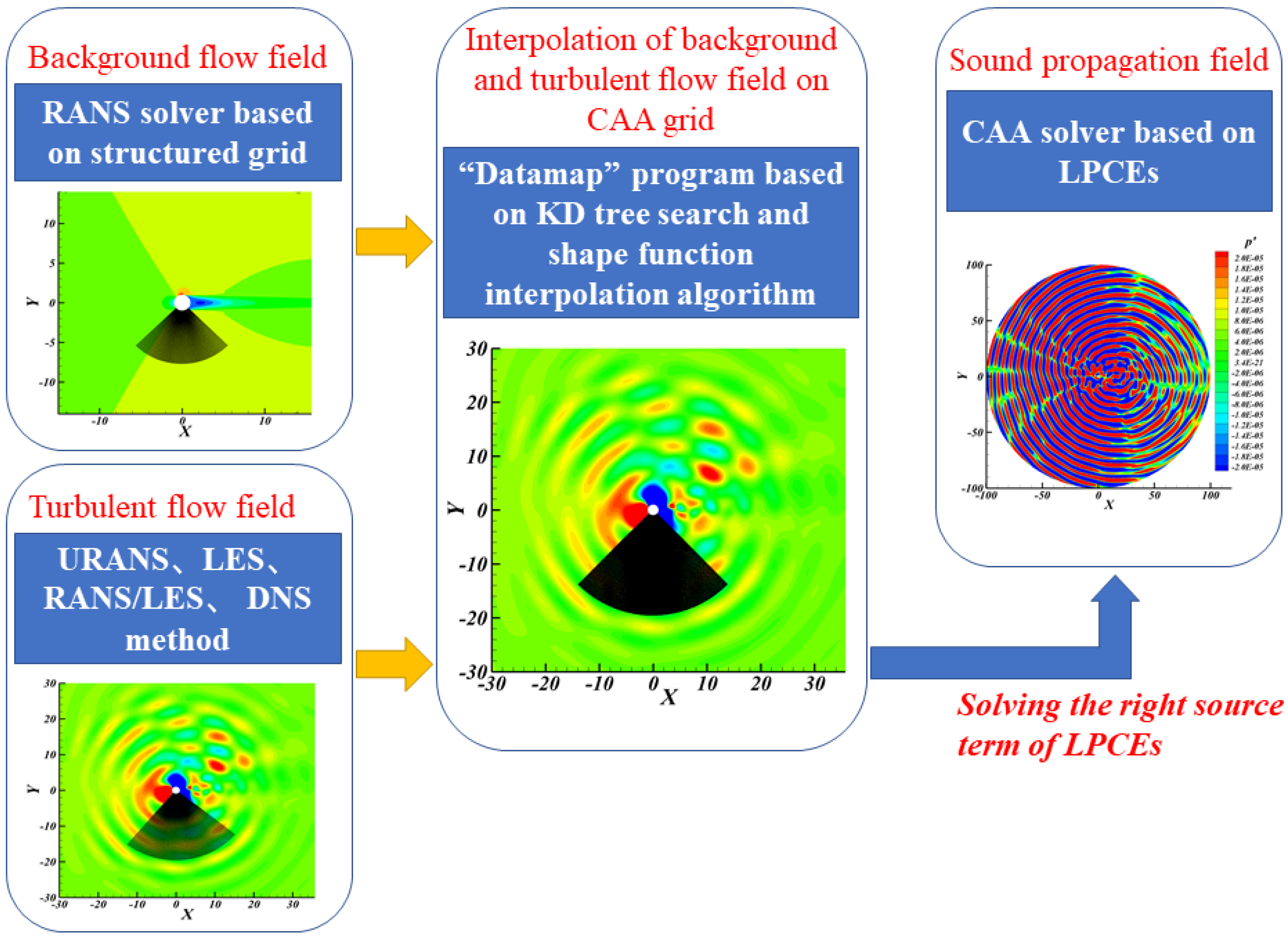
2.1. Governing Equations for Hybrid CAA Method

2.1.1. CFD Solver

To provide a reliable aerodynamic noise source for oscillating cylinders, we adopted an open-source incompressible/compressible CFD code “cfl3d” on the website (http://cfl3d.larc.nasa.gov, accessed on 4 September 2021). For the CFD calculation of incompressible fluid, the Weiss–Smith preprocessing method is used to modify the computational stability of Navier–Stokes equations. In a curvilinear coordinate system, its non-dimensionless two-dimensional form is shown in the following expression:
I i n c t Q J + ξ 1 J F ξ x + G ξ y + η 1 J F η x + G η y = 0
in which
I i n c = Ω 0 0 ρ T 0 ρ 0 0 0 0 ρ 0 1 0 0 ρ C p
ρ , u , v , p , and T are the density, velocity component, pressure, and temperature of the fluid. Ω is given by
Ω = 1 U r 2 ρ T ρ C p
where ρ T = ρ / T p ; C P is the specific heat at constant pressure. U r is a reference velocity. The specific definition of variable U r can be found in [20].
A coordinate transformation between Cartesian and curvilinear coordinates is applied in the calculation. The variable J represents the Jacobian of the transformation:
J = ξ , η , t x , y , t
where Q = p , u , v , T T . F and G are flux terms in two directions of the Cartesian coordinate system. The convection terms are discretized by Roe’s upwind-difference scheme. A second-order accurate Monotone Upstream-centered Scheme for Conservation Laws (MUSCL) was employed to determine the interpolation accuracy of the state-variable on the cell interfaces. The shear stress and heat transfer terms were discretized by the central difference scheme.
To update the flow variables on the grid nodes caused by the rotation of the cylinder, a hybrid mesh deformation method combining radial basis function (RBF) and transfinite interpolation (TFI) was adopted. The RBF method can obtain a high-quality deformable mesh, but the standard form of RBF has some problems such as a high order of the interpolation matrix, low computational efficiency, and poor robustness. The TFI method can reconstruct new face and volume meshes based on the distribution of edges. The algorithm has high computational efficiency and mesh quality, but the TFI cannot update the edges after deformation. The hybrid method RBF-TFI uses RBF to update the edge of the block after the motion of the wall, and then uses the TFI method to reconstruct the space surface mesh and volume mesh. In the RBF-TFI hybrid method, the displacement of mesh points on the wall surface is used to update the surface mesh directly, which ensures the surface deformation accurately. Therefore, RBF can select a small number of radial basis points, which can greatly improve the efficiency and robustness of mesh deformation.
The specific grid update process of the hybrid method RBF-TFI is shown in Figure 1. To ensure the consistency of the intersection position of the object surface and the spatial edge line, the point connecting the spatial edge line and the object surface should be selected as the radial basis point. The corner selection algorithm first selects the corners of the attribute surface grid, then calls the lookup module to remove the repeated corners, and selects other surface grid points as the remaining radial basis points through the greedy algorithm.
Radial basis function interpolation can be expressed as:
r Y = i = 1 N β i ϕ Y Y i
where r is the displacement of the grid node; Y is the coordinate vector of the grid node; β i is the interpolation coefficient; ϕ is the basis function. Y Y i is the distance between two grid nodes, expressed as
Y Y i = x x i 2 + y y i 2
Given the displacement r of N interpolation base points Y , N linear equations about interpolation coefficient β i can be constructed by using Equation (6)
ϕ 11 ϕ 12 ϕ 1 N ϕ 21 ϕ 22 ϕ 2 N ϕ N 1 ϕ N 2 ϕ N N β 1 β 2 β N = f 1 f 2 f N
where,
ϕ i j = ϕ Y i Y j
The interpolation coefficient β i can be obtained by solving Equation (8), and then the displacement r Y of any position Y can be obtained by using Equation (6).
Regarding the TFI method, the TFI method proposed by Soni et al., was adopted, which can better deal with the mesh construction under complex shapes. The detailed theoretical introduction of this method can be found in [21].

2.1.2. CAA Solver

The sound field was calculated by LPCE. For the origin of the LPCE, readers can refer to the detailed derivation in [22]. Once a quasi-periodic stage of the aerodynamic field is attained, the perturbed quantities are then computed by LPCE, written as:
ρ t + u ¯ ρ + ρ ¯ u a = 0 u a t + u ¯ u a + p ρ ¯ = 0 p t + u ¯ p + γ p ¯ u a + u a p ¯ = D p ¯ D t
The left side of the LPCE represents the propagation and reflection of sound waves in an unsteady, inhomogeneous flow while the right side only contains the acoustic source term, which came from the CFD calculation. Here, ρ ¯ and u ¯ are the time-averaged density and velocity vectors, respectively. u a = u a , v a is the pulsation velocity vector in acoustic mode. For the low flow field, D p ¯ / D t = p ¯ / t + u p ¯ can be considered as the only noise source term.
When the traditional CFD numerical discretization scheme is used to simulate the CAA problem, it may cause huge numerical errors, thus causing unnecessary numerical noise and even covering up the real sound field. The time and spatial discretization used in CAA equations must be coordinated to meet the requirements of high precision, low dissipation, and low dispersion. In addition, the far-field boundary condition should have a smaller acoustic reflection. For the spatial discretization of LPCE, the fourth-order DRP-WENO scheme [23] with low dispersion and low dissipation was adopted in this paper, and the fourth-order HALE-RK64 scheme [24] was adopted in time advance, and the perfect match layer boundary condition [23] was used in the far-field region. Regarding the verification of the numerical method used by LPCEs, we carried out relevant research works [23,24,25] in the literature, and will not repeat it here.

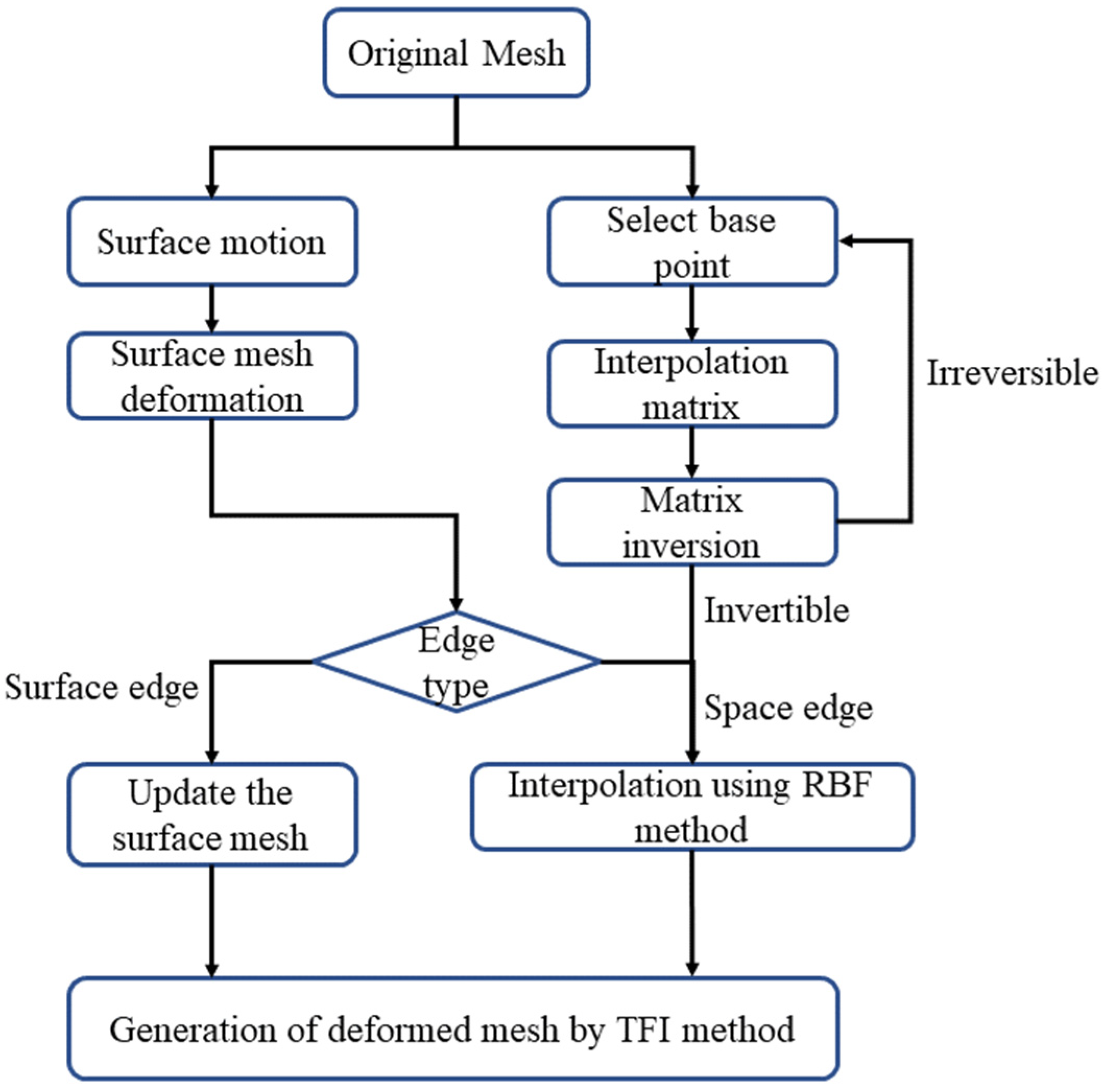
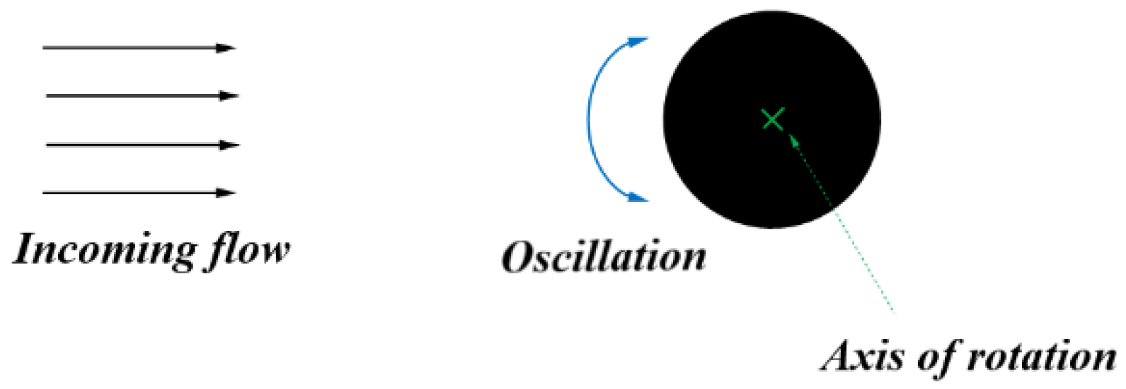
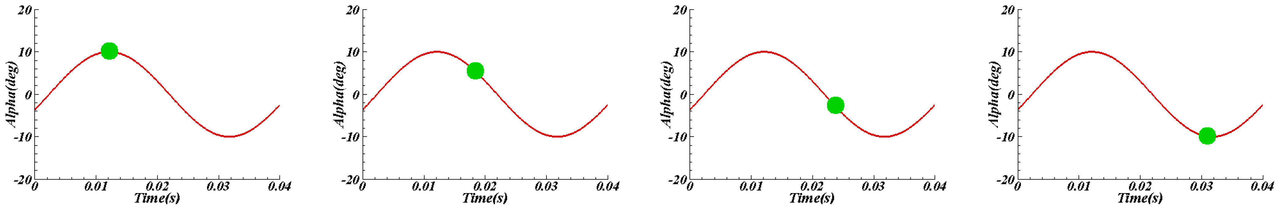
2.2. Computational Framework of Oscillatory Motion Noise

To study and analyze the aerodynamic and aeroacoustic performance of oscillating cylinders, a high-precision hybrid CFD/CAA prediction method was established, as shown in Figure 2. First, according to the characteristics of the CFD and CAA simulation, two sets of grids, named CFD grid and CAA grid, were prepared before solving the aerodynamic noise. Second, the time-averaged and turbulent variables on the CFD grid were obtained by solving the incompressible NS equations. Third, the time average flow information and turbulent information on the CFD grid were transferred to the CAA grid by using the self-developed “DataMap” code. The code is based on a k-Dimensional (KD) tree search algorithm and shapes function interpolation algorithm. Finally, the time average and turbulence information are provided to LPCEs to obtain the radiation sound field of the oscillating cylinder.

3. Reliability Test of Numerical Method

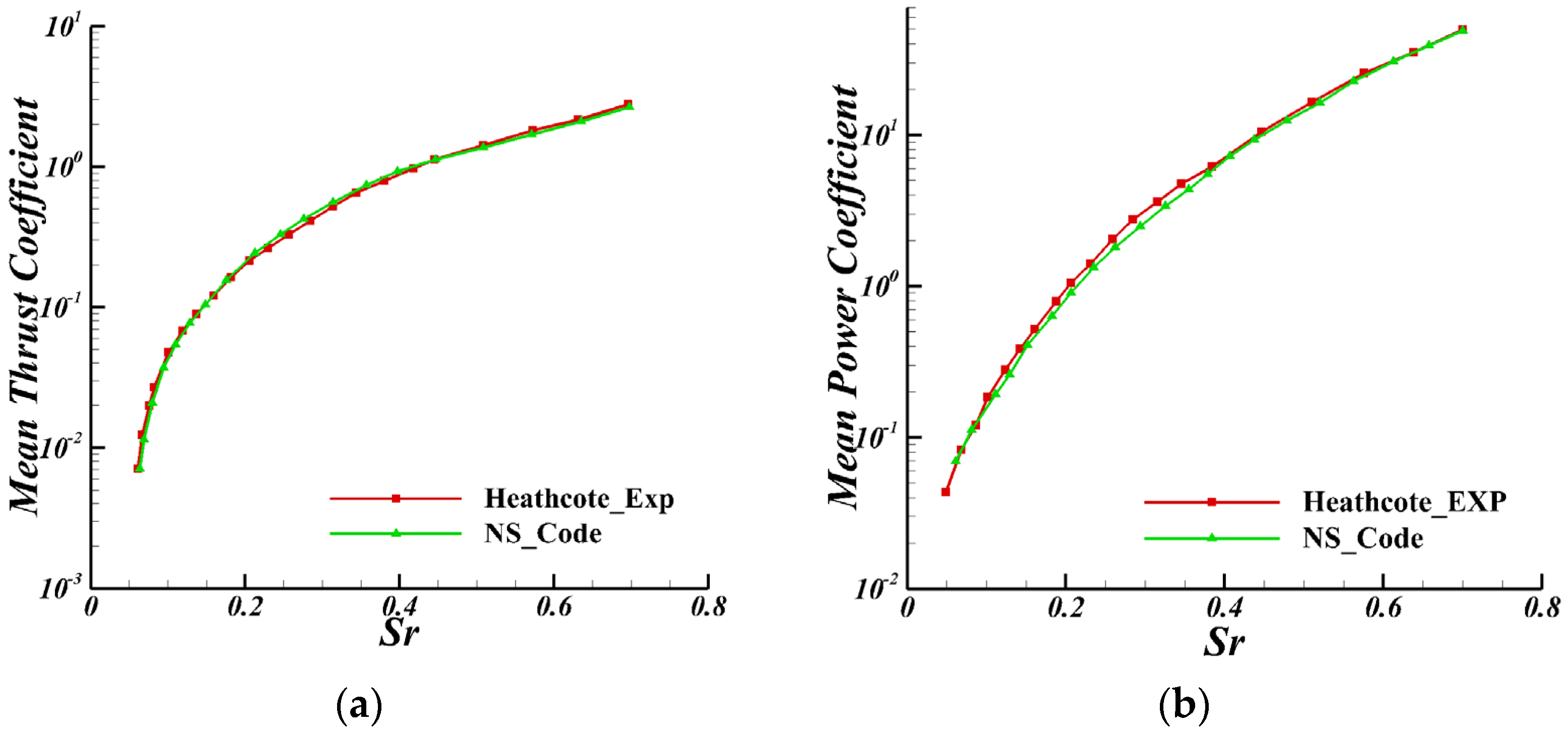
3.1. Aerodynamic Characteristics of an Oscillating Airfoil

In this section, the oscillating motion of the NACA0012 airfoil developed by Heathcote et al., was selected as the research object to validate the rationality of the CFD solution [26]. The oscillation amplitude of the airfoil was 0.175, the reduced frequency was in the range of 0.0 to 6.3, and the Reynolds number was 20,000. Figure 3 shows the comparison of the time-averaged thrust and power coefficient results by Heathcote et al. [26] with the CFD simulation results as a function of the Strouhal number S r . The flow was assumed to be fully laminar at the Reynolds number (Re = 20,000) for the CFD solver, and the results are shown in the figure with “NS_Code”. The expressions of the average tension coefficient and power coefficient in the figure are as follows:
C T = 1 T t t + T C D t d t C P = 1 T t t + T C L t y ˙ t + C M t θ ˙ t d t
where C D , C L and C M are the drag, lift, and moment coefficients, respectively. T is a period time of the force coefficient. y ˙ t and θ ˙ t are the heaving velocity and pitching velocity, respectively.
It is clear from the figure that the mean thrust coefficient and power coefficient calculated by the CFD solver were very consistent with the experimental results, although there was a small deviation near S r = 0.4 .

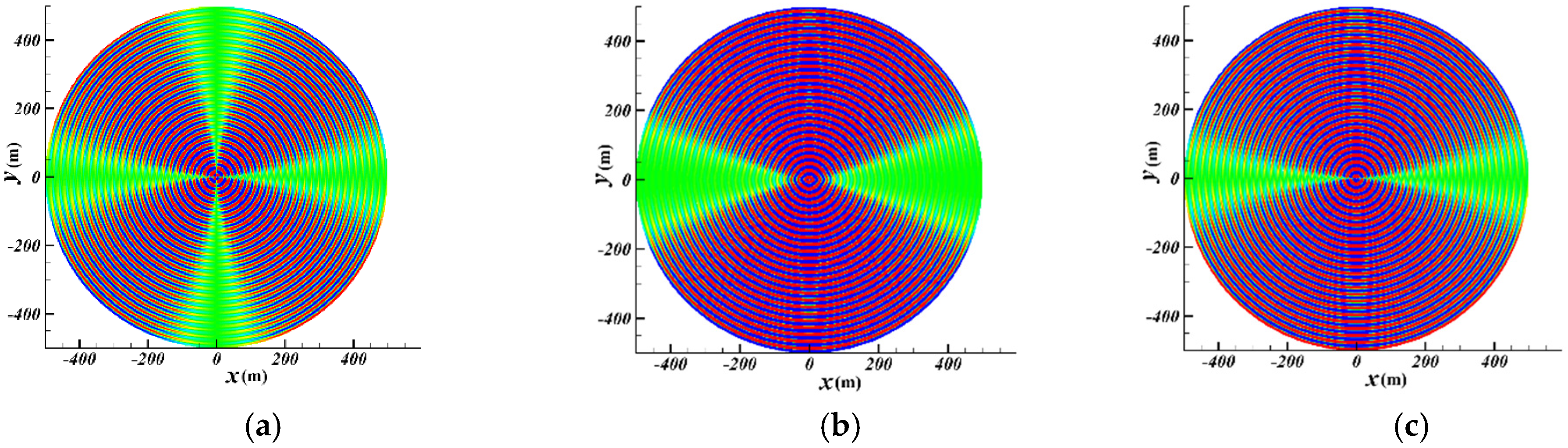
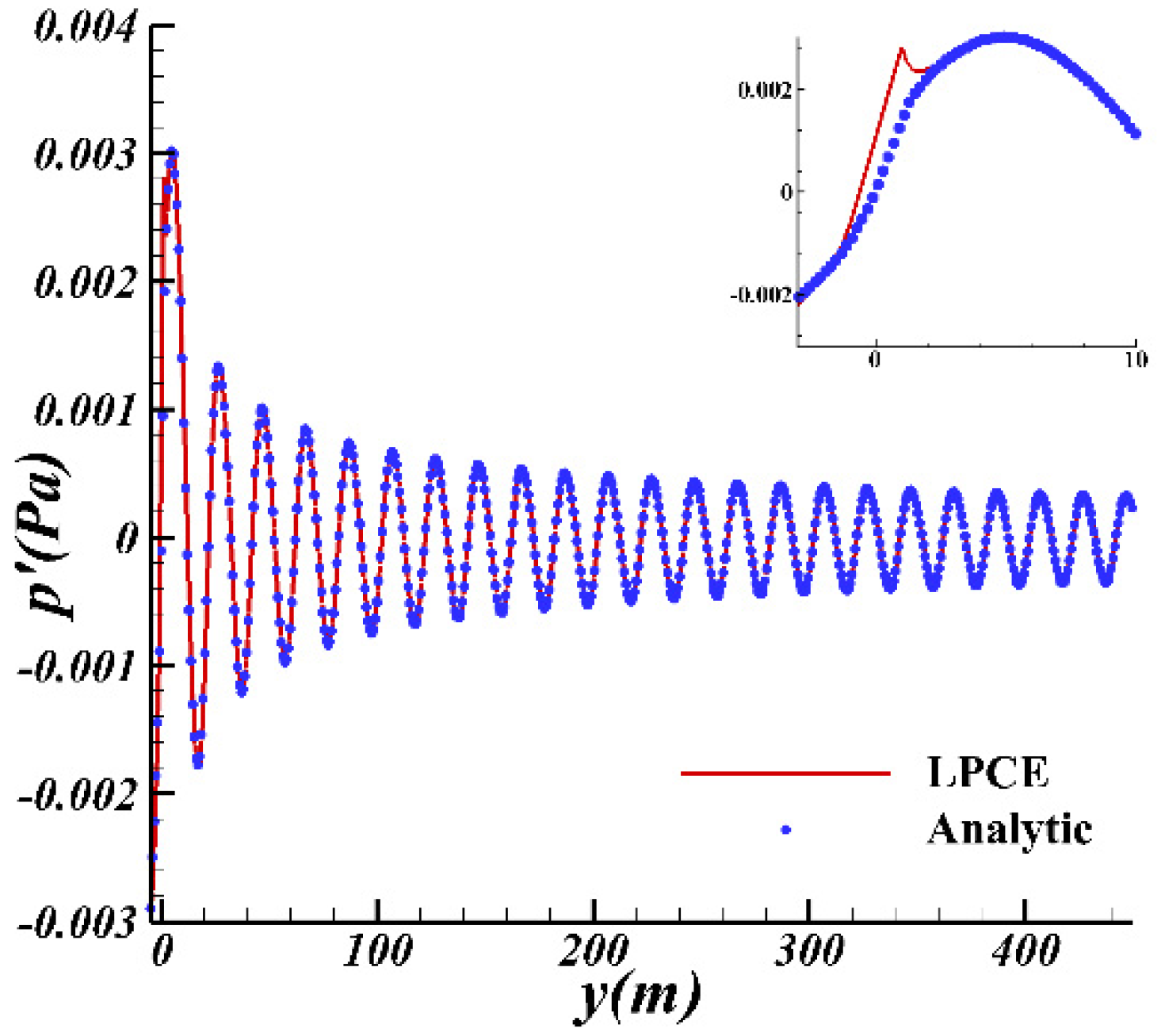
3.2. Dipole Sound Generation from an Oscillating Cylinder

To verify the effectiveness of the numerical method in the moving coordinate system, the dipole sound propagation from an oscillating cylinder was studied. As depicted in Figure 4, a cylinder located at the center of the computational domain oscillates with the defined periodic frequency. The radius of the whole computational domain was set to L = 500D, where D is the diameter of the cylinder. Here, the O-type grid was used, and 501 × 281 grid points were arranged in the radial and circumferential directions, respectively. The equation of motion of the cylinder is as follows:
h = d h sin 2 π K r t
where h is the amplitude of oscillation and was set to 0.01 and K r is the oscillation frequency, which was set to 0.05.
A quiescent air was used as an initial condition and the maximum translational velocity of an oscillating cylinder was 0.03. The Reynolds based on the cylinder diameter and maximum translational velocity was set to 1780. The INSE/LPCE hybrid method was used for sound field prediction.
The spatial distribution of flow pulsating velocity, normal pulsating velocity, and pulsating pressure is shown in Figure 5. Among them, the same scale was used for the distribution of flow pulsating velocity and normal pulsating velocity. The intensity of normal pulsating velocity was higher than that of the flow pulsating velocity. The distribution of the fluctuating pressure presents dipole characteristics. Figure 6 shows the comparison between the numerical prediction and the analytical solution of the pulsating pressure on the x = 0 line. The analytical solution (for detailed derivation, see [27]) is as follows
p x , t = π 3 K r 2 ρ ¯ D 2 U ¯ 2 c ¯ cos φ J 1 2 π K r x c ¯ + i N 1 2 π K r x c ¯ e 2 π i K r t
where K r is the oscillation frequency; c ¯ is the speed of sound; and D is the diameter of the cylinder. U ¯ = 2 π K r × d h is the maximum velocity at the cylinder surface. φ is defined as an angle measured from the plane of vibration. J 1 denotes the Bessel function first kind order one, and Neuman function N 1 is a Bessel function second kind.
The INSE/LPCE result is in excellent agreement with the analytical solution except at y close to 0, in which any viscous effects were not taken into account.

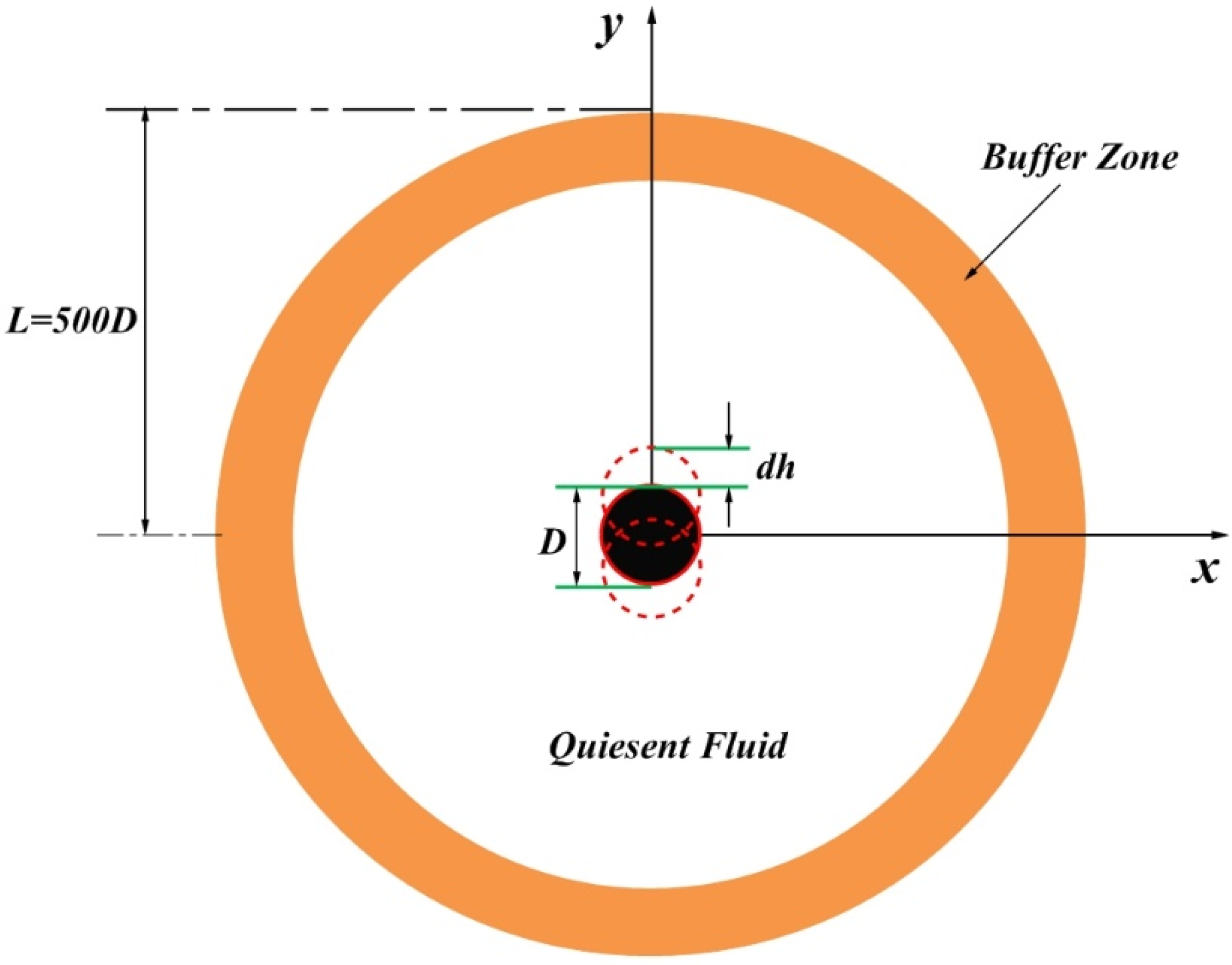
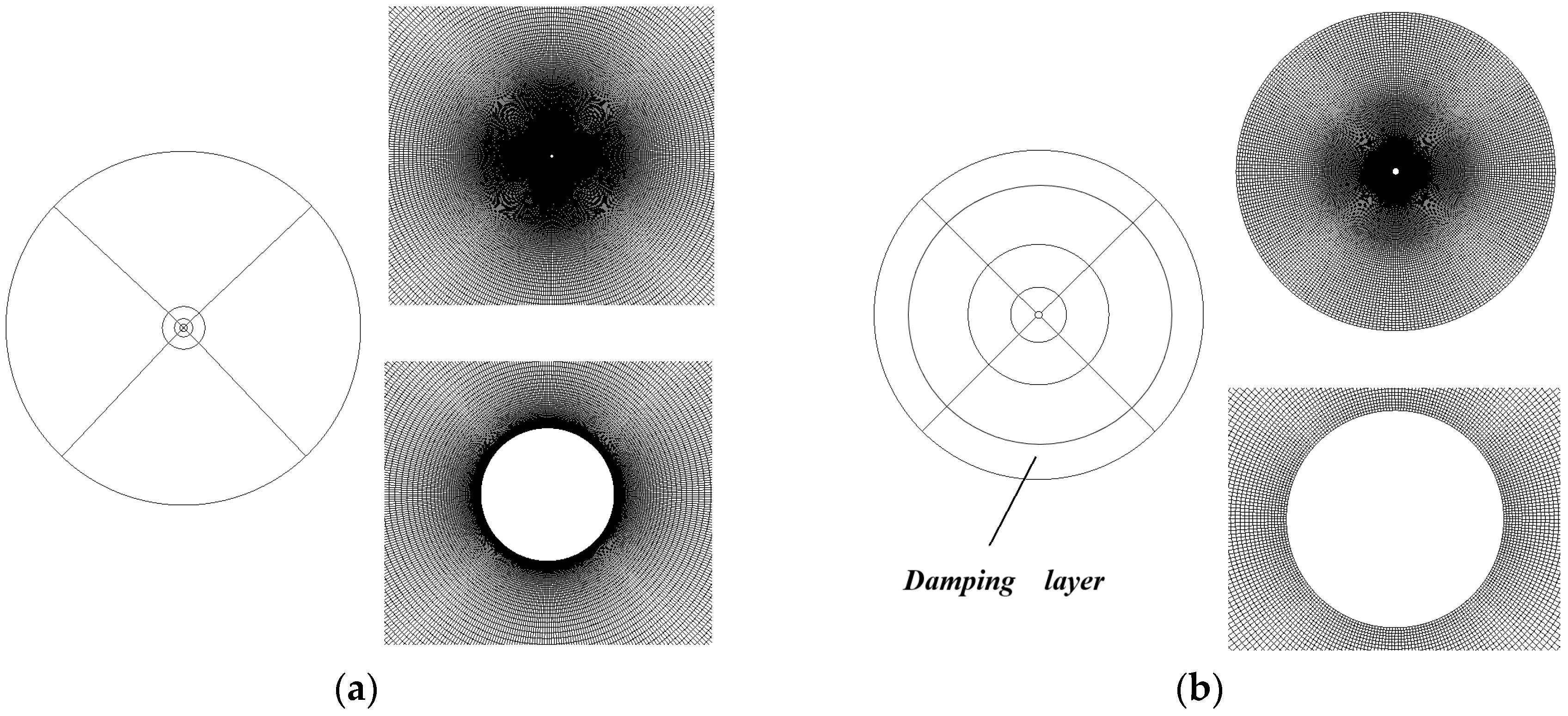
4. Calculation Settings

In this section, we studied the aerodynamic and aeroacoustic characteristics of a single cylinder with a diameter of 2 m. The schematic diagram of the oscillating cylinder is shown in Figure 7. The axis of rotation of a cylinder is at the center of the cylinder. The calculation conditions were as follows: the incoming Mach number was 0.05, Reynolds number per unit length based on cylinder diameter was 1.0 × 10⁵. The cylinder oscillatory motion can be expressed as:
θ   =   θ 0 + θ ˜ max   π 180 sin 2 π K r t L r e f    
where θ ˜ max denotes the oscillation amplitude; θ 0 is the base angle of attack. The units of variables θ ˜ max and θ 0 are degrees. K r is the oscillation frequency; t is the oscillation time; L r e f is the reference length, which is equal to 1.
To examine the effects of both oscillation frequency and amplitude on the aerodynamic and aeroacoustic characteristics of an oscillating cylinder, four groups of motion parameters are given, as shown in Table 1.
Before determining the CFD grid topology and the number of grid points, we divided five CFD grids of different sizes, and the grid sizes were about 50,000, 100,000, 200,000, 300,000, and 400,000. Here, we used the motion parameters in Case1 as the calculation conditions to carry out the CFD grid independence analysis. For the CFD flow field of an oscillating cylinder, the calculation strategy is as follows. First, the Reynolds average INS equations were used to calculate the steady flow field, which was regarded as the initial flow field. Then, the transient flow field of the cylinder oscillation was solved by the CFD method based on dynamic grid technology, in which the dimensionless time step was 0.03. Table 2 shows the average value of the drag coefficient and the disturbance amplitude of the drag coefficient under grids of different scales, which are defined as follows:
C l t = F y 0.5 × ρ inf × V inf 2 × A C d t = F x 0.5 × ρ inf × V inf 2 × A C d a v e = 1 T t t + T C d t d t C l a v e = 1 T t t + T C l t d t C d A m p = max C d t min C d t ,    t t , t + T C l A m p = max C l t min C l t ,    t t , t + T
where F y is the lift; F x is the drag; ρ inf is the reference density at infinity; V inf is the velocity of the incoming flow at infinity; and A is the reference area, where the value is selected as 1 m 2 .
From Table 2, we can see that when the grid size was above 300,000, the drag coefficient tended to converge. The topology of the CFD and CAA computation grids finally used in the paper is shown in Figure 8, in which the CFD grid comprised 308,000 nodes and the CAA grid was 104,000 nodes. Due to the difference in the physical field between CFD and CAA, the grid distribution also showed an obvious difference. For the CFD grid, the focus was more on the grid density near the wall and the separation zone. For the CAA grid, orthogonality and uniformity are more important. It should be noted that the distribution of orthogonality and the slenderness ratio of the CAA grid meets the requirement of grid points for one wavelength.

5. Results and Discussion

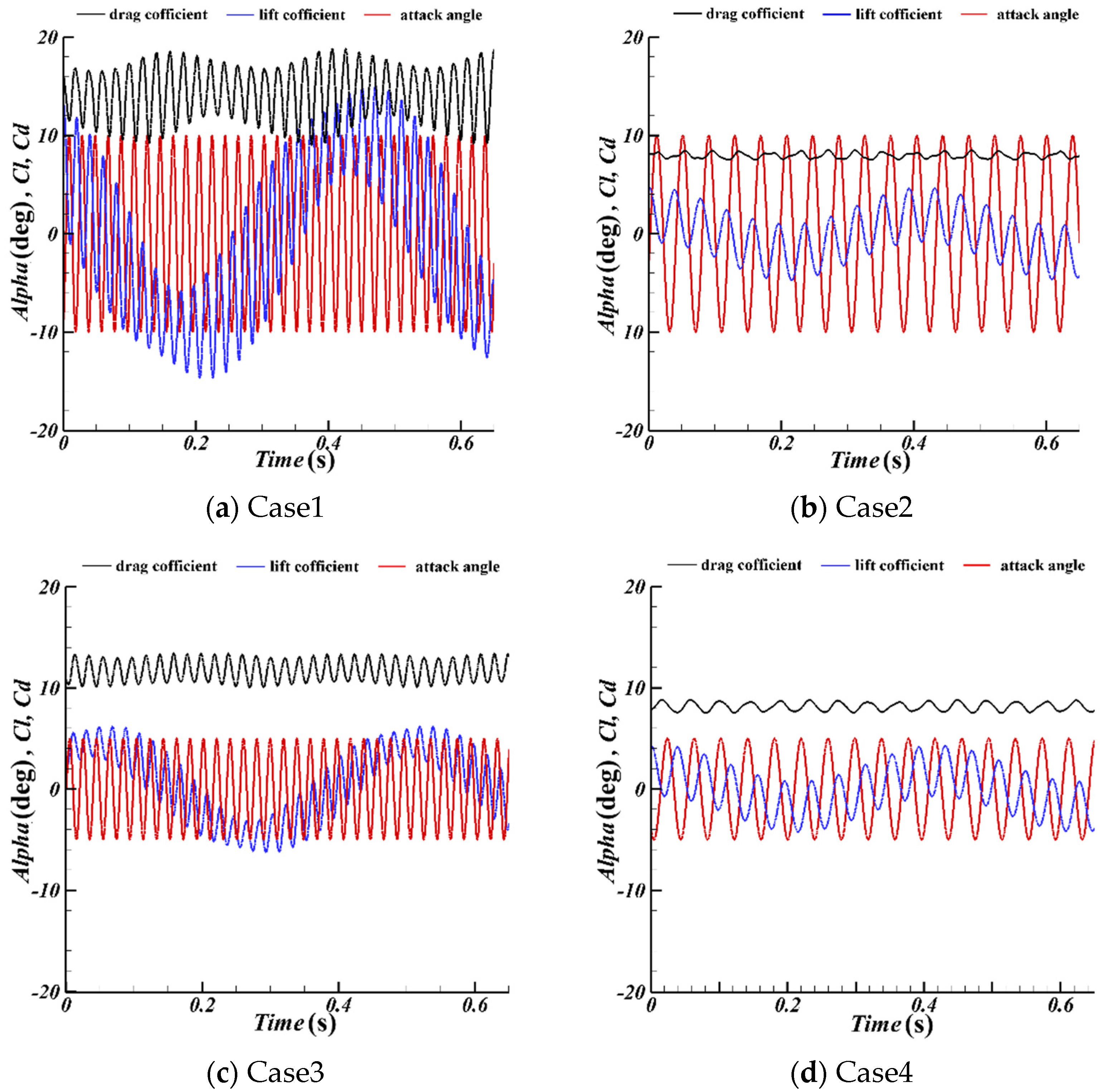
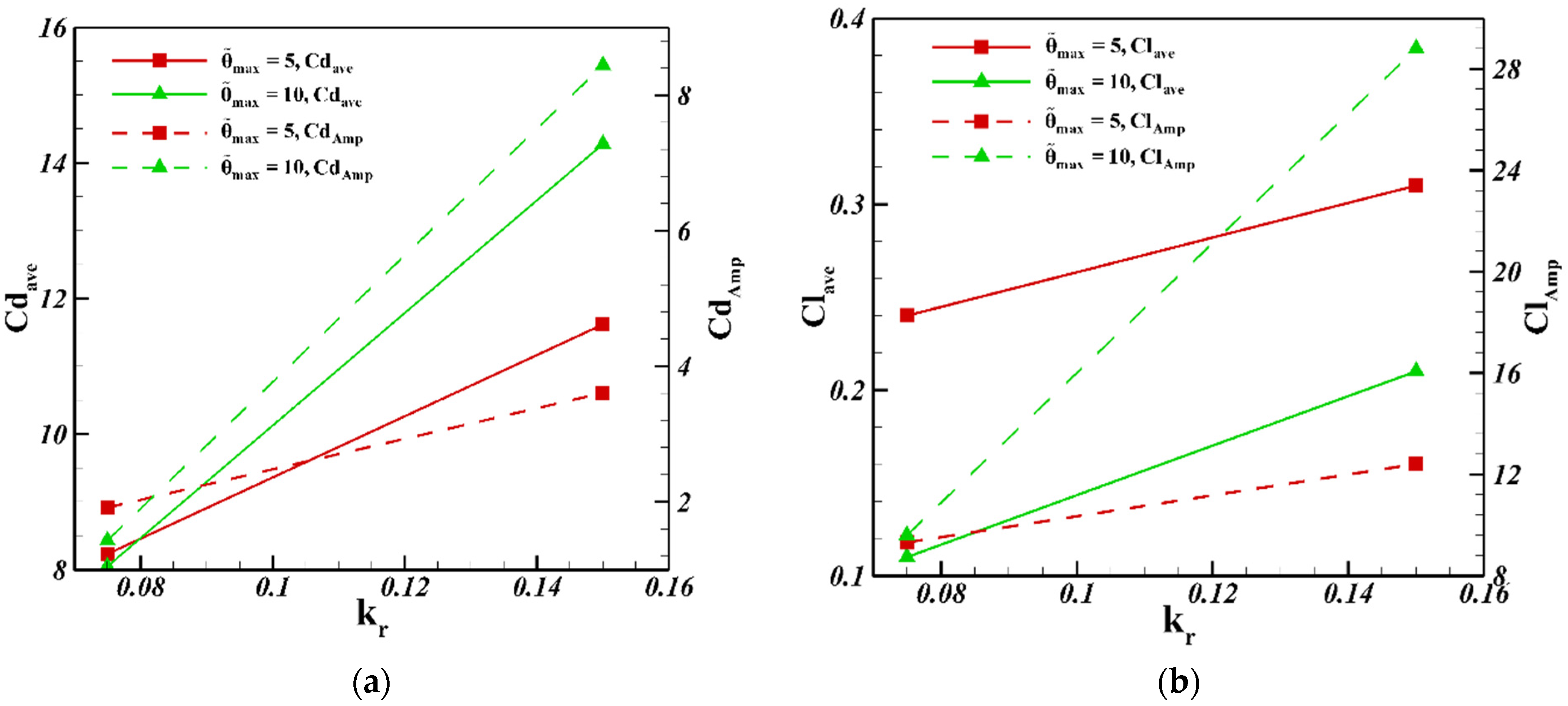
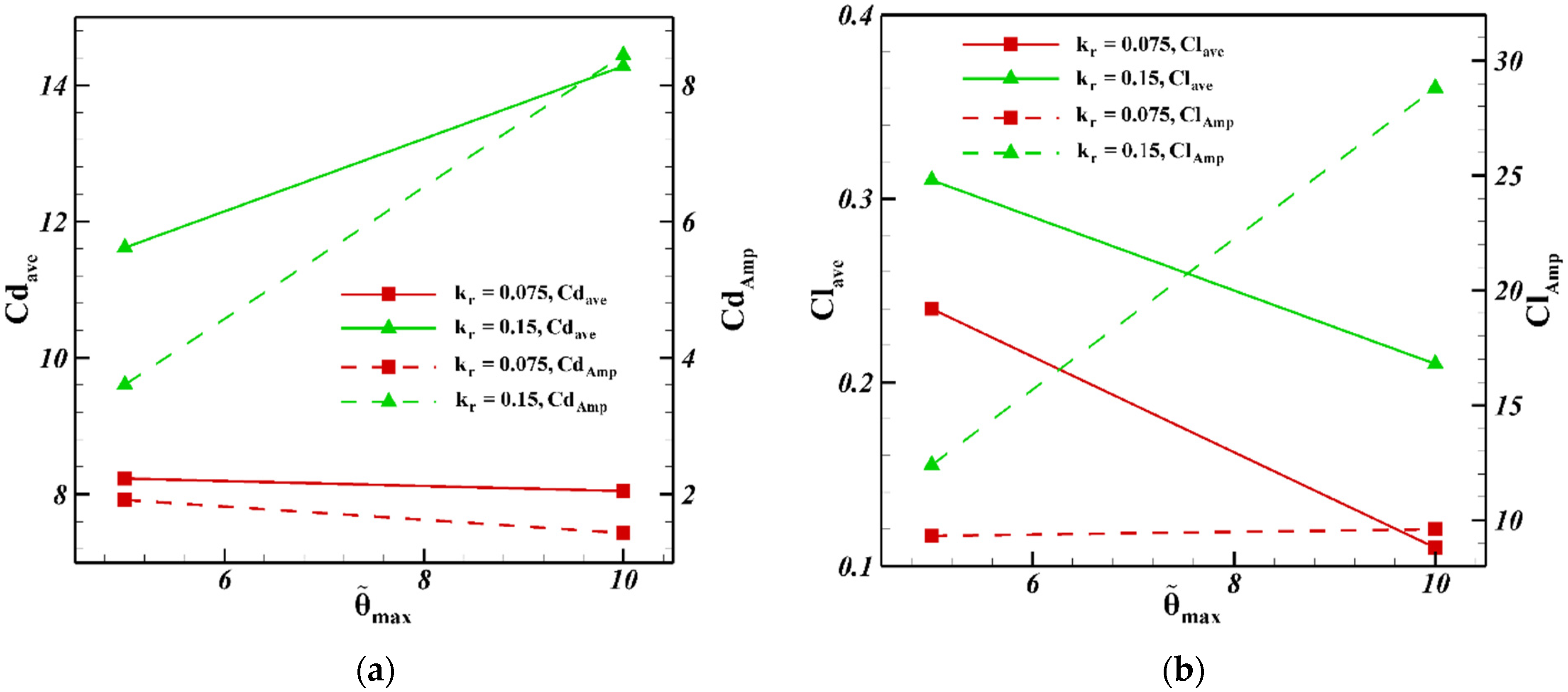
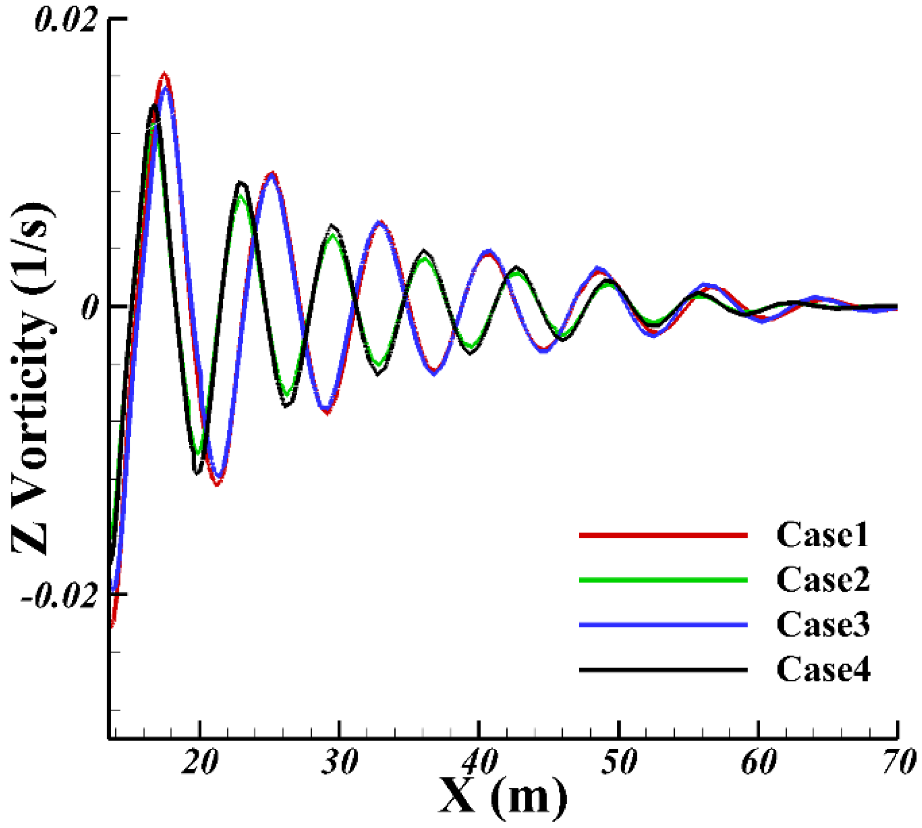
5.1. Aerodynamic Characteristics

Figure 9 shows the variation curves of the angle of attack, lift coefficient, and drag coefficient with time for different configurations after convergence of the flow field calculation. Several phenomena can be seen in Figure 9. The curves of the lift coefficient and drag coefficient showed that there were two obvious periods. The small period corresponded to the rotation frequency of the cylinder, the other period was independent of the rotation frequency, and the periods of each configuration were the same. When the rotation frequency was the same, the larger the rotation amplitude, the larger the variation range of the lift and drag coefficients, and the larger the average value of the drag coefficient. When the rotation amplitude was the same, the greater the rotation frequency, the greater the variation range of the lift drag coefficient, and the greater the average value of the drag coefficient. Compared with Case2 and Case3, the effect of rotation frequency on lift and drag coefficient was greater than that of the rotation amplitude.
Table 3 gives the specific value of the change in the lift-drag coefficient of the oscillating cylinder under each motion state. The values in parentheses in Table 3 represent the percentages of the lift-drag coefficients of each motion state (Case1, Case2, Case3, and Case4) to the simulation results of the Case1 state. The meanings of C d a v e , C d A m p , C l a v e , and C l A m p in the table can be found in Equation 14. We plotted the data in Table 3 as Figure 10 and Figure 11. Figure 10 is the change curve of the lift resistance coefficient ( C d a v e , C d a v e , C d A m p , C l a v e , and C l A m p ) with the oscillation frequency under the condition of constant amplitude oscillation, and Figure 11 is the change curve of the lift resistance coefficient with the oscillation amplitude under the condition of constant frequency oscillation. By comparing and analyzing the data in Table 3 and the curves in Figure 10 and Figure 11, it can be found that when the oscillation amplitude was the same, the changes in the C d a v e , C d A m p , C l a v e , and C l A m p values increased with the increase in the oscillation frequency. This phenomenon was more obvious in the large oscillation amplitude. For the same small oscillation frequency ( k r = 0.075 ), the oscillation amplitude had little effect on the C d a v e , C d A m p , and C l A m p values. However, for the same large oscillation frequency ( k r = 0.15 ), the C d a v e , C d A m p , and C l A m p values will increase with the increase in the oscillation amplitude.
To explain the variation trends of the lift and drag coefficient in Figure 10 and Figure 11, the variations in the z-vorticity and pressure in different periods are described in Figure 12 and Figure 13, respectively. Figure 12 shows the Z vorticity snapshots of the four configurations in the period time T = 0.425. Comparing the Z vorticity of Case1, Case2, Case3, and Case4, we can reach some conclusions. First, it can be preliminarily judged that the large period of the lift and drag coefficients are related to the frequency of the shedding vortex. To further illustrate this result, Figure 13 presents the Z vorticity distribution curves of the four configurations simultaneously at the y = 0 station. For ease of comparison, the starting points of the four curves were adjusted to the same location. It can be seen from the figure that the vorticity frequencies of Case1 and Case3, Case2 and Case4 were the same. Second, compared with Case1 and Case2, Case3 and Case4, the distribution range of the Z vorticity was larger when the rotation frequency was higher at the same rotation amplitude. In addition, when the frequency was higher, the length of the wake in the leeward region was shorter. Third, compared with Case1 and Case3, Case2 and Case4, the distribution range of the Z vorticity was larger with the increase in the rotation amplitude at the same rotation frequency.
Taking Case2 as an example, Figure 14 shows the pressure snapshots in a rotation cycle. From the comparative analysis of the figure, we can draw the following conclusions: (1) Due to the periodic rotation of the cylinder, the flow variables interact to form positive and negative intersecting pressure waves; and (2) with the rotation of the cylinder, the pressure disturbance also changes with the rotation.

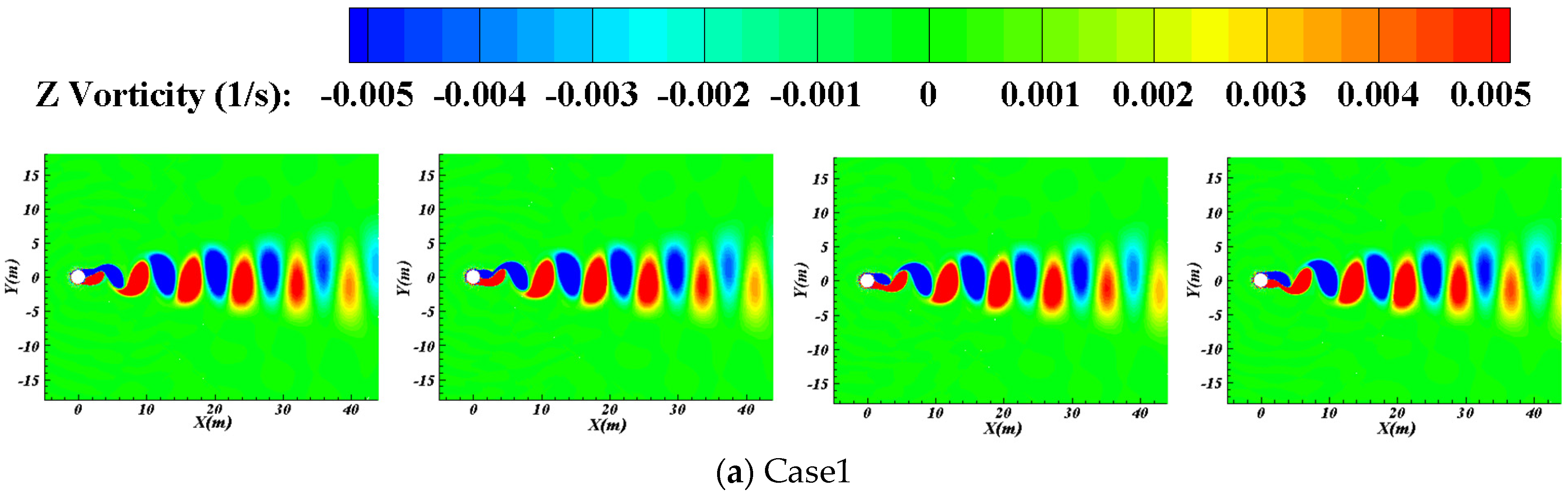
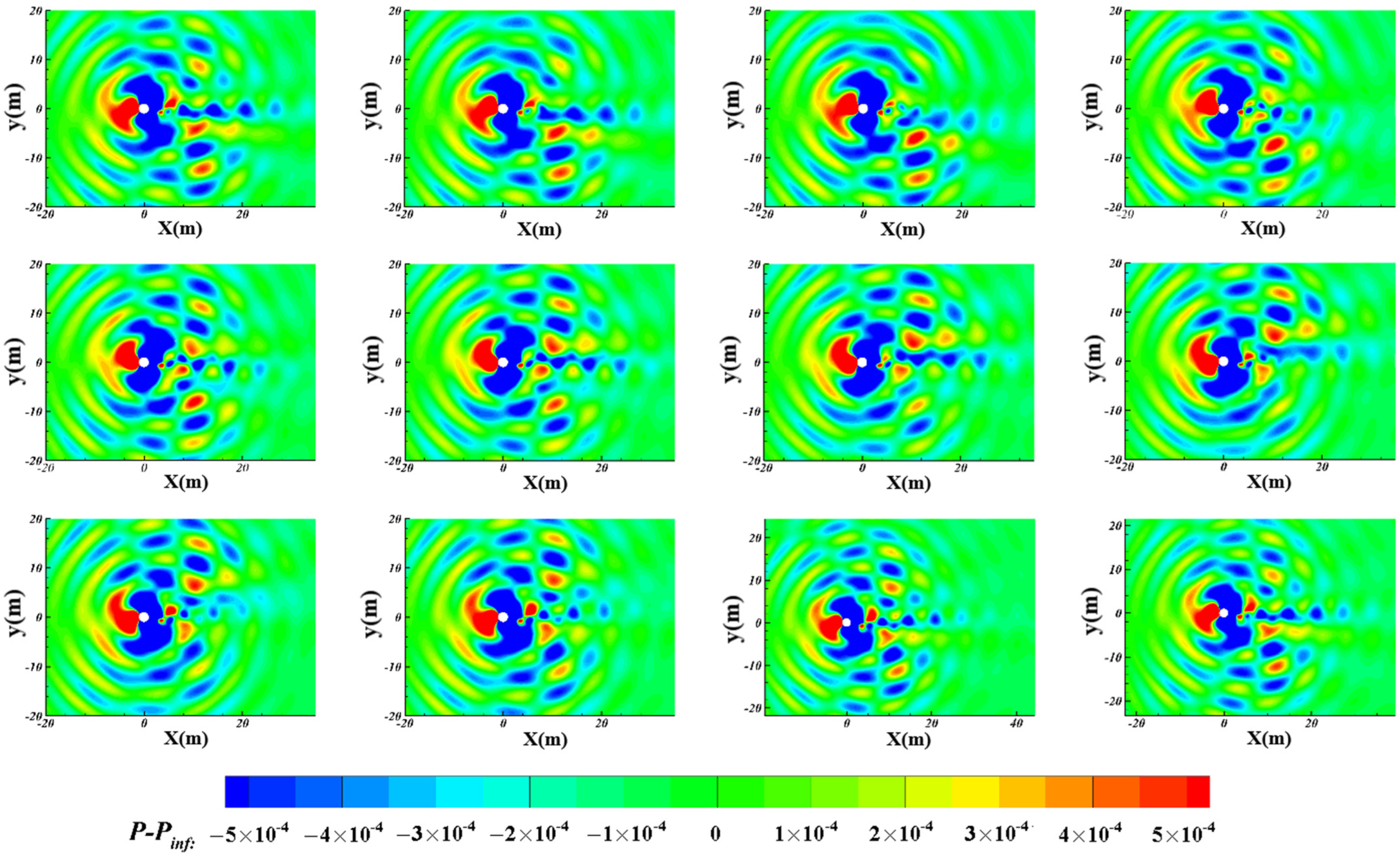
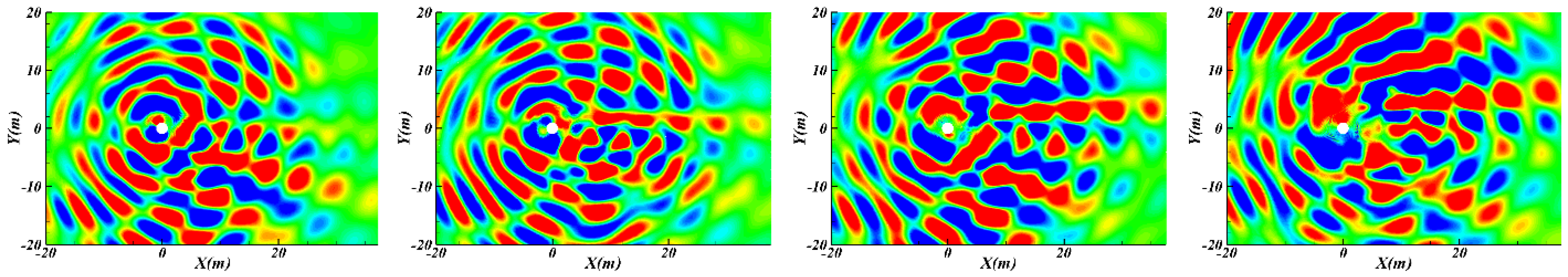
5.2. Aeroacoustic Characteristics

Figure 15 shows the sound pressure propagation of Case2 over one rotation cycle. It can be seen that the rotation angle of the cylinder changed from positive ten degrees to negative ten degrees, and the sound pressure in the space changed counterclockwise, and vice versa. This is a phenomenon caused by the superposition of the flow rotation effect and the sound wave propagating around. Figure 16 shows the instantaneous sound field when the sound wave reaches the far field boundary. It can be seen that under the condition of low-speed incoming flow, the larger the rotational frequency or amplitude of the cylinder, the stronger the noise intensity induced by the turbulent flow. For the current calculation conditions, the maximum intensity of the sound wave was located near the normal of the cylinder, and there was obvious sound wave interference at other positions. For Case1 and Case2, the forward noise intensity was significantly greater than the backward noise intensity.
To further analyze the frequency characteristics of the sound waves, the dynamic mode decomposition (DMD) method (the code comes from http://www.ece.umn.edu/users/mihailo/software, accessed on 8 September 2021.) was used to analyze the contribution of different frequencies of sound waves for Case2. The snapshot matrix was analyzed by the DMD method [28]. According to the development of modal coefficients with time, the contribution of different modes to the acoustic field is sorted, and the first several main modes are extracted for analysis. The relationship between the amplitude and frequency of each mode is shown in Figure 17. It can be seen that the modes captured were sorted according to the amplitude, and the main energy of the sound field was concentrated on the first and second modes. The main modal eigenvalues are shown in Figure 18. It can be seen that the selected modes were close to the unit circle, and the first several modes fell on the unit circle. This means that these modes did not change with the sound field, and their growth/decay rate was close to 0. Corresponding to Figure 17, we extracted the cloud images with frequencies of 25, 50, 75, 100, and 125 Hz, as shown in Figure 19. The distribution of each frequency was quite different in the whole computational domain, which indicates that these modes can reflect the periodic change of sound waves with time.
Next, 36 monitoring points were arranged in the space to analyze the characteristics of the sound pressure level (SPL) spectral and the directivity of the overall SPL. The distance between the monitoring points and the rotating axis of the cylinder was 50 m, as shown in Figure 20. The overall sound pressure level (OASPL) curve is shown in Figure 21. This shows that the OASPL values of the four configurations were symmetrically distributed along the y = 0 . For Case4, there were obvious low OASPL values near 0, 100, 180, and 260 degrees, and high OASPL values near 70 and 290 degrees. Similar to Case4, Case3 had low OASPL values at 100 and 260 degrees, and high OASPL values at 70 and 290 degrees. Unlike Case4, Case3 had no obvious low OASPL values in the 0~180 angle regions. Compared with Case4, the OASPL intensity distribution of Case1 and Case2 were more uniform. When one motion parameter in rotation amplitude or rotation frequency was constant, the difference of OASPL value was more obvious with the increase in the other parameter.
Figure 22 shows the comparison of the sound pressure level spectrum curves of the monitoring points P1, P2, P3, and P4, where P1 is the harmonic frequencies of Case2 and Case4 states. The Case1 and Case3 states were similar, corresponding to the change frequency in the lift and drag coefficient curves. The first harmonic frequency of the Case2 and Case4 states was 22 Hz and the second harmonic frequency was 48 Hz; the first harmonic frequency of the Case1 and Case3 states was 50 Hz and the second harmonic frequency was 100 Hz. The harmonic characteristics of the other monitoring points (P2, P3, P4) were similar to P1 for all states. To sum up the above description, that is, the frequency corresponding to the high sound pressure level corresponds to the multiple of the rotation frequency of the cylinder. In addition, for the four monitoring points, the maximum sound pressure level under the calculation conditions of Case2 and Case4 ( K r = 0.075) states was mainly concentrated in the vicinity of the second harmonic frequency. However, for the Case1 and Case3 ( K r = 0.15) states, the concentrated harmonic frequencies of the maximum sound pressure level were uncertain, hovering between the first two harmonic frequencies. This may be due to the mutual interference of the oscillation frequency with the natural vortex shedding frequency of the cylinder, the effect of changing flow patterns, and rotational oscillations.

6. Conclusions

A high accuracy numerical method based on INSE/LPCE was developed to calculate the unsteady aerodynamic and acoustic characteristics of a rotating oscillating cylinder. Four groups of different rotation frequencies and amplitudes were studied including the lift drag coefficient, noise directivity, and spectrum characteristics. The conclusions obtained in this paper were as follows.
  • Among the several groups of motion parameters studied, when the oscillation amplitude is the same, the variation amplitude of the lift-drag coefficient will increase with the increase in the oscillation frequency. Moreover, this phenomenon is more pronounced when the oscillation amplitude is larger. For the same small oscillation frequency ( k r = 0.075 ), the oscillation amplitude has little effect on the variation in the lift-drag coefficient. However, for the same large oscillation frequency ( k r = 0.15 ), the variation amplitude of the lift-drag coefficient will increase with the increase in the oscillation amplitude.
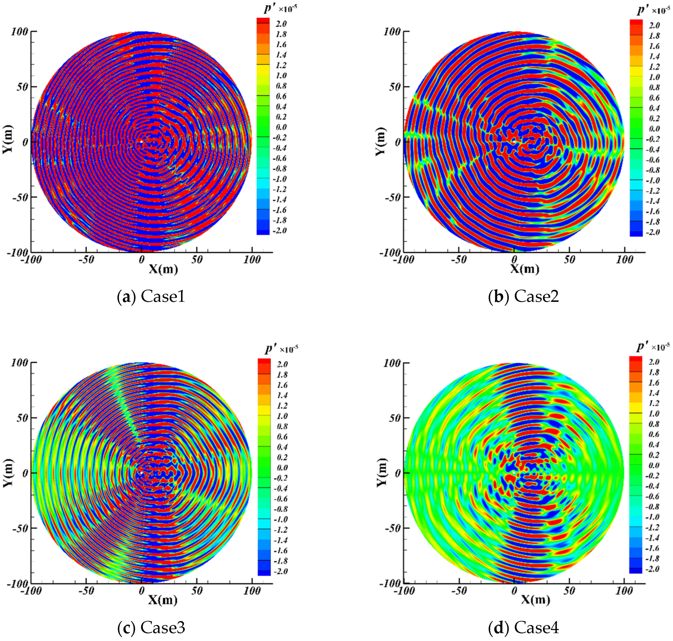
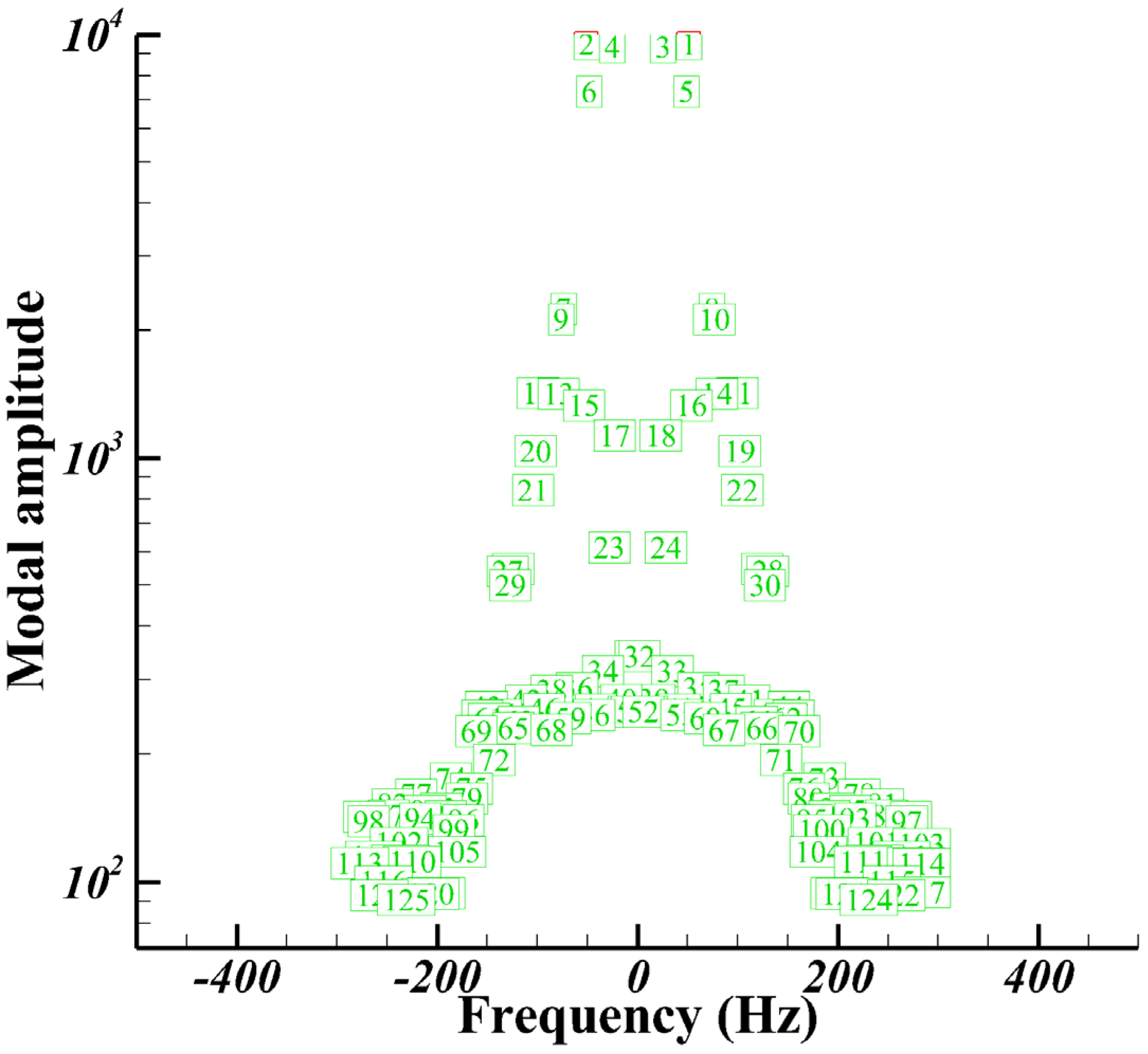
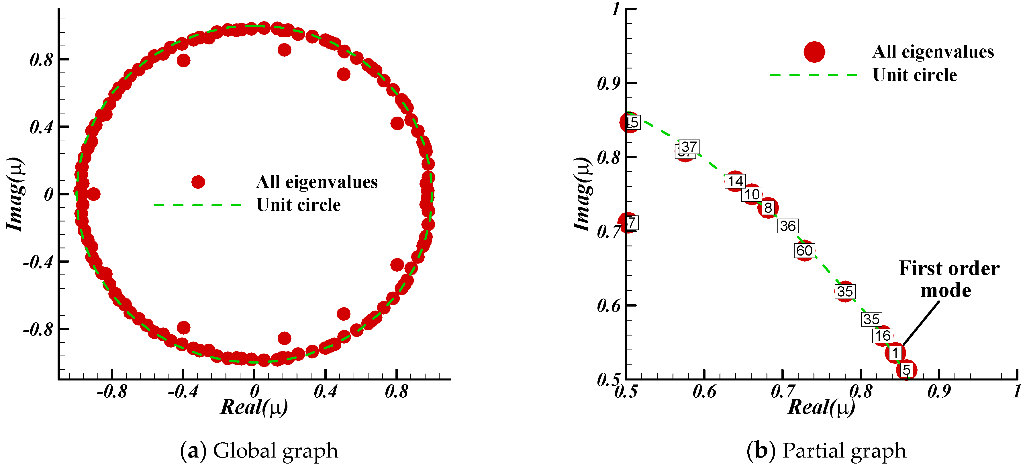
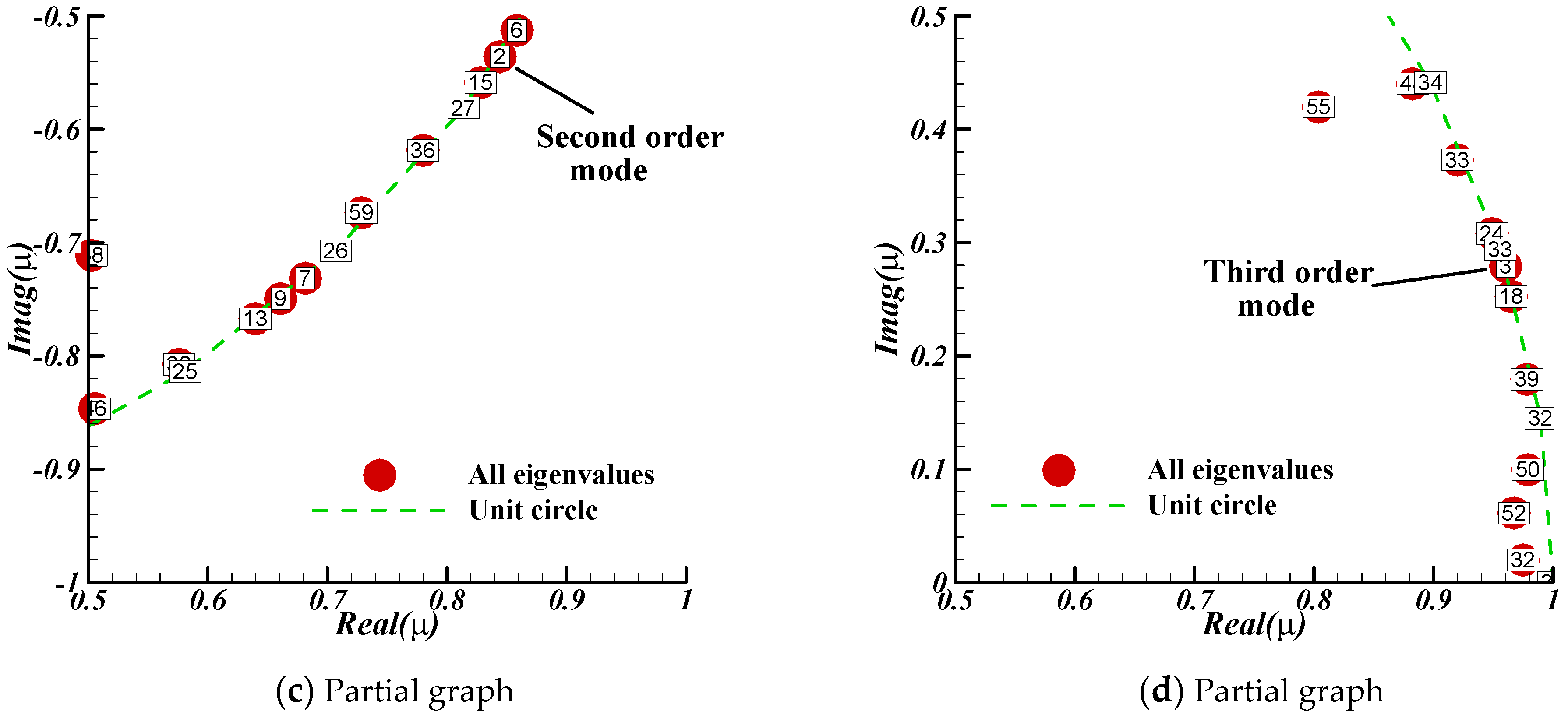
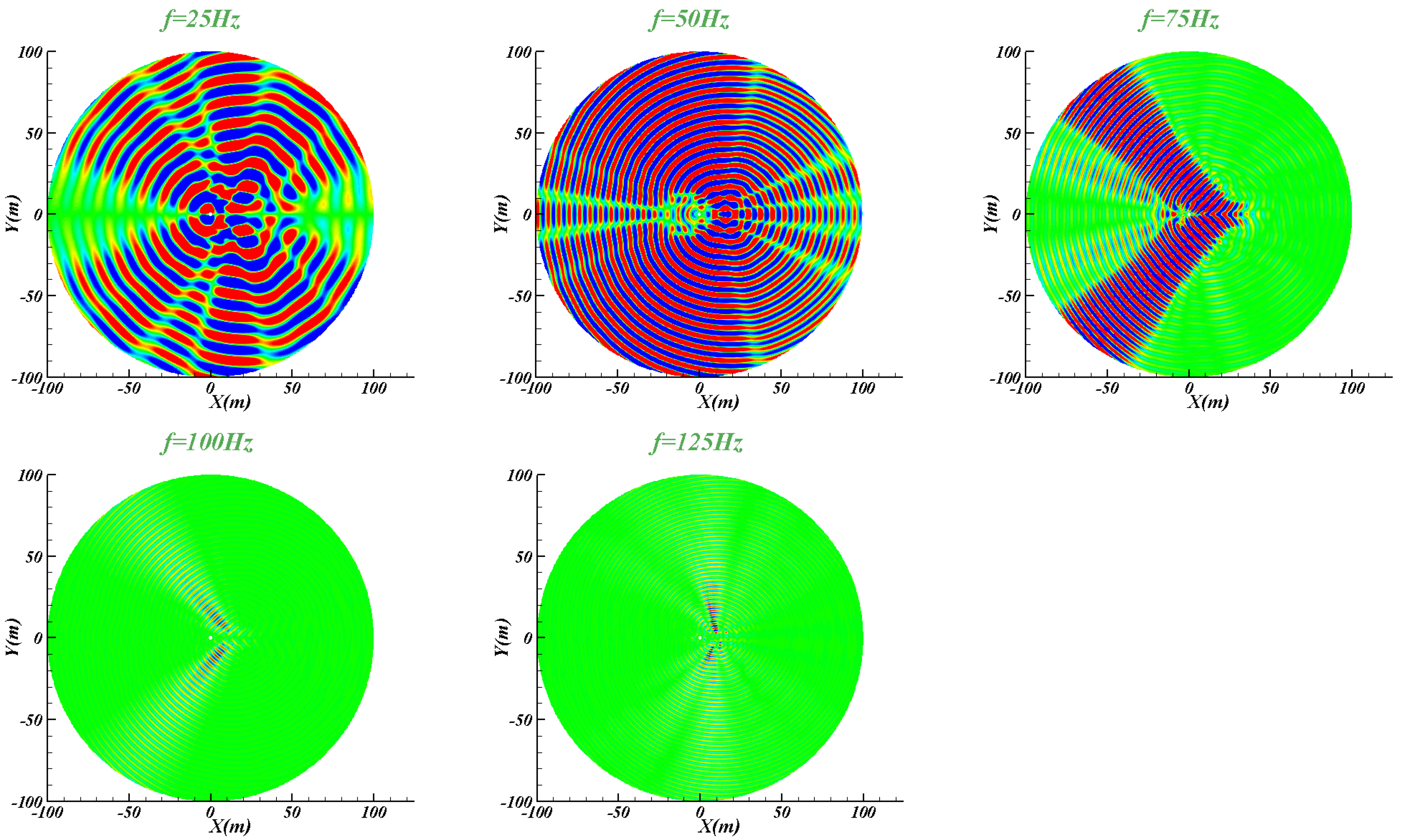
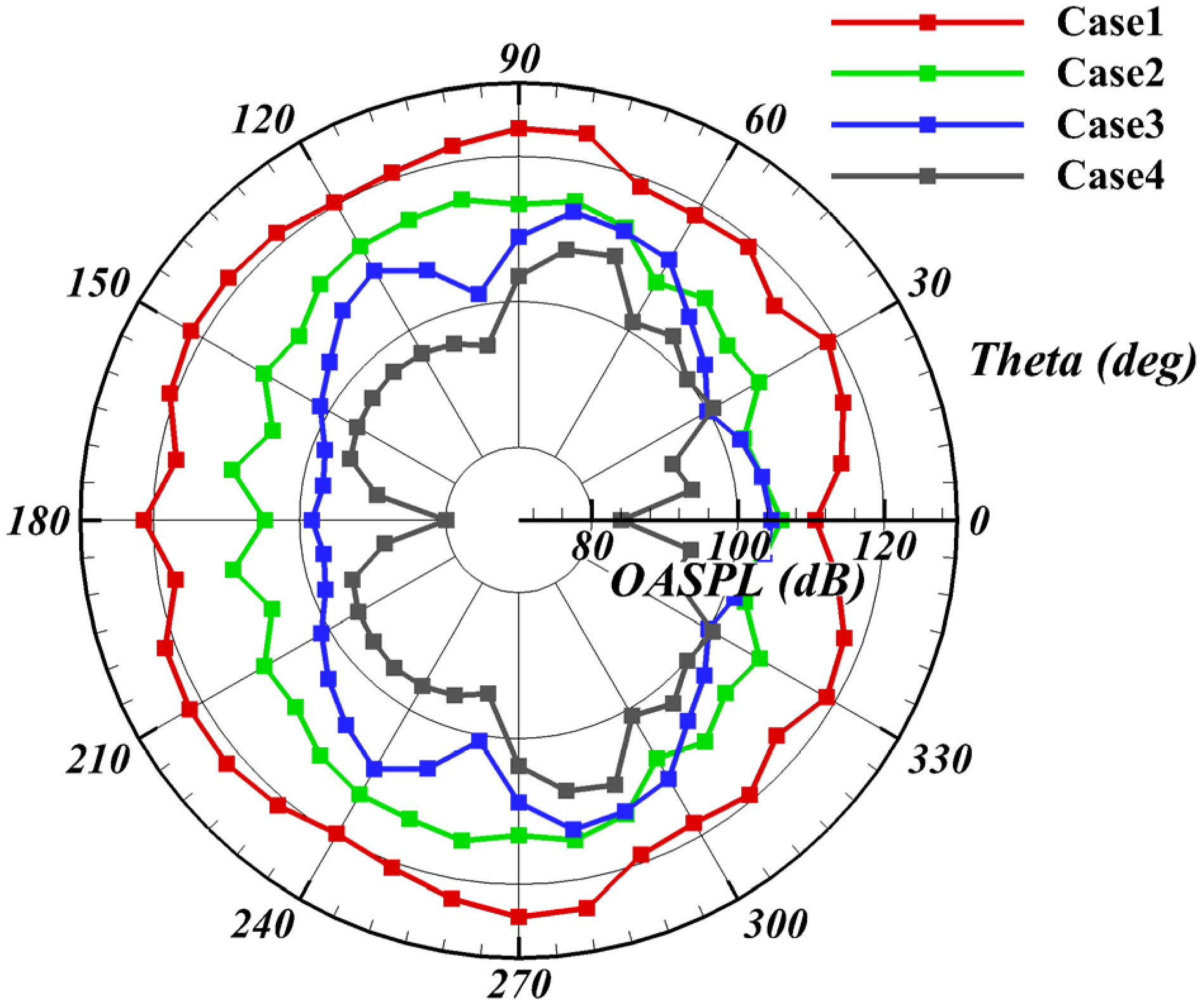
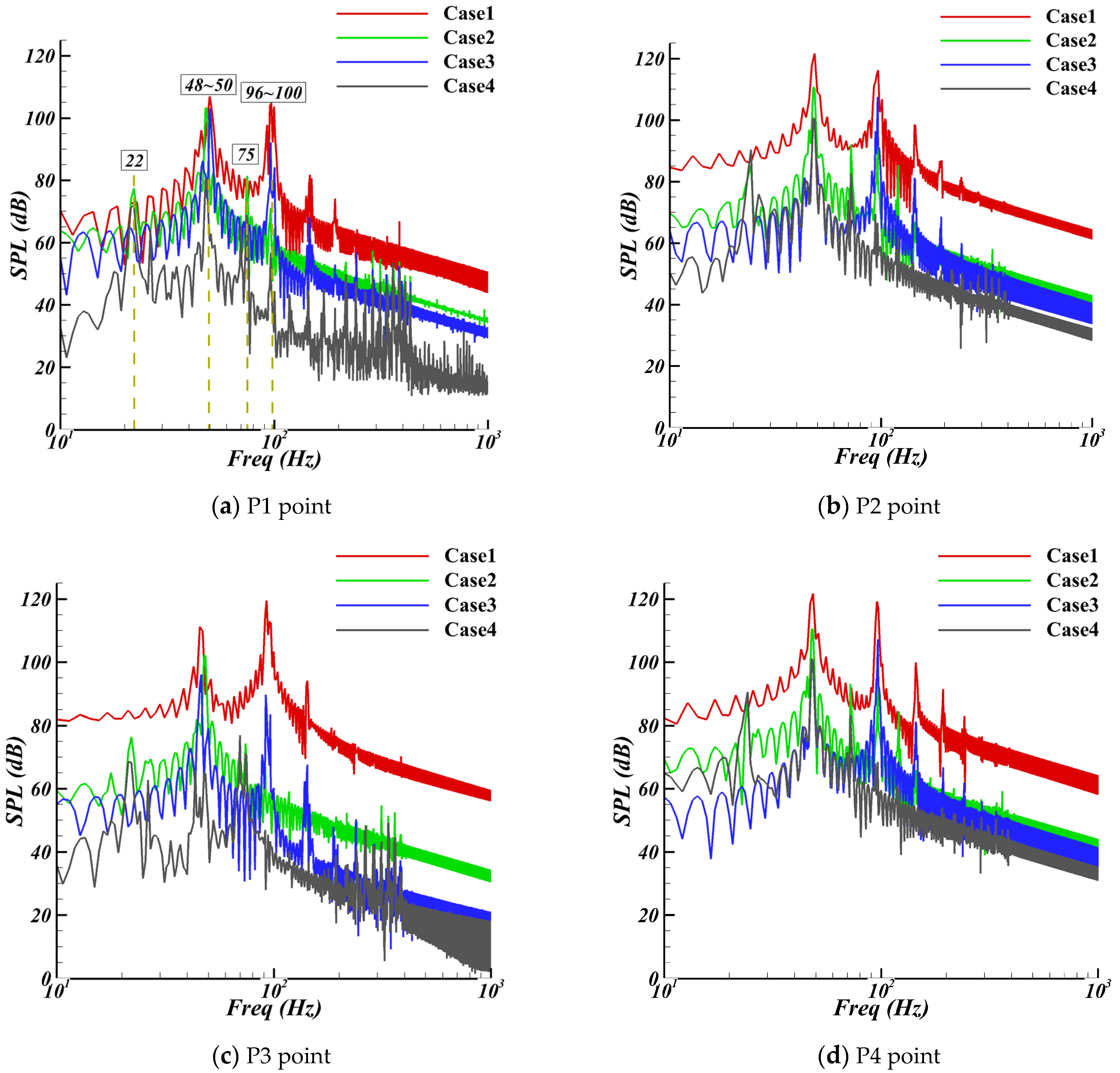
  • Under low-velocity incoming flow conditions, the greater the rotational frequency or amplitude of the cylinder, the greater the noise intensity caused by the turbulent flow. For the current calculation conditions, the maximum intensity of the sound wave was located near the normal of the cylinder, and there was obvious sound wave interference at other positions. For the state of the large rotation amplitude, the intensity of the front-pass noise was significantly greater than that of the back-pass noise. In addition, after the DMD method analysis, it can be concluded that the main energy of the sound field was concentrated at the first and second-order narrowband frequencies.
  • There are many flaws in this paper. For example, if the oscillation amplitude and oscillation frequency change sufficiently, locking may appear, which has the potential to greatly affect the behavior of the cylinder in terms of aerodynamics and aeroacoustics. This will be the focus of our next research work.

Author Contributions

Conceptualization, P.Y. and J.X.; methodology, P.Y.; software, H.X.; validation, P.Y. and J.X.; formal analysis, J.X.; investigation, J.X.; resources, H.X.; data curation, J.X.; writing—original draft preparation, P.Y.; writing—review and editing, P.Y.; visualization, P.Y.; supervision, J.X.; project administration, J.B.; funding acquisition, J.B. All authors have read and agreed to the published version of the manuscript.

Funding

This work was supported by grants from the National Natural Science Foundation of China (NSFC) (grant number 12002283), the Key Laboratory of Aerodynamic Noise Control (grant number ANCL20190307), and the Fundamental Research Funds for the Central Universities (Grant No. G2021KY05101).

Institutional Review Board Statement

Not applicable.

Informed Consent Statement

Not applicable.

Conflicts of Interest

The authors declare no conflict of interest.

References

  1. Zhenbo, L.; Marco, D.; QuocViet, N.; Woei-Leong, C. Bioinspired Low-Noise Wing Design for a Two-Winged Flapping Wing Micro Air Vehicle. AIAA J. 2018, 56, 4697–4750. [Google Scholar]
  2. Yoon, S.; Cho, H.; Lee, J.; Kim, C.; Shin, S. Effect of Wing Deformation by Camber Angle on Aerodynamic Performance of Flapping Micro Air Vehicles. In Proceedings of the AIAA Aviation 2019 Forum, Dallas, TX, USA, 17–21 June 2019. [Google Scholar]
  3. Kumar, S.; Lopez, C.; Probst, O.; Francisco, G.; Askari, D.; Yang, Y. Flow past a rotationally oscillating cylinder. J. Fluid Mech. 2013, 735, 307–346. [Google Scholar] [CrossRef]
  4. Bhattacharyya, S.; Verma, S.; Kumar, S.; Poddar, K. Experimental study of interaction of wall boundary layer and vortices in the wake of a rotationally oscillating cylinder. In Proceedings of the AIAA Aviation 2020 Forum, Virtual Event, 15–19 June 2020. [Google Scholar]
  5. Amiralaei, M.R.; Alighanbari, H.; Hashemi, S.M. An investigation into the effects of unsteady parameters on the aerodynamics of a low Reynolds number pitching airfoil. J. Fluids Struct. 2010, 26, 979–993. [Google Scholar] [CrossRef]
  6. Tuncer, I.H.; Platzer, M.F. Computational study of flapping airfoil aerodynamics. J. Aircr. 2000, 37, 514–520. [Google Scholar] [CrossRef]
  7. Miyanawala, T.P.; Jaiman, R.K. Self-sustaining turbulent wake characteristics in fluid-structure interaction of a square cylinder. J. Fluids Struct. 2018, 77, 80–101. [Google Scholar] [CrossRef]
  8. Nagarajan, S.; Hahn, S.; Lele, S. Prediction of sound generated by a pitching airfoil: A comparison of RANS and LES. In Proceedings of the 12th AIAA/CEAS Aeroacoustics Conference (27th AIAA Aeroacoustics Conference), Cambridge, MA, USA, 8–10 May 2006. [Google Scholar]
  9. Manela, A. On the acoustic radiation of a pitching airfoil. Phys. Fluids 2013, 25, 071906. [Google Scholar] [CrossRef]
  10. Zhou, T.; Sun, Y.; Fattah, R.; Zhang, X.; Huang, X. An Experimental study of trailing edge noise from a pitching airfoil. J. Acoust. Soc. Am. 2020, 145, 2009–2021. [Google Scholar] [CrossRef] [PubMed]
  11. Zhou, T.; Zhang, X.; Zhong, S.Y. An experimental study of trailing edge noise from a heaving airfoil. J. Acoust. Soc. Am. 2020, 147, 4020–4031. [Google Scholar] [CrossRef] [PubMed]
  12. Zang, B.; Mayer, Y.; Azarpeyvand, M. A preliminary experimental study on the airfoil self-noise of an oscillating NACA 65-410. In Proceedings of the AIAA Aviation 2020 Forum, Virtual Event, 15–19 June 2020. [Google Scholar]
  13. Mayer, Y.; Zang, B.; Azarpeyvand, M. Design of a Kevlar-walled test section with dynamic turntable and aeroacoustic investigation of an oscillating airfoil. In Proceedings of the 25th AIAA/CEAS Aeroacoustics Conference, Delft, The Netherlands, 20–23 May 2019. [Google Scholar]
  14. Siegel, L.; Enfrenfried, K.; Wagner, C.; Mulleners, K.; Henning, A. Cross-correlation analysis of synchronized PIV and microphone measurements of an oscillating airfoil. J. Vis. 2018, 21, 381–395. [Google Scholar] [CrossRef]
  15. Zajamsek, B.; Doolan, C.J.; Moreau, D.J.; Fischer, J.; Prime, Z. Experimental investigation of trailing edge noise from stationary and rotating airfoils. J. Acoust. Soc. Am. 2019, 145, 2009–2021. [Google Scholar] [CrossRef] [PubMed]
  16. Zheng, Z.C.; Yang, X.F.; Zhang, N. Far-field acoustics and near-field drag and lift fluctuations induced by flow over an oscillating cylinder. In Proceedings of the 37th AIAA Fluid Dynamics Conference and Exhibit, Miami, FL, USA, 25–28 June 2007. [Google Scholar]
  17. Seong, R.K.; Matthias, M.; Wolfgang, S. Impact of Spanwise Oscillation on Trailing-Edge Noise. In Proceedings of the 18th AIAA/CEAS Aeroacoustics Conference (33rd AIAA Aeroacoustics Conference), Colorado Springs, CO, USA, 4–6 June 2012. [Google Scholar]
  18. Ewert, R. Broadband Slat Noise Prediction Based on CAA and Stochastic Sound Sources from a Fast Random Particle-mesh(RPM) Method. Comput. Fluids 2008, 37, 369–387. [Google Scholar] [CrossRef]
  19. Guo, Y.L.; Ma, Z.L.; Chen, E.Y.; Yang, A.L. Numerical Simulation on Unsteady Aerodynamic Noise Characteristics of Oscillating Airfoil. Energy Res. Inf. 2017, 33, 173–178. [Google Scholar]
  20. Weiss, J.M.; Smith, W.A. Preconditioning Applied to Variable and Constant Density Flows. AIAA J. 1995, 30, 2050–2057. [Google Scholar] [CrossRef]
  21. Soni, B.K. Two- and three-dimension grid generation for internal flow applications of computational fluid dynamics. In Proceedings of the 7th Computational Physics Conference, Cincinnati, OH, USA, 15–17 July 1985. [Google Scholar]
  22. Seo, J.; Moon, Y. Linearized perturbed compressible equations for low Mach number aeroacoustics. J. Comput. Phys. 2006, 218, 702–719. [Google Scholar] [CrossRef]
  23. Yu, P.X.; Bai, J.Q.; Yang, H. Interface Flux Reconstruction Method Based on Optimized Weight Essentially Non-Oscillatory. Chin. J. Aeronaut. 2018, 31, 1020–1029. [Google Scholar] [CrossRef]
  24. Han, X.; Yu, P.X.; Bai, J.Q. Hybrid Computational Aero-acoustics Approach Based on the Synthetic Turbulence Model in Eulerian Description. Aerosp. Sci. Technol. 2020, 106, 106077. [Google Scholar] [CrossRef]
  25. Yu, P.X.; Pan, K.; Bai, J.Q.; Han, X. Computational aero-acoustics prediction method based on fast random particle mesh. ACTA ACUSTICA 2018, 12, 817–828. [Google Scholar]
  26. Heathcote, S.; Wang, Z.J.; Gursul, I. Effect of Spanwise Flexibility on Flapping Wing Propulsion. In Proceedings of the 36th AIAA Fluid Dynamics Conference and Exhibit, San Francisco, CA, USA, 5–8 June 2006. [Google Scholar]
  27. Youngmin, B.; Young, J.M. Aerodynamic sound generation of flapping wing. J. Acoust. Soc. Am. 2008, 124, 72–81. [Google Scholar]
  28. Peter, J.S. Dynamic mode decomposition of numerical and experimental data. J. Fluid Mech. 2010, 656, 5–28. [Google Scholar]
Figure 1. The grid updating procedure of the RBF-TFI method.
Energies 15 06507 g001
Figure 2. The framework of the CFD/CAA hybrid method.
Energies 15 06507 g002
Figure 3. The mean thrust coefficient, mean power coefficient as a function of Strouhal number; pure plunging motion (h = 0.175). (a) Mean thrust coefficient. (b) Mean power coefficient.
Energies 15 06507 g003
Figure 4. Dipole sound by a vertically oscillating circular cylinder [27].
Energies 15 06507 g004
Figure 5. The spatial distribution of the disturbance variables. (a) Flow pulsating velocity. (b) Normal pulsating velocity. (c) Pulsating pressure.
Energies 15 06507 g005
Figure 6. The instantaneous pressure fluctuations along the x = 0 line.
Energies 15 06507 g006
Figure 7. The schematic diagram of the rotational oscillation cylinder.
Energies 15 06507 g007
Figure 8. The CFD and CAA computation grids. (a) CFD grid. (b) CAA mesh.
Energies 15 06507 g008
Figure 9. The curves of the attack angle, dimensionless lift coefficient, and dimensionless drag coefficient with time.
Energies 15 06507 g009
Figure 10. The variation curve of the lift-drag coefficient with the oscillation frequency under the same oscillation amplitude. (a) drag coefficient. (b) lift coefficient.
Energies 15 06507 g010
Figure 11. The variation curve of the lift-drag coefficient with the oscillation amplitude under the same oscillation frequency. (a) drag coefficient. (b) lift coefficient.
Energies 15 06507 g011
Figure 12. The Z vorticity distribution of the period time T = 0.425.
Energies 15 06507 g012aEnergies 15 06507 g012b
Figure 13. The Z vorticity distribution of the y = 0 line at the same time.
Energies 15 06507 g013
Figure 14. The pressure snapshots in a rotation cycle for Case2.
Energies 15 06507 g014
Figure 15. The sound wave distribution in a rotating oscillation period (Case2). The green dots represent different moments in a cycle time.
Energies 15 06507 g015aEnergies 15 06507 g015b
Figure 16. Snapshots of the sound pressure filed.
Energies 15 06507 g016
Figure 17. The energy distribution of the different modes.
Energies 15 06507 g017
Figure 18. The DMD amplitude versus the reduced frequency.
Energies 15 06507 g018aEnergies 15 06507 g018b
Figure 19. The sound field corresponding to different frequencies.
Energies 15 06507 g019
Figure 20. An illustration of the monitoring point distribution.
Energies 15 06507 g020
Figure 21. The overall sound pressure level.
Energies 15 06507 g021
Figure 22. A comparison of the results of the sound pressure level spectrum curves at four monitoring points.
Energies 15 06507 g022
Table 1. The calculation conditions of the motion parameters.
Computational ConfigurationMach Number θ 0   ( deg ) θ ˜ max   ( deg ) K r   ( Hz ) L r e f   ( m )
Case10.050.0100.151.0
Case20.050.0100.0751.0
Case30.050.050.151.0
Case40.050.050.0751.0
Table 2. The calculation conditions of the motion parameters.
Grid Nodes C d a v e C d A m p CPU Time (h)Number of Intel Core I7 Processor Processes
50,00013.748.003.516
100,00013.908.30816
200,00014.008.381816
300,00014.258.432716
400,00014.298.453616
Table 3. The specific value of the change in the lift-drag coefficient of the oscillating cylinder under each motion state.
States C d a v e C d A m p C l a v e C l A m p
Case 1   ( θ ˜ max = 10 , k r = 0.15 )14.28 (=100%)8.44 (=100%)0.21 (=100%)28.8 (=100%)
Case 2   ( θ ˜ max = 10 , k r = 0.075 )8.05 (=56.3%)1.43 (=16.9%)0.11 (=52.4%)9.6 (=33.3%)
Case 3   ( θ ˜ max = 5 , k r = 0.15 )11.62 (=78.5%)3.61 (=42.8%)0.31 (=147%)12.4 (=43.1%)
Case 4   ( θ ˜ max = 5 , k r = 0.075 )8.23 (=57.6%)1.92 (=22.7%)0.24 (=114%)9.32 (=32.4%)
Publisher’s Note: MDPI stays neutral with regard to jurisdictional claims in published maps and institutional affiliations.

