A Unit Commitment Model Considering Feasibility of Operating Reserves under Stochastic Optimization Framework

Abstract

Grid integration of renewable resources such as solar and wind energy can significantly raise the level of uncertainty in power systems, making the scheduled operation of generating units difficult. Therefore, the importance of operating reserves is more emphasized to prevent disruption by sudden changes in outputs of generators. In this paper, a stochastic unit commitment (UC) model to reflect uncertainty due to a large amount of renewable resources is proposed, in which upward and downward operating reserves are deployed simultaneously, and feasibility of the reserves is examined to make the deployed reserves supplied reliably. Uncertain parameters considered in the model are wind power availability, solar direct normal irradiance, and electric load. Two-stage stochastic programming is applied to the mathematical formulation, where UC decisions including dispatch are modeled as non-anticipative variables at the first stage, and redispatch decisions to serve realized electric demand are made at the second stage as recourse. By solving the UC problem, feasible and reliable stochastic UC and dispatch solutions can be provided to power system operators.

1. Introduction

Unit commitment (UC) is a core part of energy management systems, turning generators on or off while maintaining the high efficiency and reliability of power systems at a low cost. An optimal UC solution provides power system operators with information for decision-making related to system operation, such as optimal output levels and on/off status of the generators with respect to predicted electric demand. Consequently, the efficiency of the system can be determined by the UC and economic dispatch (ED) results that decide operating points of the generators by merit order. For that reason, research on UC problems has been actively conducted to enhance the performance of the UC model in energy management systems.

In the literature, UC problems for electric generators have appeared with various optimization methodologies. In [1], the mathematical formulation for UC with dynamic programming is presented, where constraints such as the capacity limits of generating units and the availability of the units are applied in the formulation. Lagrangian relaxation is applied in [2,3], and a mixed-integer nonlinear optimization problem for UC is studied in [4].

A mixed-integer linear programming (MILP) approach is introduced in [5], which is frequently applied to UC models. Recent advances in optimization solvers may affect a wide range of research on MILP-based UC formulations because the optimal solutions from the MILP problems can be obtained by state-of-the-art mixed-integer programming (MIP) solvers. Therefore, MILP UC formulations have been widely investigated in the literature due to easy access to the well-constructed optimization solver. The cost function of a generator is typically a nonlinear, quadratic function that results in a nonlinear objective function. Therefore, MILP formulation using a linearized cost function is studied in [6].

MIP-based UC problems generally require long solution times; however, the solution time can be considerably decreased when the UC formulation is strong, which can be achieved when the relaxation of the MILP UC problem is tight and compact. In the context of this relationship, UC formulations have been studied in terms of tightness and compactness (see [7,8,9]). In [7], a binary variable representing the on/off status of generators is adopted, and the upper bounds of generation capacity for thermal generators are limited by the previous operating points and ramp rates, instead of by fixed maximum capacity levels. Ramping constraints between two time intervals that are two hours apart from each other are applied to strengthen the formulation in [8], which helps to reduce the solution time with tight bounds for the given UC problem. In [9], an MILP formulation is presented that employs three binary variables to represent on/off, start-up, and shut-down states, and continuous decision variables represent generators’ outputs above minimum generation levels. It is reported that the computation time for the optimal solution is short compared to other UC models.

In power system operation, it is important to operate the system reliably as well as efficiently. For this reason, security-constrained UC (SCUC) problems have been widely investigated (e.g., [10,11,12]). Corrective actions for wind generator contingencies are represented in the model in [10], and a robust optimization approach is taken for the SCUC problem in [11]. Moreover, post-contingency transmission constraints and intra-hour varying reserves are incorporated in the SCUC model [12]. A UC model combining transmission line switching and N-1 contingency is introduced in [13], where the operating aspects of the power system, such as transmission line commitment, are discussed along with reliability. Flexibility of power system operation and operating cost savings are reported by the given model.

Various types of uncertainties that may affect the optimal solutions exist in the power system, so stochastic UC models are developed to explicitly include uncertainty in the model [14,15]. As a conventional uncertainty, electric demand is considered a random parameter in [14], where a UC formulation with mixed-integer quadratic program is solved with Lagrangian relaxation and dynamic programming. A dynamic stochastic UC model with a multistage scenario tree is introduced in [16], where Lagrangian relaxation is applied for problem solving. The availability of generating units can be said to be uncertain because the units may possibly experience failure. Therefore, in [15], the availabilities of generating units are represented explicitly as random parameters, and an SCUC model based on stochastic MILP is proposed, where transmission constraints are incorporated in the formulation, unlike some models that focus only on the behaviors of generating units. Lagrangian relaxation is employed as a solution method.

Recent trends in energy and environmental policies indicate high interest in abatement of carbon dioxide emissions and utilization of renewable resources in the power generation sector. Accordingly, UC problems considering stochastic characteristics of renewable resources are studied in [17,18,19,20,21]. A widely applied renewable resource, wind power, which results in high uncertainty in the power system, is modeled as a random parameter in [17,18]. A chance-constrained two-stage stochastic UC model is presented that considers the uncertainty of wind power in [19]. UC decisions for thermal units and dispatch decisions for all units, including wind generators, are made at the first stage, and the penalty costs of the shortage due to overestimation of wind power generation are incurred at the second stage. The utilization of wind power generation is guaranteed with a probability of at least $1 - ϵ$ by the chance constraint. In [20], a two-stage model is presented, where transmission constraints and failure of units are considered as scenario-dependent parameters as well as electric demand. Dispatch plans for slow generators are determined at the first stage, and fast generators are dispatched at the second stage with respect to the given scenarios. In [21], a two-stage stochastic UC model is proposed, where UC decisions are made at the first stage, and ED is modeled in the second stage as a recourse. The uncertainty of wind power output is represented by random parameters, while electric load is not uncertain.

Deployments of capacity reserves are included in several unit commitment formulations, as shown in the literature [9,22,23,24]. However, the main goal of these reserve deployments is procuring capacity, regardless whether the reserved capacity can be supplied or not. Particularly, in stochastic unit commitment models, the feasibility of reserves is not considered owing to the computational difficulties. Consequently, there exists a possibility that the reserved capacity cannot be supplied as needed, which may lead to failure of the reserve supply. To avoid this trouble, a stochastic UC model considering the feasibility of upward and downward reserves is proposed, and how the UC and ED results change by ensuring the feasibility of reserves is analyzed in this study.

The contributions of this work can be summarized in the following: (1) A two-stage stochastic UC formulation with ensuring feasibility of reserve supply from time t to $t + 1$ is presented. The resulting schedules lower a possibility that deployed reserves are not supplied when needed.(2) The proposed UC model allows the second-stage redispatch to cope with uncertainty of renewable energy generation; therefore, the model can be applied to power systems with a high share of uncertain renewable resources. (3) Optimal UC and ED decisions from the presented model are made under uncertainty, and they are feasible with respect to given scenarios. Therefore, the obtained optimal schedules can be provided to the system operator as day-ahead schedules.

The rest of this paper is organized as follows: In Section 2, a two-stage stochastic UC model considering the feasibility of reserves is presented, in which a basic idea of the model, a scenario generation method, and the mathematical formulation for the UC problem are described. The data and the test system for the simulations are detailed in Section 3. The impacts of considering the feasibility of reserves are investigated in Section 4 by comparing optimal UC and ED solutions. Finally, the results are summarized and discussed in Section 5.

2. A Two-Stage Stochastic UC Model

In this section, a stochastic UC model including a mathematical formulation with consideration of reserve feasibility is presented, which provides hourly UC and ED schedules. Wind power availability, solar direct normal irradiance (DNI), and electric load are defined as uncertainties in the system and modeled as random variables. They are realized by a finite number of hourly random samples, and the methodology to obtain random samples is described in Section 2.4. The mathematical formulation for optimization is based on two-stage stochastic programming [25,26], and the formulation is represented by deterministic equivalent problem.

2.1. Decision Process

In Figure 1, a timeline of decision-making for UC and ED under uncertainty is illustrated. At the first stage, non-anticipative decisions for UC and ED are made, and operating reserves are deployed. After the first stage, the uncertainty is realized, and then redispatch decisions are made for all generators including renewable resources to serve the realized electric demand at the second stage. Load shedding decisions are also made at the second stage to avoid infeasible solutions by an excessively high electric demand that the system cannot take care of. The first-stage decisions are “here-and-now" decisions made when the uncertain parameters are not known, while the second stage decisions are made under “wait-and-see” situations. In the presented decision process, solutions provided to the system operators are the first-stage decisions: optimal UC status, the deployed operating reserve capacity, and outputs of the generators as day-ahead schedules. The solutions are feasible for the given scenarios.

2.2. Objective Function

The objective function for the UC problem is presented in (1), minimizing the first-stage costs and the expected second-stage costs, where decision variables, ${\overline{R}}_{tc}$, ${\underline{R}}_{tc}$, $P_{tg},{\overline{P}}_{tg}^{\omega }$, and ${\underline{P}}_{tg}^{\omega }$, represent upward operating reserve, downward operating reserve, first-stage economic dispatch, second-stage upward redispatch and second-stage downward redispatch, respectively. The operating period and the interval of the model are 24 h and an hour, respectively. The upward & downward redispatch and load shedding represent unwanted situations which affect optimal operating points of generators, so they are highly penalized at USD 5000/MW and USD 2000/MW for load shedding and redispatch, respectively. All generators including renewable resources are assumed to be able to adjust their outputs as needed at the second stage.

$$\begin{array}{c}min{\displaystyle \sum _{t\in \mathrm{T}}}[{\displaystyle \sum _{c\in {\mathrm{G}}^{\mathrm{c}}}}\left(scos{t}_c·V_{tc} + rucos{t}_c·{\overline{R}}_{tc} + rdcos{t}_c·{\underline{R}}_{tc}\right) + h{\displaystyle \sum _{g\in \mathrm{G}}}gcos{t}_g·P_{tg}]\\ + h{\displaystyle \sum _{\omega \in \mathsf{\Omega }}}{p}^{\omega }{\displaystyle \sum _{t\in \mathrm{T}}}\left[{\displaystyle \sum _{g\in \mathrm{G}}}\left[(sdcos{t}_g + gcos{t}_g){\overline{P}}_{tg}^{\omega } + (sdcos{t}_g - gcos{t}_g){\underline{P}}_{tg}^{\omega }\right] + {\displaystyle \sum _{d\in \mathrm{D}}}pcost·U{D}_{td}^{\omega }\right]\end{array}$$

(1)

2.3. Constraints

Throughout the simulations, steady-state conditions for a given power system are assumed, and constraints related to stability are not explicitly represented.

2.3.1. Power Balance and Transmission Capacity Limits

The power balance constraints ensure that the sum of generated power and power flows coming in and out is exactly same as the power demand at each bus in (2). These constraints also maintain the balance of supply and demand of power. The operating reserve capacity is not incorporated in this formulation because the reserve is capacity for supplying power as needed rather than power scheduled to be supplied. The realized electric demand, ${\xi }_{\mathsf{d}t}^{\omega }$, represents system-wide demand, so electric demand at time t is obtained by multiplying it by a distribution factor ${\delta }_d$.

$$\begin{array}{c}\sum _{g\in \mathrm{G}}{\mathsf{\Lambda }}_{gi}(P_{tg} + {\overline{P}}_{tg}^{\omega } - {\underline{P}}_{tg}^{\omega }) - \sum _{l\in \mathrm{L}}{\mathsf{\Lambda }}_{li}·f_{tl}^{\omega } = \sum _{d\in \mathrm{D}}{\mathsf{\Lambda }}_{di}({\delta }_d·{\xi }_{\mathsf{d}t}^{\omega } - U{D}_{td}^{\omega }),\end{array}$$

$$\begin{array}{c}\forall t\in \mathrm{T},\forall \omega \in \mathsf{\Omega },\forall i\in \mathrm{I}\end{array}$$

(2)

Scheduled energy may not be delivered if transmission constraints are severely binding. Therefore, in (3), thermal capacity limits are applied, optimal power flows on transmission lines are verified using linearized direct current (DC) power flow in (4), and the power flow is represented by the bus voltage angle difference between two buses linked by a transmission line divided by the reactance of the line.

$$\begin{array}{c}-f_l^{max}\le f_{tl}^{\omega }\le f_l^{max},\forall \omega \in \mathsf{\Omega },\forall t\in \mathrm{T},\forall l\in \mathrm{L}\end{array}$$

(3)

$$\begin{array}{c}{f}_{tl}^{\omega } = \sum _{i\in \mathrm{I}}{\mathsf{\Lambda }}_{li}·\frac{{\theta }_{ti}^{\omega }}{X_l},\forall \omega \in \mathsf{\Omega },\forall t\in \mathrm{T},\forall l\in \mathrm{L}\end{array}$$

(4)

2.3.2. Deployments of Upward and Downward Reserves

In the model, operating reserves are procured only by conventional generators that can certainly change their operating points as expected. Upward and downward operating reserve capacity are enforced to be deployed at least the fixed capacity, ${\overline{R}}_{tc}$ and ${\underline{R}}_{tc}$, in (5) and (6). Types of operating reserves such as spinning, non-spinning, and regulation are not specified, and the generators to provide a particular type of operating reserves are not categorized in this model. Approximately 10% of expected electric demand at time t is assumed as the amount of deployed reserves throughout the simulations.

$$\begin{array}{c}\sum _{c\in {\mathrm{G}}^{\mathrm{c}}}{\overline{R}}_{tc}\ge r_{t,}^{up}\forall t\in \mathrm{T}\end{array}$$

(5)

$$\begin{array}{c}\sum _{c\in {\mathrm{G}}^{\mathrm{c}}}{\underline{R}}_{tc}\ge r_{t,}^{dn}\forall t\in \mathrm{T}\end{array}$$

(6)

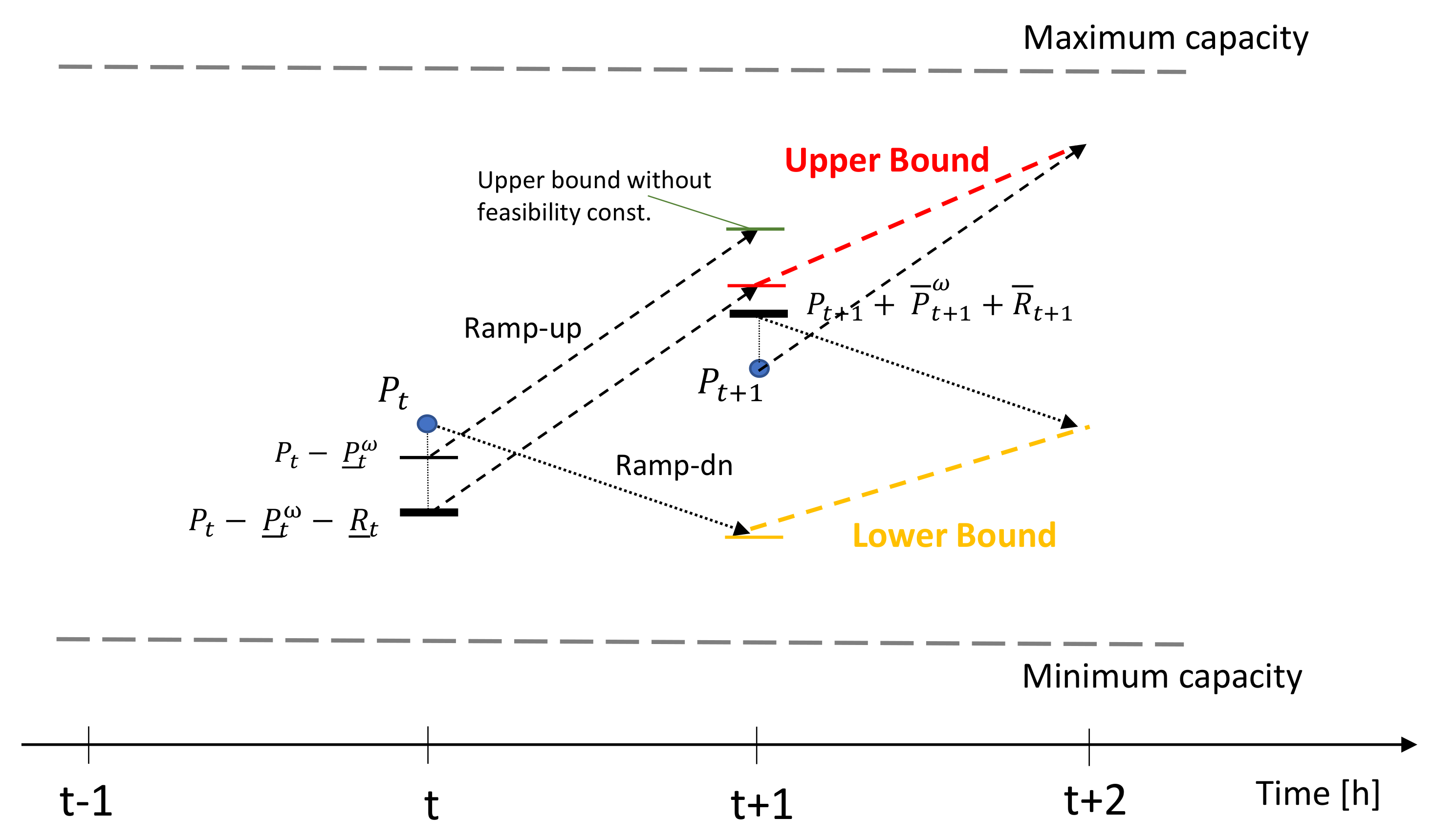
2.3.3. Feasibility of Reserves

The feasibility of reserved capacity is ensured by applying two constraints in the formulation, in which the two constraints consider an actual supply of deployed upward and downward reserves. The constraints (7) and (8) basically represent ramp-up and ramp-down constraints. Additionally, deployed upward and downward reserves are assumed to be supplied, and they are restricted by ramp rates together with supplied power. In particular, the feasibility of the reserve supply is secured by preventing the situation that the downward and upward reserves are deployed by one generator sequentially.

An example to present how the reserve feasibility in ramp constraints is ensured is illustrated in Figure 2. For a scenario $\omega$, the optimal operating point is $P_t - P_t^{\omega }$ at time t, and the deployed downward reserve ${\underline{R}}_t$ is supplied. In this case, $P_{t + 1} + {\overline{P}}_{t + 1}^{\omega } + {\overline{R}}_{t + 1}$ can move up to the red line at time $t + 1$ by the ramp-up rate in (7). However, conventional UC models that do not consider reserve supply allow $P_{t + 1} + {\overline{P}}_{t + 1}^{\omega } + {\overline{R}}_{t + 1}$ to move up to the upper bound shown by the green line at time $t + 1$, where the difference between the red and green upper bounds indicates an infeasible amount to be supplied when the downward reserve at time t is supplied. Consequently, upward reserve or redispatch may not be supplied at time $t + 1$. In this context, the presented ramp constraints considering reserve feasibility avoid the worst case when downward and upward reserves are deployed consecutively and supplied by one generator. Similarly, a lower bound is formed based on Equation (8).

$$\begin{array}{c}{P}_{tc} + {\overline{P}}_{tc}^{\omega } + {\overline{R}}_{tc} - (P_{t - 1,c} - {\underline{P}}_{t - 1,c}^{\omega } - {\underline{R}}_{t - 1,c})\le r{u}_c(U_{tc} - V_{tc}) + s{u}_c·V_{tc,}\end{array}$$

$$\begin{array}{c}\forall \omega \in \mathsf{\Omega },t = 2,3,\dots ,T,\forall c\in {\mathrm{G}}^{\mathrm{c}}\end{array}$$

(7)

$$P_{tc} + {\overline{P}}_{tc}^{\omega } + {\overline{R}}_{tc} - (P_{t + 1,c} - {\underline{P}}_{t + 1,c}^{\omega } - {\underline{R}}_{t + 1,c})\le r{d}_c(U_{tc} - W_{t + 1,c}) + s{d}_c·W_{t + 1,c,}$$

$$\begin{array}{c}\forall \omega \in \mathsf{\Omega },t = 1,2,\dots ,T - 1,\forall c\in {\mathrm{G}}^{\mathrm{c}}\end{array}$$

(8)

The constraints (9)–(12) prevent situations when upward or downward reserves are sequentially deployed and supplied by one generator at time t and $t + 1$. These constraints guarantee the supply of reserves for at least the time t and $t + 1$ when the upward reserves are sequentially deployed by one generator at time t and $t + 1$. The guaranteed time for reserve supply can be extended up to $t + N$.

The available maximum upward reserve at time $t + 1$ when reserve feasibility constraints are applied is illustrated in Figure 3. By considering the actual supply of upward reserve at time t, available upward reserve at $t + 1$ is capped by the maximum capacity limit. Without the feasibility constraints (9) and (11), the upward reserve at time $t + 1$ can be deployed up to “${\overline{R}}_{t + 1}$ without feasibility," and some of them cannot be supplied if the deployed reserve is supplied at time t. Figure 4 also shows the restricted downward reserve at time $t + 1$ by (10) and (12). For scenario $\omega$, the operating point of the generator is $P_t - P_t^{\omega }$ with redispatch at time t when the deployed reserve ${\underline{R}}_t$ is not supplied. The maximum available ${\underline{R}}_{t + 1}$ is represented by “${\underline{R}}_{t + 1}$ with feasibility,” while the maximum available downward reserves at time $t + 1$ with the consideration of reserve supply is smaller than that.

$$\begin{array}{c}{P}_{tc} + {\overline{R}}_{tc} + {\overline{R}}_{t + 1,c}\le g_c^{max}·(U_{tc} + V_{t + 1,c}),t = 1,2,\dots ,T - 1,\forall c\in {\mathrm{G}}^{\mathrm{c}}\end{array}$$

(9)

$$\begin{array}{c}{P}_{tc} - {\underline{R}}_{tc} - {\underline{R}}_{t + 1,c}\ge g_c^{min}·U_{tc} - g_c^{max}·V_{t + 1,c,}t = 1,2,\dots ,T - 1,\forall c\in {\mathrm{G}}^{\mathrm{c}}\end{array}$$

(10)

$$\begin{array}{c}{P}_c^0 + {\overline{R}}_c^0 + {\overline{R}}_{tc}\le g_c^{max}·(u_c^0 + V_{tc}),t = 1,\forall c\in {\mathrm{G}}^{\mathrm{c}}\end{array}$$

(11)

$$\begin{array}{c}{P}_c^0 - {\underline{R}}_c^0 - {\underline{R}}_{tc}\ge g_c^{min}·u_c^0 - g_c^{max}·V_{tc,}t = 1,\forall c\in {\mathrm{G}}^{\mathrm{c}}\end{array}$$

(12)

2.3.4. Maximum Capacity for Generators

The constraints in (13) represent that the sum of power generation, deployed upward reserve, and redispatched power by a conventional generator is less than or equal to the maximum capacity of the generator that is represented by the variable, $Pma{x}_{tc}^{\omega }$. The variable changes based on the operating point in the previous interval and ramp rates. Basically, a conventional generator c has its maximum available capacity, $g_c^{max}$, in (14) when it is turned on. However, that capacity may be a maximum upper bound that cannot be immediately reached by the ramp-up rate. Instead, variable capacity $Pma{x}_{tc}^{\omega }$ that is less than or equal to $g_c^{max}$ can provide a realistic and tight upper bound of the output of the generator in (13) (see, e.g., [7,8]).

$$\begin{array}{c}{P}_{tc} + {\overline{R}}_{tc} + {\overline{P}}_{tc}^{\omega }\le Pma{x}_{tc,}^{\omega }\forall \omega \in \mathsf{\Omega },\forall t\in \mathrm{T},\forall c\in {\mathrm{G}}^{\mathrm{c}}\end{array}$$

(13)

$$\begin{array}{c}Pma{x}_{tc}^{\omega }\le g_c^{max}·U_{tc,}\forall \omega \in \mathsf{\Omega },\forall t\in \mathrm{T},\forall c\in {\mathrm{G}}^{\mathrm{c}}\end{array}$$

(14)

The maximum capacity of a generator changes along with the changes of the generator’s operating point. If the operating point of the generator is supposed to move up to the next operating point at time t from the previous actual operating point, $P_{t - 1,c} + {\overline{P}}_{t - 1,c}^{\omega } - {\underline{P}}_{t - 1,c}^{\omega }$, in the constraints (15), the operating points change based on the ramp-up or start-up rates, depending on the generators’ status. Basically, this type of constraint offers a tight upper bound on the capacity limit and consequently shortens the solution time. In the case that the generator’s operating point moves down at time $t + 1$, the operating point is restricted by the previous operating point and ramp-down or shut-down rate in (16).

$$\begin{array}{c}Pma{x}_{tc}^{\omega }\le P_{t - 1,c} + {\overline{P}}_{t - 1,c}^{\omega } - {\underline{P}}_{t - 1,c}^{\omega } + r{u}_c(U_{tc} - V_{tc}) + s{u}_c·V_{tc},\end{array}$$

$$\begin{array}{c}\forall \omega \in \mathsf{\Omega },t = 2,3,\dots ,T,\forall c\in {\mathrm{G}}^{\mathrm{c}}\end{array}$$

(15)

$$Pma{x}_{tc}^{\omega }\le P_{t + 1,c} + {\overline{P}}_{t + 1,c}^{\omega } - {\underline{P}}_{t + 1,c}^{\omega } + r{d}_c(U_{tc} - W_{t + 1,c}) + s{d}_c·W_{t + 1,c},$$

$$\begin{array}{c}\forall \omega \in \mathsf{\Omega },t = 1,2,\dots ,T - 1,\forall c\in {\mathrm{G}}^{\mathrm{c}}\end{array}$$

(16)

Conventional generators also have minimum capacity limits that ensure stable generation outputs and reasonable production efficiencies. The operating point and downward operating reserve have lower bound constraints based on their minimum output limits, $g_c^{min}$, in (17).

$$\begin{array}{c}{P}_{tc} - {\underline{R}}_{tc} - {\underline{P}}_{tc}^{\omega }\ge g_c^{min}·U_{tc},\forall \omega \in \mathsf{\Omega },\forall t\in \mathrm{T},\forall c\in {\mathrm{G}}^{\mathrm{c}}\end{array}$$

(17)

Available solar PV generation is estimated by randomly generated solar DNI at the second stage and ambient temperature based on a specific solar panel [27,28,29]. In this work, the available power from the solar DNI is calculated every hour. At the second stage, the $|■|$ number of random scenarios for solar power availability are generated, and then electricity generation by solar PV, $P_{ts}$, is limited by the realized solar power availability in (18). The downward redispatch at the second stage cannot be greater than the first-stage dispatch for solar PV systems in (19). The reserve terms do not appear in the formulation because renewable generators are assumed not to provide operating reserves.

$$\begin{array}{c}{P}_{ts} + {\overline{P}}_{ts}^{\omega }\le P_s^{max}\left({\xi }_{\mathsf{s}t}^{\omega }\right),\forall \omega \in \mathsf{\Omega },\forall t\in \mathrm{T},\forall s\in {\mathrm{G}}^{\mathrm{s}}\end{array}$$

(18)

$$\begin{array}{c}{P}_{ts} - {\underline{P}}_{ts}^{\omega }\ge 0,\forall \omega \in \mathsf{\Omega },\forall t\in \mathrm{T},\forall s\in {\mathrm{G}}^{\mathrm{s}}\end{array}$$

(19)

At the second stage, the operating points of wind generators are adjusted with ${\overline{P}}_{tw}^{\omega }$ and ${\underline{P}}_{tw}^{\omega }$ in accordance with their available power, which are referred to as redispatch here. The sum of the operating point determined at the first stage and the amount of upward adjustment cannot exceed the realized wind power availability in (20). The sum of first-stage dispatch and downward redispatch as recourse at the second stage must be non-negative in (21).

$$\begin{array}{c}{P}_{tw} + {\overline{P}}_{tw}^{\omega }\le {\gamma }_w·{\xi }_{\mathsf{w}t,}^{\omega }\forall \omega \in \mathsf{\Omega },\forall t\in \mathrm{T},w\in {\mathrm{G}}^{\mathrm{w}}\end{array}$$

(20)

$$\begin{array}{c}{P}_{tw} - {\underline{P}}_{tw}^{\omega }\ge 0,\forall \omega \in \mathsf{\Omega },\forall t\in \mathrm{T},\forall s\in {\mathrm{G}}^{\mathrm{s}}\end{array}$$

(21)

2.3.5. Start-Up and Shut-Down

Decision variables for commitment, start-up, and shut-down of a conventional generator c at time t are represented by binary variables, which indicate two states, zero or one, in (22). When a generator is committed at time t, the UC decision variable, $U_{tc}$, changes from 0 at time $t - 1$ to 1 at time t; therefore, the start-up and shut-down variables become 1 and 0 at time t, respectively, in (23). Conversely, the shut-down decision variable, $W_{tc}$, becomes 1 when the generator is turned off at time t, and $U_{tc}$ changes from 1 at time $t - 1$ to 0 at time t. The initial commitment status of a generator c is represented by $u_c^0$, which is obtained from the UC solutions in the previous operating period. With $u_c^0$, commitment, start-up, and shut-down status are determined at time $t = 1$ in (24). The sum of the binary decision variables, $V_{tc}$ and $W_{tc}$, cannot be more than 1 in (25), because start-up and shut-down cannot occur simultaneously.

$$\begin{array}{c}{U}_{tc},V_{tc},W_{tc}\in \{0,1\},\forall t\in \mathrm{T},\forall c\in {\mathrm{G}}^{\mathrm{c}}\end{array}$$

(22)

$$\begin{array}{c}{U}_{tc} - U_{t - 1,c} = V_{tc} - W_{tc},t = 2,3,\dots ,T,\forall c\in {\mathrm{G}}^{\mathrm{c}}\end{array}$$

(23)

$$\begin{array}{c}{U}_{tc} - u_c^0 = V_{tc} - W_{tc},t = 1,\forall c\in {\mathrm{G}}^{\mathrm{c}}\end{array}$$

(24)

$$\begin{array}{c}{V}_{tc} + W_{tc}\le 1,\forall t\in \mathrm{T},\forall c\in {\mathrm{G}}^{\mathrm{c}}\end{array}$$

(25)

2.3.6. Minimum Up and Down Times

Thermal generators must remain online for a certain amount of time by (26), once they are committed. Conversely, the generators must stay off for the next several hours when they are turned off, which is a minimum down time constraint represented by (28). Depending on the physical characteristics of the generators, minimum up and down times can range from less than 1 h to more than 10 h. Therefore, (26) enforces the number of time intervals that generators are supposed to be on according to the inherent minimum up time, $u{t}_c^{min}$, once generators are turned on. If the minimum up time is greater than $\left|T\right| - t + 1$, the generator must be online to the end of the operating period.

Constraints (27) ensure that the generators must be turned on for $u{t}_c^{min} - u{t}_c^{sum}$ hours when the generators are turned on $t = 0$. The parameter $u{t}_c^{sum}$ indicates the hours that the generators have been turned on in the previous operating period. In the constraints (27) and (29), $u{t}_c^{sum}$ and $d{t}_c^{sum}$ are calculated at the end of the solution process. For instance, any thermal generator c is on at time $t = \left|T\right|$, the initial on/off state for the next operating period becomes 1 ($u_c^0 = 1$), and the sum of time intervals that the generator has been on is calculated as $u{t}_c^{sum} = {\sum }_{T - u{t}_c^{min} + 1}^T{U}_{tc}$.

$$\begin{array}{c}{V}_{tc}\le U_{\tau c},t = 1,2,\dots ,T - 1,\tau \in [t + 1,min\{t + u{t}_c^{min} - 1,\left|\mathrm{T}\right|\left\}\right],\forall c\in {\mathrm{G}}^{\mathrm{c}}\end{array}$$

(26)

$$\sum _{t = 1}^m{U}_{tc}\ge (u{t}_c^{min} - u{t}_c^{sum})u_c^0,\forall c\in {\mathrm{G}}^{\mathrm{c}},$$

$$\begin{array}{c}\mathrm{where}m = max\{1,min\{\left|\mathrm{T}\right|,u{t}_c^{min} - u{t}_c^{sum}\left\}\right\}\end{array}$$

(27)

$$\begin{array}{c}{W}_{tc}\le 1 - U_{\tau c,}t = 1,2,\dots ,T - 1,\tau \in [t + 1,min\{\left|\mathrm{T}\right|,t + d{t}_c^{min} - 1\left\}\right],\forall c\in {\mathrm{G}}^{\mathrm{c}}\end{array}$$

(28)

$$\sum _{t = 1}^n(1 - U_{tc})\ge min\left\{\right|\mathrm{T}|,(d{t}_c^{min} - d{t}_c^{sum})(1 - u_c^0)\},$$

$$\begin{array}{c}\mathrm{where}n = max\{1,min\{\left|\mathrm{T}\right|,d{t}_c^{min} - d{t}_c^{sum}\left\}\right\},\forall c\in {\mathrm{G}}^{\mathrm{c}}\end{array}$$

(29)

2.3.7. Unserved Demand and Non-Negativity

The constraints (30) restrict unserved demand not to exceed the realized load at d. Continuous decision variables, except the power flows and bus voltage angles, are non-negative by (31).

$$\begin{array}{c}0\le U{D}_{td}^{\omega }\le {\delta }_d·{\xi }_{\mathsf{d}t,}^{\omega }\forall \omega \in \mathsf{\Omega },\forall t\in \mathrm{T},\forall d\in \mathrm{D}\end{array}$$

(30)

$$\begin{array}{c}{P}_{tg},{\overline{P}}_{tg}^{\omega },{\underline{P}}_{tg}^{\omega },{\overline{R}}_{tg},{\underline{R}}_{tg},Pma{x}_{tc}^{\omega }\ge 0\end{array}$$

(31)

2.4. Scenario Generation

Random samples with $\left|\mathrm{T}\right|$ number of time intervals are generated using autoregressive-to-anything (ARTA) processes [30,31,32], where the samples indicate solar DNI, available wind power, and electric load for one day in summer. The historical data used to obtain the ARTA process are from [32,33]. An enhanced method for generating scenarios can improve the accuracy of optimal solutions. The samples are scaled down to meet the capacity of the test system. The 100 generated samples applied to the model are illustrated in Figure 5.

3. Data and Test System

A 24-bus power system is built based on the IEEE 24-bus system [34] for verifying optimal UC solutions, in which eleven thermal generators, five solar PV farms, and six wind farms are located. The total number of transmission lines is thirty eight, with two different voltage levels of 138 kV and 230 kV. The $g_c^{max}$ and $g_c^{min}$ values for renewable resources indicate installed capacity and zero, respectively. Detailed data for the system are listed in Table 1, and the description of the data can be found in Nomenclature.

Table 1. Data of generators in 24-bus test system [34,35].

Gen.	${\mathit{g}}_{\mathit{c}}^{\mathit{min}}$	${\mathit{g}}^{\mathit{max}}$	${\mathit{ut}}_{\mathit{c}}^{\mathit{min}}$	${\mathit{dt}}_{\mathit{c}}^{\mathit{min}}$	${\mathit{ut}}_{\mathit{c}}^{\mathit{sum}}$	${\mathit{dt}}_{\mathit{c}}^{\mathit{sum}}$	${\mathit{u}}_{\mathit{c}}^{\mathbf{0}}$	${\mathit{rd}}_{\mathit{c}}$	${\mathit{ru}}_{\mathit{c}}$	${\mathit{sd}}_{\mathit{c}}$	${\mathit{su}}_{\mathit{c}}$	${\mathit{gcost}}_{\mathit{g}}$	${\mathit{scost}}_{\mathit{c}}$	${\mathit{rucost}}_{\mathit{c}}$	${\mathit{rdcost}}_{\mathit{c}}$
$g_1$	30.4	152	8	4	8	0	1	120	120	120	120	13.32	1430.4	15	14
$g_2$	75	350	8	8	0	2	0	350	350	350	350	20.7	1725	10	9
$g_3$	206.85	591	1	1	0	1	0	240	240	240	240	20.93	3056.7	8	7
$g_4$	12	60	1	1	2	0	1	60	60	60	60	26.11	437	7	5
$g_5$	54.25	155	8	6	0	2	0	155	155	155	155	10.52	312	16	14
$g_6$	54.25	155	8	8	8	0	1	155	155	155	155	10.52	312	16	14
$g_7$	100	400	12	10	3	0	1	80	80	280	280	6.02	0	0	0
$g_8$	100	400	12	10	3	0	1	50	50	280	280	5.47	0	0	0
$g_9$	300	300	1	1	2	0	1	300	300	300	300	19.83	0	0	0
$g_{10}$	108.5	310	8	8	8	0	1	180	180	180	180	10.52	624	17	16
$g_{11}$	140	350	8	8	8	0	1	240	240	240	240	10.89	2298	16	14
$s_1 - s_5$		100
$w_1 - w_6$		100

Table 1. Data of generators in 24-bus test system [34,35].

Gen.	${\mathit{g}}_{\mathit{c}}^{\mathit{min}}$	${\mathit{g}}^{\mathit{max}}$	${\mathit{ut}}_{\mathit{c}}^{\mathit{min}}$	${\mathit{dt}}_{\mathit{c}}^{\mathit{min}}$	${\mathit{ut}}_{\mathit{c}}^{\mathit{sum}}$	${\mathit{dt}}_{\mathit{c}}^{\mathit{sum}}$	${\mathit{u}}_{\mathit{c}}^{\mathbf{0}}$	${\mathit{rd}}_{\mathit{c}}$	${\mathit{ru}}_{\mathit{c}}$	${\mathit{sd}}_{\mathit{c}}$	${\mathit{su}}_{\mathit{c}}$	${\mathit{gcost}}_{\mathit{g}}$	${\mathit{scost}}_{\mathit{c}}$	${\mathit{rucost}}_{\mathit{c}}$	${\mathit{rdcost}}_{\mathit{c}}$
$g_1$	30.4	152	8	4	8	0	1	120	120	120	120	13.32	1430.4	15	14
$g_2$	75	350	8	8	0	2	0	350	350	350	350	20.7	1725	10	9
$g_3$	206.85	591	1	1	0	1	0	240	240	240	240	20.93	3056.7	8	7
$g_4$	12	60	1	1	2	0	1	60	60	60	60	26.11	437	7	5
$g_5$	54.25	155	8	6	0	2	0	155	155	155	155	10.52	312	16	14
$g_6$	54.25	155	8	8	8	0	1	155	155	155	155	10.52	312	16	14
$g_7$	100	400	12	10	3	0	1	80	80	280	280	6.02	0	0	0
$g_8$	100	400	12	10	3	0	1	50	50	280	280	5.47	0	0	0
$g_9$	300	300	1	1	2	0	1	300	300	300	300	19.83	0	0	0
$g_{10}$	108.5	310	8	8	8	0	1	180	180	180	180	10.52	624	17	16
$g_{11}$	140	350	8	8	8	0	1	240	240	240	240	10.89	2298	16	14
$s_1 - s_5$		100
$w_1 - w_6$		100

4. Impacts of Reserve Feasibility Constraints

In this section, optimal upward & downward reserves and UC & ED decisions are presented, which are obtained from the proposed stochastic UC model in Section 2. The impacts on optimal solutions are analyzed when feasibility of reserves is considered. The proposed UC problems are solved by General Algebraic Modeling System (GAMS) 30.3.0 and the MIP solver, CPLEX [36].

4.1. Without Reserve Feasibility

To see how UC and ED solutions are affected by the reserve feasibility constraints, a base case without reserve feasibility is simulated by replacing constraints (7) and (8) with the constraints shown below, in which reserve supply is not considered. Additionally, constraints (9)–(12) are excluded.

$$\begin{array}{c}{P}_{tc} + {\overline{P}}_{tc}^{\omega } - (P_{t - 1,c} - {\underline{P}}_{t - 1,c}^{\omega })\le r{u}_c(U_{tc} - V_{tc}) + s{u}_c·V_{tc,}\end{array}$$

$$\begin{array}{c}\forall \omega \in \mathsf{\Omega },t = 2,3,\dots ,T,\forall c\in {\mathrm{G}}^{\mathrm{c}}\end{array}$$

(32)

$$P_{tc} + {\overline{P}}_{tc}^{\omega } - (P_{t + 1,c} - {\underline{P}}_{t + 1,c}^{\omega })\le r{d}_c(U_{tc} - W_{t + 1,c}) + s{d}_c·W_{t + 1,c,}$$

$$\begin{array}{c}\forall \omega \in \mathsf{\Omega },t = 1,2,\dots ,T - 1,\forall c\in {\mathrm{G}}^{\mathrm{c}}\end{array}$$

(33)

Optimal upward and downward reserve deployments are presented in Figure 6. The costs for reserves are USD 0/MW for generators $g_7$ and $g_8$, and they mainly provide upward and downward reserves. In particular, the downward reserves are mostly deployed by $g_7$ and $g_8$. The thermal generators are assumed to provide upward and downward reserves as much as their maximum capacity and ramp rates allow.

Optimal UC and ED decisions are listed in

Table 2. Optimal unit commitment decisions without considering reserve feasibility.

Unit	Time Interval (h)
	${\mathit{t}}_{\mathbf{1}}$	${\mathit{t}}_{\mathbf{2}}$	${\mathit{t}}_{\mathbf{3}}$	${\mathit{t}}_{\mathbf{4}}$	${\mathit{t}}_{\mathbf{5}}$	${\mathit{t}}_{\mathbf{6}}$	${\mathit{t}}_{\mathbf{7}}$	${\mathit{t}}_{\mathbf{8}}$	${\mathit{t}}_{\mathbf{9}}$	${\mathit{t}}_{\mathbf{10}}$	${\mathit{t}}_{\mathbf{11}}$	${\mathit{t}}_{\mathbf{12}}$	${\mathit{t}}_{\mathbf{13}}$	${\mathit{t}}_{\mathbf{14}}$	${\mathit{t}}_{\mathbf{15}}$	${\mathit{t}}_{\mathbf{16}}$	${\mathit{t}}_{\mathbf{17}}$	${\mathit{t}}_{\mathbf{18}}$	${\mathit{t}}_{\mathbf{19}}$	${\mathit{t}}_{\mathbf{20}}$	${\mathit{t}}_{\mathbf{21}}$	${\mathit{t}}_{\mathbf{22}}$	${\mathit{t}}_{\mathbf{23}}$	${\mathit{t}}_{\mathbf{24}}$
$g_1$	1	1	1	1	1	1	1	1	1	1	1	1	1	1	1	1	1	1	1	1	1	1	1	1
$g_2$	0	0	0	0	0	0	0	0	0	0	0	1	1	1	1	1	1	1	1	1	1	1	1	1
$g_3$	0	0	0	0	0	0	0	0	0	0	0	0	0	1	1	0	0	0	0	0	0	0	0	0
$g_4$	1	1	1	1	0	0	0	0	0	1	1	1	1	1	1	1	1	1	1	1	1	1	1	0
$g_5$	0	0	0	0	1	1	1	1	1	1	1	1	1	1	1	1	1	1	1	1	1	1	1	1
$g_6$	1	1	1	1	1	1	1	1	1	1	1	1	1	1	1	1	1	1	1	1	1	1	1	1
$g_7$	1	1	1	1	1	1	1	1	1	1	1	1	1	1	1	1	1	1	1	1	1	1	1	1
$g_8$	1	1	1	1	1	1	1	1	1	1	1	1	1	1	1	1	1	1	1	1	1	1	1	1
$g_9$	0	0	0	0	0	0	0	0	0	0	0	0	0	0	0	1	1	1	0	0	0	0	0	0
$g_{10}$	1	1	1	1	1	1	1	1	1	1	1	1	1	1	1	1	1	1	1	1	1	1	1	1
$g_{11}$	1	1	1	1	1	1	1	1	1	1	1	1	1	1	1	1	1	1	1	1	1	1	1	1

and

Table 3. Optimal first-stage economic dispatch decisions without considering reserve feasibility.

Unit	Time Interval (h)
	${\mathit{t}}_{\mathbf{1}}$	${\mathit{t}}_{\mathbf{2}}$	${\mathit{t}}_{\mathbf{3}}$	${\mathit{t}}_{\mathbf{4}}$	${\mathit{t}}_{\mathbf{5}}$	${\mathit{t}}_{\mathbf{6}}$	${\mathit{t}}_{\mathbf{7}}$	${\mathit{t}}_{\mathbf{8}}$	${\mathit{t}}_{\mathbf{9}}$	${\mathit{t}}_{\mathbf{10}}$	${\mathit{t}}_{\mathbf{11}}$	${\mathit{t}}_{\mathbf{12}}$	${\mathit{t}}_{\mathbf{13}}$	${\mathit{t}}_{\mathbf{14}}$	${\mathit{t}}_{\mathbf{15}}$	${\mathit{t}}_{\mathbf{16}}$	${\mathit{t}}_{\mathbf{17}}$	${\mathit{t}}_{\mathbf{18}}$	${\mathit{t}}_{\mathbf{19}}$	${\mathit{t}}_{\mathbf{20}}$	${\mathit{t}}_{\mathbf{21}}$	${\mathit{t}}_{\mathbf{22}}$	${\mathit{t}}_{\mathbf{23}}$	${\mathit{t}}_{\mathbf{24}}$
$g_1$	32	32	32	30.4	30.4	30.4	30.4	30.4	30.4	32	58.9	92.9	152	50.8	82.6	32	32	32	150.4	95.4	32	32	30.4	30.4
$g_2$	0	0	0	0	0	0	0	0	0	0	0	75	75	75	75	75	75	75	75	75	75	75	75	75
$g_3$	0	0	0	0	0	0	0	0	0	0	0	0	0	206.9	206.9	0	0	0	0	0	0	0	0	0
$g_4$	12	12	12	12	0	0	0	0	0	12	12	12	12	12	12	12	12	12	12	12	12	12	12	0
$g_5$	0	0	0	0	155	155	155	155	155	155	155	155	155	155	155	155	155	155	155	155	155	155	155	113.9
$g_6$	155	155	155	155	54.3	66.7	82.5	141.2	155	155	155	155	155	155	155	155	155	155	155	155	155	155	119.3	54.3
$g_7$	174.0	187.0	182.9	185.2	183.4	186.4	193.5	198.4	200.2	209.4	195.7	218.8	218.8	218.8	220.3	216.6	214.9	213.1	204.2	204.0	201.9	196.0	189.5	182.6
$g_8$	374.8	350	350	350	350.9	350	350	350	350	350	363.7	350	388.0	354.6	350	350	350	350	363.5	350	350	350	350	350
$g_9$	0	0	0	0	0	0	0	0	0	0	0	0	0	0	0	300	300	300	0	0	0	0	0	0
$g_{10}$	310	310	310	310	292.1	310	310	310	310	310	310	310	310	310	310	310	310	310	310	310	310	310	310	310
$g_{11}$	350	270.4	219.0	175.9	140	140	140	140	186.1	266.5	350	350	350	350	350	310.6	287.1	252.8	350	350	339.0	221.0	140	140
$s_1$	0	0	0	0	0	0	0.1	3.2	9.5	9.9	6.8	4.3	7.5	4.3	0.2	0.2	0.2	3.3	6.4	0.5	0	0	0	0
$s_2$	0	0	0	0	0	0	0.1	3.2	9.5	9.9	6.8	4.3	7.5	4.3	0.2	0.2	0.2	3.3	6.4	0.5	0	0	0	0
$s_3$	0	0	0	0	0	0	0.1	3.2	9.5	9.9	6.8	4.3	7.5	4.3	0.2	0.2	0.2	3.3	6.4	0.5	0	0	0	0
$s_4$	0	0	0	0	0	0	0.1	3.2	9.5	9.9	6.8	4.3	7.5	4.3	0.2	0.2	0.2	3.3	6.4	0.5	0	0	0	0
$s_5$	0	0	0	0	0	0	0.1	3.2	9.5	9.9	6.8	4.3	7.5	4.3	0.2	0.2	0.2	3.3	6.4	0.5	0	0	0	0
$w_1$	5.6	9.3	7.1	6.1	4.4	2.0	1.4	2.4	1.2	6.5	6.1	4.0	2.1	1.7	2.5	1.7	2.6	2.9	4.4	2.9	4.2	5.9	6.9	2.4
$w_2$	5.6	9.3	7.1	6.1	4.4	2.0	1.4	2.4	1.2	6.5	6.1	4.0	2.1	1.7	2.5	1.7	2.6	2.9	4.4	2.9	4.2	5.9	6.9	2.4
$w_3$	5.6	9.3	7.1	6.1	4.4	2.0	1.4	2.4	1.2	6.5	6.1	4.0	2.1	1.7	2.5	1.7	2.6	2.9	4.4	2.9	4.2	5.9	6.9	2.4
$w_4$	5.6	9.3	7.1	6.1	4.4	2.0	1.4	2.4	1.2	6.5	6.1	4.0	2.1	1.7	2.5	1.7	2.6	2.9	4.4	2.9	4.2	5.9	6.9	2.4
$w_5$	5.6	9.3	7.1	6.1	4.4	2.0	1.4	2.4	1.2	6.5	6.1	4.0	2.1	1.7	2.5	1.7	2.6	2.9	4.4	2.9	4.2	5.9	6.9	2.4
$w_6$	5.6	9.3	7.1	6.1	4.4	2.0	1.4	2.4	1.2	6.5	6.1	4.0	2.1	1.7	2.5	1.7	2.6	2.9	4.4	2.9	4.2	5.9	6.9	2.4

. The costs of generator $g_9$ is USD 0/MW for reserve and USD 0/MWh for generation; however, $g_9$ was mostly turned off because of a high minimum output level. The generator $g_5$ has a relatively low generation cost and high ramp rates, so it has a high possibility of being committed. However, it was finally turned on from $t = 5$ by the minimum down-time constraint.

4.2. Reserve Feasibility in Ramp Constraints

The impact of considering reserve supply in the ramp constraints is simulated by applying the constraints (7) and (8) and excluding the constraints (9)–(12). Optimal reserve deployments are illustrated in Figure 7.

Unlike the case shown in Figure 6, $g_8$ is determined not to provide the upward reserve. The total amount of deployed upward reserves by $g_7$ is decreased from 1802.8 MW to 1368.2 MW, which is about a 24% decrement. For downward reserves, deployments decline from 1166.5 MW to 437.6 MW by $g_7$ and from 2871 MW to 1200 MW by $g_8$. The decrements indicate that these amounts of reserves are not feasible by ramp rates when upward and downward reserves are supplied by one generator.

Optimal UC and ED decisions are listed in

Table 4. Optimal unit commitment decisions considering reserves in the ramp constraints.

Unit	Time Interval (h)
	${\mathit{t}}_{\mathbf{1}}$	${\mathit{t}}_{\mathbf{2}}$	${\mathit{t}}_{\mathbf{3}}$	${\mathit{t}}_{\mathbf{4}}$	${\mathit{t}}_{\mathbf{5}}$	${\mathit{t}}_{\mathbf{6}}$	${\mathit{t}}_{\mathbf{7}}$	${\mathit{t}}_{\mathbf{8}}$	${\mathit{t}}_{\mathbf{9}}$	${\mathit{t}}_{\mathbf{10}}$	${\mathit{t}}_{\mathbf{11}}$	${\mathit{t}}_{\mathbf{12}}$	${\mathit{t}}_{\mathbf{13}}$	${\mathit{t}}_{\mathbf{14}}$	${\mathit{t}}_{\mathbf{15}}$	${\mathit{t}}_{\mathbf{16}}$	${\mathit{t}}_{\mathbf{17}}$	${\mathit{t}}_{\mathbf{18}}$	${\mathit{t}}_{\mathbf{19}}$	${\mathit{t}}_{\mathbf{20}}$	${\mathit{t}}_{\mathbf{21}}$	${\mathit{t}}_{\mathbf{22}}$	${\mathit{t}}_{\mathbf{23}}$	${\mathit{t}}_{\mathbf{24}}$
$g_1$	1	1	1	1	1	1	1	1	1	1	1	1	1	1	1	1	1	1	1	1	1	1	1	1
$g_2$	0	0	0	0	0	0	0	0	0	1	1	1	1	1	1	1	1	1	1	1	1	1	1	1
$g_3$	0	0	0	0	0	0	0	0	0	0	0	0	0	0	1	1	1	1	0	0	0	0	0	0
$g_4$	1	1	1	1	1	1	1	1	1	1	1	1	1	1	1	1	1	1	1	1	1	1	1	1
$g_5$	0	0	0	0	1	1	1	1	1	1	1	1	1	1	1	1	1	1	1	1	1	1	1	1
$g_6$	1	1	1	1	1	1	1	1	1	1	1	1	1	1	1	1	1	1	1	1	1	1	1	1
$g_7$	1	1	1	1	1	1	1	1	1	1	1	1	1	1	1	1	1	1	1	1	1	1	1	1
$g_8$	1	1	1	1	1	1	1	1	1	1	1	1	1	1	1	1	1	1	1	1	1	1	1	1
$g_9$	0	0	0	0	0	0	0	0	0	0	0	0	1	1	0	0	0	0	0	0	0	0	0	0
$g_{10}$	1	1	1	1	1	1	1	1	1	1	1	1	1	1	1	1	1	1	1	1	1	1	1	1
$g_{11}$	1	1	1	1	1	1	1	1	1	1	1	1	1	1	1	1	1	1	1	1	1	1	1	1

and

Table 5. Optimal first-stage economic dispatch decisions considering reserves in the ramp constraints.

Unit	Time Interval (h)
	${\mathit{t}}_{\mathbf{1}}$	${\mathit{t}}_{\mathbf{2}}$	${\mathit{t}}_{\mathbf{3}}$	${\mathit{t}}_{\mathbf{4}}$	${\mathit{t}}_{\mathbf{5}}$	${\mathit{t}}_{\mathbf{6}}$	${\mathit{t}}_{\mathbf{7}}$	${\mathit{t}}_{\mathbf{8}}$	${\mathit{t}}_{\mathbf{9}}$	${\mathit{t}}_{\mathbf{10}}$	${\mathit{t}}_{\mathbf{11}}$	${\mathit{t}}_{\mathbf{12}}$	${\mathit{t}}_{\mathbf{13}}$	${\mathit{t}}_{\mathbf{14}}$	${\mathit{t}}_{\mathbf{15}}$	${\mathit{t}}_{\mathbf{16}}$	${\mathit{t}}_{\mathbf{17}}$	${\mathit{t}}_{\mathbf{18}}$	${\mathit{t}}_{\mathbf{19}}$	${\mathit{t}}_{\mathbf{20}}$	${\mathit{t}}_{\mathbf{21}}$	${\mathit{t}}_{\mathbf{22}}$	${\mathit{t}}_{\mathbf{23}}$	${\mathit{t}}_{\mathbf{24}}$
$g_1$	32.0	32.0	32.0	32.0	32.0	30.4	30.4	32.0	30.4	32.0	32.0	47.2	32.0	32.0	32.6	33.3	32.0	32.0	106.4	39.2	32.0	32.0	30.4	30.4
$g_2$	0	0	0	0	0	0	0	0	0	75.0	75.0	75.0	75.0	75.0	75.0	75.0	75.0	75.0	75.0	75.0	75.0	75.0	75.0	75.0
$g_3$	0	0	0	0	0	0	0	0	0	0	0	0	0	0	206.9	206.9	206.9	206.9	0	0	0	0	0	0
$g_4$	12.0	12.0	12.0	12.0	12.0	12.0	12.0	12.0	12.0	12.0	12.0	12.0	12.0	12.0	12.0	12.0	12.0	12.0	12.0	12.0	12.0	12.0	12.0	12.0
$g_5$	0	0	0	0	135.1	155	144.2	155.0	155.0	155.0	155.0	155.0	155.0	155.0	155.0	155.0	155.0	155.0	155.0	155.0	155.0	155.0	155.0	141.4
$g_6$	155.0	155.0	155.0	155.0	54.3	54.3	54.3	88.7	153.1	155.0	155.0	155.0	155.0	155.0	155.0	155.0	155.0	155.0	155.0	155.0	155.0	155.0	115.7	54.3
$g_7$	194.3	197.1	188.3	186.0	183.4	186.4	193.5	198.4	202.0	204.7	209.4	214.5	219.1	221.4	220.3	219.0	216.0	213.7	211.7	213.7	203.2	198.7	185.1	170.3
$g_8$	400.0	400.0	400.0	400.0	400.0	400.0	400.0	400.0	400.0	400.0	400.0	400.0	400.0	400.0	400.0	400.0	400.0	400.0	400.0	400.0	400.0	400.0	378.3	400.0
$g_9$	0	0	0	0	0	0	0	0	0	0	0	0	300.0	300.0	0	0	0	0	0	0	0	0	0	0
$g_{10}$	310.0	310.0	310.0	288.5	249.4	260.5	287.1	298.9	294.1	310.0	310.0	310.0	310.0	310.0	310.0	310.0	310.0	310.0	310.0	310.0	310.0	288.5	288.5	232.9
$g_{11}$	304.5	210.4	163.6	145.0	140.0	140.0	140.0	140.0	140.0	146.3	251.9	350.0	157.7	230.3	350.0	350.0	329.1	295.4	350.0	350.0	287.8	192.5	140.0	140.0
$s_1$	0	0	0	0	0	0	0.1	3.2	9.5	9.9	6.8	4.3	7.5	4.3	0.2	0.2	0.2	3.3	6.4	0.5	0	0	0	0
$s_2$	0	0	0	0	0	0	0.1	3.2	9.5	9.9	6.8	4.3	7.5	4.3	0.2	0.2	0.2	3.3	6.4	0.5	0	0	0	0
$s_3$	0	0	0	0	0	0	0.1	3.2	9.5	9.9	6.8	4.3	7.5	4.3	0.2	0.2	0.2	3.3	6.4	0.5	0	0	0	0
$s_4$	0	0	0	0	0	0	0.1	3.2	9.5	9.9	6.8	4.3	7.5	4.3	0.2	0.2	0.2	3.3	6.4	0.5	0	0	0	0
$s_5$	0	0	0	0	0	0	0.1	3.2	9.5	9.9	6.8	4.3	7.5	4.3	0.2	0.2	0.2	3.3	6.4	0.5	0	0	0	0
$w_1$	5.6	9.3	7.1	6.1	4.4	2.0	1.4	2.4	1.2	6.5	6.1	4.0	2.1	1.7	2.5	1.7	2.6	2.9	4.4	2.9	4.2	5.9	6.9	2.4
$w_2$	5.6	9.3	7.1	6.1	4.4	2.0	1.4	2.4	1.2	6.5	6.1	4.0	2.1	1.7	2.5	1.7	2.6	2.9	4.4	2.9	4.2	5.9	6.9	2.4
$w_3$	5.6	9.3	7.1	6.1	4.4	2.0	1.4	2.4	1.2	6.5	6.1	4.0	2.1	1.7	2.5	1.7	2.6	2.9	4.4	2.9	4.2	5.9	6.9	2.4
$w_4$	5.6	9.3	7.1	6.1	4.4	2.0	1.4	2.4	1.2	6.5	6.1	4.0	2.1	1.7	2.5	1.7	2.6	2.9	4.4	2.9	4.2	5.9	6.9	2.4
$w_5$	5.6	9.3	7.1	6.1	4.4	2.0	1.4	2.4	1.2	6.5	6.1	4.0	2.1	1.7	2.5	1.7	2.6	2.9	4.4	2.9	4.2	5.9	6.9	2.4
$w_6$	5.6	9.3	7.1	6.1	4.4	2.0	1.4	2.4	1.2	6.5	6.1	4.0	2.1	1.7	2.5	1.7	2.6	2.9	4.4	2.9	4.2	5.9	6.9	2.4

. The committed hours of all generators increases from 200 to 209 h during the operating period, and dispatched energy from thermal generators at the first stage also increases from 36,968 MWh to 36,976 MWh. Optimal wind and solar energy generation at the first stage is determined to simply minimize changes in operating points at the second stage because no constraints are implemented to raise renewable energy generation.

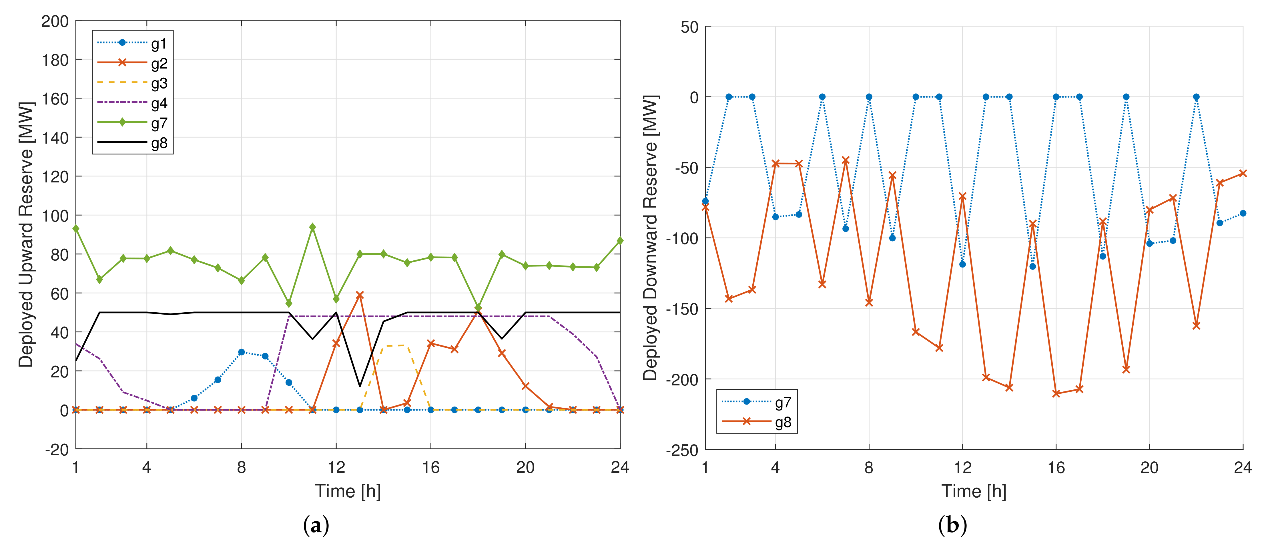
4.3. With Reserve Feasibility Constraints

Optimal reserve deployments are presented in Figure 8 for the case in which the feasibility of reserves is considered in ramp constraints (7) and (8), and $t + 1$ feasibility constraints (9)–(12) are applied to the formulation. The upward reserves are deployed by six thermal generators, and a large portion of reserves are deployed by the generators that have high maximum capacity and ramp-up rates, $g_2$ and $g_3$. The generator $g_7$ provides a 1213 MW upward reserve, which is a decreased amount compared to the case implementing the reserve feasibility in the ramp constraints when the upward and downward reserves are deployed consecutively.

Downward reserves are mostly deployed by generators $g_5$, $g_6$, and $g_8$. The reserve costs for generators $g_5$ and $g_6$ are relatively high compared to $g_7$. However, their generation costs are low, so they are fully dispatched up to their maximum capacity limits while the downward reserves are deployed. Optimal UC and ED decisions are shown in

Table 6. Optimal unit commitment decisions considering feasibility of reserves.

Unit	Time Interval (h)
	${\mathit{t}}_{\mathbf{1}}$	${\mathit{t}}_{\mathbf{2}}$	${\mathit{t}}_{\mathbf{3}}$	${\mathit{t}}_{\mathbf{4}}$	${\mathit{t}}_{\mathbf{5}}$	${\mathit{t}}_{\mathbf{6}}$	${\mathit{t}}_{\mathbf{7}}$	${\mathit{t}}_{\mathbf{8}}$	${\mathit{t}}_{\mathbf{9}}$	${\mathit{t}}_{\mathbf{10}}$	${\mathit{t}}_{\mathbf{11}}$	${\mathit{t}}_{\mathbf{12}}$	${\mathit{t}}_{\mathbf{13}}$	${\mathit{t}}_{\mathbf{14}}$	${\mathit{t}}_{\mathbf{15}}$	${\mathit{t}}_{\mathbf{16}}$	${\mathit{t}}_{\mathbf{17}}$	${\mathit{t}}_{\mathbf{18}}$	${\mathit{t}}_{\mathbf{19}}$	${\mathit{t}}_{\mathbf{20}}$	${\mathit{t}}_{\mathbf{21}}$	${\mathit{t}}_{\mathbf{22}}$	${\mathit{t}}_{\mathbf{23}}$	${\mathit{t}}_{\mathbf{24}}$
$g_1$	1	1	1	1	1	1	1	1	1	1	1	1	1	1	1	1	1	1	1	1	1	1	1	1
$g_2$	0	0	0	0	0	0	0	0	0	0	1	1	1	1	1	1	1	1	1	1	1	1	1	0
$g_3$	1	1	0	0	0	0	0	0	0	0	0	0	1	1	1	1	1	1	0	0	0	0	0	0
$g_4$	1	0	1	1	1	1	1	1	1	1	1	1	1	1	1	1	1	1	1	1	1	1	1	0
$g_5$	0	0	0	0	1	1	1	1	1	1	1	1	1	1	1	1	1	1	1	1	1	1	1	1
$g_6$	1	1	1	1	1	1	1	1	1	1	1	1	1	1	1	1	1	1	1	1	1	1	1	1
$g_7$	1	1	1	1	1	1	1	1	1	1	1	1	1	1	1	1	1	1	1	1	1	1	1	1
$g_8$	1	1	1	1	1	1	1	1	1	1	1	1	1	1	1	1	1	1	1	1	1	1	1	1
$g_9$	0	0	0	0	0	0	0	0	0	0	0	0	0	0	0	0	0	0	0	0	0	0	0	0
$g_{10}$	1	1	1	1	1	1	1	1	1	1	1	1	1	1	1	1	1	1	1	1	1	1	1	1
$g_{11}$	1	1	1	1	1	1	1	1	1	1	1	1	1	1	1	1	1	1	1	1	1	1	1	1

and

Table 7. Optimal first-stage economic dispatch decisions considering feasibility of reserves.

Unit	Time Interval (h)
	${\mathit{t}}_{\mathbf{1}}$	${\mathit{t}}_{\mathbf{2}}$	${\mathit{t}}_{\mathbf{3}}$	${\mathit{t}}_{\mathbf{4}}$	${\mathit{t}}_{\mathbf{5}}$	${\mathit{t}}_{\mathbf{6}}$	${\mathit{t}}_{\mathbf{7}}$	${\mathit{t}}_{\mathbf{8}}$	${\mathit{t}}_{\mathbf{9}}$	${\mathit{t}}_{\mathbf{10}}$	${\mathit{t}}_{\mathbf{11}}$	${\mathit{t}}_{\mathbf{12}}$	${\mathit{t}}_{\mathbf{13}}$	${\mathit{t}}_{\mathbf{14}}$	${\mathit{t}}_{\mathbf{15}}$	${\mathit{t}}_{\mathbf{16}}$	${\mathit{t}}_{\mathbf{17}}$	${\mathit{t}}_{\mathbf{18}}$	${\mathit{t}}_{\mathbf{19}}$	${\mathit{t}}_{\mathbf{20}}$	${\mathit{t}}_{\mathbf{21}}$	${\mathit{t}}_{\mathbf{22}}$	${\mathit{t}}_{\mathbf{23}}$	${\mathit{t}}_{\mathbf{24}}$
$g_1$	30.4	32.0	33.6	32.0	32.0	30.4	30.4	32.0	32.0	32.0	32.0	47.2	30.4	30.4	32.6	33.3	32.0	32.0	106.4	39.2	32.0	32.0	32.0	30.4
$g_2$	0	0	0	0	0	0	0	0	0	0	75.0	75.0	75.0	75.0	75.0	75.0	75.0	75.0	75.0	75.0	75.0	75.0	75.0	0
$g_3$	358.9	206.9	0	0	0	0	0	0	0	0	0	0	206.9	206.9	206.9	206.9	206.9	206.9	0	0	0	0	0	0
$g_4$	12.0	0	12.0	12.0	12.0	12.0	12.0	12.0	12.0	12.0	12.0	12.0	12.0	12.0	12.0	12.0	12.0	12.0	12.0	12.0	12.0	12.0	12.0	0
$g_5$	0	0	0	0	155.0	155.0	155.0	155.0	155.0	155.0	155.0	155.0	155.0	155.0	155.0	155.0	155.0	155.0	155.0	155.0	155.0	155.0	155.0	155.0
$g_6$	134.6	155.0	155.0	155.0	112.2	107.9	124.4	155.0	155.0	155.0	155.0	155.0	155.0	155.0	155.0	155.0	155.0	155.0	155.0	155.0	155.0	155.0	80.3	64.0
$g_7$	181.9	187.0	182.9	185.2	183.4	186.4	193.5	198.4	202.5	204.7	209.4	214.5	219.1	221.4	220.3	219.0	216.0	213.7	211.7	213.7	203.2	198.7	202.2	182.7
$g_8$	350.0	400.0	375.0	400.0	400.0	400.0	400.0	400.0	400.0	400.0	400.0	400.0	400.0	400.0	400.0	400.0	400.0	400.0	400.0	400.0	400.0	400.0	400.0	400.0
$g_9$	0	0	0	0	0	0	0	0	0	0	0	0	0	0	0	0	0	0	0	0	0	0	0	0
$g_{10}$	199.9	130.0	288.5	288.5	171.4	206.8	206.1	232.3	275.5	310.0	310.0	310.0	310.0	310.0	310.0	310.0	310.0	310.0	310.0	310.0	310.0	288.5	284.6	284.0
$g_{11}$	140.0	207.3	214.0	145.8	140.0	140.0	140.0	140.3	154.7	221.3	251.9	350.0	252.4	325.0	350.0	350.0	329.1	295.4	350.0	350.0	287.8	192.5	140.0	140.0
$s_1$	0	0	0	0	0	0	0.1	3.2	9.5	9.9	6.8	4.3	7.5	4.3	0.2	0.2	0.2	3.3	6.4	0.5	0	0	0	0
$s_2$	0	0	0	0	0	0	0.1	3.2	9.5	9.9	6.8	4.3	7.5	4.3	0.2	0.2	0.2	3.3	6.4	0.5	0	0	0	0
$s_3$	0	0	0	0	0	0	0.1	3.2	9.5	9.9	6.8	4.3	7.5	4.3	0.2	0.2	0.2	3.3	6.4	0.5	0	0	0	0
$s_4$	0	0	0	0	0	0	0.1	3.2	9.5	9.9	6.8	4.3	7.5	4.3	0.2	0.2	0.2	3.3	6.4	0.5	0	0	0	0
$s_5$	0	0	0	0	0	0	0.1	3.2	9.5	9.9	6.8	4.3	7.5	4.3	0.2	0.2	0.2	3.3	6.4	0.5	0	0	0	0
$w_1$	5.6	9.3	7.1	6.1	4.4	2.0	1.4	2.4	1.2	6.5	6.1	4.0	2.1	1.7	2.5	1.7	2.6	2.9	4.4	2.9	4.2	5.9	6.9	2.4
$w_2$	5.6	9.3	7.1	6.1	4.4	2.0	1.4	2.4	1.2	6.5	6.1	4.0	2.1	1.7	2.5	1.7	2.6	2.9	4.4	2.9	4.2	5.9	6.9	2.4
$w_3$	5.6	9.3	7.1	6.1	4.4	2.0	1.4	2.4	1.2	6.5	6.1	4.0	2.1	1.7	2.5	1.7	2.6	2.9	4.4	2.9	4.2	5.9	6.9	2.4
$w_4$	5.6	9.3	7.1	6.1	4.4	2.0	1.4	2.4	1.2	6.5	6.1	4.0	2.1	1.7	2.5	1.7	2.6	2.9	4.4	2.9	4.2	5.9	6.9	2.4
$w_5$	5.6	9.3	7.1	6.1	4.4	2.0	1.4	2.4	1.2	6.5	6.1	4.0	2.1	1.7	2.5	1.7	2.6	2.9	4.4	2.9	4.2	5.9	6.9	2.4
$w_6$	5.6	9.3	7.1	6.1	4.4	2.0	1.4	2.4	1.2	6.5	6.1	4.0	2.1	1.7	2.5	1.7	2.6	2.9	4.4	2.9	4.2	5.9	6.9	2.4

. Optimal energy generation by thermal generators is 36,978 MWh, and this value shows that thermal generation is increased compared to the case in which feasibility is considered in the ramp constraints.

4.4. Computational Time

Elapsed times in GAMS to obtain the optimal solutions for the three cases described in Section 4.1, Section 4.2, and Section 4.3 are about 310, 411, and 395 seconds, respectively. The relative optimality criterion for the problems is set to 0.01 throughout the simulations. The elapsed time is relatively short when feasibility constraints are not considered.

5. Discussion

In this paper, a stochastic UC model considering feasibility of upward and downward operating reserves is proposed. The proposed model prevents the worst case in which operating reserves cannot be supplied due to excessive deployments by a limited number of generators.

Feasibility of reserves is ensured by applying two types of constraints that restrict the two worst case: (1) upward and downward reserves are deployed consecutively by one generator and (2) upward or downward reserves are consecutively deployed by one generator. In these two cases, deployed reserves are not guaranteed to be supplied at time $t + 1$ when reserves are supplied from time t. With the reserve feasibility constraints, the number of committed thermal generators increases, and dispatched energy increases. The number of thermal generators that provide reserves is also raised.

The proposed UC formulation provides one set of feasible, optimal solutions which can be provided to system operators as day-ahead schedules with available redispatch and load shedding in real-time. As a future work, the performance of the schedule will be investigated.

References

1. Lowery, P.G. Generating Unit Commitment by Dynamic Programming. IEEE Trans. Power Appar. Syst. 1966, 5, 422–426. [Google Scholar] [CrossRef]
2. Muckstadt, J.A.; Koenig, S.A. An Application of Lagrangian Relaxation to Scheduling in Power-Generation Systems. Oper. Res. 1977, 25, 387–403. [Google Scholar] [CrossRef]
3. Merlin, A.; Sandrin, P. A New Method for Unit Commitment at Electricite De France. IEEE Trans. Power Appar. Syst. 1983, PAS-102, 1218–1225. [Google Scholar] [CrossRef]
4. Baldick, R. The Generalized Unit Commitment Problem. IEEE Trans. Power Syst. 1995, 10, 465–475. [Google Scholar] [CrossRef]
5. Garver, L.L. Power Generation Scheduling by Integer Programming-Development of Theory. Trans. Am. Inst. Electr. Eng. Part III Power Appar. Syst. 1962, 81, 730–734. [Google Scholar] [CrossRef]
6. Frangioni, A.; Gentile, C.; Lacalandra, F. Tighter Approximated MILP Formulations for Unit Commitment Problems. IEEE Trans. Power Syst. 2009, 24, 105–113. [Google Scholar] [CrossRef]
7. Carrion, M.; Arroyo, J. A Computationally Efficient Mixed-Integer Linear Formulation for the Thermal Unit Commitment Problem. IEEE Trans. Power Syst. 2006, 21, 1371–1378. [Google Scholar] [CrossRef]
8. Ostrowski, J.; Anjos, M.F.; Vannelli, A. Tight Mixed Integer Linear Programming Formulations for the Unit Commitment Problem. IEEE Trans. Power Syst. 2012, 27, 39–46. [Google Scholar] [CrossRef]
9. Morales-España, G.; Latorre, J.M.; Ramos, A. Tight and Compact MILP Formulation for the Thermal Unit Commitment Problem. IEEE Trans. Power Syst. 2013, 28, 4897–4908. [Google Scholar] [CrossRef]
10. Wang, Q.; Guan, Y.; Wang, J. A Chance-Constrained Two-Stage Stochastic Program for Unit Commitment with Uncertain Wind Power Output. IEEE Trans. Power Syst. 2012, 27, 206–215. [Google Scholar] [CrossRef]
11. Bertsimas, D.; Litvinov, E.; Sun, X.A.; Zhao, J.; Zheng, T. Adaptive Robust Optimization for the Security Constrained Unit Commitment Problem. IEEE Trans. Power Syst. 2013, 28, 52–63. [Google Scholar] [CrossRef]
12. Nycander, E.; Morales-España, G.; Söder, L. Security constrained unit commitment with continuous time-varying reserves. Electr. Power Syst. Res. 2021, 199, 107276. [Google Scholar] [CrossRef]
13. Hedman, K.W.; Ferris, M.C.; O’Neill, R.P.; Fisher, E.B.; Oren, S.S. Co-Optimization of Generation Unit Commitment and Transmission Switching with N-1 Reliability. IEEE Trans. Power Syst. 2010, 25, 1052–1063. [Google Scholar] [CrossRef]
14. Takriti, S.; Birge, J.R.; Long, E. A stochastic model for the unit commitment problem. IEEE Trans. Power Syst. 1996, 11, 1497–1508. [Google Scholar] [CrossRef]
15. Wu, L.; Shahidehpour, M.; Li, T. Stochastic Security-Constrained Unit Commitment. IEEE Trans. Power Syst. 2007, 22, 800–811. [Google Scholar] [CrossRef]
16. Nowak, M.P.; Römisch, W. Stochastic Lagrangian Relaxation Applied to Power Scheduling in a Hydro-Thermal System under Uncertainty. Ann. Oper. Res. 2000, 100, 251–272. [Google Scholar] [CrossRef]
17. Barth, R.; Brand, H.; Meibom, P.; Weber, C. (Eds.) A stochastic unit-commitment model for the evaluation of the impacts of integration of large amounts of intermittent wind power. In Proceedings of the 2006 International Conference on Probabilistic Methods Applied to Power Systems, Stockholm, Sweden, 11–15 June 2006. [Google Scholar] [CrossRef]
18. Tuohy, A.; Meibom, P.; Denny, E.; O’Malley, M. Unit Commitment for Systems with Significant Wind Penetration. IEEE Trans. Power Syst. 2009, 24, 592–601. [Google Scholar] [CrossRef]
19. Wang, J.; Shahidehpour, M.; Li, Z. Security-Constrained Unit Commitment with Volatile Wind Power Generation. IEEE Trans. Power Syst. 2008, 23, 1319–1327. [Google Scholar] [CrossRef]
20. Papavasiliou, A.; Oren, S.S. Multiarea Stochastic Unit Commitment for High Wind Penetration in a Transmission Constrained Network. Oper. Res. 2013, 61, 578–592. [Google Scholar] [CrossRef]
21. Zhao, C.; Guan, Y. Data-Driven Stochastic Unit Commitment for Integrating Wind Generation. IEEE Trans. Power Syst. 2016, 31, 2587–2596. [Google Scholar] [CrossRef]
22. Street, A.; Oliveira, F.; Arroyo, J.M. Contingency-Constrained Unit Commitment with n-K Security Criterion: A Robust Optimization Approach. IEEE Trans. Power Syst. 2011, 26, 1581–1590. [Google Scholar] [CrossRef]
23. Huang, Y.; Zheng, Q.P.; Wang, J. Two-stage stochastic unit commitment model including non-generation resources with conditional value-at-risk constraints. Electr. Power Syst. Res. 2014, 116, 427–438. [Google Scholar] [CrossRef]
24. Uçkun, C.; Botterud, A.; Birge, J.R. An Improved Stochastic Unit Commitment Formulation to Accommodate Wind Uncertainty. IEEE Trans. Power Syst. 2016, 31, 2507–2517. [Google Scholar] [CrossRef]
25. Birge, J.R.; Louveaux, F. Introduction to Stochastic Programming; Springer: New York, NY, USA, 1997. [Google Scholar]
26. Shapiro, A.; Dentcheva, D.; Ruszczynski, A. Lectures on Stochastic Programming; MPS-SIAM: Philadelphia, PA, USA, 2009. [Google Scholar]
27. Duffie, J.A.; Beckman, W.A. Solar Engineering of Thermal Processes; Wiley: New York, NY, USA, 2013. [Google Scholar]
28. Paatero, J.V.; Lund, P.D. Effects of large-scale photovoltaic power integration on electricity distribution networks. Renew. Energy 2007, 32, 216–234. [Google Scholar] [CrossRef]
29. Muneer, W.; Bhattacharya, K.; Canizares, C.A. Large-Scale Solar PV Investment Models, Tools, and Analysis: The Ontario Case. IEEE Trans. Power Syst. 2011, 26, 2547–2555. [Google Scholar] [CrossRef]
30. Cario, M.C.; Nelson, B.L. Autoregressive to anything: Time-series input processes for simulation. Oper. Res. Lett. 1996, 19, 51–58. [Google Scholar] [CrossRef]
31. Cario, M.C.; Nelson, B.L. Numerical Methods for Fitting and Simulating Autoregressive-to-Anything Processes. INFORMS J. Comput. 1998, 10, 72–81. [Google Scholar] [CrossRef]
32. Park, H. A Stochastic Planning Model for Battery Energy Storage Systems Coupled with Utility-Scale Solar Photovoltaics. Energies 2001, 14, 1244. [Google Scholar] [CrossRef]
33. SolarAnywhere. Available online: https://www.solaranywhere.com/ (accessed on 3 December 2021).
34. Illinois Center for a Smarter Electric Grid (ICSEG). IEEE 24-Bus System. Available online: https://icseg.iti.illinois.edu/ieee-24-bus-system/ (accessed on 3 December 2021).
35. Ordoudis, C.; Pinson, P.; González, J.M.M.; Zugno, M. An Updated Version of the IEEE RTS 24-Bus System for Electricity Market and Power System Operation Studies. Available online: https://orbit.dtu.dk/en/publications/an-updated-version-of-the-ieee-rts-24-bus-system-for-electricity- (accessed on 3 December 2021).
36. GAMS Documentation 33. Available online: https://www.gams.com/latest/docs/S_CPLEX.html (accessed on 3 December 2021).
Figure 1. Decision-making process for the proposed stochastic UC.
Energies 15 06221 g001
Figure 2. Upper and lower bounds for reserves by ramp constraints.
Energies 15 06221 g002
Figure 3. Reserve when upward operating reserves are procured consecutively.
Energies 15 06221 g003
Figure 4. Reserve when downward operating reserves are procured consecutively.
Energies 15 06221 g004
Figure 5. One hundred random samples for a day in summer.
Energies 15 06221 g005
Figure 6. Optimal reserve deployments when the feasibility constraints are not implemented. (a) Upward operating reserve; (b) Downward operating reserve.
Energies 15 06221 g006
Figure 7. Optimal reserve deployments when reserves are considered in the ramp constraint: (a) upward operating reserve; (b) downward operating reserve.
Energies 15 06221 g007
Figure 8. Optimal reserve deployments when reserve feasibility is considered: (a) upward operating reserve, (b) downward operating reserve.
Energies 15 06221 g008