Article

Robust Voltage Control of a Buck DC-DC Converter: A Sliding Mode Approach

1
Physic Department, High School of Engineers of Tunis, Tunis 1008, Tunisia
2
Electrical Department, National Engineering School of Gabes, Zrig Eddakhlania 6029, Tunisia
*
Author to whom correspondence should be addressed.
Energies 2022, 15(17), 6128; https://doi.org/10.3390/en15176128
Submission received: 15 June 2022 / Revised: 22 July 2022 / Accepted: 28 July 2022 / Published: 24 August 2022
(This article belongs to the Special Issue Electrical Power Engineering and Renewable Energy Technologies)

Abstract

:
This paper deals with voltage control in a buck DC-DC converter. In fact, dynamic mathematical equations describing the principle behavior of the above system have been derived. Due to the nonlinearity of the established model, a nonlinear control algorithm is adopted. It is based on the sliding mode control approach. To highlight the performance of the latter, a comparative study with four control algorithms is carried out. The validity of the model and the performance of the conceived algorithms are verified in simulation. Both the system and the algorithm controls are implemented in the Matlab/Simulink environment. Extensive results under different operational conditions are presented and discussed.

1. Introduction

Energy production is one of the most important development priorities. On the one hand, it has been observed that the world’s electrical energy consumption is rapidly increasing [1,2,3,4,5,6,7,8,9]. On the other hand, energy production uses fossil fuels [10,11,12,13] such as oil, coal, and natural gas. They are all burnt and used as energy sources for production. The use of fossil fuels can help to offset the energy demand. However, there is too much carbon dioxide (CO2) in the atmosphere, which can lead to big problems both for people and the earth. This forces humans to seek out alternative energy sources that may be capable of saving both people and the planet.
Many alternative sources are suggested. Among these sources, renewable energy is the most commonly used one. Nowadays, photovoltaic solar energy [14,15,16] and wind energy have become the most used alternative energy sources. The operating power of both the photovoltaic generator and the wind energy sources depends on metrological conditions such as temperature, irradiation, wind speed, etc. [17,18,19,20,21]. The optimal use of the produced energy can be assumed only if the produced wind and photovoltaic sources’ maximum power are extracted and tracked for any change in the metrological conditions. Tools to track these specific points are required [22,23,24,25,26,27].
Most of the proposed power point tracking algorithms are based on varying the generator characteristics in such a way as to be adapted to the latter of the load. The generator characteristic changes are assumed by using a DC-DC converter and a maximum power point tracking (MPPT) algorithm [28,29,30]. Different DC-DC converters are used as buck converters, boost converters, buck–boost converters, etc. [31,32,33,34]. The boost and buck converters are the most commonly used. The buck DC-DC converter is used especially in DC link control, as the DC voltage of the photovoltaic/wind conversion system output depends on the metrological conditions. DC-DC converters are naturally classified as nonlinear systems due to their commuting properties. They are the most commonly used circuits in power electronics, especially in DC link voltage stabilization.
In general, the DC link voltage must be fixed at a desired value despite input voltage and load variations [35]. To regulate the DC voltage magnitude, and obtain a constant and stable output voltage and fast response, many types of controllers are used [27], such as fuzzy logic, PI controllers, PID controllers, sliding mode control, etc. Conventional controllers are in general conceived by using small signal state equations obtained at a specific operation point. The conceived control algorithm remains efficient only around the specified operating point. To avoid the drawbacks of conventional controllers, nonlinear control approaches are investigated and used in the control voltage loop of the buck DC-DC converter. Among these nonlinear control algorithms, the sliding mode approach is the most used. Different sliding mode algorithms, both for continuous and discrete times, are proposed in the literature [36,37,38,39,40,41,42,43]. In [36], a cascade loop control is proposed. The voltage control loop is based on a classical PID controller, and the current loop control is based on zero order sliding mode control over a continuous time. The validity of the conceived algorithm is confirmed under different working conditions, including target voltage variation, load variation and input voltage variations. In [37], a sliding mode controlled pole is conceived both in voltage and current control loops. An integral switching surface is used here. Simulation results are given under target voltage variation and load variation. The fractional order sliding mode is also used in the literature [38]. Different sliding mode approaches for discrete time are used. In fact, in [39], discrete time sliding mode control is investigated for the output voltage control. The performance of the used algorithm is tested only for a fixed target output voltage. Discrete time fast terminal sliding mode control with mismatched disturbance is conceived for DC-DC buck converters, and the control strategy is investigated in [40]. The validity of the proposed algorithm, both in simulation and experimentation, is assessed under both load variations and fluctuations in the input voltage. A discrete repetitive adaptive sliding mode control for the DC-DC buck converter under only variable target output voltage perturbed with a Gaussian noise is conceived in [41]. Simulation results under fixed target voltage and load variations are given. An Adaptive Global Sliding Mode Controller based on the Lyapunov approach is designed for perturbed DC-DC buck converters [42]. In this work, the external disturbances and dynamic uncertainties are modeled with a sinusoidal function. In [43,44], to cope with the chattering problem, a high-order sliding mode control of the DC-DC buck converter is conceived. Practical results under target output voltage variation are presented. In most of the mentioned studies, the performance of the conceived algorithms is validated against external disturbances as input voltage and load variations. The internal disturbances in terms of DC-DC buck converter parameter variations are omitted. Thus, in this paper, we are interested in the performance of the first-order sliding mode in DC-DC buck output voltage control with both external and internal disturbances. Besides this, to highlight the good performance of the investigated control algorithm, a comparison study with four control algorithms is carried out.
The paper is organized as follows. Section 2 presents the modeling of the buck DC-DC converter feeding a resistive load. Section 3 describes the sliding mode controller principle and its application in buck DC-DC converter output voltage control. Section 4 presents the internal model controller. The fuzzy logic controller is given in Section 5. Section 6 illustrates the obtained results in simulation, both for internal and external disturbances. Section 5 concludes the work and presents some suggested prospects.

2. Modelling of DC-DC Buck Converter Mathematical

The synoptic scheme of the DC-DC buck converter is depicted in Figure 1. It consists of an on and off controlled semiconductor (Transistor IGBT, T), a natural commuted semiconductor (Diode, D), a smoothing current system (inductor, L), and a smoothing voltage system (capacitor, C). It is powered by a direct current voltage source and feeds a resistive load.

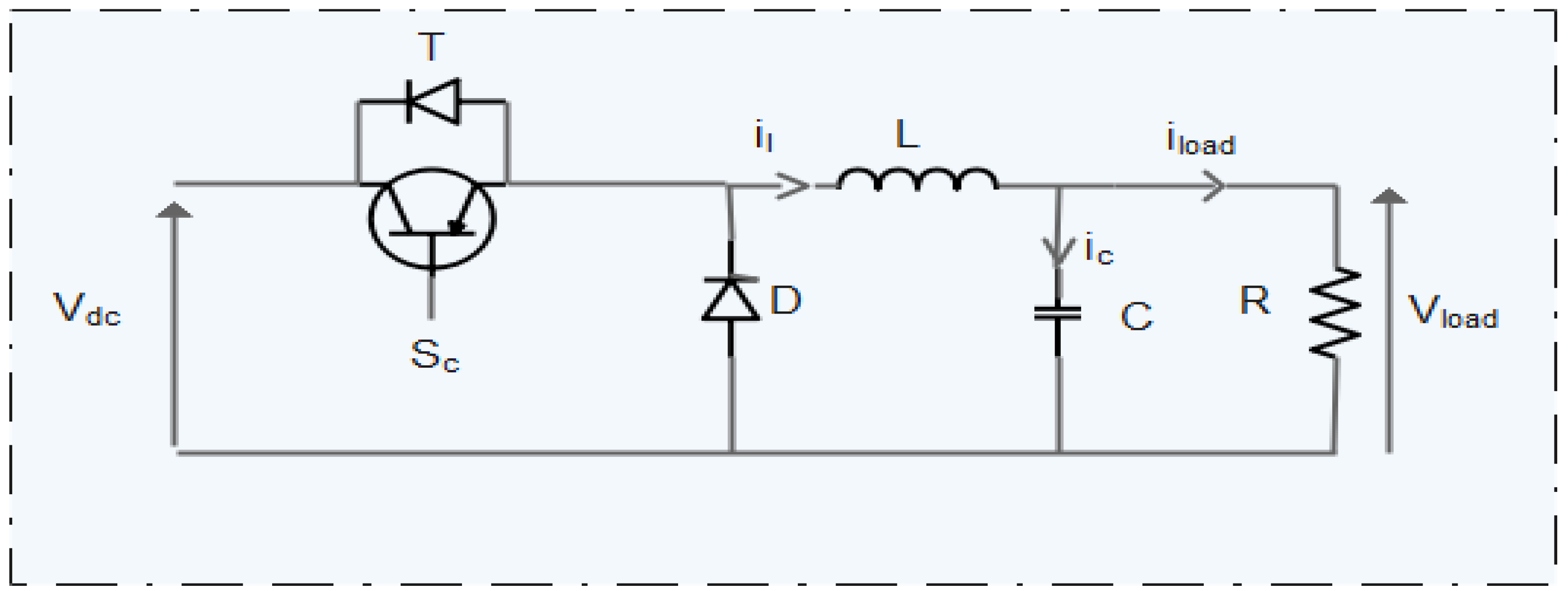
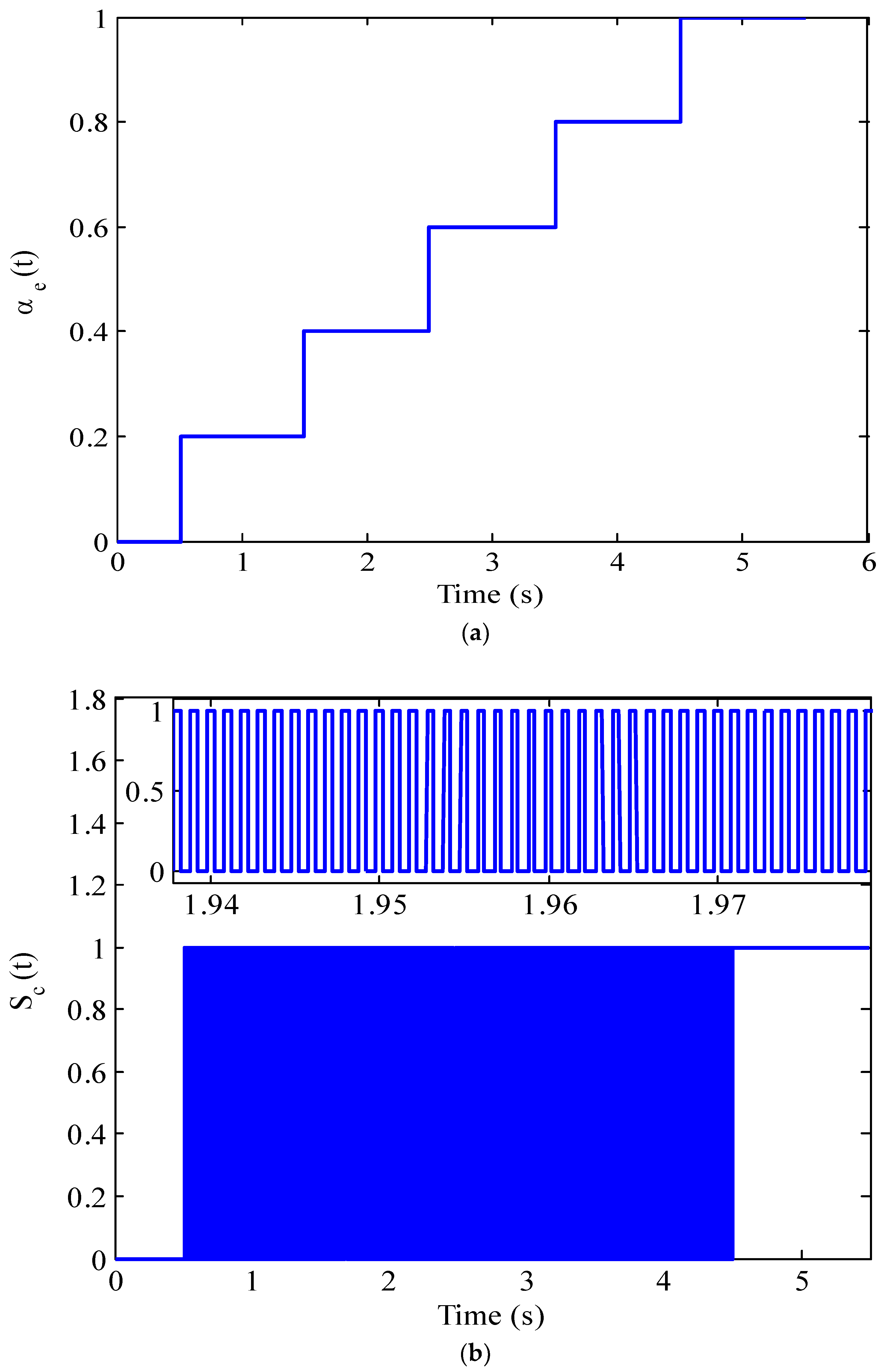
2.1. Bilinear Switching Model of DC-DC Buck Converter

The working principle is based on two alternative phenomena: charging and discharging, based on the control signal state, Sc. When considering the continuous conduction mode and the control signal state levels, two modes are to be considered [45,46,47,48,49,50,51,52,53].
Mode 1:
For the ON mode in which Sc = 1, the transistor T is closed and the diode D is open. Based on Kirchhoff’s current and voltage laws, we can write:
d i l d t = V d c L V l o a d L d V l o a d d t = i l C i l o a d C
Mode2:
Sc = 0, the transistor T becomes open and the diode D begins closed. The state equations describing the inductor current and the output voltage dynamics are given in (2).
d i l d t = V l o a d L d V l o a d d t = i l C i l o a d C
The combination of the two sub models leads to the general buck DC-DC converter model, as illustrated in (3).
d i l d t = S c V d c L V l o a d L d V l o a d d t = i l C i l o a d C
For a resistive load, (3) begins
d i l d t = S c V d c L V l o a d L d V l o a d d t = i l C V l o a d R C

2.2. Averaged Dynamic Model of DC-DC Buck Converter

By using the state-space averaging method [46], Equation (4) can be written as illustrated with Equation (5).
d i l T s d t = S c T s V d c T s L V l o a d T s L d V l o a d T s d t = i l T s C V l o a d T s R C
where i l T s , V l o a d T s , S c T s and V d c T s are the averaged values of inductor current, output voltage, control signal, and input voltage, respectively, in a switching period T s .
This can be put into the more compact form of an uncertain nonlinear system, as indicated by (6).
X ˙ = f X + g X α
The nonlinear equations f X and g X , and averaged state vector X , are defined as follows:
g X = V d c L 0
f X = 0 V l o a d L i l C V l o a d R C
X = i l T s   V l o a d T s T
Here, α is the duty cycle.

2.3. Small Signal Dynamic Model of DC-DC Buck Converter

The small signal DC-DC buck converter model is obtained by linearizing the averaged model around an operating point. Thus, the input control and the output signals’ expressions are to be represented by the sum of their quiescent values and a small alternative current (AC) variation. So, we can write,
i l T s = I l + i ˜ l
V l o a d T s = U l o a d + V ˜ l o a d
V d c T s = U d c + V ˜ d c
S c T s = α e + α ˜
where I l , U l o a d , U d c and α e are the inductor current, the load voltage, the input voltage, and the duty cycle at the operating point, respectively.
Replacing i l T s , V d c T s , V l o a d T s and S c T s with their expressions, Equation (5) begins
d I l + i ˜ l d t = α e + α ˜ U d c + V ˜ d c L U l o a d + V ˜ l o a d L d U l o a d + V ˜ l o a d d t = I l + i ˜ l C U l o a d + V ˜ l o a d R C
By separating steady state terms and small-signal terms, we obtain
d i ˜ d t + d I l d t = α e U d c L U l o a d L D C   t e r m + α V ˜ d c L + α ˜ U d c L V ˜ l o a d L 1 s t   o r d e r   A C   t e r m + α ˜ V ˜ d c L 2 n d   o r d e r   A C   t e r m d V ˜ l o a d d t + d U l o a d d t = I l C U l o a d R C D C   t e r m + i ˜ l C V ˜ l o a d R C 1 s t   o r d e r   A C   t e r m
In the system of Equation (15), the DC terms contain the DC terms only, the first-order AC term contains a product of a DC term with an AC term, and the second order AC term contains a product between two AC terms.
The second-order AC terms are much smaller in magnitude than the firs- order AC terms. Therefore, the second small AC quantity is neglected. Moreover, U d c , I l and U l o a d are constant DC terms. As a result, the sum of the DC term and its derivative are zero. Consequently, only the linear term remains, and the small signal dynamic DC-DC buck converter is defined with (16).
d i ˜ l d t = α ˜ U d c L V ˜ l o a d L d V ˜ l o a d d t = i ˜ l C V ˜ l o a d R C

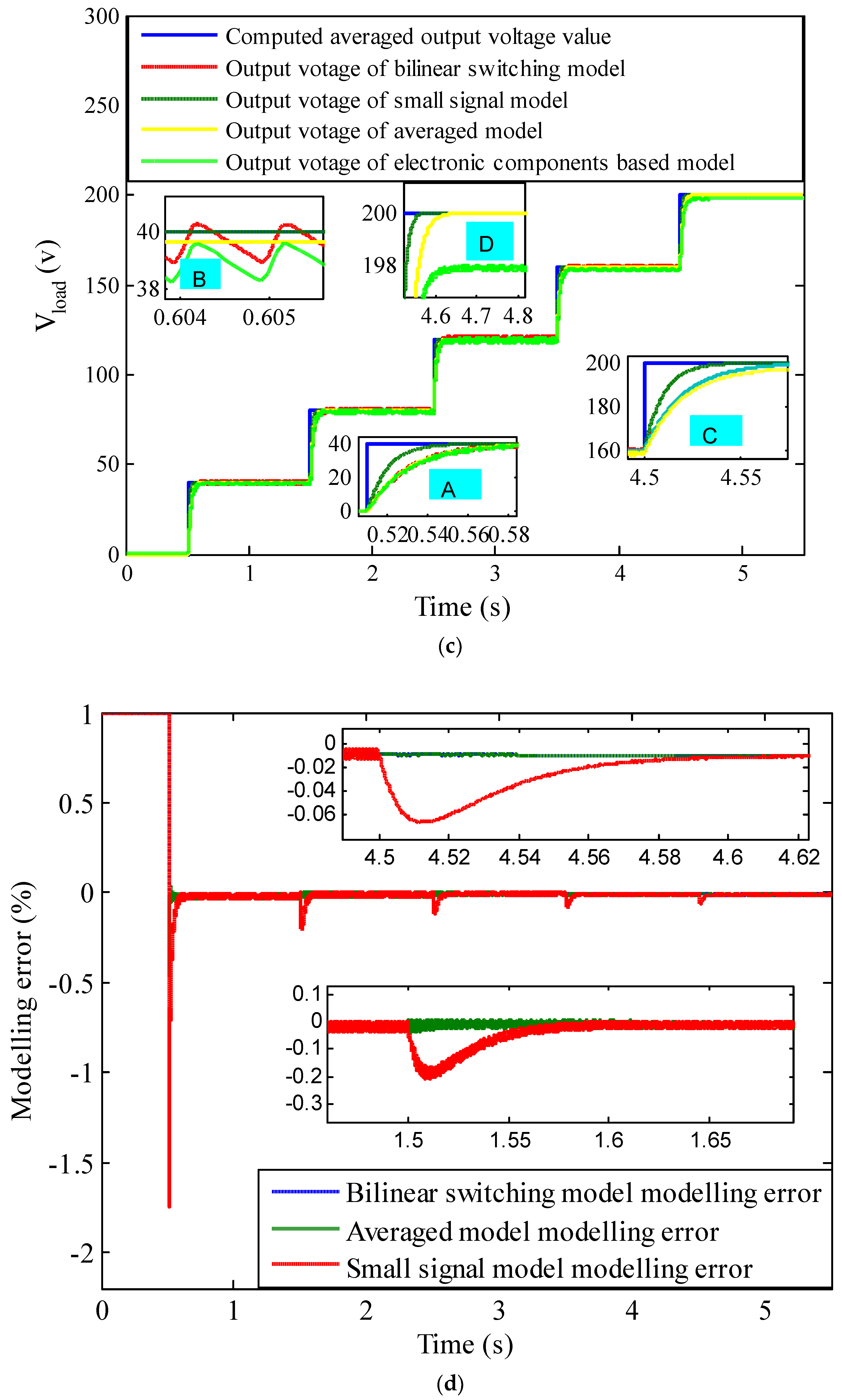
2.4. Comparative Study

To assess the performance of the used mathematical model of the DC-DC buck converter, the three developed models are implemented in Matlab/Simulink platform and compared to one that was established using the predefined electronic components in matlab/Simulink packages. The parameters of the used DC-DC buck converter are grouped in Table 1.
In order to assess the validity of the established models, various operating points are considered. The most significant simulation results are displayed and commented on. Figure 2a shows the evolution of the duty cycle used as a control signal for the averaged and small-signal models. The switching signal obtained at the pulse width modulation bloc, as a control signal for the bilinear switching model and established using the predefined electronic components, is depicted in Figure 2b. Output voltage waveforms are given in Figure 2c. Both dynamic and steady-state working modes are considered. As shown in Figure 2c, output voltage ripples are omitted both for the small signal model and the averaged model, and appear for the switching model, as established using the predefined electronic components in the matlab/Simulink packages. The accuracy of the established model is proven as the modeling error is a few percentage points lower at high duty cycle values, and increases at low duty cycle values, according to the losses in the used power semi-conductors in the DC-DC buck (Figure 2d). Consequently, to cope with the nonlinearities and modeling error, a robust nonlinear control law is to be used. This allows us to use the sliding model approach for DC-DC buck converter control.

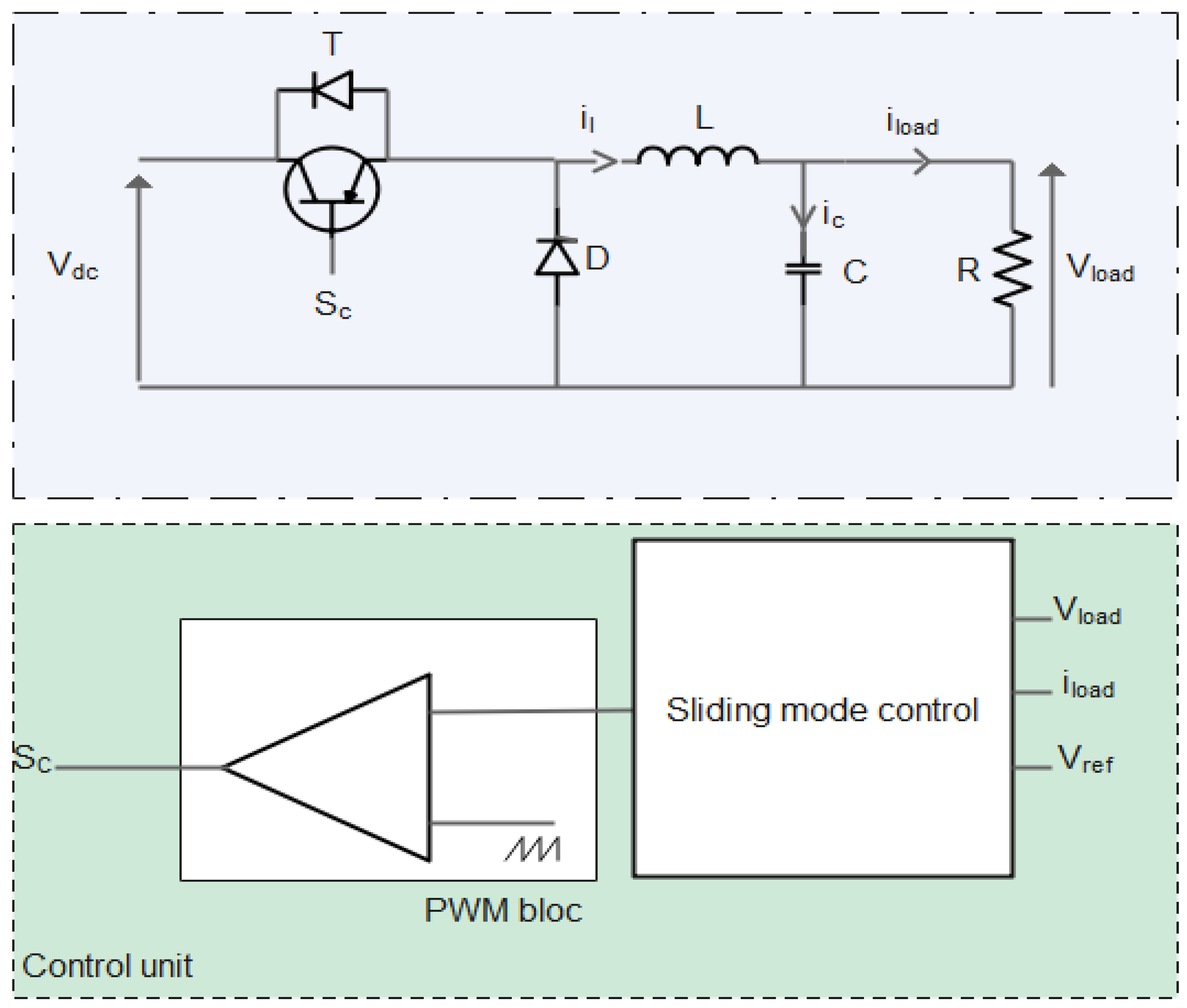
3. Sliding Mode Control Approach for Buck Converter Voltage Control

Control of nonlinear systems using a sliding mode approach was conceived in 1992 by Vadim Ulkin [54] in order to solve the conventional controller’s problems. Typical sliding-mode control operates in the form of these two modes. The first is named the “approaching mode”. When this mode is reached, the convergence of the system state to a predefined manifold called the sliding mode surface in finite time is assumed. The second, designed with sliding mode, follows the sliding surface and returns to the origin. Many approaches to sliding mode control have been conceived. The equivalent control approach [54,55,56,57,58,59] is the most commonly used. Let us denote with S the sliding mode function. In this case, the output’s voltage is controlled. A linear sliding mode surface is adopted. It is defined for the first sliding mode control as follows:
S = C 1 e + e ˙
Here e is the output voltage error and e ˙ is its derivative value.
The output voltage error is defined by (13).
e = V l o a d r e f V l o a d
e ˙ = 1 C i l     V l o a d R
Substituting e and e ˙ with their expressions, the sliding mode surface becomes:
S = 1 C i l + 1 R C C 1 V l o a d + C 1 V l o a d r e f
Its derivative is defined by (21).
S ˙ = 1 C 1 R C R C 2 i l L R 2 C C 1 R C L R 2 C 2 L V l o a d α V d c L C
The equivalent control α e q is deduced from the following equality.
S ˙ = 0
It is defined as:
α e q = L C 1 R C L R C V d c i l L R 2 C C 1 R C L R 2 C V d c V l o a d
Since the duty cycle must be in 0 1 , the real control signal is given by (24).
α ( t ) = 1 s i α ( t ) > 1 α e q + M s i g n ( S ) 0 α ( t ) 1 0 α ( t ) < 0

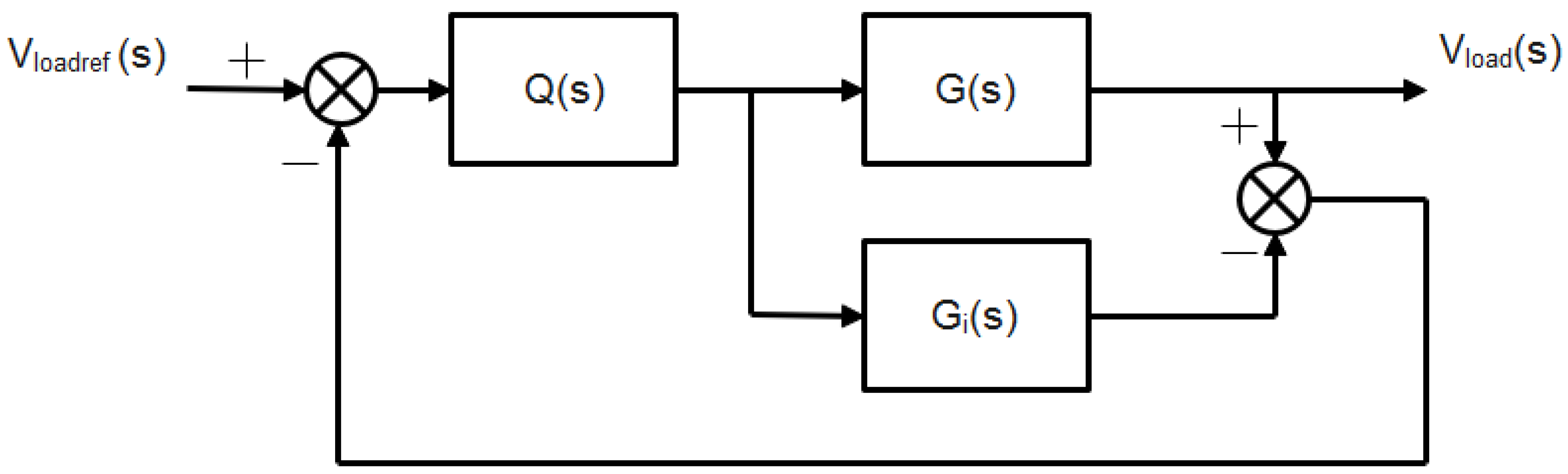
4. Internal Model Control Approach for Buck Converter Voltage Control

The general block diagram of the internal model control (IMC) loop is given in Figure 3. G(s) is the real system’s open loop transfer function, Gi(s) is the system model’s open loop transfer function, and Q(s) is the IMC controller’s transfer function [60].
Referring to Figure 3, we can write
V l o a d = G ( s ) 1 + Q ( s ) G ( s ) G i ( s ) 1 Q ( s ) V l o a d r e f
When the modeling system is perfect, we can write
V l o a d = G ( s ) Q ( s ) V l o a d r e f
The closed loop is stable if and only if G(s) and Q(s) are stable. However, if G(s) is in the non-minimum phase, G−1(s) is not stable. Besides this, if the G−1(s) numerator degree is higher than the denominator degree, then G−1(s) cannot be implemented. Referring to the H2 optimization leads to choosing Q(s) = G−1(s). To assume the feasibility condition, a low-pass filter is added. The final expression of the IMC controller is given in (27).
Q ( s ) = a s + a G 1 ( s )
where a is the filter parameter.

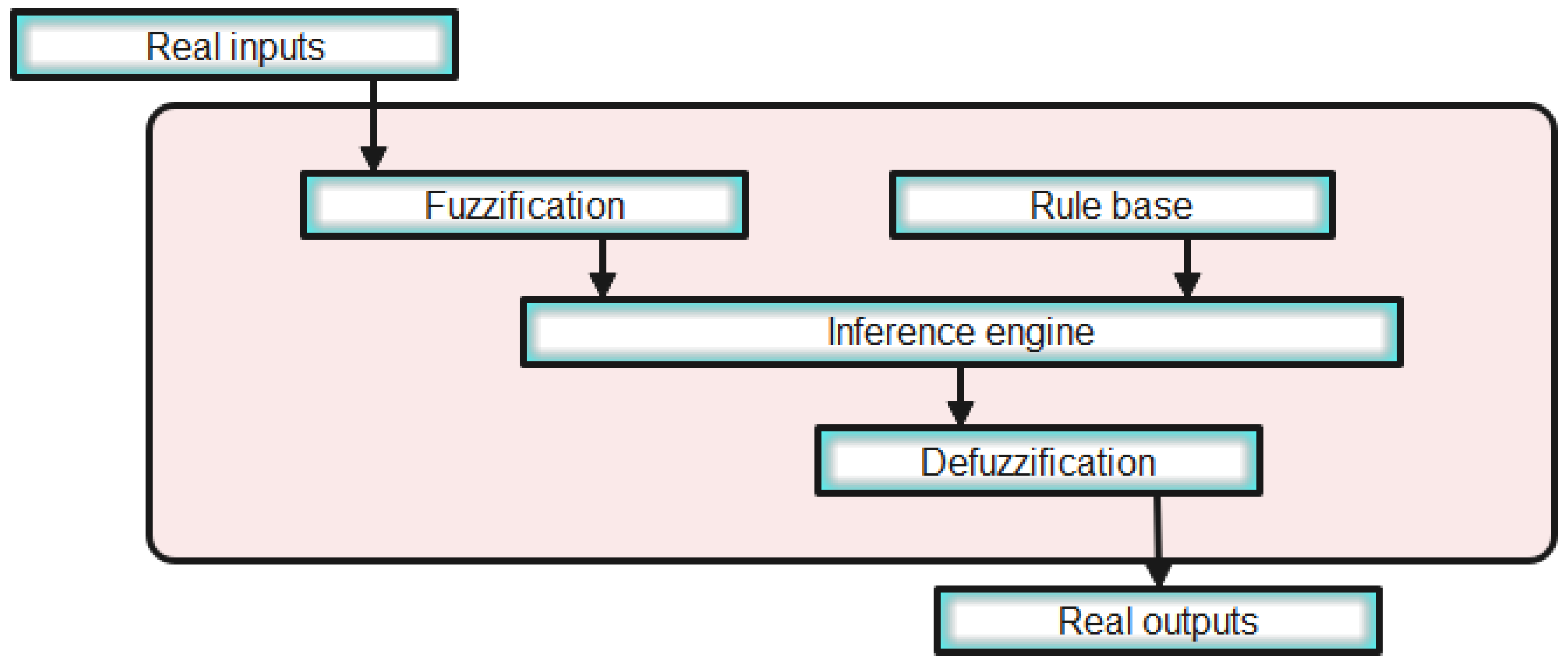
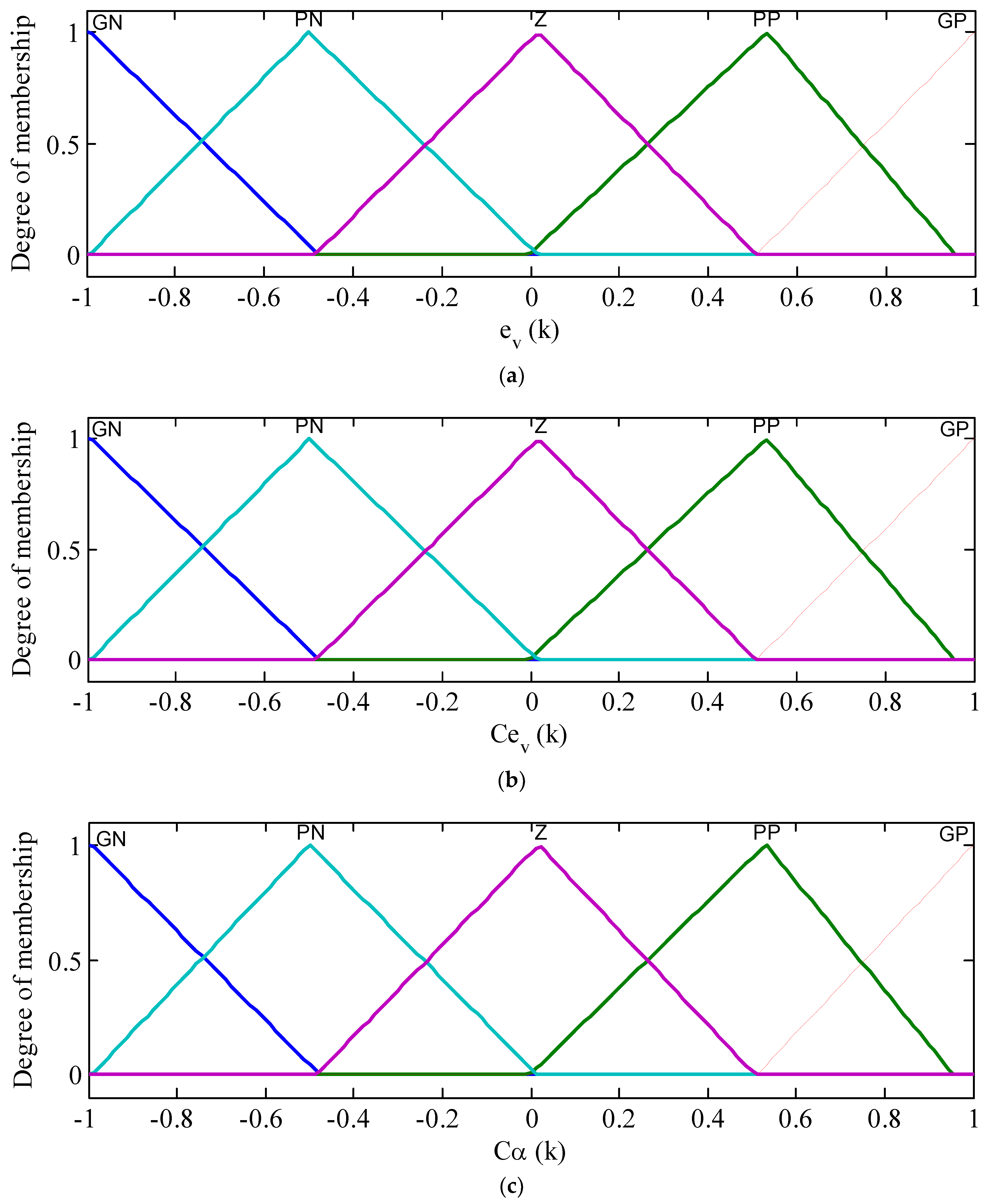
5. Fuzzy Logic for Buck Converter Voltage Control

Fuzzy logic is a computational approach based on degrees of truth. It was first discovered in the 1960s by Lotfi Zadeh [61]. Since the above approach does not require a mathematical model, and is based on human decision-making, this approach can present high efficiency. A mamdani-type fuzzy logic is used for the voltage control. In this fuzzy logic controller (FLC), the voltage error ev(k) and the change in voltage error cev(k) are the inputs of the fuzzy system, while the change in the duty cycle (k) is considered as the output of this system.
The equations for ev(k) and cev(k) are as follows:
e v ( k ) = V l o a d ( k ) V l o a d r e f ( k )
When the modeling system is perfect, we can write
c e v ( k ) = e v ( k ) e v ( k 1 ) T e
where T e is the sample time.
According to Figure 4, three essential steps are to be followed in the mamdani system’s conception. At the fuzification step, the crisp variables ev(k), Cev(k) and (k) are converted to fuzzy sets using triangular membership functions, as can be seen in Figure 5a, b and c, respectively. The linguistic variables GN, PN, Z, PP and GP indicate negative big, negative small, zero, positive small and positive big. The number and the type of the membership function used for the system variables are determined through a trial and error test. The obtained fuzzy output variables are then processed by an inference engine. A sum-prod inference algorithm is adopted in this work. Based on the input membership functions number, the number of rules is obtained. The if–then rules that map input to output are conceived as indicated in Table 2. At the defuzzification step, the inference engine output variable is converted into a crisp value. The centroid defuzzification algorithm is used in this paper. The control signal to be applied in the real system is obtained using a recurrent equation, as indicated in (30).
α ( k ) = α ( k + 1 ) + A C α ( k )
A is adjustable positive gain.

6. Simulation Results

To highlight the effectiveness and robustness of the proposed output voltage controller for the DC-DC buck converter, the overall drive scheme illustrated in Figure 6 was implemented in the Matlab/Simulink environment. Different scenarios were simulated in which the conceived algorithm was evaluated in comparison with four control algorithms: PI, IP, FLC, and IMC. Five scenarios, including abrupt target output voltage variation, triangular target output voltage variation, abrupt input voltage variation, abrupt load variation, and DC-DC buck converter parameter variation, are considered.

6.1. Sliding Mode Parameter Choice

The performance of the conceived sliding mode controller depends on the discontinuous term coefficient. A simulation study was carried out to determine the best choice of this factor. Figure 7 shows the obtained results. It should be noted that high sliding mode parameters lead to reduced response times both for the system and the controller outputs as shown in the zones 1 to 4. On the other hand, it increases the magnitude of oscillation both in the controller and the system responses, which may lead to disrupting the system. Thus, in this work, the considered parameters are chosen in such a way that a compromise between rapidity and stability is achieved.

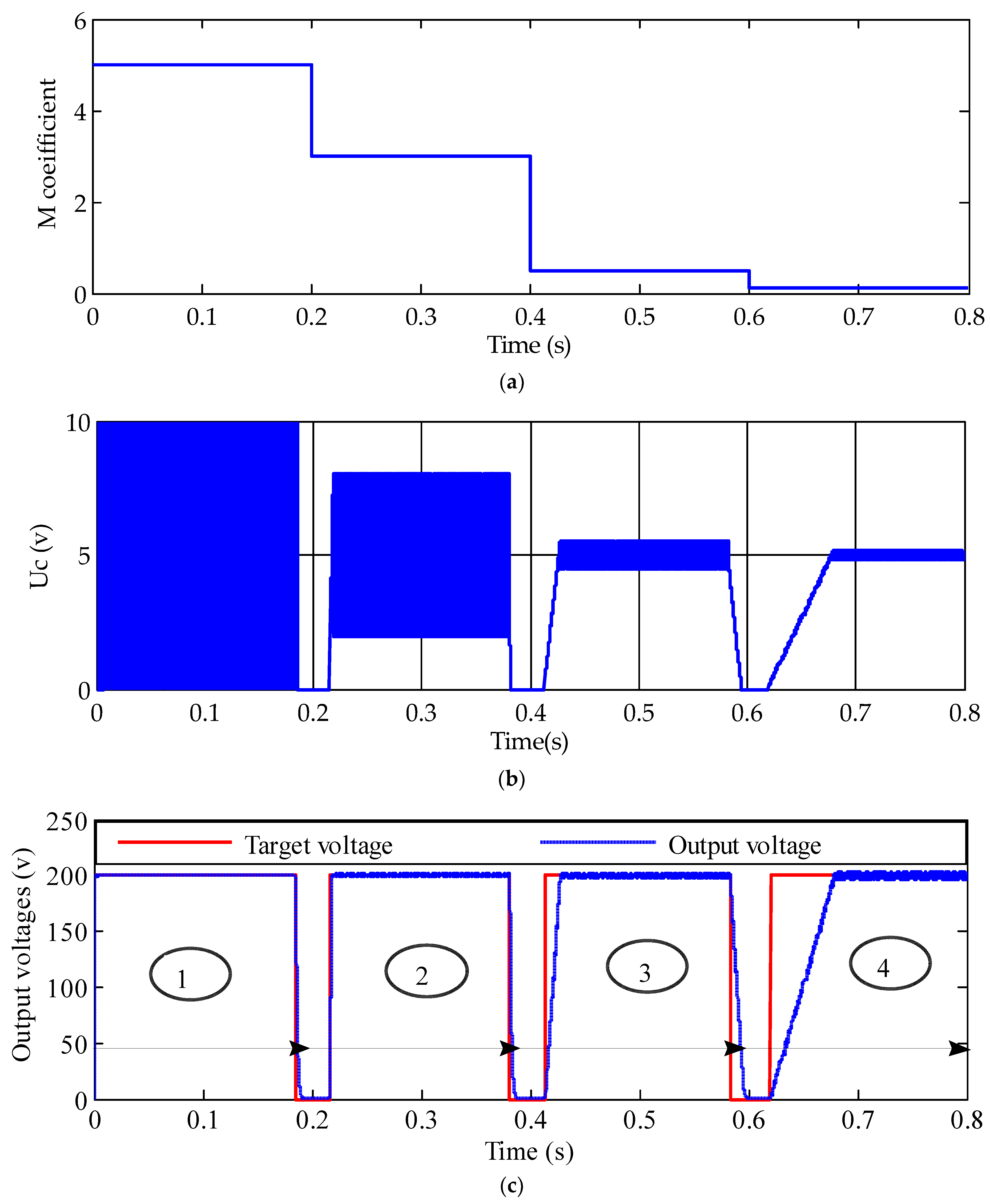
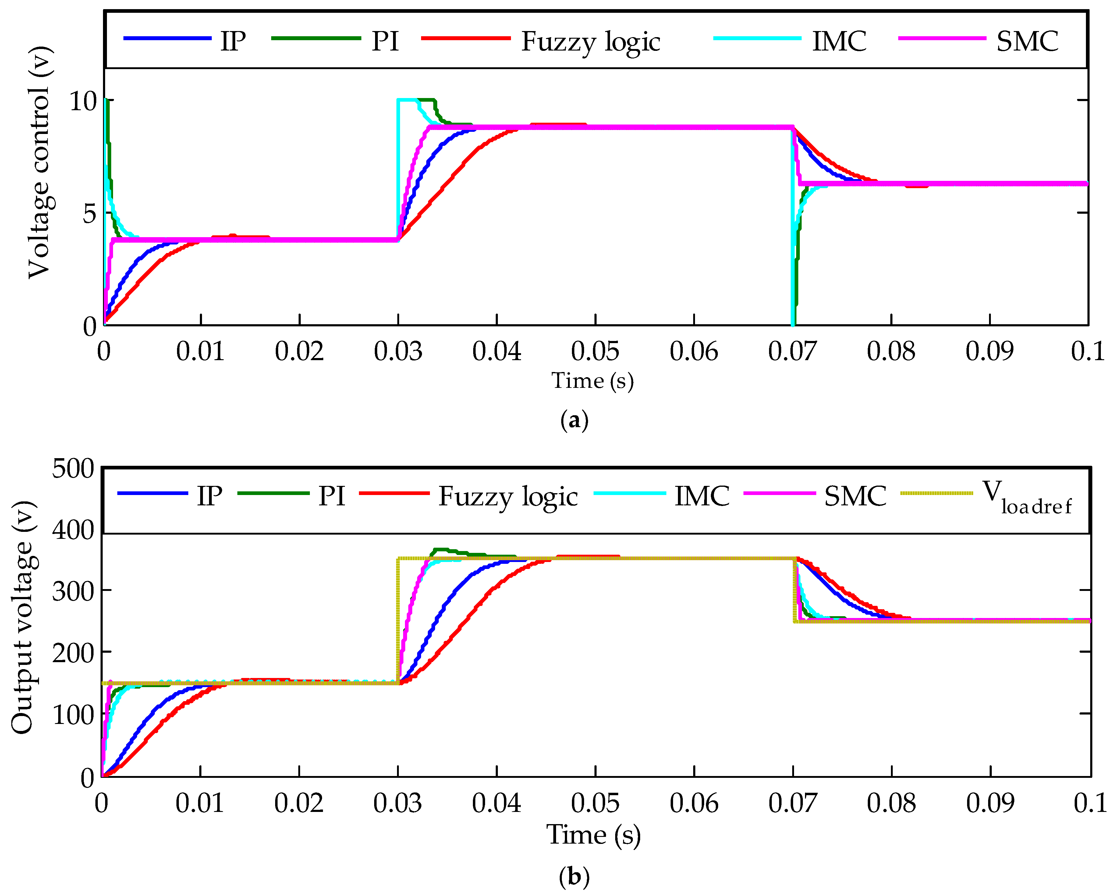
6.2. Controller’s Behavior under Abrupt Target Output Voltage Variations

In this case, the aim is to test the tracking behavior of the proposed sliding mode controller against abrupt target output voltage variations. All five algorithms are implemented and simulated in the same test conditions. In fact, the load resistor, the input voltage, and the DC-DC buck converter parameters are all maintained at their nominal values. The target output voltage is first fixed at 150 v. At t = 0.03 s, it changes to 350 v and decreases to 250 v at t = 0.07 s. The five obtained output voltages and control signals are respectively reported in Figure 8a,b. Comparative performances are extracted and summarized in Table 3.

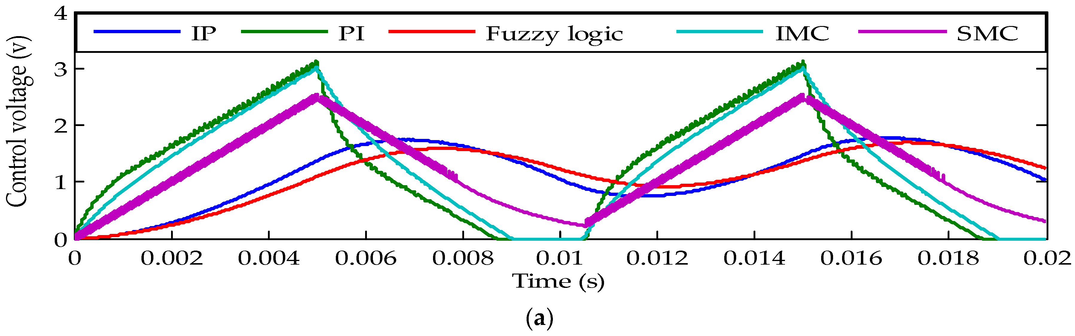
6.3. Controller’s Behavior under Triangular Target Output Voltage Variations

In order to access the dynamic response of the proposed control algorithm, the target output is rapidly changed as a triangular signal is chosen for the five control algorithms. The obtained results are obtained as recorded in Figure 9. Comparative performances in this case are extracted and grouped in Table 3.

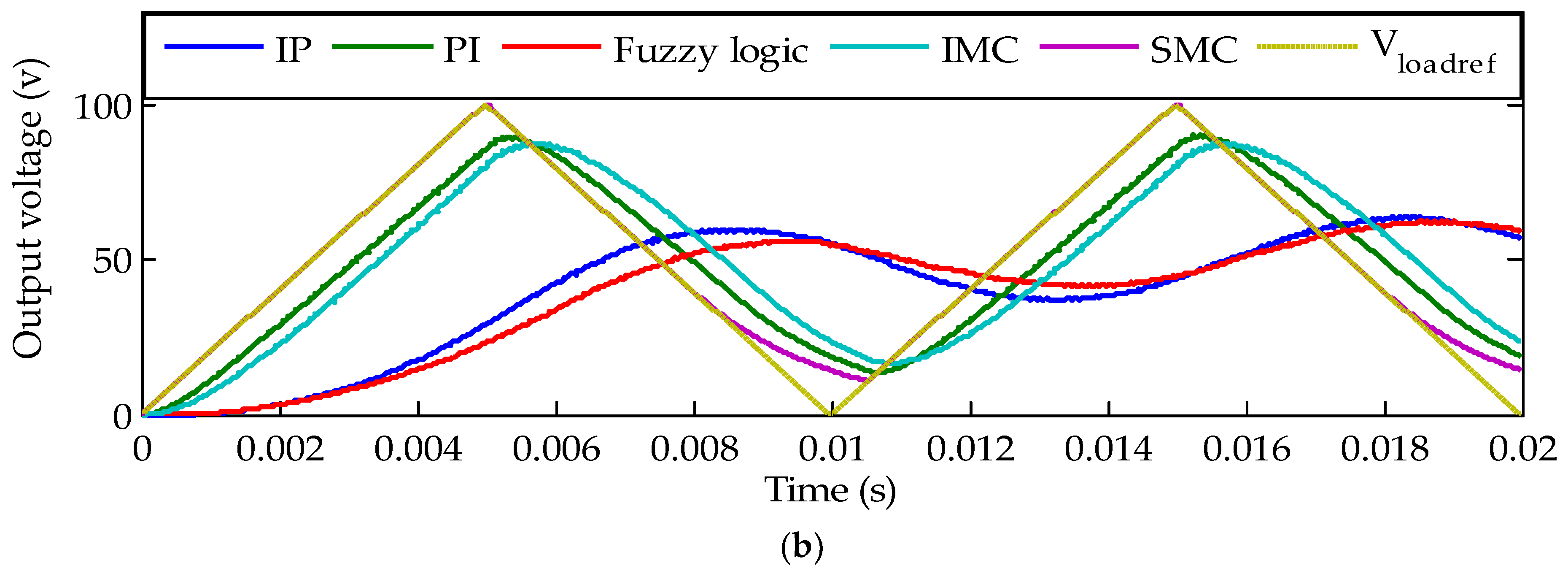
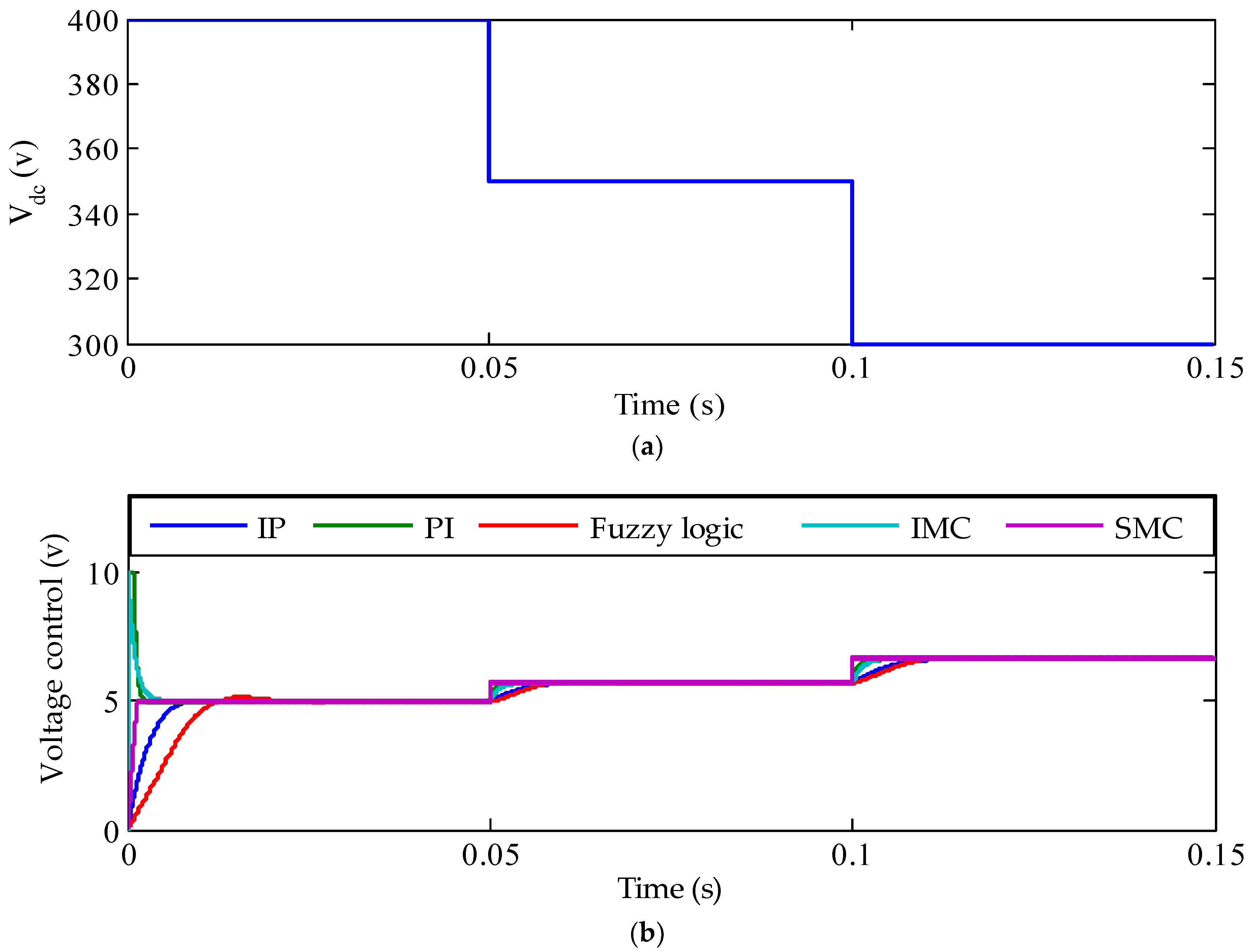
6.4. Controller’s Behavior under Input Voltage Variations

The DC input voltage variations for the five control algorithms are represented in Figure 10. For this test case, the load resistor and the DC-DC buck converter parameters are all maintained at their nominal values. The DC input voltage is fixed at 400 v, and decreased to 350 v and 300 v at t = 0.05 s and t = 0.1 s, respectively. Comparative performances are extracted as represented in Table 3.

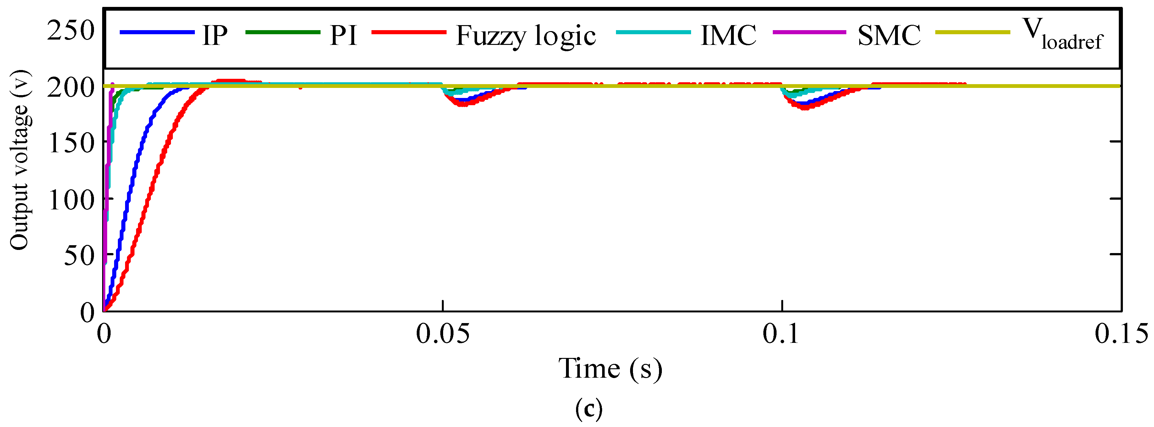
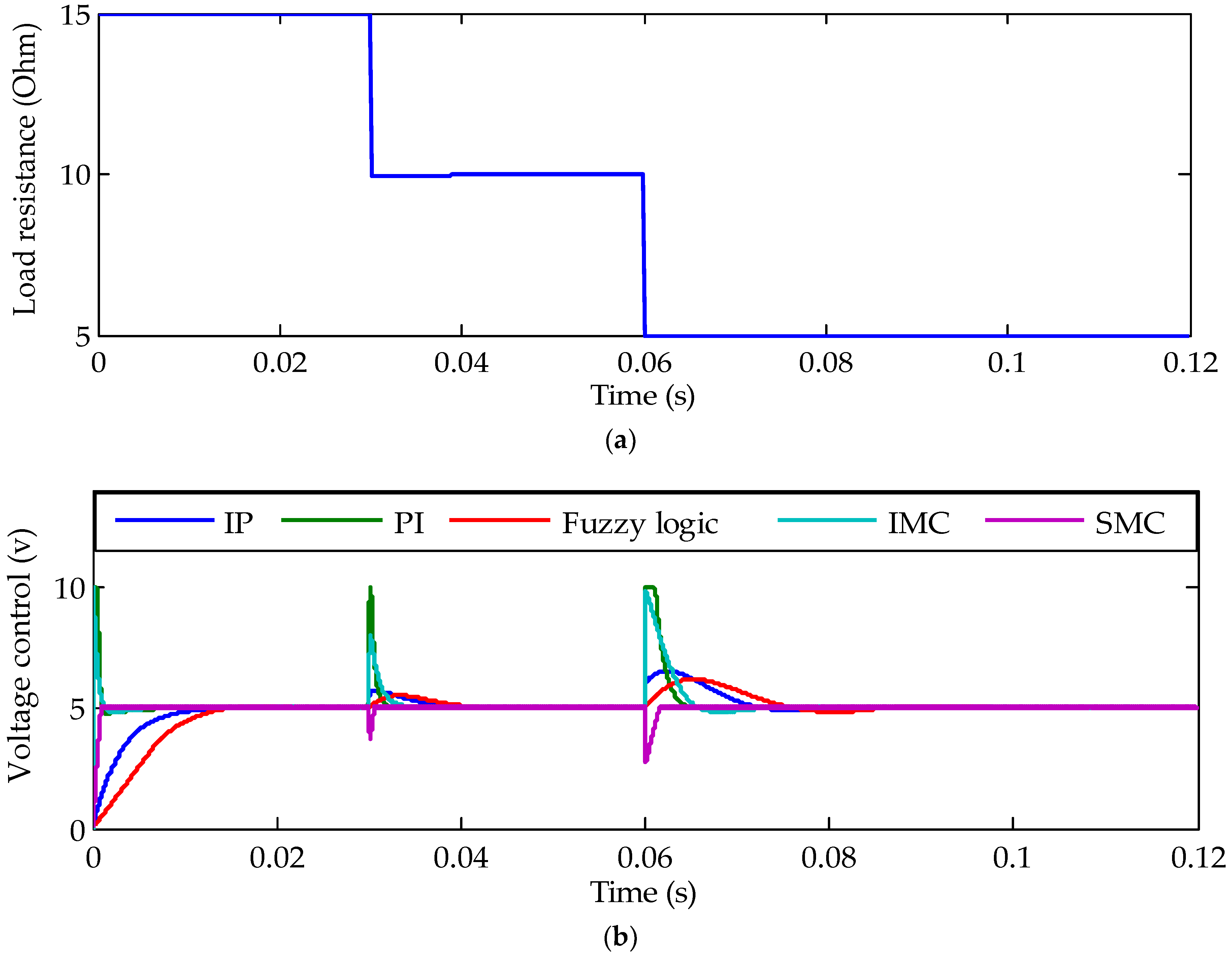
6.5. Controller’s Behavior under Resistor Load Variations

In this test, the input DC voltage and the DC-DC buck converter are held constant at their nominal values. The target output voltage is also fixed to a constant value. The load variation trajectory is given in Figure 11a. The obtained responses of the five algorithms are shown in Figure 11b,c. Table 3 gives the comparison performances in this case.

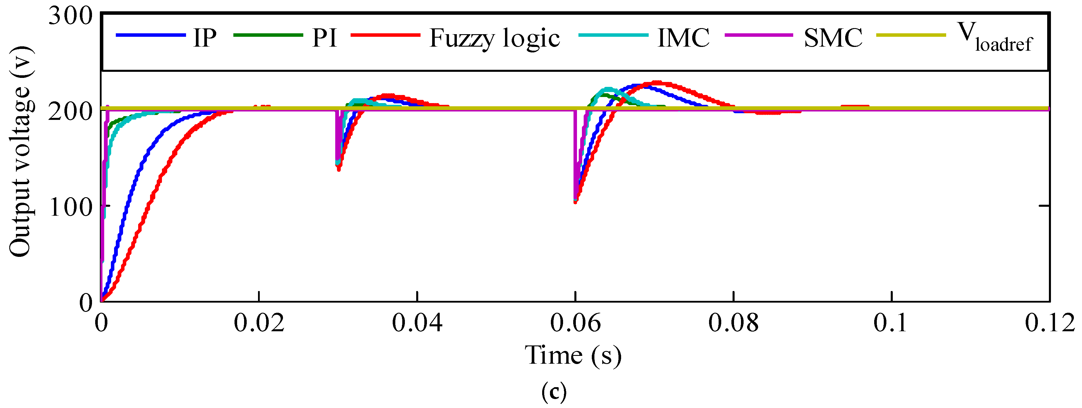
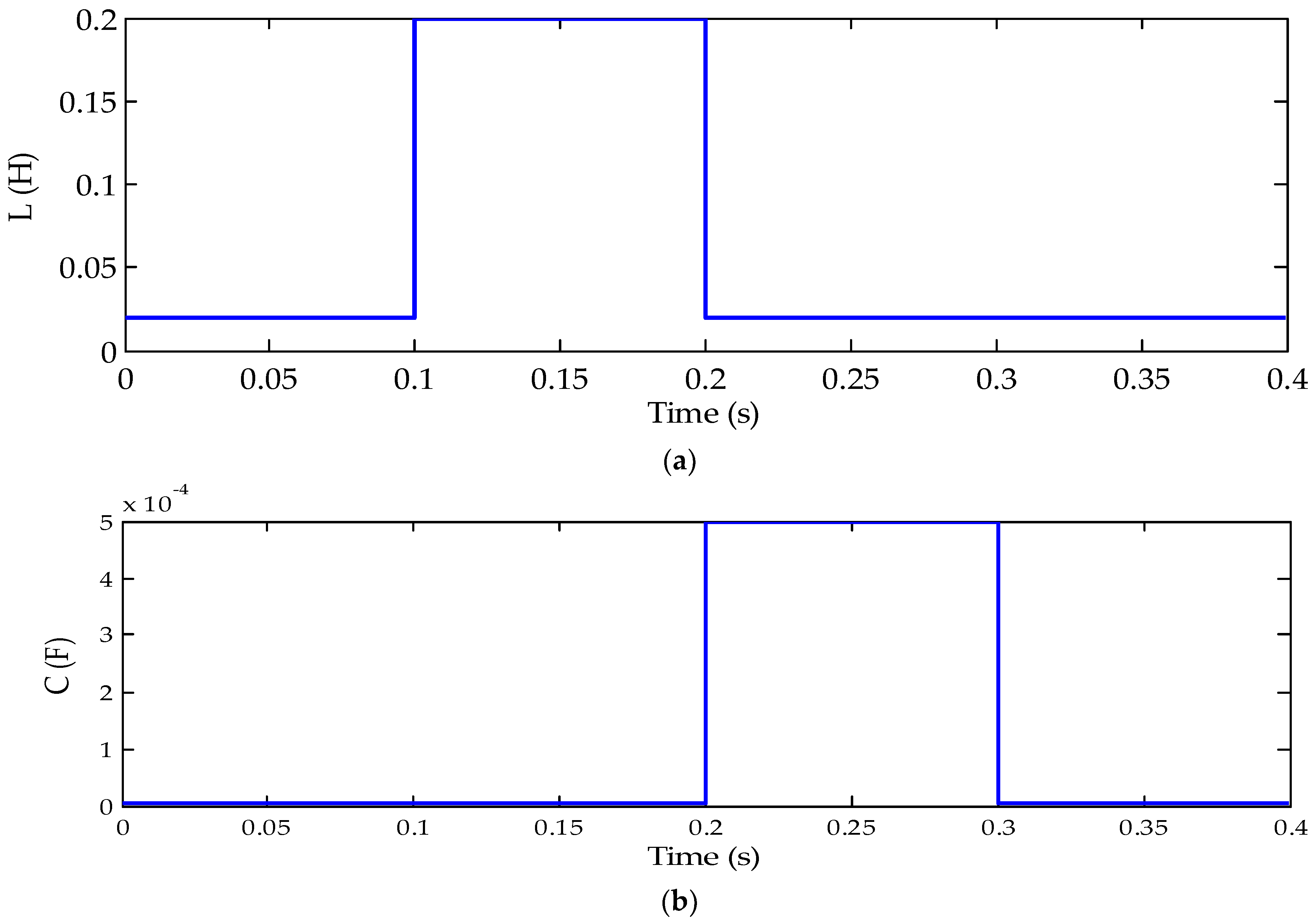
6.6. Controller’s Behavior under DC-DC Buck Converter Parameter Variations

As is well known, the PI and IP controllers are sensitive to system parameter variations. Thus, in this case, only the behavior of FLC, IMC, and the proposed SMC algorithms are tested. The DC input voltage, the load resistor, and the target output voltage are all held constant. Only the DC-DC buck converter parameter variations are considered in this case. Figure 12a,b show the adopted trajectories for the DC-DC buck converter inductor and capacitor, respectively. The obtained simulation results in this case are given in Figure 12c,d. The comparison performances of the three control algorithms in this case are summarized in Table 3.
It can be easily noted from both the obtained simulation results for different cases and the comparative study shown in Table 3 that the highest performance is achieved by the conceived SMC control algorithm, compared to the others.

7. Conclusions

In this paper, a mathematical model of the buck DC-DC converter is established. A robust control strategy is adopted for the output control voltage of the system. The validity of the latter is demonstrated using the Matlab/Simulink environment. In a comparative study with four control algorithms, PI, IP, FLC and IMC, the simulation results show that the designed sliding mode controller has robust characteristics and a fast dynamic response in the different studied cases.
Despite all these good performances, the chattering phenomenon remains the major problem of the used sliding mode control algorithm. To avoid this issue, we intend to use high-order sliding mode control for buck DC-DC converter control in future works.

Author Contributions

Supervision, M.B.H.; Validation, L.S.; Writing—review and editing, S.B.H. All authors have read and agreed to the published version of the manuscript.

Funding

This research received no external funding.

Institutional Review Board Statement

Not applicable.

Informed Consent Statement

Not applicable.

Data Availability Statement

Not applicable.

Conflicts of Interest

The authors declare no conflict of interest.

References

  1. Roncancio, J.S.; Vuelvas, J.; Patino, D.; Correa-Flórez, C.A. Flower greenhouse energy management to offer local flexibility markets. Energies 2022, 15, 4572. [Google Scholar] [CrossRef]
  2. Turoń, K.; Kubik, A.; Chen, F. What Car for Car-Sharing? Conventional Electric, Hybrid or Hydrogen Fleet? Analysis of the Vehicle Selection Criteria for Car-Sharing Systems. Energies 2022, 15, 4344. [Google Scholar] [CrossRef]
  3. Fady, M. Urban Freight Transport Electrification in Westbank, Palestine: Environmental and Economic Benefits. Energies 2022, 15, 4058. [Google Scholar]
  4. Sun, L.; Zhang, T.; Liu, S.; Wang, K.; Rogers, T.; Yao, L.; Zhao, P. Reducing energy consumption and pollution in the urban transportation sector: A review of policies and regulations in Beijing. J. Clean. Prod. 2021, 285, 125339. [Google Scholar] [CrossRef]
  5. Streltsov, A.; Malof, J.M.; Huang, B.; Bradbury, K. Estimating residential building energy consumption using overhead imagery. Appl. Energy 2020, 280, 116018. [Google Scholar] [CrossRef]
  6. Bandara, W.C.; Godaliyadda, G.M.R.I.; Ekanayake, M.P.B.; Ekanayake, J.B. Coordinated photovoltaic re-phasing: A novel method to maximize renewable energy integration in low voltage networks by mitigating network unbalances. Appl. Energy 2020, 285, 116022. [Google Scholar] [CrossRef]
  7. Guo, S.; Liu, Q.; Sun, J.; Jin, H. A review on the utilization of hybrid renewable energy. Renew. Sustain. Energy Rev. 2018, 91, 1121–1147. [Google Scholar] [CrossRef]
  8. Nie, P.; Roccotelli, M.; Fanti, M.P.; Ming, Z.; Li, Z. Prediction of home energy consumption based on gradient boosting regression tree. Energy Rep. 2021, 7, 1246–1255. [Google Scholar] [CrossRef]
  9. Mofidipour, E.; Babaelahi, M. New procedure in solar system dynamic simulation, thermodynamic analysis, and multi-objective optimization of a post-combustion carbon dioxide capture coal-fired power plant. Energy Convers. Manag. 2020, 224, 113321. [Google Scholar] [CrossRef]
  10. Aboagye, B.; Gyamfi, S.; Ofosu, E.A.; Djordjevic, S. Status of renewable energy resources for electricity supply in Ghana. Sci. Afr. 2020, 11, e00660. [Google Scholar] [CrossRef]
  11. IEA. World Energy Outlook 2015; OECD/IEA: Paris, France, 2015. [Google Scholar]
  12. NREL. Photovoltaic System Pricing Trends: Historical, Recent, and Near-Term Projections; National Renewable Energy Laboratory: Golden, CO, Canada, 2015. [Google Scholar]
  13. Panwar, N.L.; Kaushik, S.C.; Kothari, S. Role of renewable energy sources in environmental protection: A review. Renew. Sustain. Energy Rev. 2011, 15, 1513–1524. [Google Scholar] [CrossRef]
  14. Nassar, Y.F.; Abdunnabi, M.J.; Sbeta, M.N.; Hafez, A.A.; Amer, K.A.; Ahmed, A.Y.; Belgasim, B. Dynamic analysis and sizing optimization of a pumped hydroelectric storage-integrated hybrid PV/Wind system: A case study. Energy Convers. Manag. 2021, 229, 113744. [Google Scholar] [CrossRef]
  15. Leirpoll, M.E.; Næss, J.S.; Cavalett, O.; Dorber, M.; Hu, X.; Cherubini, F. Optimal combination of bioenergy and solar photovoltaic for renewable energy production on abandoned cropland. Sol. Energy 2021, 168, 45–56. [Google Scholar] [CrossRef]
  16. Tervo, E.J.; Callahan, W.A.; Toberer, E.S.; Steiner, M.A.; Ferguson, A.J. Solar thermoradiative-photovoltaic energy conversion. Cell Rep. Phys. Sci. 2020, 1, 100258. [Google Scholar] [CrossRef]
  17. Mellit, A.; Rezzouk, H.; Messai, A.; Mejahed, B. FPGA–based real time implementation of MPPT controller for photovoltaic systems. Renew. Energy 2011, 36, 1652–1661. [Google Scholar] [CrossRef]
  18. Houssamo, I.; Locment, F.; Sechilariu, M. Maximum power tracking for photovoltaic power system: Development and experimental comparison of two algorithms. Renew. Energy 2010, 35, 2381–2387. [Google Scholar] [CrossRef]
  19. Goudan, N.A.; Peter, S.A.; Nallandula, H.; Krithiga, S. Fuzzy logic controller with MPPT using line commutated inverter for three phase grid connected photovoltaic systems. Renew. Energy 2009, 34, 900–915. [Google Scholar]
  20. Ko, S.H.; Chao, R.M. Photovoltaic dynamic MPPT on a moving vehicle. Sol. Energy 2012, 86, 1750–1760. [Google Scholar] [CrossRef]
  21. Dawoud, S.M. Developing different hybrid renewable sources of residential loads as a reliable method to realize energy sustainability. Alex. Eng. J. 2021, 60, 2435–2445. [Google Scholar] [CrossRef]
  22. Debastiani, G.; Nogueira, C.E.C.; Acorci, J.M.; Silveira, V.F.; Siqueira, J.A.C.; Baron, L.C. Assessment of the energy efficiency of a hybrid wind-photovoltaic system for Cascavel. Renew. Sustain. Energy Rev. 2020, 131, 110013. [Google Scholar] [CrossRef]
  23. Loukil, K.; Abbes, H.; Abid, H.; Abid, M.; Toumi, A. Design and implementation of reconfigurable MPPT fuzzy controller for photovoltaic systems. Ain Shams Eng. J. 2019, 11, 319–328. [Google Scholar] [CrossRef]
  24. Padmanaban, S.; Priyadarshi, N.; Bhaskar, M.S.; Holm-Nielsen, J.B.; Hossain, E.; Azam, F. A hybrid photovoltaic fuel cell for grid integration with Jaya-based maximum power point tracking:experimental performance evaluation. IEEE Access 2019, 7, 82978–82990. [Google Scholar] [CrossRef]
  25. Priyadarshi, N.; Padmanaban, S.; Maroti, P.K.; Sharma, A. An extensive practical investigation of FPSO-based MPPT for grid integrated PV system under variable operating conditions with anti-islanding protection. IEEE Syst. J. 2019, 13, 1861–1871. [Google Scholar] [CrossRef] [Green Version]
  26. Shahid, H.; Kamran, M.; Mehmood, Z.; Saleem, M.Y.; Mudassar, M.; Haider, K. Implementation of the novel temperature controller and incremental conductance MPPT algorithm for indoor photovoltaic system. Sol. Energy 2018, 163, 235–242. [Google Scholar] [CrossRef]
  27. Bouchama, Z.; Khatir, A.; Benaggoune, S.; Harmas, M.N. Design and experimental validation of an intelligent controller for dc–dc buck converters. J. Frankl. Inst. 2020, 357, 10353–10366. [Google Scholar] [CrossRef]
  28. Batiyah, S.; Sharma, R.; Abdelwahed, S.; Alhosaini, W.; Aldosari, O. Predictive Control of PV/Battery System under Load and Environmental Uncertainty. Energies 2022, 15, 4100. [Google Scholar] [CrossRef]
  29. Chen, L.; Zheng, P.; Gao, W.; Jiang, J.; Chang, J.; Wu, R.; Ai, C. Frequency Modulation Control of Hydraulic Wind Turbines Based on Ocean Used Wind Turbines and Energy Storage. Energies 2022, 15, 4086. [Google Scholar] [CrossRef]
  30. Akram, N.; Khan, L.; Agha, S.; Hafeez, K. Global Maximum Power Point Tracking of Partially Shaded PV System Using Advanced Optimization Techniques. Energies 2022, 15, 4055. [Google Scholar] [CrossRef]
  31. Ge, Q.; Li, Z.; Sun, Z.; Xu, J.; Long, H.; Sun, T. Low Resistance Hot-Spot Diagnosis and Suppression of Photovoltaic Module Based on I-U Characteristic Analysis. Energies 2022, 15, 3950. [Google Scholar] [CrossRef]
  32. Olalla, C.; Rodriguez, M.; Clement, D.; Maksimovic, D. Architectures and Control of Sub module Integrated DC-DC Converters for Photovoltaic Applications. IEEE Trans. Power Electron. 2012, 28, 2980–2997. [Google Scholar] [CrossRef]
  33. Pilawa-Podgurski, R.C.N.; Perreault, D.J. Submodule integrated distributed maximum power point tracking for solar photovoltaic applications. IEEE Trans. Power Electron. 2013, 28, 2957–2967. [Google Scholar] [CrossRef] [Green Version]
  34. Carbone, R.; Borrello, C. Experimenting with a Battery-Based Mitigation Technique for Coping with Predictable Partial Shading. Energies 2022, 15, 4146. [Google Scholar] [CrossRef]
  35. Aluko, A.; Buraimoh, E.; Oni, O.E.; Davidson, I.E. Advanced Distributed Cooperative Secondary Control of Islanded DC Microgrids. Energies 2022, 15, 3988. [Google Scholar] [CrossRef]
  36. Guldemir, H. Study of sliding mode control of DC-DC buck converter. Energy Power Eng. 2011, 3, 401–406. [Google Scholar] [CrossRef] [Green Version]
  37. He, Y.; Luo, F.L. Study of sliding mode control for DC-DC converters. In Proceedings of the 2004 International Conference on Power System Technology, Singapore, 21–24 November 2004. [Google Scholar]
  38. Babes, B.; Boutaghane, A.; Hamouda, N.; Mezaache, M. Design of a Robust Voltage Controller for a DC-DC Buck Converter Using Fractional-Order Terminal Sliding Mode Control Strategy. In Proceedings of the 2019 International Conference on Advanced Electrical Engineering (ICAEE), Algiers, Algeria, 19–21 November 2019; pp. 1–6. [Google Scholar]
  39. Qamar, M.A.; Feng, J.; Rehman, A.U.; Raza, A. Discrete time sliding mode control of DC-DC buck converter. In Proceedings of the 2015 IEEE Conference on Systems, Process and Control (ICSPC), Sunway, Malaysia, 18–20 December 2015; pp. 91–95. [Google Scholar]
  40. Wang, Z.; Shihua, L.; Qi, L. Discrete-Time Fast Terminal Sliding ModeControl Design for DC–DC Buck Converters with Mismatched Disturbances. IEEE Trans. Ind. Inform. 2020, 16, 1204–1213. [Google Scholar] [CrossRef]
  41. Dehri, K.; Nouri, A.S. A discrete repetitive adaptive sliding mode control for DC-DC buck converter. Proc. Inst. Mech. Eng. I J. 2021, 235, 1698–1708. [Google Scholar] [CrossRef]
  42. Mobayen, S.; Bayat, F.; Lai, C.-C.; Taheri, A.; Fekih, A. Adaptive Global Sliding Mode Controller Design for Perturbed DC-DC Buck Converters. Energies 2021, 14, 1249. [Google Scholar] [CrossRef]
  43. Rakhtala, S.M.; Yasoubi, M.; Hosseinnia, H. Design of second order sliding mode and sliding mode algorithms: A practical insight to DC-DC buck converter. IEEE/CAA J. Autom. Sin. 2017, 4, 483–497. [Google Scholar] [CrossRef] [Green Version]
  44. Shi, S.; Xu, S.; Gu, J.; Min, H. Global High-Order Sliding Mode Controller Design Subject to Mismatched Terms: Application to Buck Converter. IEEE Trans. Circuits Syst. 2019, 66, 4840–4849. [Google Scholar] [CrossRef]
  45. Chi, X.; Lin, F.; Wang, Y. Disturbance and Uncertainty-Immune Onboard Charging Batteries With Fuel Cell by Using Equivalent Load Fuzzy Logic Estimation-Based Backstepping Sliding-Mode Control. IEEE Trans. Transp. Electrif. 2021, 7, 1249–1259. [Google Scholar] [CrossRef]
  46. Meng, Z.; Shao, W.; Tang, J.; Zhou, H. Sliding-Mode Control Based on Index control. Law for MPPT in Photovoltaic Systems. CES Trans. Electr. Mach. Syst. 2018, 2, 303–311. [Google Scholar] [CrossRef]
  47. Roy, T.K.; Faria, F.; Ghosh, S.K.; Pramanik, A.H. Robust Adaptive Backstepping Sliding Mode Controller for a DC-DC Buck Converter Fed DC Motor. In Proceedings of the 2021 Joint 10th International Conference on Informatics, Electronics & Vision (ICIEV) and 2021 5th International Conference on Imaging, Vision & Pattern Recognition (icIVPR), Virtual, 16–20 August 2021; pp. 1–6. [Google Scholar]
  48. Lim, S.; Kim, S.-K.; Kim, Y. Active Damping Injection Output Voltage Control with Dynamic Current Cut-Off Frequency for DC/DC Buck Converters. Energies 2021, 14, 6848. [Google Scholar] [CrossRef]
  49. Argyrou, M.C.; Marouchos, C.C.; Kalogirou, S.A.; Christodoulides, P. Modeling a residential grid-connected PV system with battery–super capacitor storage: Control design and stability analysis. Energy Rep. 2021, 7, 4988–5002. [Google Scholar]
  50. Abdelmalek, S.; Dali, A.; Bakdi, A.; Bettayeb, M. Design and experimental implementation of a new robust observer-based nonlinear controller for DC-DC buck converters. Energy 2020, 213, 118816. [Google Scholar] [CrossRef]
  51. Abedi, A.; Rezaie, B.; Khosravi, A.; Shahabi, M. DC-bus voltage control based on direct Lyapunov method for a converter based stand-alone DC micro-grid. Electr. Power Syst. Res. 2020, 187, 106451. [Google Scholar] [CrossRef]
  52. Ding, S.; Zheng, W.; Sun, J.; Wang, J. Second-Order Sliding-Mode Controller Design and Its Implementation for Buck Converters. IEEE Trans. Ind. Inform. 2018, 14, 1990–2000. [Google Scholar] [CrossRef]
  53. Derbeli, M.; Charaabi, A.; Barambones, O.; Sbita, L. Optimal Energy Control of a PEM Fuel Cell/Battery Storage System. In Proceedings of the 10th International Renewable Energy Congress (IREC), Sousse, Tunisia, 26–28 March 2019; pp. 1–5. [Google Scholar]
  54. Utkin, V. Variable structure systems with sliding modes. IEEE Trans. Autom. Control 1977, 22, 212–222. [Google Scholar] [CrossRef]
  55. Mihoub, M.; Nouri, A.S.; Ben Abdennour, R. Real-time application of discrete second order sliding mode control to a chemical reactor. Control Eng. Pract. 2009, 19, 1089–1095. [Google Scholar] [CrossRef]
  56. Utkin, V.I. Sliding Mode in Control and Optimization; Springer: Berlin/Heidelberg, Germany, 1992. [Google Scholar]
  57. Levant, A. Sliding order and sliding accuracy in sliding mode control. Int. J. Control 1993, 58, 1247–1263. [Google Scholar] [CrossRef]
  58. Sira-Ramirez, H. Structure at infinity, zero dynamics and normal forms ofsystems undergoing sliding motion. Int. J. Syst. Sci. 1988, 21, 665–674. [Google Scholar] [CrossRef]
  59. Sira-Ramirez, H. Non-linear discrete variable structure systems in quasi-sliding mode. Int. J. Control 1991, 54, 1171–1187. [Google Scholar] [CrossRef]
  60. Flah, A.; Sbita, L. A novel IMC controller based on bacterial foraging optimization algorithm applied to a high speed range PMSM drive. Appl. Intell. 2013, 38, 114–129. [Google Scholar] [CrossRef] [Green Version]
  61. Zadeh, L.A. Fuzzy sets. Inf. Technol. Control 1965, 8, 338–353. [Google Scholar] [CrossRef] [Green Version]
Figure 1. Synoptic scheme of the DC-DC buck converter.
Energies 15 06128 g001
Figure 2. Comparative study simulation results: (a) duty cycle, (b) control signal, (c) output voltages of DC-DC buck converter models and (d) model modeling error.
Energies 15 06128 g002aEnergies 15 06128 g002b
Figure 3. The internal model control of the feedback scheme.
Energies 15 06128 g003
Figure 4. Schematic of the fuzzy logic controller.
Energies 15 06128 g004
Figure 5. Fuzzy logic controller membership functions: (a) error membership function, (a) change error membership function and (b) evolution of target, and (c) change duty cycle membership function.
Energies 15 06128 g005
Figure 6. Closed loop control of buck control using sliding mode control approach.
Energies 15 06128 g006
Figure 7. Discontinuous function coefficient effect: (a) evolution of M coefficient, (b) evolution of the control voltage and (c) evolution of the output voltages.
Energies 15 06128 g007
Figure 8. Target output voltage variation: (a) evolution of the control voltage and (b) evolution of the output voltages.
Energies 15 06128 g008
Figure 9. Triangular target output voltage variation: (a) evolution of the control voltage and (b) evolution of the output voltages.
Energies 15 06128 g009aEnergies 15 06128 g009b
Figure 10. Input voltage variation: (a) evolution of the control voltage, (b) evolution of the control voltage and (c) evolution of the control voltage.
Energies 15 06128 g010aEnergies 15 06128 g010b
Figure 11. Resistor load variation: (a) evolution of the control voltage and (b) evolution of target and (c) actual output voltages.
Energies 15 06128 g011aEnergies 15 06128 g011b
Figure 12. DC-DC buck converter parameters variations: (a) trajectory of the inductor, (b) trajectory of capacitor, (c) control voltage and (d) output voltage.
Energies 15 06128 g012aEnergies 15 06128 g012b
Table 1. DC-DC buck converter parameters.
ParameterValue
Input voltage (v)400
Capacitor (µF) 5
Inductor (mH)20
Switching frequency (Khz) 10
Resistive load (Ω)10
Table 2. Rule-based table of the fuzzy logic controller.
C α ( k ) C e v ( k )
GNPNZPPGP
e v ( k ) GNGNGNPNPNZ
PNGNPNPNZPP
ZGN ZPPGP
PPPNZPPPPGP
GPZPPPPGPGP
Table 3. Comparative study between the five algorithms.
Control Algorithms
Operating ModesValuesParametersPIIPFLCIMCSMC
Abrupt target output variation150 vResponse time (ms)9.582.621.52.80.91
Tracking error (%)0.0130.0160.130.120.003
Overshoot (%) 00.2663.26 01.6
350 vResponse time (ms)8.52.62.52.82.6
Tracking error (%)2.8 × 10−32.9 × 10−41.2 × 10−31.4 × 10−37.1 × 10⁻⁵
Overshoot (%)4.480.171.170.0140.002
250 vResponse time (ms)1.47.89.22.10.7
Tracking error (%)0.330.010.040.020.001
Voltage loss (%) 00.110.44 00.8
Triangular target output variation20 × 103 v/sTracking error (v) 71.5157720−14.5
Abrupt input voltage variation400 vSettling time1.929.5813.42.81.3
Tracking error0.0250.040.10.1755 × 10−5
Overshoot 00.252 00.675
350 vStabilization time (ms)2.19.81.38 0
Tracking error (%)2 × 10−40.001 00.1 0
Voltage loss (%)2.256.658.33.550.001
300 vStabilization time (ms)182223.810.9 0
Tracking error0.040.01 00.1 0
Voltage loss (%)389.754.25 0
Abrupt load resistor variation15 ΩSettling time (ms)2.43.2413.63.70.89
Tracking error (%)0.11.0140.20.150.05
Overshoot (%) 0 00.450.11.7
10 ΩStabilization time (ms)3.26.828.770.8
Tracking error (%)0.150.120.130.055 × 10−5
Overshoot (%)7.2512.413.7510.2 0
Voltage loss (%) 1.1526.231.428.626.05
5 ΩSettling time (ms)2.49.9811.52.191.5
Tracking error (%)0.0010.0060.1250.025 0
Overshoot (%)7.112.1513.1510.45 0
Voltage loss (%)46.748.3548.646.846.45
Parameter
variations
Abrupt capacitor
variation
Stabilization time (ms)--13.713.9 0
Tracking error (%)--0.10.15 0
Overshoot/Voltage loss (%)--12.130 0
Abrupt inductor
variation
Stabilization time (ms)--0.110.12 0
Tracking error (%)--5 × 10−50.05 0
Overshoot/Voltage loss (%)--0.250.235 × 10−4
Number of controller tuning parameters0202030101
Publisher’s Note: MDPI stays neutral with regard to jurisdictional claims in published maps and institutional affiliations.

