Does Uncertainty Forecast Crude Oil Volatility before and during the COVID-19 Outbreak? Fresh Evidence Using Machine Learning Models

Abstract

This paper uses two competing machine learning models, namely the Support Vector Regression (SVR) and the eXtreme Gradient Boosting (XGBoost) against the Autoregressive Integrated Moving Average ARIMAX (p,d,q) model to identify their predictive performance of the crude oil volatility index before and during COVID-19. In terms of accuracy, forecasting results reveal that the SVR model dominates the XGBoost and ARIMAX models in predicting the crude oil volatility index before COVID-19. However, the XGBoost model provides more accurate predictions of the crude oil volatility index than the SVR and ARIMAX models during the pandemic. The inverse cumulative distribution of residuals suggests that both ML models produce good results in terms of convergence. Findings also indicate that there is a fast convergence to the optimal solution when using the XGBoost model. When analyzing the feature importance, the Shapley Additive Explanation Method reveals that the SVR performs significantly better than the XGBoost in terms of feature importance. During the pandemic, the predictive power of the CBOE Volatility Index and Economic Policy Uncertainty index for forecasting the crude oil volatility index is improved compared to the pre-COVID-19 period. These findings imply that investor fear-induced uncertainty in the financial market and economic policy uncertainty are the most significant features and hence represent substantial sources of uncertainty in the oil market.

1. Introduction

Oil has always been regarded as a significant comparative advantage for oil-producing countries. Indeed, oil is a primary source of revenue in oil-exporting countries, allowing them to accumulate more financial resources, particularly during periods of oil price spikes. The cartel of the world’s major oil-exporting countries, known as the Organization of Petroleum Exporting Countries (hereafter OPEC), was created in 1960 to coordinate and unify petroleum policies across its members (OPEC, 2021). According to the OPEC Annual Statistics Bulletin (2022), OPEC member countries accounted for 37.9% of world oil production and 80.4% of the proven oil reserves in 2021. OPEC is the main player determining oil supply and is consequently a major influencer of oil pricing on international markets. Crude oil prices are also important for policymakers in oil-importing countries, as oil is considered an input alongside capital and labor. A rise in oil prices induces a rise in transport and production costs, which may harm the well-being of people in those countries. Oil price upsurges may also have a detrimental impact on the public budget in countries with oil subsidies.

Over the past few decades, the oil market has experienced a wide range of events, making it one of the most volatile commodity markets [1,2,3].Events affecting the oil market may be political (Arab oil embargo in 1973–1974, the Iranian revolution in 1979, the Iraqi invasion of Kuwait in 1990, etc.) or economic (rise of production by OPEC members in 1986, rapid expansion of some emerging countries during the 1990s, occurrence of the 2007 Subprime crisis, etc.). Furthermore, the global health crisis due to the transmission of the COVID-19 pandemic has been associated with a drop in oil prices because of lockdown measures and the fall in the global oil demand [4,5].

The post-global financial crisis literature on the drivers of crude oil volatility has grown remarkably. Many researchers, such as [6,7,8], argued that it is essential to address this issue because of the high risk that small changes in crude oil prices will damage national economies and energy markets. Furthermore, Jo [9] asserted that crude oil volatility plays a substantial role in heightening uncertainty about the stability of the energy market in the short to medium term. The author further added that the authorities are forced to bear additional energy costs, which increases the budget burden. Furthermore, as the COVID-19 pandemic spread worldwide in 2020, the debate over the risks of oil price volatility has revived, particularly since the pandemic has impacted the global economy. The oil market saw a dramatic plunge in oil futures prices as the health crisis worsened and lockdown measures were enacted, reaching sub-zero levels on 20 April 2020. This was mainly due to inexperienced traders holding on to the May contracts until the end of the latest session before the settlement date. Traders failed to offload these contracts and sell them to oil refineries, which refrained from buying in light of the market shock, only to find themselves forced to receive crude oil with storage difficulties. Assaf et al. [10] further asserted that the volatility of crude oil prices during the COVID-19 outbreak increased investors’ uncertainty about the profitability of their investments in risky assets, such as crude oil. This shift in price fluctuations during the pandemic has been well reflected by the increase in the fear index, as represented by the CBOE crude oil volatility index. Such index increased from 25.16 percentage points on 27 December 2019, to 173.53 percentage points on 24 April 2020.

A growing body of knowledge has recently focused on factors affecting crude oil price fluctuations during the COVID-19 pandemic [10,11]. According to Wu et al. [8], studying oil price fluctuations is important for investors and policymakers. An effective assessment of crude oil price fluctuations and their fundamentals enables policymakers to implement appropriate measures and hedging policies and enables investors to manage their risky portfolios optimally during the health crisis. For example, Bourghelle et al. [12] analyzed the impact of crude oil supply and demand shocks on oil price volatility during the COVID-19 outbreak. The authors concluded that there was significant uncertainty induced by the two shocks and therefore increased crude oil volatility. Additionally, Christopoulos et al. [13] examined the response of crude oil volatility to COVID-19 infections and deaths in six geographic areas. It has been shown that the pandemic represented a significant risk to the economy, as the results suggest an increase in uncertainty accompanied by an increase in crude oil fluctuations. The authors concluded that asset managers and investors should incorporate the pandemic as an important factor in their short- and medium-term decisions. Moreover, Echaust and Just [11] explored the effect of OVX index variations on crude oil returns using a static and dynamic conditional copula procedure. The study reveals a significant impact of OVX index variations on crude oil returns during the COVID-19 pandemic. Similarly, Assaf et al. [10] investigated the prominent role of trade, stock market, economic policy, and geopolitical risk uncertainty on the energy market. The authors analyzed the spillover effect of various uncertainty indices on crude oil returns from January 2020 to July 2020. The time-varying parameter vector autoregressive-based connectedness approach reveals that economic policy uncertainty and global trade uncertainty are the most important sources of energy market fluctuations during the pandemic.

Unlike previous studies, the present paper aims to forecast the CBOE crude oil volatility index using information contained in several uncertainty measures related to financial markets (CBOE Volatility Index, VIX; Infectious Disease Tracking Index, IDEMV), economic policy conditions (Economic Policy Uncertainty Index, EPU; Geopolitical Risk Index, GPR). For this purpose, we particularly employ the eXtreme Gradient Boosting (XGBoost) machine learning method on a daily dataset. This method was recently developed by Chen and Guestrin [14]. There are several motivations for implementing this new machine learning tool. (a) XGBoost is characterized by its advanced learning speed and performance ability. Jabeur et al. [15] reported that XGBoost is robust in providing good and correct predictions and reducing data complexity; (b) uncertainty in energy markets represents an important source of complex features in the data, including non-stationarity, nonlinearity, skewness, and time-varying structure. In the presence of these complex features, standard methods of forecasting energy prices become inappropriate [7]. Indeed, Ftiti et al. [7] and Wu et al. [16] emphasized the importance of using machine learning tools to forecast energy prices accurately. In this respect, the XGBoost model allows considering the abovementioned data characteristics, as it is robust to complexity; (c) the XGBoost computational method can examine the simultaneous effect of several inputs at the same time. This is due to its fast process and higher accuracy with lower complexity and cost. This allows the combination of various inputs to generate an improvement in forecasting accuracy, together with applying the Shapley Additive explanation (SHAP) to detect the importance of specific features of energy variables. It is worth noting that the performance of the XGBoost machine learning model is compared to a second machine learning model, i.e., the Support Vector Regression (SVR) and a standard forecasting model, i.e., the Autoregressive Integrated Moving Average (ARIMAX (p,d,q)).

This paper makes several important contributions to recent literature. First, previous studies concluded that uncertainty measures have significant explanatory power for crude oil fluctuations during the pandemic. However, this is still insufficient to achieve the short- and medium-term equilibrium in the energy market, as there are no prior studies that focused on analyzing investors’ concerns about oil price fluctuations. This study is the first to examine the mutual impact of several uncertainty indicators on the crude oil volatility index. To the best of our knowledge, no study investigated the co-effects of various uncertainty indices on the crude oil volatility index during the COVID-19 outbreak. Second, the complex interactions between implied volatility (VIX), economic policy uncertainty (EPU), the infectious disease EMV tracker (IDEMV), and geopolitical risk (GPR) prompt us to employ the nonlinear XGBoost method. This paper is the first to implement the XGBoost machine learning to forecast crude oil volatility. Third, the importance of oil for both oil-exporting and oil-importing countries and the recurrence of sharp oil price volatility over the last decades make the forecasting of oil prices a priority for both investors and policymakers. Indeed, accurate oil price forecasts allow investors to decide on the structure of their portfolios and policymakers to manage public deficits better. The results of this study will also have important implications for policymakers and energy traders. They will enable them to identify the nature of the association between investments in oil futures and the crude oil volatility index, as well as the impact of this relationship on energy market stability.

The rest of this paper is organized as follows. The literature review is presented in Section 2. Section 3 describes the data and the methodological framework. Section 4 is reserved for the discussion of results. A robustness analysis is conducted in Section 5. In Section 6, we draw the main concluding remarks and policy implications.

2. Related Literature

Since the seminal work of Hamilton [17], there has been a proliferation of studies on factors affecting crude oil volatility. The common objective of prior studies has always been to accomplish accurate modeling and forecasting of oil price volatility. The first group of studies considered macroeconomic variables, such as oil shocks, oil supply, gas prices, oil demand, and the economic activity [7,18,19,20,21].

The second group of studies rather focused on financial, speculative and social media factors, such as the exchange rate, the interest rate, the stock market, the trading volume ratio of oil futures, the sentiment analysis and social media information [8,22,23,24,25,26,27,28]. For example, Orzeszko [28] performed the nonlinear Granger causality tests to test the nonlinear causal relationship between oil price and exchange rate. The results support a strong bidirectional causal relation between crude oil prices and two currency pairs: EUR/USD, GBP/USD, and weaker between crude oil prices and JPY/USD. The Support Vector Regression (SVR) was applied to forecast this relationship. Findings indicate that the SVR models do not outperform the benchmark white noise model. In addition, Wu et al. [8] used oil price, oil production, oil consumption, and oil inventory to forecast the U.S. oil markets based on social media information during the COVID-19 pandemic. Results indicate that social media information is determinant in forecasting oil price, oil production and oil consumption. Hence, to forecast oil prices, marketers must consider the impact of social media information, especially during the COVID-19 pandemic. Using Web-based Sentiment Analysis, Zhao et al. [27] aimed to forecast oil prices. Findings indicate that the different types of sentiments can all improve performance but by similar amounts. The authors also report that text with strong intensity can better support oil price forecasting than weaker text.

A growing literature has emerged in recent years on the role of uncertainty. For example, Dutta et al. [29] highlighted the importance of addressing crude oil price uncertainty due to its potential impact on economic stability and financial markets. Seen in this light, the most important indicator of uncertainty is the policy uncertainty index. Since the pioneering study of Baker et al. [30], the EPU has been widely used for explaining and predicting crude oil volatility. Bekiros et al. [31] employed different vector autoregressive models to examine the linkages between EPU and WTI oil prices from January 2007 to February 2014. The results suggest that the information contained in the EPU index has a significant prediction power to explain WTI oil price fluctuations. Using daily and monthly data and the GARCH-MIDAS model, Wei et al. [32] concluded that the EPU index could predict the volatility of WTI crude oil price fluctuations. Similarly, Ma et al. [33] used the GARCH-MIDAS model and data spanning from 1 January 1998 to 31 May 2018. The results confirm that the EPU could predict the volatility of crude oil in the long run. Bakas and Triantafyllou [34] examined the effect of EPU on crude oil volatility. The empirical findings of volatility models performed on monthly data reveal that economic policy uncertainty could predict crude oil volatility. In addition, Yang [35] explored the interaction between the EPU and WTI and BRENT crude oil prices. The structural vector autoregressive model provides a significant correlation between EPU and crude oil prices. Using wavelet coherence modeling, Qin et al. [36] investigated the linkages between WTI oil prices and the EPU from January 1986 to August 2019. The analysis shows that changes in the US uncertainty affect WTI oil price. Similarly, Li et al. [26] examined the effects of two economic uncertainty measures, the global economic policy uncertainty, and the US economic policy uncertainty. The application of the extended GARCH-MIDAS models leads to the conclusion that the two policy uncertainty indices provide accurate forecasts of crude oil volatility in the in-sample analysis. The out-of-sample analysis, however, suggests that the US economic policy uncertainty dominates the global economic policy uncertainty in forecasting crude oil volatility.

Alongside the literature on policy uncertainty, another body of research has investigated the effectiveness of geopolitical risk in predicting the crude oil prices volatility. To illustrate, Liu et al. [37] examined the WTI and GPR linkages based on daily and monthly data from January 1986 to May 2017. Through the application of the GARCH-MIDAS model, they reported that the geopolitical risk index predicts the volatility of oil prices. Similarly, Liu et al. [37] and Li et al. [26] implemented the GARCH-MIDAS model on daily data from 2 January 1997 to 31 July 2017. The authors reveal that the GPR index significantly predicts crude oil volatility. Based on the MIDAS model, Mei et al. [38] concluded that the GPR index positively affected the realized volatility of crude oil between 1 January 2007, and 15 July 2016. Tiwari et al. [39] estimated the effect of the GPR index on the crude oil price volatility from 2 January 1985 to 30 November 2017, using the Markov-Switching time-varying copula model. The authors reported that the GPR index negatively affects the relationship between crude oil and gold. Recently, Nonejad [40] employed a simple predictive framework on daily data and confirmed that the GPR index predicts crude oil price volatility.

Another strand of the literature has investigated the predictive power of the implied volatility index on crude oil volatility. For example, Bakas and Triantafyllou [34] estimated the effects of the implied volatility index on monthly crude oil price volatility. The empirical results indicate that the implied volatility predicts crude oil volatility. Recently, Dutta et al. [29] investigated the predictive power of the implied volatility index for crude oil volatility. The authors confirmed the existence of a significant effect of implied volatility on crude oil volatility. Recently, Lu et al. [41] used the Markov regime-switching method to examine the effect of the COBE implied volatility index on the oil futures market. The authors concluded that the implied volatility has a significant impact on the oil market. It is worth noting that few studies investigated the impact of the newspaper-based infectious disease EMV tracker index on the crude oil price. For instance, using the heterogeneous autoregressive realized volatility model, Bouri et al. [42] revealed that the market uncertainty generated by infectious diseases predicts the oil market volatility.

Based on the above review, one may mention that the previous literature remains somewhat silent regarding the potential predictive power of the different uncertainty measures for crude oil price volatility. In this paper, we enrich the existing knowledge by exploring the role of machine learning techniques in predicting the crude oil volatility index using different uncertainty indices.

3. Data and Methodology

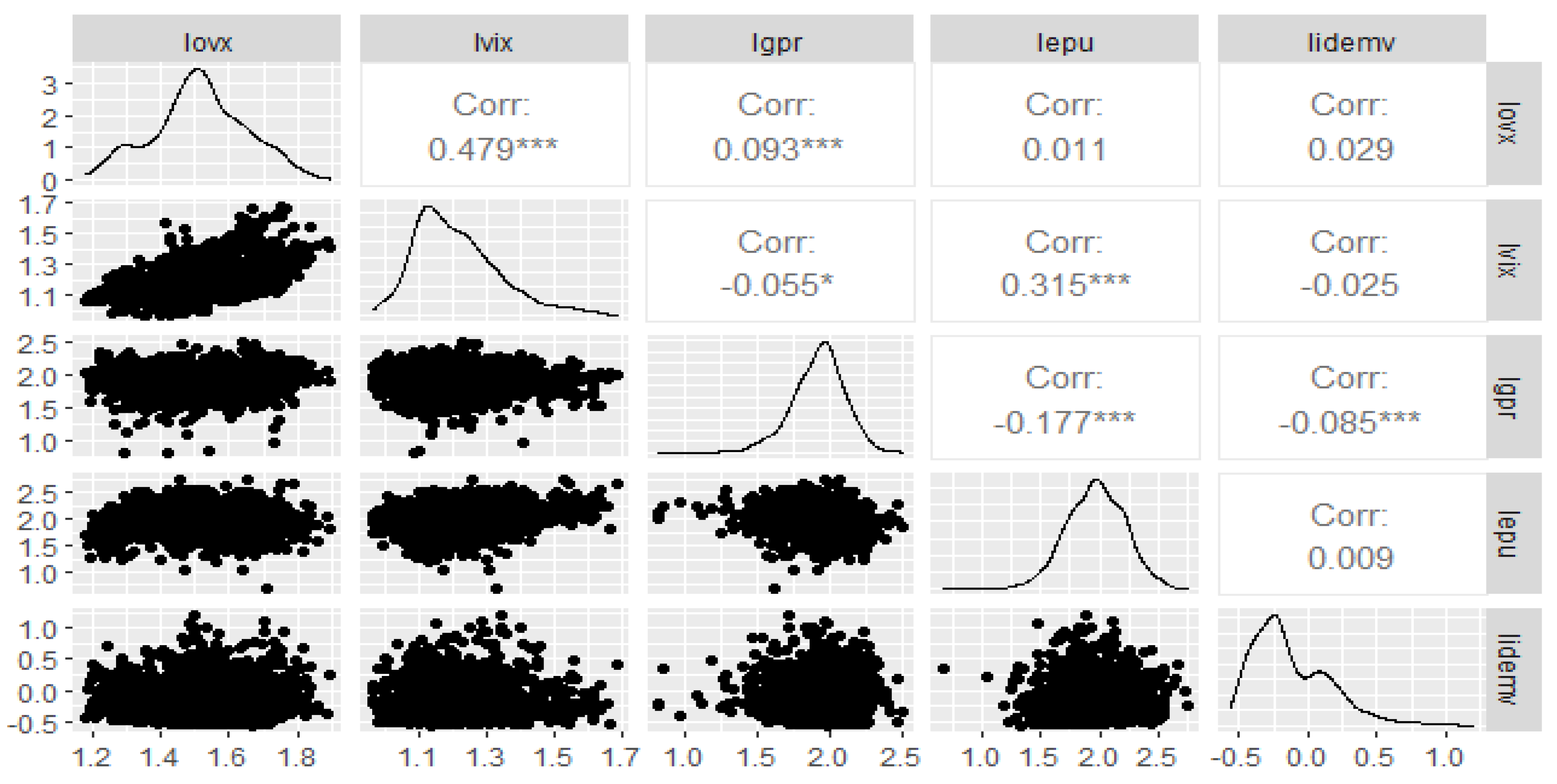
3.1. Data Analysis

The data includes daily values of the Crude Oil Volatility Index (OVX), US Economic Policy Uncertainty Index (EPU), Chicago Board Options Exchange Volatility Index (VIX), Geopolitical Risk Index (GPR), and Daily Infectious Disease Equity Market Volatility Tracker (IDEMV). The EPU, GPR, and IDEMV are obtained from https://www.policyuncertainty.com/ (accessed on 1 October 2021). The EPU index indicates the number of newspaper articles dealing with financial regulation, economic, monetary, and trade policy uncertainty in the United States. The GPR index represents the total number of newspaper articles covering geopolitical events and tensions. Finally, the IDEMV index is defined as the total number of newspaper articles covering terms related to infectious diseases (epidemic, disease, coronavirus...), equities (financial economy...), markets (Standard and Poors, stock market...), and volatility (volatility, risk, uncertainty...). The VIX and OVX indices are collected from the CBOE website (The unit of these variables is the percentage point). Whaley [43] was the pioneer in inventing the VIX to measure uncertainty in financial trading. Tissaoui [44] illustrated that the VIX represents investors’ sense of fear in the market. Similarly, the Chicago Board Options Exchange also created the OVX to represent the fear sentiment in the oil market.

The study is based on daily data and covers a relatively long period from 1 January 2010 to 31 August 2021. The full period is divided into two sub-periods, before and after 31 December 2019, when the World Health Organization’s China country office was officially informed of cases of pneumonia in Wuhan City. In other words, the first period runs from 1 January 2010 to 30 December 2019. We choose this period 2010–2020 given the stability of the OVX index during this period. As a matter of fact, we noticed that this index was high during the financial crisis of 2008/2009, since it was estimated at 93.05 percentage points on 12 December 2008, then it was stable during the period from 2010 to 2019, before experiencing a significant increase during the month of March 2020, estimated at around 190.08 percentage points.

A total of 3286 observations are preserved for training the model during this period, while 365 observations are devoted to the validation stage. The second period represents the COVID-19 outbreak starting on 31 December 2019, to 31 August 2021. The training stage is done using 488 observations, while 122 observations are kept for the validation stage. By doing so, the empirical analysis is conducted before and during the COVID-19 and allows comparing the predictive power of the set of uncertainty indexes in forecasting the crude oil price volatility index in normal and health crisis periods.

Table 1. Descriptive statistics.

	Mean	Median	Max	Min	Std. Dev.	Skewness	Kurtosis	J-B	Obs.
Panel A. Pre-COVID-19
OVX	33.14	31.69	78.97	14.50	10.20	0.87	3.99	614.0960	3651
VIX	16.81	15.43	48.00	9.14	5.65	1.76	6.92	4208.202	3651
EPU	109.72	94.77	586.55	3.32	63.83	1.65	7.76	5105.250	3651
GPR	93.50	88.36	361.02	6.69	39.26	1.10	5.48	1677.320	3651
IDEMV	0.43	0.00	15.91	0.00	0.90	6.17	65.71	621,436.5	3651
Panel B. COVID-19
OVX	53.38	40.15	325.15	27.66	35.86	3.07	14.06	4065.344	610
VIX	25.22	22.72	82.69	12.10	10.68	2.15	9.12	1424.659	610
EPU	240.53	195.95	861.10	20.63	152.31	1.19	4.13	176.4942	610
GPR	79.54	72.75	420.29	3.73	42.54	2.18	15.01	4148.166	610
IDEMV	19.61	16.43	112.93	0.00	14.87	1.83	8.53	1115.84	610

Note: Table 1 reports the descriptive statistics, including the mean, median, standard deviation (std. dev.), skewness, kurtosis, minimum (min), maximum (max) Jarque-Bera (J-B) and the number of observations (obs.), of the daily innovations of OVX, VIX, EPU, GPR, and IDEMV before and during the COVID-19 outbreak.

reports some descriptive statistics of the data.

Values of the Jarque–Bera test are significant at 1%. Furthermore, all series are characterized by an upper non-normal distribution before and during the crisis. In addition, the skewness values are positive and above zero for all variables, confirming the existence of asymmetric behavior in the data. Furthermore, all kurtosis values are greater than 3, which means that variables have heavier tails than a normal distribution. Figure 1 and Figure 2 show the correlation matrix between all variables.

The results indicate that the OVX index has a positive and moderate correlation with VIX before the pandemic. However, it has a positive and weak correlation with EPU, GPR, and IDEMV. During COVID-19, the figures indicate that the correlations of OVX with VIX, EPU, and IDEMV improved. The correlation coefficients are positive and relatively high. Regarding the connections between OVX and GPR, the matrix reveals that the correlation is negative and low.

3.2. Methodology

Machine learning (ML) refers to the capacity of computers to start learning from a particular training dataset and then continue to apply it to a new dataset. Hao et al. [45] suggested that machine learning may potentially detect the nonlinear hidden pattern and non-stationarity in the series. Similarly, many authors concluded that machine learning is the most popular time series forecasting method [26]. Another justification for their popularity is that these methods are more relevant for continuous variables, such as crude oil prices.

In the present study, we explore the performance of two competing machine learning methods for forecasting the crude oil volatility index: Support Vector Regression and eXtreme Gradient Boosting. However, to identify the values of the fitting parameters from SVR and XGBoost methods, a resampling approach is used to evaluate the performance of the model on the training set. There are different resampling methods, with k-fold cross-validation being one of the more common types. The process is repeated several times, and the performance estimates from each expectation set are averaged into a final overall estimate of the model’s effectiveness so that, given the training set, the algorithm generates a prediction function $f$. For each combination of parameters, the model fit is estimated by resampling, and the relationship between the fit parameters and the model performance is evaluated.

3.2.1. Support Vector Machine (SVM)

The Support Vector Machine was developed by Vapnik [46] as a supervised classification method which may also be used in regression using the structural risk minimization (SRM) approach for classification and regression. The SVM method assumes that for a training data ${\left\{x_{i }, y_i\right\}}_{i=1}^n$ where $x_{i }\in R^L$ is a vector of $L$ input features, $y_{i }\in R^L$ the output target, and ($n$) is the total number of data models.

The objective of SVM is to find a function $f\left(x\right)$ that predicts the output value whose deviation from the desired output $y_{i }$ is smaller than the insensitive loss parameter ($\epsilon$) for all training data, and at the same time, it is as flat as possible [47].The regression function that is linear in the low-dimensional space is described mathematically as follows:

$$f\left(x\right)=w{x}_i+b$$

(1)

where $x$ is the vector of weights which is normal to the hyperplane, and $b$ is the bias of the hyperplane. The regression problem is converted to an optimization problem as follows:

$$\begin{gathered} \mathit{minimize} \frac{1}{2}\parallel {\omega }^2\parallel +C{\sum }_{i=1}^n({\xi }_i+{\xi }_i^{\ast }) \\ \mathit{subjected}\mathit{to} \{\begin{array}{c}{y}_i-\langle \omega \left(x_i\right)\rangle -b\le \epsilon +{\xi }_i\\ \langle \omega \left(x_i\right)\rangle +b-y_i\le \epsilon +{\xi }_i^{\ast }\\ {\xi }_i,{\xi }_i^{\ast }\ge 0\end{array} \end{gathered}$$

(2)

where ${\xi }_i,{\xi }_i^{\ast } \in R$ are the flexible variables, and $C$ is the coefficient of penalty. The Lagrange multiplier is entered to overcome the optimization problem, and the regression function becomes as follows:

$$\begin{gathered} f(x)=\sum _{i=1}^{n_{sv}}({\alpha }_i-{\alpha }_i^{\prime })k(x_i,x_i^{\prime })+b \\ \mathrm{Subject} \mathrm{to} 0\le {\alpha }_i^{\prime }\le C, 0\le {\alpha }_i\le C \end{gathered}$$

(3)

where ${\alpha }_i,{\alpha }_i^{\prime }$ represents the Lagrange multiplier, $n_{sv}$ denotes the number of Support Vector, $k\left(x_i,x_i^{\prime }\right)$ is the kernel function. The Karush Kuhn-Tucker (KKT) conditions are employed to determine b [47,48].

3.2.2. eXtreme Gradient Boosting (XGBoost)

The XGBoost method is a machine learning technique developed by Ostrowski and Birman [49]. It can be applied for both regression and classification problems. Moreover, it has been adopted in various domains, such as healthcare [50] and the metal market [15]. Based on the gradient direction of their loss function, a weak learner is generated at each step and accumulated in the total model. In addition, the output function is normalized to eliminate over-fitting and speed up the learning process. The output function of the model is defined as:

$${\widehat{Y}}_i^T={\displaystyle \sum }_{k=1}^T{f}_k\left(x_i\right)={\widehat{y}}_i^{T-1}+f_T\left(x_i\right)$$

(4)

where ${\widehat{y}}_i^{T-1}$ denotes the generated tree, $f_T\left(x_i\right)$ represents the new tree model, and $T$ refers to the entire number of tree models. The following objective function is minimalized:

$$ℒ(\varphi )=\sum _{i}l(y_i,{\hat{y}}_i)+\sum _k\Omega (f_T)$$

(5)

where $ℒ$ is the loss function. In order to prevent too large complexity of the model, the penalty term $\Omega$ is included as follows:

$$\Omega \left(f_T\right)=\gamma N+\frac{1}{2}\lambda \parallel w{\parallel }^2$$

(6)

where $\gamma$ and $\lambda$ are parameters controlling penalty for the number of leaves N and magnitude of leaf weights $w$, respectively. The purpose of $\Omega \left(f_T\right)$ is to prevent over-fitting and to simplify models produced by this algorithm.

Ma et al. [51] pointed out that XGBoost is robust in terms of modeling nonlinear associations between variables. It has a high classification capability. Similarly, many scholars emphasized that machine learning is a powerful technique for predicting time series. However, it does not provide interpretable inference like traditional econometrics. In order to improve the performance of XGBoost, Lundberg and Lee [52] proposed a Shapley Additive Explanation Method (SHAP) to make predictive interpretations of ML techniques based on the game theory advanced by Shapley [53].When using the SHAP approach, we could understand the prediction of a specific input ($X$) by calculating the impact of each feature on the prediction. The main idea of SHAP is to calculate Shapley values for each feature of the sample to be analyzed, where each Shapley value is representative of the impact of the feature with which it is associated with the prediction. In addition, ML models usually have a very large number of features, with each feature being a discrete or continuous variable, making the calculation of Shapley values for each feature instance quite complicated. The SHAP method is therefore appropriate to address our research problem.

The estimated Shapley value is calculated as follows:

$${\widehat{\varphi }}_j=\frac{1}{K}{\displaystyle \sum }_{k=1}^K\left(\widehat{g}\left(x_{+j}^m\right)-\widehat{g}\left(x_{-j}^m\right)\right)$$

(7)

where; $\widehat{g}\left(x_{+j}^m\right)$ is the prediction for $x$, but with a random number of feature values.

3.2.3. Autoregressive Integrated Moving Average ARIMAX (p,d,q) Models

In the present study, we consider ARIMAX (p,d,q) as the traditional model. The reason for using this model is its ability to capture the long memory behaviour shown in the uncertainty indices. The ARIMAX (p,d,q) model is described as follows:

$$\begin{array}{cc}{\Delta }^d{\mathrm{OVX}}_t=& \delta +{\sum }_{i=1}^p{\phi }_{i}OV{X}_{t-i}+{\sum }_{i=1}^k{\omega }_{i}VI{X}_{t-i}+{\sum }_{i=1}^k{\alpha }_{i}EP{U}_{t-i}+{\sum }_{i=1}^k{\beta }_{i}GP{R}_{t-i}+\hfill \\ & {\sum }_{i=1}^k{\gamma }_i\mathit{IDEM}{V}_{t-i}+{\sum }_{i=0}^q{\sigma }_i{\epsilon }_{t-i}.\hfill \end{array}$$

(8)

where ${\mathrm{OVX}}_t$ is the crude oil volatility; $OV{X}_{t-i}$ are the previous values of the OVX; $VI{X}_{t-i}$, $EP{U}_{t-i}$, $GP{R}_{t-i}$ and $IDEM{V}_{t-i}$ are the preceding values of the VIX, EPU, GPR, and IDEMV, respectively. δ is a constant, and d denotes the order of integration. ${\omega }_i$, ${\phi }_i$, ${\alpha }_i, {\beta }_i, {\gamma }_i$ and ${\sigma }_i$ represent the coefficients, and k, p, and q are the maximum time lags of the forecasters’ sequences, output sequence, and residuals, respectively. The determination of ARIMAX (p,d,q) is performed by the method of Box and Jenkins. Afterwards, in order to select the best model among several ARIMAX (p,d,q) models, the Akaike Information Criterion (AIC) is applied.

3.2.4. The Performance Metrics

The forecast performance is evaluated using three criteria: the Root Mean Square Error (RMSE), the Mean Squared Error (MSE), and the coefficient of determination ($R^2$) [54]. To calculate the performance metrics, we use the following formulas:

$$\mathrm{MSE}=\frac{1}{N_v}{{\displaystyle \sum }}_{t=1}^{N_v}\left(y_t-\widehat{y_t}\right)$$

(9)

$$\mathrm{RMSE}=\sqrt{\frac{1}{N_V}{\displaystyle \sum }_{t=1}^{N_V}{\left(y_t-{\widehat{y}}_t\right)}^2}$$

(10)

$$R^2=1-\frac{\frac{1}{N_V}{{\displaystyle \sum }}_{t=1}^{N_V}{\left(y_t-{\widehat{y}}_t\right)}^2}{\frac{1}{N_V}{{\displaystyle \sum }}_{t=1}^{N_V}{\left(y_t-\overline{y}\right)}^2}$$

(11)

where ${\widehat{y}}_t$ represents the forecasted crude oil volatility index,$y_t$ is the t-th actual crude oil volatility index, $\overline{y}$ is the mean of the crude oil volatility index, and $N_v$ is the number of observations used during the validation stage.

4. Empirical Results

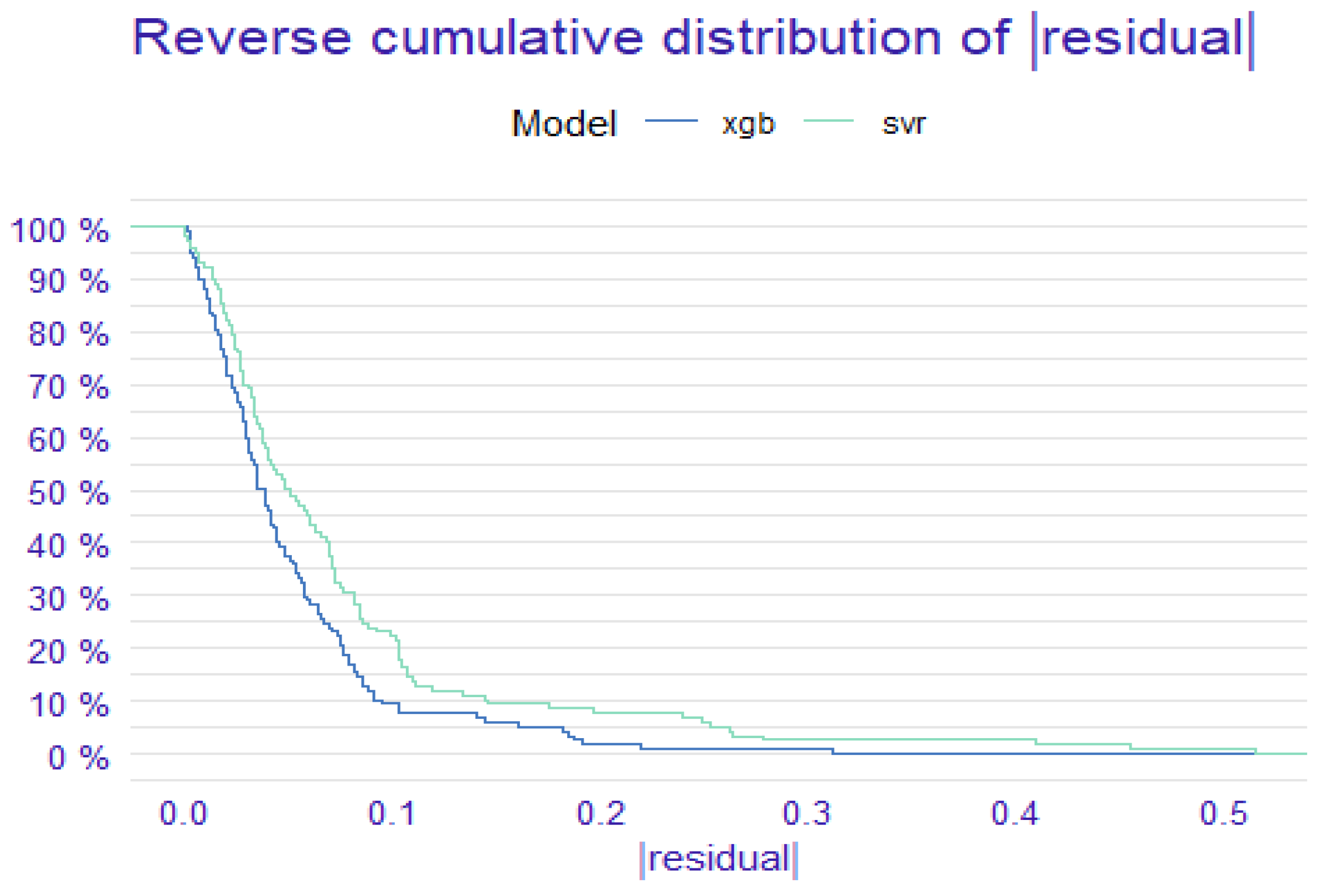
4.1. Forecasting Analysis

Implementing the Support Vector Machine and eXtreme Gradient Boosting methods to forecast crude oil volatility index provides important findings. The process involves studying the simultaneous effect of VIX, EPU, GPR, and IDEMV on the OVX. Figure 3 shows the predicted and actual OVX series before the COVID-19 outbreak. The figure shows that curves of the predicted values using the SVM and XGBoost models have almost the same pattern as the actual values of the crude oil volatility index at the beginning and end of the validation sample. Nevertheless, the curves generated by the two machine learning models are different from the curve of the actual values during the middle of the validation sample.

Overall, the figure indicates that the two methods provide accurate forecasts of the crude oil volatility index across most of the validation samples. However, using only Figure 3 to determine the best-fit model is insufficient. To provide more details, we report in

Table 2. Prediction performance assessment of the candidate models (Daily analysis).

Pre-COVID-19				COVID-19
Models	RMSE	MSE	${\mathit{R}}^2$	RMSE	MSE	${\mathit{R}}^2$
XGBoost	0.120	0.014	0.210	0.070	0.005	0.840
SVM	0.112	0.013	0.260	0.100	0.012	0.710
ARIMAX	0.149	0.022	0.320	0.151	0.023	0.319

some performance metrics: the RMSE, MSE, and $R^2$. As shown, the SVM model dominates the XGBoost model in predicting OVX. Indeed, the results suggest that the performance metrics of the SVM model (RMSE = 0.112; MSE = 0.013) are lower than those of the XGBoost model (RMSE = 0.12; MSE = 0.014). Similar conclusions are reached when considering the coefficient of determination $R^2$ which equals 0.26 for SVM and 0.21 for XGBoost. However, given the low performance results, the ARIMAX model is eliminated while the XGBoost and SVR models are retained.

Figure 4 shows that the two ML models perform quite well in predicting the crude oil volatility index during COVID-1. Moreover, the XGBoost model predicts the OVX with high accuracy, as it almost makes the red line (actual OVX) and the blue line match up (predicted OVX) over the pandemic period, especially in the latter part of the forecast sample. Similarly, the SVM model performed well with some differences. We find that the predicted value curve (green line) and the actual value curve of the OVX (red line) have almost the same pattern. However, it is less pronounced than that of the XGBoost model. These findings indicate that the predictive accuracy of the XGBoost model has been improved. Furthermore, the performance measures reported in Table 2 support these results. We found that the XGBoost tool imposes its dominance over the SVM model, as it produces the lowest error value for RMSE (0.07) and MSE (0.005) and the highest value for $R^2$ (0.84). This means that the nonlinear XGBoost model performs better than the linear SVM model in predicting OVX during COVID-19.

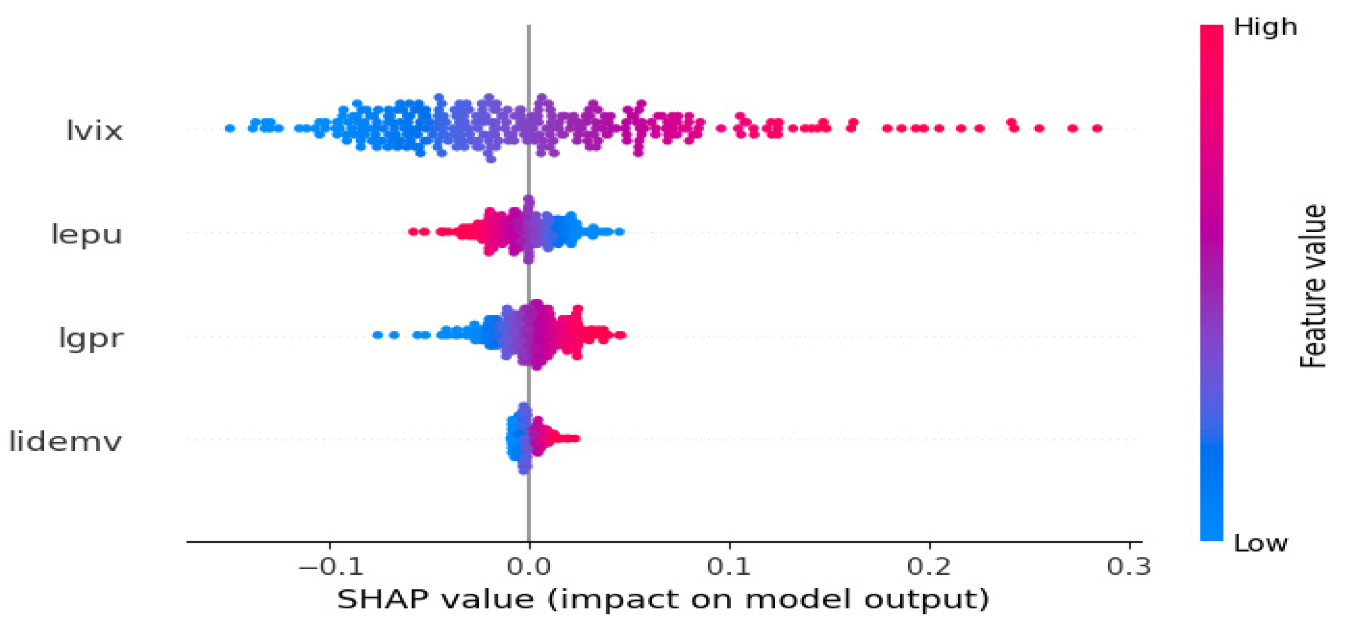
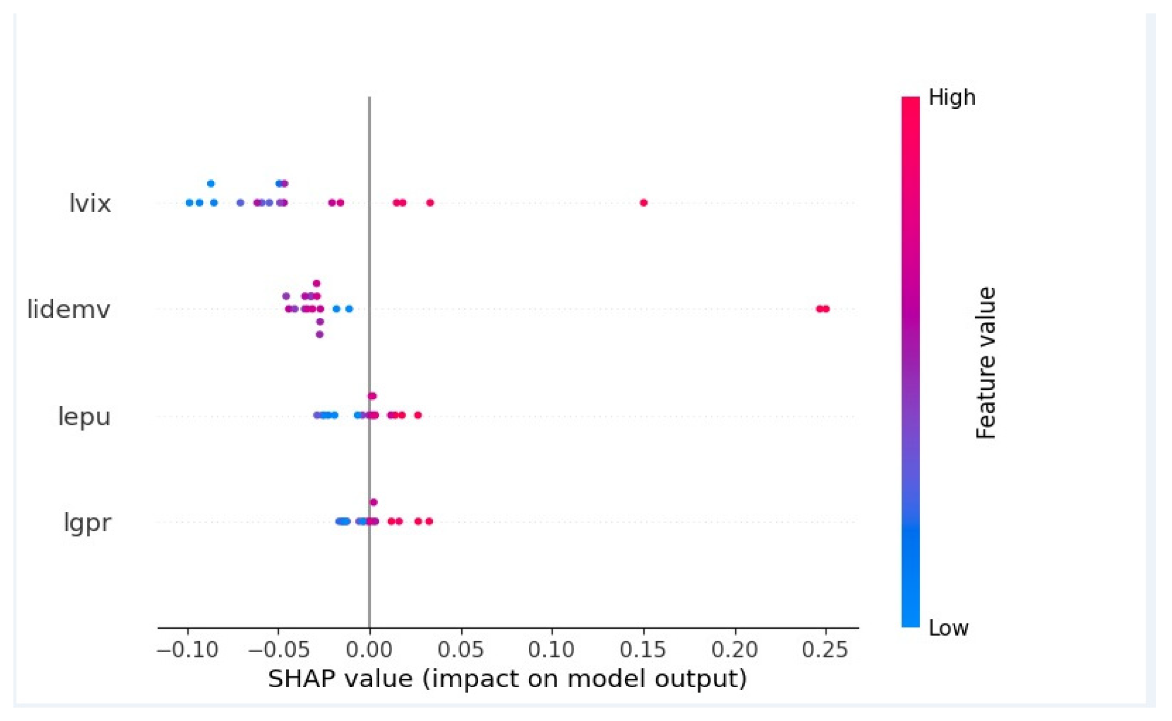
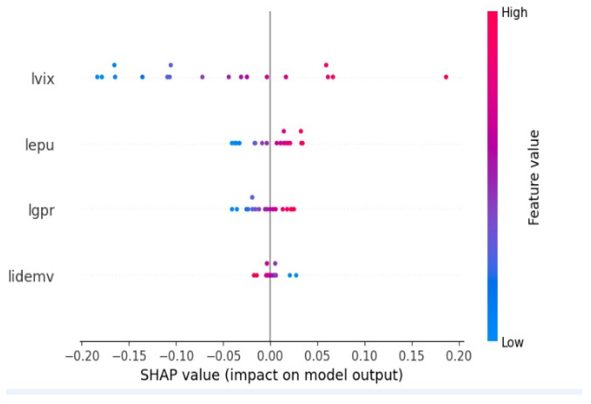
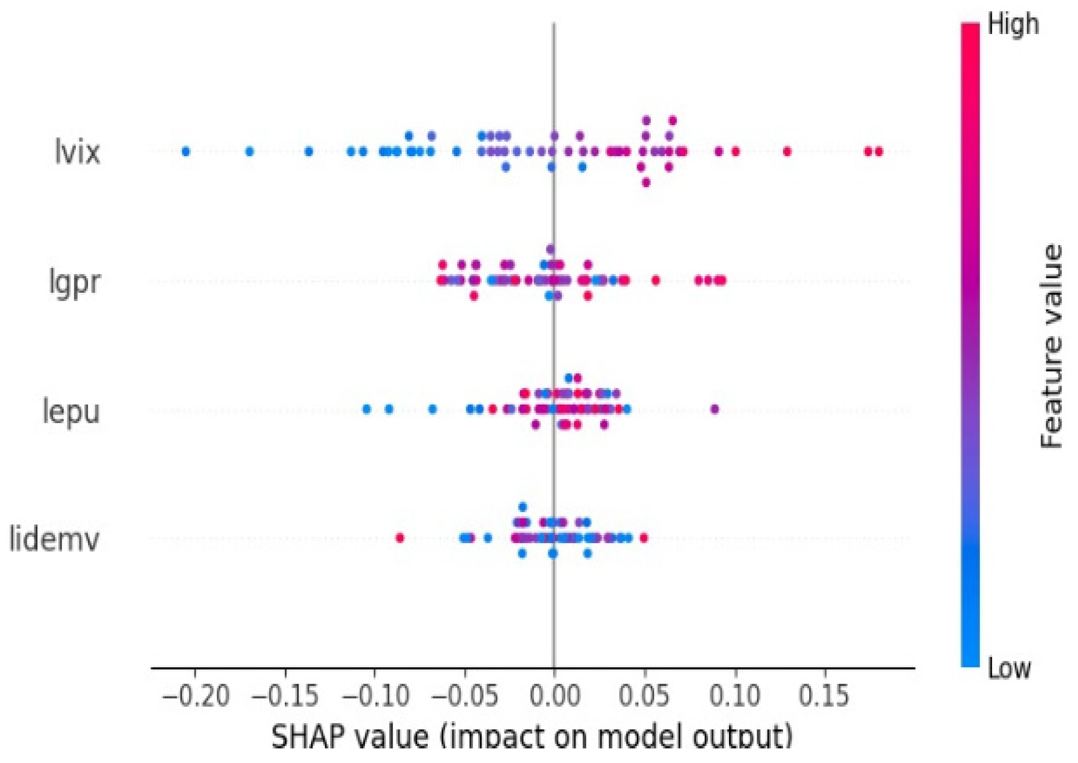
4.2. Feature Importance Analysis

This section presents the features of the prediction generated by the SVM and XGBoost models. The ARIMAX model is excluded from the feature analysis as it provided the worst results. The Shapley Additive Explanation Method is applied to explore the effect of VIX, EPU, GPR, and IDEMV on OVX. Jabeur et al. [15] put forward two reasons for using the SHAP method. First, it is robust to complex relationships between different variables. Second, the SHAP tool allows a better understanding of machine learning results. Before feature evaluation, one of the obvious steps is to interpret the residual convergence of the SVM and XGBoost tools. For this purpose, we use the R package DALEX suggested by Biecek [55]. During the pre-pandemic period, the cumulative inverse distribution of the residual plotted in Figure 5 indicates that the distribution curves of XGBoost and SVM residuals have almost the same pattern, which implies that the residuals of both machine learning methods converge to the optimal solution at the same time during normal times. However, different results were reached during the pandemic. As shown in Figure 6, the XGBoost model performs better than the SVM model with respect to convergence. The residuals converge faster to the optimal solution in the XGBoost model than in the SVM model.

Figure 7, Figure 8, Figure 9 and Figure 10 provide information on the predictive power of the uncertainty indices before and during COVID-19. They show the SHAP values for the SVM and XGBoost models. In the vertical location ($y$-axis), the order of variables appears according to their importance in accurately forecasting the OVX. The shape that is redder means that the feature has a high value, and the shape that is bluer means that the feature has a low value. The horizontal position contains the SHAP values with a higher or lesser impact on the forecast. Furthermore, a positive SHAP value refers to the positive impact of the predictor on the output, while a negative SHAP value refers to a negative impact.

Figure 7 reports the feature importance for the SVM model before the pandemic. It shows that a small VIX value reduces the probability of OVX forecasts by almost 0.2, while a large VIX value increases forecasts by almost 0.3. This result confirms the findings of Bakas and Triantafyllou [34] and Dutta et al. [29] that the implied volatility predicts crude oil volatility. Thus, the positive effect of the VIX on the OVX is more pronounced than its negative effect. However, the OVX forecast increased when there was a fall in EPU of less than 0.1. The effect is the same on the opposite side. For the GPR, it is clear that a small value of GPR was found to decrease the probability of OVX prediction by almost 0.1, while large values of GPR increase the prediction by almost 0.1. These findings are consistent with Liu et al. [35] and Li et al. [26] that the GPR index significantly predicts crude oil volatility.

Finally, the SHAP value of IDEMV tends to be around zero. Referring to these values, the SVM model suggests that the VIX is the most important factor that leads to a positive prediction of OVX. It has the strongest influence on the model. These findings indicate the presence of a significant long-term association between the OVX and VIX. For the other forecasters, the results show a weak effect before the health crisis. This implies that uncertainty in the oil market is mainly affected by uncertainty caused by investor fear in the financial market and subsequently by uncertainty caused by economic policy, geopolitical events, and news about the link between infectious disease and stock market volatility.

Different results are shown for the XGBoost model. Figure 8 shows that the influence of these factors on the prediction of OVX is ambiguous. In more detail, SHAP values of the VIX variable contribute to increasing the probability of OVX prediction by almost 0.2, while a higher VIX value decreases the prediction by almost 0.2. This remains unclear as the results show an overlap between the SHAP values (blue and red shapes). Similar results are also shown for EPU, GPR, and IDEMV. Accordingly, the XGBoost model appears to be limited in providing useful information before COVID-19. Consequently, the SVM model performs better in terms of feature importance during normal times.

To analyze the interaction between OVX and their forecasters during COVID-19, the SHAP importance values derived from the SVM and XGBoost models are plotted in Figure 9 and Figure 10, respectively.

The SVM model (Figure 9) shows that a small value of VIX decreases the probability of the OVX forecasts by almost 0.2. However, a large VIX value increases the forecasts by almost 0.5. This result means that the predictive power of VIX for OVX is improved during the pandemic compared to the pre-pandemic period. Similarly, the prediction of OVX increases when the EPU is below 0.1. However, the SHAP significance analysis shows that when the decrease in EPU is less than 0.1, there is a decrease in the prediction of OVX. Furthermore, the link between OVX and IDEMV becomes evident. Lower IDEMV feature values below 0.1 correspond to a higher probability of OVX. On the contrary, higher IDEMV feature values below 0.1 mean that the probability of OVX decreases. However, the link between OVX and GPR is not evident. Indeed, the SHAP value of the GPR tends to be around zero. For the XGBoost results, Figure 10 shows that the predictive power of the VIX and EPU factors for OVX during the pandemic is improved compared to the pre-pandemic period. Notably, we identify that when features like VIX and EPU reach a high SHAP value, the model is oriented towards positive OVX forecasts. When these features have low SHAP values, the model is oriented towards non-OVX forecasts. These results indicate that the VIX and EPU are the most important features and are consequently considered significant sources of forecasting uncertainty in the oil market during COVID-19. Figure 10 also reveals that SHAP values relative to IDEMV and GPR factors tend to be around zero, suggesting that the predictive power of these features has not been clear during COVID-19.

5. Robustness Check

Robustness analysis is conducted in this section. As predicting crude oil volatility is important for policymakers, energy economists, and financial portfolio managers, we check our findings using weekly frequency data, in line with Ftiti et al. [7]. For the pre-COVID-19 period,

Table 3. A prediction performance assessment of the candidate models (weekly analysis).

Pre-COVID-19				COVID-19
Models	RMSE	MSE	${\mathit{R}}^2$	RMSE	MSE	${\mathit{R}}^2$
XGBoost	0.148	0.021	0.391	0.110	0.012	0.717
SVM	0.128	0.016	0.041	0.153	0.023	0.451

indicates that the performance metrics of the SVM model present the lowest error value for the RMSE and the MSE than those of XGBoost model. This means that the SVM model dominates the XGBoost model in predicting OVX during pre-COVID-19. For the COVID-19 period, Table 3 reports different results. We observe that the performance indicators of the XGboost model are better than those of the SVM model. This illustrates that the OVX index is well forecasted by the XGboost model than the SVM model. In addition, our findings show that the XGboost model is more robust during COVID-19 period than during pre-COVID-19 period. However, this is not the case for SVM model. We report that the performance of SVM model to forecast OVX index is not improved during pandemic conditions compared to pre-COVID-19 conditions. More interestingly, XGboost model remains the best fitting model across all data frequencies (daily and weekly) during the pandemic period.

Figure 11, Figure 12, Figure 13 and Figure 14 plot the predictive power of the uncertainty indices before and during COVID-19 using weekly frequency data. In the pre-COVID-19 period, the SVM and the XGBoost models (Figure 11 and Figure 12) confirm the daily findings that the VIX is the most important factor that leads to a positive prediction of OVX. It has the strongest influence on the model. These findings indicate the presence of a significant long-term association between the OVX and VIX. Also, this effect is more pronounced by the XGBoost model more than the SVM model. Similar results are also shown during the pandemic period. Both machine learning tools (Figure 13 and Figure 14) highlight that the VIX index is the most important features to have a significant source of forecasting uncertainty in the oil market during COVID-19 pandemic.

6. Concluding Remarks and Implications

There is a consensus among traders, policymakers, and academics that oil market uncertainty has substantial implications for optimal portfolio management, economic activity, and financial markets [56]. So, what we have noticed through the in-depth study of the literature review focusing on the oil market uncertainty is the existence of a research gap concerning the lack of studies that focused on the predictive power of different uncertainty measures for the crude oil volatility. In response to this, this paper tries to examine the predictive performance of various uncertainty indices related to news on the infectious diseases-stock market volatility linkage, financial market, economic policy, and geopolitical events for forecasting the crude oil volatility index be-fore and during the COVID-19 outbreak. To investigate such complex associations, we use two competing machine learning models: the Support Vector Machine and the XGBoost against the Autoregressive integrated moving average ARIMAX (p,d,q) model. The aim is to determine which model performs better in predicting the crude oil volatility index before and during the recent health crisis.

The analysis provides interesting results compared to the existing literature. In terms of accuracy, the forecasting results show that the SVM model dominates the XGBoost model in predicting the OVX index before COVID-19. In addition, the used performance metrics reveal the superiority of the SVM model. Nevertheless, the results are different when the COVID-19 pandemic took place. The results reveal that the XGBoost model outperforms the SVM model in predicting the OVX index. In terms of convergence, applying the inverse cumulative distribution of the residuals shows that both machine learning models generate good convergence. The results reveal that residuals converge to the optimal solution for the XGBoost model faster than for the SVM model. In terms of feature importance, the analysis performed using the Shapley Additive Explanation Method reveals important results. Before the COVID-19 outbreak, the SVM model results indicate that uncertainty in the oil market was mainly affected by uncertainty caused by investor fear in the financial market, followed by economic policy uncertainty, geopolitical risk, and news on the infectious diseases-stock market volatility linkage. On the other hand, the XGBoost appears to be limited in providing useful information during normal times. During COVID-19, the results indicate that the predictive power of the VIX and EPU factors for the forecasting of OVX is improved compared to pre-COVID-19. This suggests that uncertainty caused by investor fear in the financial market and economic policy uncertainty are the most important features and are consequently considered significant sources of uncertainty in the oil market. Our results are proven as robust whatever the frequency of the data (daily or weekly).

The above results have important policy implications for policymakers, energy economists, and financial portfolio managers. First, the significant effect of VIX and EPU on OVX indicates that energy market regulators should adopt appropriate measures to limit the transmission of financial market and economic policy uncertainty shocks. This strategy will improve confidence in the oil market and thus market sentiment. Risk sentiment will also increase, which is immediately reflected in the rise of crude oil futures. From this perspective, inexperienced traders should not consider these contracts as investment tools and apply investment rules known as other investment tools, such as stocks. Similarly, traders should know that they are trading on a short-term time horizon, and before the settlement date, they must have gotten rid of the contract unless they want to receive oil with a place to store it. Indeed, this helps policymakers to be certain that the achievement of a stable energy market is mainly related to the governance, control of oil futures contracts and limit investors fear.

Second, the high uncertainty in the oil market during COVID-19 compared to normal periods means that the perspectives of energy markets and economic growth generally became more ambiguous due to the health crisis. Uncertainty in the oil market is not only about prices but also about demand and the medium- and long-term perspectives of the oil industry. Given the continuing uncertainty in the market, policymakers and energy economists need to adjust oil production strategies. Third, knowledge of the main sources of uncertainty in the oil market before and during COVID-19 allows financial portfolio managers and traders to choose the appropriate time to buy or sell their oil futures contracts. Finally, the effectiveness of machine learning techniques pushes authorities in charge of financial and energy policy to utilize these sophisticated tools to forecast uncertainty and other risky assets.

Although this study presents important results and policy implications for investors and policymakers, it has some limitations. First, this research did not consider the COVID-19 pandemic as a possible factor in the linkage between uncertainty and OVX. Second, the research does not consider uncertainty measures related to other commodity markets. The empirical evidence of this study can be improved by considering these limitations. Future research can implement new deep learning algorithms and more predictive uncertainty predictors.

References

1. Le, D.T. Ex-ante determinants of volatility in the crude oil market. Int. J. Financ. Res. 2014, 6, 1–13. [Google Scholar] [CrossRef] [Green Version]
2. Narayan, P.K.; Ranjeeni, K.; Bannigidadmath, D. New evidence of psychological barrier from the oil market. J. Behav. Financ. 2017, 18, 457–469. [Google Scholar] [CrossRef]
3. Shahzad, S.J.; Naifar, N.H.; Hammoudeh, S.; Roubaud, D. Directional predictability from oil market uncertainty to sovereign credit spreads of oil-exporting countries: Evidence from rolling windows and crossquantilogram analysis. Energy Econ. 2017, 68, 327–339. [Google Scholar] [CrossRef]
4. Wheeler, C.M.; Baffes, J.; Kabundi, A.; Kindberg-Hanlon, G.; Nagle, P.S.; Ohnsorge, F. Adding Fuel to the Fire: Cheap Oil during the COVID-19 Pandemic; Policy Research Working Papers 9320; The World Bank: Washington, DC, USA, 2020. [Google Scholar]
5. Devpura, N.; Narayan, P.K. Hourly oil price volatility: The role of COVID-19. Energy Res. Lett. 2020, 1, 13683. [Google Scholar] [CrossRef]
6. Charles, A.; Darné, O. Forecasting crude-oil market volatility: Further evidence with jumps. Energy Econ. 2017, 67, 508–519. [Google Scholar] [CrossRef]
7. Ftiti, Z.; Tissaoui, K.; Boubaker, S. On the relationship between oil and gas markets: A new forecasting framework based on a machine learning approach. Ann. Oper. Res. 2020, 313, 915–943. [Google Scholar] [CrossRef]
8. Wu, B.; Wang, L.; Wang, S.; Zeng, Y.-R. Forecasting the U.S. oil markets based on social media information during the COVID-19 pandemic. Energy 2021, 226, 120403. [Google Scholar] [CrossRef]
9. Jo, S. The Effects of Oil Price Uncertainty on Global Real Economic Activity. J. Money Credit Bank. 2014, 46, 1113–1135. [Google Scholar] [CrossRef]
10. Assaf, A.; Charif, H.; Mokni, K. Dynamic connectedness between uncertainty and energy markets: Do investor sentiments matter? Resour. Policy 2021, 72, 102112. [Google Scholar] [CrossRef]
11. Echaust, K.; Just, M. Tail Dependence between Crude Oil Volatility Index and WTI Oil Price Movements during the COVID-19 Pandemic. Energies 2021, 14, 4147. [Google Scholar] [CrossRef]
12. Bourghelle, D.; Jawadi, F.; Rozin, P. Oil price volatility in the context of COVID-19. Int. Econ. 2021, 167, 39–49. [Google Scholar] [CrossRef]
13. Christopoulos, A.G.; Kalantonis, P.; Katsampoxakis, I.; Vergos, K. COVID-19 and the Energy Price Volatility. Energies 2021, 14, 6496. [Google Scholar] [CrossRef]
14. Chen, T.; Guestrin, C. XGBoost: A Scalable Tree Boosting System. In Proceedings of the 22nd ACM SIGKDD International Conference on Knowledge Discovery and Data Mining, San Francisco, CA, USA, 13–17 August 2016; ACM: New York, NY, USA, 2016; pp. 785–794. [Google Scholar]
15. Jabeur, S.B.; Khalfaoui, R.; Arfi, W.B. The effect of green energy, global environmental indexes, and stock markets in predicting oil price crashes: Evidence from explainable machine learning. J. Environ. Manage 2021, 298, 113511. [Google Scholar] [CrossRef] [PubMed]
16. Wu, J.; Miu, F.; Li, T. Daily crude oil price forecasting based on improved CEEMDAN, SCA, and RVFL: A case study in WTI oil market. Energies 2020, 13, 1852. [Google Scholar] [CrossRef] [Green Version]
17. Hamilton, J.D. Oil and the macroeconomy since World War II. J. Polit. Econ. 1983, 91, 228–248. [Google Scholar] [CrossRef]
18. Kilian, L.; Park, C. The impact of oil price shocks on the U.S. stock market. Int. Econ. Rev. 2009, 50, 1267–1287. [Google Scholar] [CrossRef]
19. Coleman, L. Explaining crude oil prices using fundamental measures. Energy Policy 2012, 40, 318–324. [Google Scholar] [CrossRef]
20. Pan, Z.; Wang, Y.; Wu, C.; Yin, L. Oil price volatility and macroeconomic fundamentals: A regime switching GARCH-MIDAS model. J. Empir. Financ. 2017, 43, 130–142. [Google Scholar] [CrossRef]
21. Demirer, R.; Ferrer, R.; Shahzad, S.J.H. Oil price shocks, global financial markets and their connectedness. Energy Econ. 2020, 8, 104771. [Google Scholar] [CrossRef]
22. Sadorsky, P. Oil price shocks and stock market activity. Energy Econ. 1999, 21, 449–469. [Google Scholar] [CrossRef]
23. Hammoudeh, S.; Huimin, L. Oil sensitivity and systematic risk in oil-sensitive stock indices. J. Econ. Bus. 2005, 57, 1–21. [Google Scholar] [CrossRef]
24. Frankel, J.A. Commodity Prices, Monetary Policy, and Currency Regimes. NBER Working Paper No. C0011. 2006. Available online: https://users.nber.org/~confer/2006/apmps06/frankel.pdf (accessed on 20 October 2021).
25. Wang, Y.; Wu, C. Energy prices and exchange rates of the US dollar: Further evidence from linear and nonlinear causality analysis. Econ. Model. 2012, 29, 2289–2297. [Google Scholar] [CrossRef]
26. Li, R.; Hu, Y.; Heng, J.; Chen, X. A novel multiscale forecasting model for crude oil price time series. Technol. Forecast. Soc. Change 2021, 173, 121181. [Google Scholar] [CrossRef]
27. Zhao, L.-T.; Zeng, G.-R.; Wang, W.-J.; Zhang, Z.-G. Forecasting Oil Price Using Web-based Sentiment Analysis. Energies 2019, 12, 4291. [Google Scholar] [CrossRef] [Green Version]
28. Orzeszko, W. Nonlinear Causality between Crude Oil Prices and Exchange Rates: Evidence and Forecasting. Energies 2021, 14, 6043. [Google Scholar] [CrossRef]
29. Dutta, A.; Bouri, E.; Saeed, T. News-based equity market uncertainty and crude oil volatility. Energy 2021, 222, 119930. [Google Scholar] [CrossRef]
30. Baker, S.R.; Bloom, N.; Davis, S.J. Uncertainty and the economy. Policy Rev. 2012, 175, 3. [Google Scholar]
31. Bekiros, S.; Gupta, R.; Majumdar, A. Incorporating economic policy uncertainty in US equity premium models: A nonlinear predictability analysis. Financ. Res. Lett. 2016, 18, 291–296. [Google Scholar] [CrossRef] [Green Version]
32. Wei, Y.; Liu, J.; Lai, X.; Hu, Y. Which determinant is the most informative in forecasting crude oil market volatility: Fundamental, speculation, or uncertainty? Energy Econ. 2017, 68, 141–150. [Google Scholar] [CrossRef]
33. Ma, R.; Zhou, C.; Cai, H.; Deng, C. The forecasting power of EPU for crude oil return volatility. Energy Rep. 2019, 5, 866–873. [Google Scholar] [CrossRef]
34. Bakas, D.; Triantafyllou, A. Volatility forecasting in commodity markets using macro uncertainty. Energ. Econ. 2019, 81, 79–94. [Google Scholar] [CrossRef]
35. Yang, L. Connectedness of economic policy uncertainty and oil price shocks in a time domain perspective. Energy Econ. 2019, 80, 219–233. [Google Scholar] [CrossRef]
36. Qin, Y.; Hong, K.; Chen, J.; Zhang, Z. Asymmetric effects of geopolitical risks on energy returns and volatility under different market conditions. Energy Econ. 2020, 90, 104851. [Google Scholar] [CrossRef]
37. Liu, J.; Ma, F.; Tang, Y.; Zhang, Y. Geopolitical risk and oil volatility: A new insight. Energy Econ. 2019, 84, 104548. [Google Scholar] [CrossRef]
38. Mei, D.; Ma, F.; Liao, Y.; Wang, L. Geopolitical risk uncertainty and oil future volatility: Evidence from MIDAS models. Energy Econ. 2020, 86, 104624. [Google Scholar] [CrossRef]
39. Tiwari, A.K.; Aye, G.C.; Gupta, R.; Gkillas, K. Gold-Oil Dependence Dynamics and the Role of Geopolitical Risks: Evidence from a Markov-Switching Time-Varying Copula Model. Energy Econ. 2020, 88, 104748. [Google Scholar] [CrossRef]
40. Nonejad, N. Forecasting crude oil price volatility out-of-sample using news-based geopolitical risk index: What forms of nonlinearity help improve forecast accuracy the most? Financ. Res. Lett. 2021, 46, 102310. [Google Scholar] [CrossRef]
41. Lu, X.; Ma, F.; Li, P.; Li, T. Newspaper-based equity uncertainty or implied volatility index: New evidence from oil market volatility predictability. Appl. Econ. Lett. 2022. Available online: https://www.tandfonline.com/doi/abs/10.1080/13504851.2022.2030459. (accessed on 1 June 2022).
42. Bouri, E.; Demirer, R.; Gupta, R.; Pierdzioch, C. Infectious diseases, market uncertainty and oil market volatility. Energies 2020, 13, 4090. [Google Scholar] [CrossRef]
43. Whaley, R.E. Derivatives on market volatility: Hedging tools long overdue. J. Deriv. 1993, 1, 71–84. [Google Scholar] [CrossRef]
44. Tissaoui, K. Forecasting implied volatility risk indexes: International evidence using Hammerstein-ARX approach. Int. Rev. Financ. Anal. 2019, 64, 232–249. [Google Scholar] [CrossRef]
45. Hao, X.; Zhao, Y.; Wang, Y. Forecasting the real prices of crude oil using robust regression models with regularisation constraints. Energy Econ. 2020, 86, 104683. [Google Scholar] [CrossRef]
46. Vapnik, V.N. The support vector method. In Proceedings of the International Conference on Artificial Neural Networks, Houston, TX, USA, 12 June 1997; Springer: Berlin/Heidelberg, Germany, 1997; pp. 261–271. [Google Scholar]
47. Smola, A.J.; Scholkopf, B. A tutorial on support vector regression. Stat. Comput. 2004, 14, 199–222. [Google Scholar] [CrossRef] [Green Version]
48. Kuhn, H.W.; Tucker, A.W. Nonlinear Programming. In Proceedings of the 2nd Berkeley Symposium on Mathematical Statistics and Probability, Berkeley, CA, USA, 31 July–12 August 1950; University of California Press: Berkeley, CA, USA, 1951; pp. 481–492. [Google Scholar]
49. Ostrowski, K.; Birman, K. Extensible web services architecture for notification in large-scale systems. In Proceedings of the 2006 IEEE International Conference on Web Services (ICWS’06), Chicago, IL, USA, 18–22 September 2006; pp. 383–392. [Google Scholar]
50. Singh, N.; Singh, P.; Bhagat, D. A rule extraction approach from support vector machines for diagnosing hypertension among diabetics. Expert Syst. Appl. 2019, 130, 188–205. [Google Scholar] [CrossRef]
51. Ma, B.; Meng, F.; Yan, G.; Yan, H.; Chai, B.; Song, F. Diagnostic classification of cancers using extreme gradient boosting algorithm and multiomics data. Comput. Biol. Med. 2020, 121, 103761. [Google Scholar] [CrossRef]
52. Lundberg, S.M.; Lee, S.I. A unified approach to interpreting model predictions. In Proceedings of the Advances in Neural Information Processing Systems, Long Beach, CA, USA, 4–9 December 2017; pp. 4765–4774. [Google Scholar]
53. Shapley, L.S. A value for n-person games. In Contributions to the Theory of Games; Princeton University Press: Princeton, NJ, USA, 1953; pp. 307–317. [Google Scholar] [CrossRef]
54. Tissaoui, K.; Azibi, J. International implied volatility risk indexes and Saudi stock return-volatility predictabilities. N. Am. J. Econ. Financ. 2018, 47, 65–84. [Google Scholar] [CrossRef]
55. Biecek, P. DALEX: Explainers for complex predictive models in R. J. Mach. Learn. Res. 2018, 19, 3245–3249. [Google Scholar]
56. Tissaoui, K.; Zaghdoudi, T. Dynamic connectedness between the US financial market and Euro-Asian financial markets: Testing transmission of uncertainty through spatial regressions models. Q. Rev. Econ. Financ. 2020, 81, 481–492. [Google Scholar] [CrossRef]
Figure 1. Correlation analysis before COVID-19. Notes: (*) Significant at the 10%; and (***) Significant at the 1%.
Energies 15 05744 g001
Figure 2. A correlation analysis during COVID-19. Notes: (**) Significant at the 5%; and (***) Significant at the 1%.
Energies 15 05744 g002
Figure 3. A plot of OVX forecasts before COVID-19.
Energies 15 05744 g003
Figure 4. A plot of OVX forecasts during COVID-19.
Energies 15 05744 g004
Figure 5. Reverse cumulative distribution of residuals during the pre-COVID-19 period.
Energies 15 05744 g005
Figure 6. The reverse cumulative distribution of residuals during the COVID-19 period.
Energies 15 05744 g006
Figure 7. Feature importance before the pandemic—SVM model (Daily frequency).
Energies 15 05744 g007
Figure 8. Feature importance before the pandemic—XGBoost model (Daily frequency).
Energies 15 05744 g008
Figure 9. The SVM model: Feature importance during the pandemic (Daily frequency).
Energies 15 05744 g009
Figure 10. The XGBoost model: Feature importance during the pandemic (Daily frequency).
Energies 15 05744 g010
Figure 11. Feature importance before the pandemic—SVM model (Weekly frequency).
Energies 15 05744 g011
Figure 12. Feature importance before the pandemic—XGBoost model (Weekly frequency).
Energies 15 05744 g012
Figure 13. Feature importance during the pandemic—SVM model (Weekly frequency).
Energies 15 05744 g013
Figure 14. Feature importance during the pandemic—XGBoost model (Weekly frequency).
Energies 15 05744 g014