Implementation and Analyses of an Eco-Driving Algorithm for Different Battery Electric Powertrain Topologies Based on a Split Loss Integration Approach

Abstract

Eco-driving algorithms optimize the speed profile to reduce the energy consumption of a vehicle. This paper presents an eco-driving algorithm for battery electric powertrains that applies a split loss integration approach to incorporate the component losses. The algorithm consistently uses loss models to overcome the drawbacks of efficiency maps, which cannot represent no-load losses at zero torque. The use of loss models is crucial since the optimal solution includes gliding, during which there are no-load losses. An analysis shows, that state-of-the-art nonlinear programming algorithms cannot represent these no-load losses at zero torque with a small modeling error. To effectively compute the powertrain losses with only a small error in comparison to the measurement data, we introduce a tailored combination of nonlinear inequality constraints that interleave two polynomial fits. This approach can properly represent reality. We parameterize the algorithm and validate the vehicle model used with real-world measurement data. Furthermore, we investigate the influence of the proposed interleaved fits by comparing them to a single continuous high-order polynomial fit and to the state of the art. The algorithm is published open source.

1. Introduction

A reduction in energy demand and emissions as well as mitigating traffic congestion represent outstanding challenges. Connected, automated and electric vehicles may change an individual transport system. BEV eliminate tailpipe emissions. Nevertheless, their battery capacity, and hence their range, is limited. The automation of BEV may exacerbate this effect because auxiliary power consumption increases due to the higher computational demand [1]. However, connected and automated vehicles may increase traffic efficiency and therefore decrease energy demand [2,3] as well as improving the energy efficiency of the vehicle itself by adapting its driving behavior [4], which could reduce the drawbacks of BEV.

Improving energy efficiency and consequently the range of BEV can be divided into two areas: vehicle design and vehicle operation. Energy-efficient driving saves energy during operation, however, the boundary conditions are set during the vehicle conceptual phase. In the conceptual phase the energy demand of the vehicle can be influenced by selecting the powertrain topology and choosing and sizing the powertrain components [5,6,7,8,9]. In our previous studies, we have shown that the powertrain topology affects the optimal speed profile of the vehicle and the resulting energy demand [10]. The joint optimization of the powertrain and speed profile are addressed in [11,12]. However, the topologies considered and driving scenarios are limited. For an electric race car, Borsboom et al. [13] optimize the powertrain size and the speed profile for a transmission with a fixed gear ratio and a CVT. However, their objective is a minimum lap time and their powertrain topology is fixed.

Eco-driving describes a wide range of measures to make road transport more ecological. Huang et al. [14] presented different definitions and scopes of eco-driving found in the literature, including vehicle selection, route planning, driving style, cabin comfort, and maintenance. A similar classification is given in [15]. Huang et al. [14] focus on driving behavior: speed, acceleration, deceleration, route choice, idling, and accessories. Where speed is concerned, they propose a constant speed as the optimal energy-efficient speed profile. However, optimizing approaches reveal that, due to poor efficiency at low load, cruising may not be as efficient as a periodic alternation between acceleration and coasting [10,16,17,18], both for combustion engines and electric motors. This driving strategy is also called P&G.

Energy-optimal speed profiles differ in the literature, depending on the boundary conditions and on the formulation of the optimization problem. In our previous paper [10], we differentiated between the objective function formulations, which included

• Minimization of squared acceleration;
• “Wheel-to-distance” energy minimization;
• “Tank-to-distance” energy minimization.

In the following, the different objectives are discussed in detail.

1.1. Minimization of Squared Acceleration

The minimization of squared acceleration does not minimize energy but acceleration. In many cases, acceleration correlates with the energy required. However, the P&G example shows that this is not always the case. The advantage is fast calculations. Examples are given in [19,20,21,22].

1.2. Wheel-to-Distance Energy Minimization

Wheel-to-distance energy minimizations minimize the required energy at the wheel. Thus, air, roll, inclination and inertial resistance are minimized. Assuming a given vehicle, the route choice and speed are the main levers for optimizing energy consumption. Han et al. [16] present a wheel-to-distance optimal speed profile. In general, the optimal wheel-to-distance speed profile consists of a fast acceleration/deceleration followed by a constant speed until close to the destination. Deceleration should include coasting but can also consist of harsh braking.

1.3. Tank-to-Distance Energy Minimization

Since all losses are relevant to the total energy demand of a vehicle, tank-to-distance energy minimizations have the largest potential to save energy since they incorporate all losses from the tank or battery up to the conversion into distance covered. The minimization of tank-to-distance energy consumption represents an optimal control problem (OCP). Diehl et al. [23] name dynamic programming (DP), direct methods and indirect methods as the three basic approaches to solving OCP, whereas direct methods are the most widespread for real-world problems. Direct methods use nonlinear programming (NLP), whereby numerical methods can be categorized into gradient-based methods and heuristic methods [24]. Below, the literature relating to eco-driving with a defined electric powertrain is analyzed. In doing so, we differentiate between optimizations using DP and direct methods with gradient-based numerical methods.

1.3.1. Optimizations Using Dynamic Programming

DP is used to optimize speed profiles for electric vehicles [11,17,25], electric buses [18,26] or electric trains [27].

Lin et al. [25] used DP to develop a driving assistance system based on speed profile optimization. The powertrain is modeled with a constant transmission efficiency, a motor efficiency map, and a Rint model representing the battery. So et al. [17] implemented an eco-driving algorithm, using DP. The case study is a lightweight vehicle. Motor and power electronics are modeled by an efficiency map. Since the vehicle has in-wheel motors, no transmission is modeled. Anselma and Belingardi [11] used a DP algorithm to optimize the speed profiles of electric vehicles by simultaneously optimizing the powertrain. The transmission is modeled as a constant efficiency. The authors state that they use empiric loss maps to model the motor, however, in their equations, they use load-point-dependent efficiencies for the motor and inverter. They model the battery with a Rint model. In [18], we implemented a DP, algorithm and optimized speed profiles for electric buses, varying gear ratio, and motor type. Constant transmission efficiency and motor efficiency maps were used. The battery and inverter were neglected. Liao et al. [28] implemented a temperature-dependent battery in their powertrain. They used a Rint model with temperature-dependent open-circuit voltage (OCV) and internal resistance. Motor and CVT are modeled as fits of efficiency maps. Franke et al. [27] used loss maps to model the electric motor. However, since the research of Franke et al. relates to trains, the boundary conditions differ.

1.3.2. Optimizations Using Direct Methods

Shao (p. 93ff [29]) presented NLP for a BEV with an IM. The power of the drivetrain $P_{\mathrm{drv}}$ is modeled by a polynomial as a function of motor speed and torque

$$P_{\mathrm{drv}}=p_{00}+p_{10}{\omega }_{\mathrm{m}}+p_{10}{T}_{\mathrm{m}}+p_{11}{\omega }_{\mathrm{m}}{T}_{\mathrm{m}}$$

(1)

with fitting coefficients $p_{ij}$, motor speed ${\omega }_{\mathrm{m}}$ and motor torque $T_{\mathrm{m}}$. He used a Rint battery model. The constraints he applied included jerk limitations, speed limitations, distance to leading vehicle limitations, regenerative braking constraints based on the state of charge (SOC) and vehicle speed, braking force balance constraints and discharging constraints. The algorithm was implemented in Matlab and uses the interior-point solver IPOPT [30].

For an energy-optimal adaptive cruise control, Jia et al. [31] presented two algorithms, a linearly constrained quadratic programming algorithm in the time domain and an NLP algorithm in the space domain. Assuming constant transmission efficiency and a single-speed transmission, the power consumption is a function of traction force $F_{\mathrm{t}}$ and vehicle speed v for a specific SOC. The power is fitted by a polynomial with

$$P=p_{00}+p_{10}v+p_{10}{F}_{\mathrm{t}}+p_{11}v{F}_{\mathrm{t}}+p_{20}{v}^2+p_{02}{F}_{\mathrm{t}}^2$$

(2)

For the space domain, power demand per meter is fitted as a function of traction force and the square of velocity. This results in a more accurate fit than in the time domain.

Bertoni et al. [32] proposed an energy-efficient adaptive cruise control for connected electric vehicles. They used a variable air drag coefficient based on the inter-vehicle distance based on experimental data from [33]. To model the powertrain, they fitted the electric motor power by

$$P_{\mathrm{m}}=p_{11}{\omega }_{\mathrm{m}}{T}_{\mathrm{m}}+p_{02}{T}_{\mathrm{m}}^2,$$

(3)

based on a scaled motor efficiency map and a transmission efficiency of 90%. Battery internal losses were neglected. Again, this problem was solved with IPOPT.

Schwickart et al. [34] implemented a real-time energy-efficient model-predictive cruise controller for an electric vehicle. The cost function consists of the squared energy consumption which itself is modeled by fitting six planes to the electrical energy per meter. The planes are incorporated into the algorithm by inequality constraints.

He et al. [35] used sequential quadratic programming (SQP) to enable eco-driving for an electric sightseeing vehicle. Regarding the powertrain, they only implemented motor current losses based on the current I, which itself is assumed to be linearly dependent on the motor traction force F

$$P_{\mathrm{c}}=R{I}^2=R{\left(cF\right)}^2,$$

(4)

with the current losses $P_{\mathrm{c}}$, winding resistance R and constant c.

We demonstrated in our previous research [10], that quadratic representations of power are not sufficient for powertrains with multiple motors or multiple gears as these fits are not suitable for finding the most efficient operation mode. We introduced higher polynomial fits, for traction and recuperation each with

$$P=\sum _{y=0}^n\sum _{x=0}^{m-y}{p}_{xy}{\omega }_{\mathrm{m}}^x{T}_{\mathrm{m}}^y$$

(5)

while we used fits of degree $m=6$ and $n=6$. The transmission was represented as a constant efficiency, and battery and power electronics were neglected.

1.4. Review of Existing Algorithms and Scope of the Paper

Even though the usage of loss maps for motor and gearbox can be considered to be state-of-the-art in simulation applications [7], their consistent usage has not been seen in optimization applications. In [17,18], it is shown, that P&G, can help BEV to achieve a lower energy consumption than at constant speed because the high torque during acceleration corresponds to high motor efficiency. These papers use efficiency maps to model the motor losses and constant transmission efficiencies. However, with this implementation, losses at zero torque (and zero speed) cannot be represented (p. 56 [7]). Thus, no-load losses during gliding are neglected. Approaches that used fitting approaches [29,31,32,34] may have included no-load losses at zero torque, however, they use low-degree polynomials to fit the losses. We will show, that these fits are not capable of representing the actual losses of the vehicle. As these fits are used in the eco-driving optimization algorithms, the obtained solutions are sub-optimal. Since different powertrain topologies and motors may also make it possible to reduce the energy demand of BEV, these levers should also be considered. Finally, the hypothesis of the paper is an eco-driving algorithm that outperforms the current algorithms with respect to model accuracy by using detailed loss models and their innovative integration into the algorithm. Thereby, the algorithm gains more energy savings than other algorithms for battery electric powertrains. Additionally, the algorithm’s predicted powertrain states and energy-saving potential shall coincide with our real-world measurements. Thus, the scope of the paper is:

• To formulate an online capable eco-driving algorithm that consistently uses losses instead of efficiencies for all relevant powertrain components in order to include the powertrain’s no-load losses at zero torque in the optimization. To fit the losses with only a small error, especially in the region at zero torque, we introduce a tailored combination of nonlinear inequality constraints.
• To formulate an eco-driving algorithm that can handle different powertrain topologies and incorporate the powertrain in a component-wise manner, so that the effect of different powertrain components, such as different motors or transmission configurations, can be addressed
• To implement a transmission loss model
• To parameterize and validate the algorithm with real-world data

The remainder of the paper is structured as follows: in Section 2, we give an overview of loss modeling of wheel-to-distance losses and battery-to-wheel losses. Based on the overview, we set our assumptions and propose an eco-driving algorithm that uses loss models in Section 3. Furthermore, we present the conducted experiments. In Section 4, the algorithm is parameterized. The results and an interpretation are presented in Section 5, which focuses on the validity of the models and meta-models and presents a comparison to the state-of-the-art.

2. Preliminaries on Powertrain Loss Modeling

Optimal speed profiles depend on the modeling techniques used for the powertrain components and their power losses. In this section, we provide an overview of modeling the energy losses of a BEV. We differentiate between wheel-to-distance losses and battery-to-wheel losses.

2.1. Wheel-to-Distance Losses

When moving, the vehicle experiences forces, namely air resistance, rolling resistance, gravity and inertial force.

Aerodynamic forces arise due to the viscous friction of the surrounding air acting on the vehicle surface and due to a pressure difference between the front and the rear of the vehicle (p. 14f [36]). Equation (6) is commonly used to calculate the air resistance force:

$$F_{\mathrm{air}}=0.5{\rho }_{\mathrm{a}}{c}_{\mathrm{a}}{a}_{\mathrm{a}}{v}_{\mathrm{flow}}^2,$$

(6)

with air density ${\rho }_{\mathrm{a}}$, vehicle front surface $a_{\mathrm{a}}$, aerodynamic drag coefficient $c_{\mathrm{a}}$, and incident velocity $v_{\mathrm{flow}}$.

On tarmac roads, the rolling resistance is mainly due to flexing losses of the wheel (p. 50 [37]). The roll resistance force depends on the tire load, resulting in

$$F_{\mathrm{roll}}=f_{\mathrm{r}}{F}_{\mathrm{z}},$$

(7)

with the rolling resistance coefficient $f_{\mathrm{r}}$ and the tire load $F_{\mathrm{z}}$. In many longitudinal simulations, $f_{\mathrm{r}}$ is assumed to be constant, however, its value depends on velocity, pressure, and temperature. A measuring method is proposed in SAE J 2452 [38] for determining the rolling resistance. It is proposed to model the rolling resistance by

$$F_{\mathrm{roll}}=F_{\mathrm{z}}^{\alpha }{P}_{\mathrm{tire}}^{\beta }\left(a+bv+c{v}^2\right),$$

(8)

with inflation pressure $P_{\mathrm{tire}}$ and the fitting coefficients $\alpha$, $\beta$, a, b and c [39]. Others have shown that cold tires increase the rolling resistance [40,41].

On inclined roads, the vehicle must overcome the force due to gravity (p. 16 [36]). The force can be modeled by

$$F_{\mathrm{slope}}=m_{\mathrm{veh}}g\sin (\alpha ),$$

(9)

with the vehicle’s mass $m_{\mathrm{veh}}$, acceleration due to gravity g and road gradient $\alpha$. In contrast to the resistance forces referred to above, this force acts either in or against the direction of travel.

During acceleration, an additional force is required. However, it is not only necessary to accelerate the mass of the vehicle but also its rotating parts, such as the wheels, shafts, gears and the rotor of the motor (p. 16f [36], p. 79ff [42]). The drivetrain inertia $I_{DT}$ can be calculated as being equal to an equivalent mass $m_{\mathrm{eq}}$. The equivalent mass of rotating parts can also be expressed by means of the factor $\lambda$ (p. 82 [42]) resulting in a required force

$$F_{\mathrm{acc}}=\left(m_{\mathrm{veh}}+\frac{I_{\mathrm{DT}}}{r_{\mathrm{w}}^2}\right)a=(m_{\mathrm{veh}}+m_{\mathrm{eq}})a=m_{\mathrm{veh}}\lambda a,$$

(10)

with acceleration a and wheel radius $r_{\mathrm{w}}$. The equivalent mass $m_{\mathrm{eq}}$ depends on the powertrain and the selected gear. For passenger cars with combustion engines, $\lambda$ ranges from $1.05$ to $1.5$, depending on the selected gear (p. 82 [42]). Most BEV have single-speed transmissions. Thus, $\lambda$ does not vary. By reverse engineering, Steinstraeter et al. [43] estimated a drivetrain inertia of 10.42 kgm${}^2$ for a BEV based on BMW i3 and Tesla Model 3 components.

2.2. Battery-to-Wheel Losses

The total of the wheel-to-distance forces is provided by the powertrain and brakes. Here, battery, inverter, motor and gearbox losses are relevant. As these losses are load-point-dependent, simulations often use efficiency or loss maps. However, efficiency maps cannot represent load-independent losses at zero torque, because one part of the product is zero. Thus, loss maps are to be preferred.

2.2.1. Battery Losses

There are different modeling approaches for batteries, namely mathematical, electro-chemical, and electrical equivalent circuit network models and combinations of these. The second and third are mainly used for electric vehicles [44]. The easiest electrical equivalent circuit model consists of an internal resistance $R_{\mathrm{i}}$ and an ideal voltage source $V_{\mathrm{b}}0$. This is also referred to as a Rint model. With terminal power $P_{\mathrm{bat}},\mathrm{out}$, the internal battery power $P_{\mathrm{bat}}$ can be calculated according to (p. 50f [4]) as

$$P_{\mathrm{bat}}=\frac{V_{\mathrm{b}}{0}^2}{2R_{\mathrm{i}}}-V_{\mathrm{b}}0\sqrt{\frac{V_{\mathrm{b}}{0}^2-4P_{\mathrm{bat}},\mathrm{out}{R}_{\mathrm{i}}}{4R_{\mathrm{i}}^2}}.$$

(11)

The losses can be calculated as the difference between internal and output power.

2.2.2. Motor and Power-Electronic Losses

The main losses in power electronics are conduction and switching losses [45,46]. Conduction losses are due to the resistance of the conducting switches. Switching losses are proportional to the switching frequency and arise since the switches cannot switch instantly (p. 34 [47]). Many motor efficiency maps include the inverter. Thus, inverter losses are often incorporated within motor losses (p. 47 [4]).

Motor losses can be categorized into copper losses, iron losses, mechanical losses, and supplementary losses (p. 247 [48], p. 215/217 [49]). Furthermore, Mahmoudi et al. [50] use magnetic losses as categorization. These losses can be incorporated into load-dependent losses and load-independent losses. The latter is also called no-load losses. Examples of load-independent losses are parts of the mechanical losses, such as windage losses, the iron losses of a ermanent-magnet synchronous motor (PMSM), and parts of the supplementary losses (p. 217 [49]), while the load does not affect the load-independent losses, speed does, as mechanical losses and iron losses depend on the rotor speed. For a 25 $\mathrm{k}$$\mathrm{W}$ interior-PMSM, iron losses at no-load can be 1 $\mathrm{k}$$\mathrm{W}$ at 2500 /$\min$ [51]. Furthermore, they act on the rotor and/or stator (p. 391, 551 [48]). The proportion and shape of the losses depend on the motor type: asynchronous motors differ from synchronous motors, however, the losses within synchronous motors can vary greatly. Mahmoudi et al. [50] fit the motor losses of an IM and two PMSM, an interior-PMSM and a surface-mounted-PMSM, based on the motor speed and motor torque for the constant torque and constant power region and investigate the influence of the different terms on the motor losses. The fitting terms vary among the various motor types as do the efficiency maps.

Efficiency maps are widely used to model motor performance as a function of torque and speed. They are generated by finding the best control parameters of the motor for each load point [50]. They are often saved in tabulated form (p. 47 [4]). However, there are also dynamic approaches that use electric circuit models (p. 92ff [36]).

2.2.3. Gearbox Losses

Gearbox losses $P_{\mathrm{gb},\mathrm{loss}}$ are mainly caused by friction in the gears and bearings. They can be divided into load-dependent wheel losses $P_{\mathrm{gb},\mathrm{wheel}}$, load-independent wheel losses $P_{\mathrm{gb},\mathrm{wheel}0}$, bearing losses $P_{\mathrm{gb},\mathrm{bear}}$, sealing losses $P_{\mathrm{gb},\mathrm{seal}}$, and auxiliaries losses $P_{\mathrm{gb},\mathrm{other}}$ (p. 219 [52]).

$$P_{\mathrm{gb},\mathrm{loss}}=P_{\mathrm{gb},\mathrm{wheel}}+P_{\mathrm{gb},\mathrm{wheel}0}+P_{\mathrm{gb},\mathrm{bear}}+P_{\mathrm{gb},\mathrm{seal}}+P_{\mathrm{gb},\mathrm{other}}$$

(12)

The load-dependent wheel losses describe the losses occurring at each reduction stage. They can be estimated from the input motor power $P_{\mathrm{m}}$, the friction ${\mu }_{\mathrm{m}}$ and loss coefficients $H_{\mathrm{v}}$ at the reduction stage.

$$P_{\mathrm{gb},\mathrm{wheel}}={\mu }_{\mathrm{m}}{H}_{\mathrm{v}}{P}_{\mathrm{m}}$$

(13)

While $H_{\mathrm{v}}$ depends on the geometrical parameters of the wheels (such as transmission ratio and the number of teeth) ${\mu }_{\mathrm{m}}$ depends on both the rotational speed and torque. More information concerning ${\mu }_{\mathrm{m}}$ and $H_{\mathrm{v}}$ is presented in (p. 220 [52], p. 16 [53]). The load-independent losses $P_{\mathrm{gb},\mathrm{wheel}0}$ are caused by the contact between the wheels and the oil. They vary depending on the type of lubrication (most of the existing BEV use splash lubrication), the wheel rotational speed, and the lubricant characteristics (such as the dynamic viscosity and temperature). More information regarding the modeling of these losses is presented in the work of Walter [54].

Bearing losses are divided into load-dependent and load-independent losses. There are different calculation methods for these losses such as the ones developed by the bearing manufacturers SKF [55] and Schaeffler [56]. For the bearing losses implemented in this tool, we apply the calculation method proposed by Schaeffler (p. 57 [56]). According to Schaeffler, the bearing losses can be represented as a friction torque which has a speed dependent $T_{\mathrm{gb},\mathrm{bear},\mathrm{speed},1}$ and load-dependent $T_{\mathrm{gb},\mathrm{bear},\mathrm{load},1}$ component. The speed-dependent losses of the input shaft (the shaft connected to the motor) are calculated as follows (more information about the required units is presented in (p. 57 [56])):

$$T_{\mathrm{gb},\mathrm{bear},\mathrm{speed},1}=f_0{(\nu n_{\mathrm{shaft}},1)}^{2/3}{d}_{\mathrm{m}}^3{10}^{-7}$$

(14)

where $d_{\mathrm{m}}$ represents the mean diameter of the bearing and $\nu$ the dynamic viscosity of the lubrication oil. $f_0$ is a bearing factor that is listed by the bearing manufacturer. Equation (14) has to be applied for each bearing at each shaft in order to derive the total friction moment. Finally, $n_{\mathrm{shaft},1}$ is the speed of the input shaft. The load component friction torque is estimated as follows:

$$T_{\mathrm{gb},\mathrm{bear},\mathrm{load},1}=f_1{P}_1{d}_{\mathrm{m}}$$

(15)

$f_1$ is a bearing-dependent calculation factor that is given by the bearing manufacturer and $P_1$ is the bearing load. Similarly, Equations (14) and (15) also have to be applied for each bearing at each shaft. By combining the contributions of Equations (14) and (15), the total bearing friction loss can be calculated. Equation (16) is used to estimate the friction losses occurring at the input shaft

$$P_{\mathrm{gb},\mathrm{bear},1}=(T_{\mathrm{gb},\mathrm{bear},\mathrm{load},1}+T_{\mathrm{gb},\mathrm{bear},\mathrm{speed},1}){\omega }_{\mathrm{shaft},1},$$

(16)

where ${\omega }_{\mathrm{shaft},1}$ is the rotational speed at the input shaft (in $\mathrm{rad} {\mathrm{s}}^{-1}$) and $T_{\mathrm{gb},\mathrm{bear},\mathrm{load},1}$ and $T_{\mathrm{gb},\mathrm{bear},\mathrm{speed},1}$ represent the sum of all friction torques ($\mathrm{N}\mathrm{m}$) acting on the input shaft.

The bearing losses are highly dependent on the shaft speed. In the case of BEV, the highest losses usually occur at the input shaft (i.e., the shaft connected to the electric motor) since this shaft rotates at the same speed as the motor. For example, Wolf [57] calculates total bearing losses of 315 $\mathrm{W}$ for a 30 $\mathrm{k}$$\mathrm{W}$ electric motor (operating point 27 $\mathrm{N}$$\mathrm{m}$ and $11,000$ $\mathrm{rpm}$) with a gearbox with two reduction stages, where 76% of the losses are incurred by the input shaft, 16% by the intermediate shaft and 8% by the output shaft.

The sealing losses $P_{\mathrm{gb},\mathrm{seal}}$ play a minor role when compared to the wheel or bearing losses. The $P_{\mathrm{gb},\mathrm{seal}}$ are caused by the sealing rings installed at the input and output shafts. They depend on the rotational speed of the shaft at the point where the sealing is installed and on the diameter of the sealing. They can be modeled based on the equation proposed in [58].

Finally, the other losses $P_{\mathrm{gb},\mathrm{other}}$ include the losses of the gearbox auxiliaries such as the oil pump. These losses are not considered in this work.

3. Research Method

In this section, we describe our research method, starting with the assumptions made for the eco-driving algorithm in Section 3.1. Afterward, in Section 3.2 we present the proposed eco-driving algorithm in detail. Finally, we describe the conducted experiments in Section 3.3.

3.1. Concept Assumptions

The eco-driving algorithm calculates optimal speed profiles, considering vehicle external and internal constraints for a given scenario. Defining these constraints and scenarios is crucial regarding the used assumptions and the capability of the algorithm. The main objective is energy savings. As the energy consumption of a vehicle is mainly influenced by longitudinal dynamics, this eco-driving algorithm regards only longitudinal effects. However, lateral behavior influences longitudinal behavior, as approaching corners may force a vehicle to slow down. Thus, a distance-based speed limit within a scenario should be considered by the algorithm. Regarding the scenarios, two general applications should be handled by the algorithm. In route optimization, a longer distance is optimized, whereas no traffic is present and all boundary conditions are known a priori. In a moving horizon 405 speed planner (MHSP)-optimization, the vehicle is in a dynamic scenario with a leading vehicle. By repeating the prediction of the leading vehicle, optimizing a finite horizon and implementing the first part of the optimal solution, the vehicle is able to move in a dynamic scenario with a leading vehicle and changing boundary conditions. Furthermore, the algorithm should respect comfort limits as acceleration and jerk and powertrain-internal limitations as maximum speeds, torques and powers of the components.

3.2. Proposed Eco-Driving Algorithm

Based on the literature review, we derive an eco-driving algorithm for BEV, for different powertrain topologies. In comparison to the algorithm we presented in [10], we incorporate more precise vehicle losses and add losses of power electronics and batteries. We propose a split loss integration approach to represent motor and transmission losses. To achieve fast computational time and incorporate multiple states, NLP is used. For the sake of clarity, we describe the problem for a powertrain with one motor and a single-speed transmission first and explain changes for two motors or two speed transmissions later.

To gain optimal speed profiles we transcribe an OCP into a NLP with the states $\mathit{x}$, the control vector $\mathit{u}$, the objective function J, p inequality constraints $\mathit{g}$ and q equality constraints $\mathit{h}$:

$$\begin{array}{ccc}\underset{\mathit{x},\mathit{u}}{\mathrm{minimize}}\hfill & J(\mathit{x},\mathit{u})\hfill & \\ \mathrm{subject}\mathrm{to}\hfill & g_i(\mathit{x},\mathit{u})\le 0\hfill & i=1,\dots ,p\hfill \\ \hfill & h_j(\mathit{x},\mathit{u})=0\hfill & j=1,\dots ,q.\hfill \end{array}$$

(17)

The state vector consists of acceleration a, velocity v, distance s internal battery power $P_{\mathrm{bat}}$, SOC $\xi$, battery cell current $I_{\mathrm{cell}}$ and two help variables, representing electric motor and power electronic losses $s_{\mathrm{m},\mathrm{loss}}$, and torque losses within the gearbox $s_{\mathrm{gb},\mathrm{loss}}$:

$$\mathit{x}={\left[\begin{array}{cccccccc}a& v& s& P_{\mathrm{bat}}& \xi & I_{\mathrm{cell}}& s_{\mathrm{m},\mathrm{loss}}& s_{\mathrm{gb},\mathrm{loss}}\end{array}\right]}^{\mathsf{T}}.$$

(18)

The control vector consists of the air gap torque of the electric motor $T_{\mathrm{m}},\mathrm{a}$ and the braking torque $T_{\mathrm{b}}$:

$$\mathit{u}={\left[\begin{array}{cc}{T}_{\mathrm{m}},\mathrm{a}& T_{\mathrm{b}}\end{array}\right]}^{\mathsf{T}}$$

(19)

The state transitions are incorporated in the equality constraints. With time t, vehicle mass $m_{\mathrm{veh}}$, rotating mass factor $\lambda$, the vehicle resistances $F_{\mathrm{air}}$, $F_{\mathrm{roll}}$ and $F_{\mathrm{slope}}$, resulting powertrain force at the wheel $F_{\mathrm{pt}}$ and wheel radius $r_{\mathrm{w}}$, equality constraints can be formulated to describe the general characteristics of movement:

$$h_1=a-\frac{F_{\mathrm{pt}}+\frac{T_{\mathrm{b}}}{r_{\mathrm{w}}}-F_{\mathrm{roll}}-F_{\mathrm{air}}-F_{\mathrm{slope}}}{m_{\mathrm{veh}}\lambda },$$

(20)

$$h_2=\mathrm{d}v-a\mathrm{d}t,$$

(21)

$$h_3=\mathrm{d}s-v\mathrm{d}t.$$

(22)

For the implemented eco-driving algorithm, air resistance is determined based on Equation (6) with the restriction $v=v_{\mathrm{flow}}$, the rolling resistance given by Equation (8) with $\alpha =1$ and $\beta =0$. We assume a flat street, thus gravity forces due to inclined roads can be neglected.

General driving behavior is limited by inequality constraints, which are represented as box constraints:

$$-j_{\max }\le \frac{\mathrm{d}a}{\mathrm{d}t}\le j_{\max },$$

(23)

$$a_{\min }\le a\le a_{\max },$$

(24)

$$v_{\min }\le v\le v_{\max },$$

(25)

$$s_{\min }\le s\le s_{\max },$$

(26)

with j representing jerk. The maximum velocity is a function of s and is implemented with arc-tangent functions

$$\begin{array}{c}\hfill v_{\max }=f_{\mathrm{v}}\max \left(s\right)=v_{\max },\mathrm{init}+\sum _{\kappa =1}^M\mathrm{d}{v}_{\max ,\kappa }\left(0.5+\frac{1}{\pi }\mathrm{atan}\left(\sigma \left(s-s_{\max ,\mathrm{c},\kappa }\right)\right)\right),\end{array}$$

(27)

with M speed limit changes, where $\mathrm{d}{v}_{\max ,\kappa }$ is the difference in the speed limit at the location $s_{\max ,\mathrm{c},\kappa }$. The initial speed limit is represented by $v_{\max ,\mathrm{init}}$ and $\sigma$ is a scaling factor. Braking torque is limited by

$$T_{\mathrm{b},\max }\le T_{\mathrm{b}}\le 0.$$

(28)

Further equality and inequality constraints are presented in Section 3.2.1.

3.2.1. Powertrain

Figure 1 summarizes the underlying powertrain model of the optimization for the case of a driving vehicle. The battery power is reduced due to internal losses of the battery based on an internal resistance $R_{\mathrm{i}}$ and the cell current $I_{\mathrm{cell}}$. The battery output power $P_{\mathrm{bat}},\mathrm{out}$ is reduced by the auxiliary power $P_{\mathrm{aux}}$ and results in the power electronics input power $P_{\mathrm{pe}}$. This power is in turn reduced by the internal losses of the power electronics $P_{\mathrm{pe},\mathrm{loss}}$ and yields the electric motor input power $P_{\mathrm{m},\mathrm{el}}$. This power is reduced due to the electric losses of the motor $P_{\mathrm{m},\mathrm{loss},\mathrm{el}}$ resulting in a mechanical motor power at the air gap $P_{\mathrm{m},\mathrm{me},\mathrm{a}}$. On the mechanical side, the motor torque at the air gap is reduced due to mechanical motor losses $T_{\mathrm{m},\mathrm{loss}}$, resulting in a mechanical motor output power $P_{\mathrm{m},\mathrm{me},\mathrm{out}}$. In the transmission, further torque losses $T_{\mathrm{gb},\mathrm{loss}}$ occur due to the losses described in Section 2.2.3. The remaining power at the wheels $P_{\mathrm{w}}$ is used to overcome the wheel-to-distance losses. In the following, we describe how the powertrain model is incorporated into the optimization.

Battery losses are modeled as an equivalent electric circuit model. Based on the Rint model, battery output power $P_{\mathrm{bat},\mathrm{out}}$ is defined as

$$h_4=P_{\mathrm{bat},\mathrm{out}}-(P_{\mathrm{bat}}-R_{\mathrm{i}}{I}_{\mathrm{cell}}^2{n}_{\mathrm{par}}{n}_{\mathrm{ser}})$$

(29)

with the internal cell resistance $R_{\mathrm{i}}$, the parallel number of cells $n_{\mathrm{par}}$ and serial number of cells $n_{\mathrm{ser}}$, where

$$h_5=I_{\mathrm{cell}}-\frac{P_{\mathrm{bat}}}{V_{\mathrm{cell}}{n}_{\mathrm{par}}{n}_{\mathrm{ser}}}$$

(30)

with the cell-OCV $V_{\mathrm{cell}}$. The cell-OCV is a polynomial function of SOC

$$V_{\mathrm{cell}}=f_{{\mathrm{V}}_{\mathrm{cell}}}(\xi ).$$

(31)

The SOC is defined by

$$h_6=\mathrm{d}\xi -100\frac{I_{\mathrm{cell}}\mathrm{d}t}{C_{\mathrm{cell}}}$$

(32)

with the cell capacity $C_{\mathrm{cell}}$ and limited by

$$0\le \xi \le 100.$$

(33)

Maximum recuperation power $P_{\mathrm{recu},\max }$ may be limited by the battery. With the maximum cell voltage $V_{\mathrm{cell},\max }$, maximum battery recuperation current $I_{\mathrm{recu},\max }$ can be calculated by

$$I_{\mathrm{recu},\max }=\frac{V_{\mathrm{cell}}-V_{\mathrm{cell},\max }}{R_{\mathrm{i}}},$$

(34)

resulting in an additional inequality constraint

$$I_{\mathrm{recu},\max }\le I_{\mathrm{cell}}.$$

(35)

Motor maps in tabulated form cannot be used in gradient-based optimizations. Thus, these tabulated data must be fitted to differentiable functions. As can be seen in [50], losses increase with linear terms as the motor torque increases. Assuming the same losses for negative torques, zero torque is a challenging point when it comes to fitting because it cannot be differentiated due to the V-shape. Continuous polynomial fitting approaches that fit one polynomial for traction and recuperation torque fail to fit the point and area around zero torque adequately, see Figure 2.

In [10], we used two control variables, one for traction torque and one for recuperation torque to overcome this problem. However, this required computationally expensive complementarity constraints. Thus, we present a different approach, better able to represent the V-shape of the losses. By introducing two split meta-models, one for positive torque and one for negative torque, the losses can be fitted with a small normalized approximation error, especially around zero torque, which is an operating region of major interest in eco-driving applications. A split fitting approach is shown in Figure 2.

As described in Section 2.2.2, different losses occur for different motor parts. For the sake of simplicity, we assume that all losses except the mechanical losses occur in the stator, while the mechanical losses occur at the rotor. By fitting two polynomial functions, one for electric motor losses at positive torques $f_{\mathrm{m},\mathrm{loss}}^{+}$ and one at negative torques $f_{\mathrm{m},\mathrm{loss}}^{-}$, the motor losses at the stator $s_{\mathrm{m},\mathrm{loss}}$, can be expressed with two inequality constraints

$$f_{\mathrm{m},\mathrm{loss}}^{+}({\omega }_{\mathrm{m}},T_{\mathrm{m},\mathrm{a}})\le s_{\mathrm{m},\mathrm{loss}}$$

(36)

$$f_{\mathrm{m},\mathrm{loss}}^{-}({\omega }_{\mathrm{m}},T_{\mathrm{m},\mathrm{a}})\le s_{\mathrm{m},\mathrm{loss}}$$

(37)

where the polynomial functions depend on motor torque and motor speed ${\omega }_{\mathrm{m}}$

$${\omega }_{\mathrm{m}}=\frac{2\pi v{i}_{\mathrm{gb}}}{r_{\mathrm{w}}},$$

(38)

with $i_{\mathrm{gb}}$ representing the transmission ratio. Furthermore, motor speed and torque are limited by

$${\omega }_{\mathrm{m}}\le {\omega }_{\mathrm{m},\max }$$

(39)

$$-T_{\mathrm{m},\max ,\mathrm{ct}}\le T_{\mathrm{m},\mathrm{a}}\le T_{\mathrm{m},\max ,\mathrm{ct}}.$$

(40)

$$-T_{\mathrm{m},\max ,\mathrm{fw}}\left({\omega }_{\mathrm{m}}\right)\le T_{\mathrm{m},\mathrm{a}}\le T_{\mathrm{m},\max ,\mathrm{fw}}\left({\omega }_{\mathrm{m}}\right).$$

(41)

where $T_{\mathrm{m},\max ,\mathrm{ct}}$ is the maximum torque in the constant torque range of the motor and $T_{\mathrm{m},\max ,\mathrm{fw}}$ is the maximum torque in the field weakening range of the motor, which is represented by a quadratic polynomial fit.

Finally, the motor torque is reduced by the mechanical losses, resulting in a motor output torque $T_{\mathrm{m},\mathrm{out}}$

$$T_{\mathrm{m},\mathrm{out}}=T_{\mathrm{m},\mathrm{a}}-f_{\mathrm{m},\mathrm{loss},\mathrm{mech}}\left({\omega }_{\mathrm{m}}\right),$$

(42)

with $f_{\mathrm{m},\mathrm{loss},\mathrm{mech}}$ representing a polynomial function.

Losses of the power electronics are incorporated in the functions $f_{\mathrm{m},\mathrm{loss}}^{+}$ and $f_{\mathrm{m},\mathrm{loss}}^{-}$.

The same problems due to the V-shape also occur for the torque losses inside the gearbox. Thus, modeling is similar to motor power losses with two functions, one for positive input torques and one for negative input torques. Two inequality constraints are set, to limit the torque losses $s_{\mathrm{gb},\mathrm{loss}}$

$$f_{\mathrm{gb},\mathrm{loss}}^{+}({\omega }_{\mathrm{m}},T_{\mathrm{m},\mathrm{out}})\le s_{\mathrm{gb},\mathrm{loss}}$$

(43)

$$f_{\mathrm{gb},\mathrm{loss}}^{-}({\omega }_{\mathrm{m}},T_{\mathrm{m},\mathrm{out}})\le s_{\mathrm{gb},\mathrm{loss}}$$

(44)

where the polynomial functions depend on the input torque, which corresponds to the motor output torque as well as the input speed, which is the motor speed. The output torque $T_{\mathrm{gb},\mathrm{out}}$ can be calculated by

$$T_{\mathrm{gb},\mathrm{out}}=(T_{\mathrm{m},\mathrm{out}}-s_{\mathrm{gb},\mathrm{loss}})i_{\mathrm{gb}}$$

(45)

Finally, the powertrain force at the wheels can be calculated by

$$F_{\mathrm{pt}}=\frac{T_{\mathrm{gb},\mathrm{out}}}{r_{\mathrm{w}}}.$$

(46)

3.2.2. Two Gears

If a two-speed transmission is used, the control vector is modified to

$$\mathit{u}={\left[\begin{array}{ccc}{T}_{\mathrm{m}}& T_{\mathrm{b}}& C_{\mathrm{gb}}\end{array}\right]}^{\mathsf{T}}$$

(47)

with the selected gear $C_{\mathrm{gb}}$. Motor speed and gearbox output torque are calculated by

$${\omega }_{\mathrm{m}}=((2-C_{\mathrm{gb}})i_{\mathrm{gb}}+(C_{\mathrm{gb}}-1)i_{\mathrm{gb}},2)\frac{2\pi v}{r_{\mathrm{w}}},$$

(48)

$$T_{\mathrm{gb},\mathrm{out}}=(T_{\mathrm{m},\mathrm{out}}-s_{\mathrm{gb},\mathrm{loss}})((2-C_{\mathrm{gb}})i_{\mathrm{gb}}+(C_{\mathrm{gb}}-1)i_{\mathrm{gb},2})$$

(49)

with the second gear’s ratio $i_{\mathrm{gb},2}$. As in [10], the problem is solved in two steps. First the problem is solved in a relaxed formulation where $1\le C_{\mathrm{gb}}\le 2$. This result is used to solve a problem, in which it is penalized if $C_{\mathrm{gb}}\ne \{1,2\}$.

3.2.3. Two Motors

For a vehicle with four-wheel drive with two motors, the control vector is adapted to

$$\mathit{u}={\left[\begin{array}{ccc}{T}_{\mathrm{m}},\mathrm{a}& T_{\mathrm{b}}& T_{\mathrm{m}},\mathrm{a},2\end{array}\right]}^{\mathsf{T}}$$

(50)

with $T_{\mathrm{m},\mathrm{a},2}$ representing the motor air gap torque of the second motor. Equations (36)–(45) are used analogously for the second motor-gearbox combination. The resulting powertrain force at the wheel can be calculated by

$$F_{\mathrm{pt}}=\frac{T_{\mathrm{gb},\mathrm{out}}+T_{\mathrm{gb},\mathrm{out},2}}{r_{\mathrm{w}}}.$$

(51)

with $T_{\mathrm{gb},\mathrm{out},2}$ representing the output torque of the second motor gearbox combination.

3.2.4. Objective Function

Driving includes many objectives as minimizing energy consumption, minimizing traveling time, and maximizing comfort. To incorporate multiple objectives, the objective function consists of multiple weighted sums [59], which allow setting different weights for different objectives for flexible use of the algorithm:

$$\begin{array}{c}\hfill J=\underset{\mathrm{Jerk}}{\underbrace{w_{\mathrm{j}}\int {\left(\frac{\mathrm{d}a}{\mathrm{d}t}\right)}^2\mathrm{d}t}}+\underset{\mathrm{Energy}}{\underbrace{w_{\mathrm{E}}\int P_{\mathrm{bat}}\mathrm{d}t}}+\underset{\mathrm{Regularization}\mathrm{Motor}}{\underbrace{w_{\mathrm{r}},\mathrm{m}\int {\left(\frac{{\mathrm{T}}_{\mathrm{m}},\mathrm{a}}{\mathrm{d}t}\right)}^2\mathrm{d}t}}+\underset{\mathrm{Regularization}\mathrm{Brake}}{\underbrace{w_{\mathrm{r}},\mathrm{b}\int {\left(\frac{{\mathrm{T}}_{\mathrm{b}}}{\mathrm{d}t}\right)}^2\mathrm{d}t}}+\\ \hfill -\underset{\mathrm{Kinetic}\mathrm{Energy}}{\underbrace{\phantom{\int }{w}_{\mathrm{vEnd}}0.5\lambda m(v_{\mathrm{end}}^2-v_{\mathrm{init}}^2)}}+\underset{\mathrm{Inter}-\mathrm{Vehicle}\mathrm{Distance}}{\underbrace{\phantom{\int }{w}_{\mathrm{s}}\int {(s_{\mathrm{veh}}-f_{\mathrm{s}},\mathrm{t}\left(v\right))}^2\mathrm{d}t,}}\end{array}$$

(52)

with weighting terms $w_{\mathrm{j}}$, $w_{\mathrm{a}}$, $w_{\mathrm{E}}$, $w_{\mathrm{r}},\mathrm{m}$, $w_{\mathrm{r}},\mathrm{b}$, $w_{\mathrm{vEnd}}$ and $w_{\mathrm{s}}$, inter-vehicle distance $s_{\mathrm{veh}}$ and target inter-vehicle distance $f_{\mathrm{s}},\mathrm{t}\left(v\right)$. The regularization terms are added to reduce the dynamics of the control variables. This can influence convergence speed. If two motors are considered, an additional regularization term is added. Furthermore, if no leading vehicle is present, the last term is neglected.

3.2.5. Optimization Applications

We consider two optimization applications: a route optimization where no leading vehicle is present and a MHSP with a limited horizon that can handle changing boundary conditions, such as a leading vehicle. For the MHSP, $f_{\mathrm{s},\mathrm{t}\left(v\right)}$ and $s_{\max }$ are set to

$$f_{\mathrm{s},\mathrm{t}}=s_{\mathrm{lv}}-t_{\mathrm{t}}v-s_{\mathrm{v}}0,$$

(53)

$$s_{\max }=s_{\mathrm{lv}}-t_{\min }v-s_{\mathrm{v}}0$$

(54)

with $s_{\mathrm{lv}}$ representing the location of the leading vehicle, $t_{\mathrm{t}}$ the target time gap and $t_{\min }$ the minimum time gap between the vehicles and $s_{\mathrm{v}}0$ a target distance at standstill.

The problem is implemented in Matlab, using CasADi [60] modeling language and the IPOPT-solver.

3.2.6. Post-Processing Simulation

To obtain results acquired from the tabulated models, post-processing is required. A simulation is performed based on the tabulated models and the optimization results as input. The wheel-to-distance losses are calculated based on the speed profile of the optimization. With the tabulated models, the component losses are calculated to obtain the power at the battery output. Equation (11) is used to calculate the battery losses and the corresponding SOC. If there are several motors, the wheel-to-distance losses are allocated to different axles according to the optimized control inputs.

For the remainder of the paper, we use and present the simulated energy consumption which is calculated based on the simulation with the tabulated models. For the comparison between the meta-model and the tabulated model, we additionally consider the energy consumption calculated by the meta-models.

3.3. Experiment Design

In this subsection, we outline the different experiments that are conducted with the algorithm. First, we validate our powertrain models based on real-world measurements. Finally, we compare our proposed algorithm to a state-of-the-art eco-driving optimization algorithm and an algorithm with continuous high-degree polynomial meta-models.

3.3.1. Validation Experiments

The parameterization process of the optimization represents two levels of abstraction, which are shown in Figure 3. Real-world measured data and analytic models set the baseline. With loss maps in tabulated form, we describe and model reality. However, since the optimization algorithm cannot use the models in tabulated form, the tabulated models are fitted to meta-models based on polynomial functions. Thus, the optimization is based on the two-times abstracted models, and so are their results. To obtain more accurate final results, the optimized speed profile and powertrain operation are simulated with the tabulated powertrain models to obtain the final results.

In Section 4, we parameterize the algorithm based on a Volkswagen ID.3. To assess the quality of the tabulated models, all four cycles of [61] are simulated and compared to the measured data. Since the dynamo-meter used is temperature-sensitive, the second run was analyzed. Auxiliary power was set to the average measured auxiliary power of the cycle under consideration.

3.3.2. Comparison Experiments

To assess the energy-saving potential of our proposed algorithm, we compare its results to a representative state-of-the-art algorithm, which uses a continuous low-order polynomial fit for the motor losses together with a constant gearbox efficiency of 97%. In this context, continuous means a single fit for both, the positive and negative torque regions. Additionally, we evaluate the significance of the proposed concept of integrating split loss models into a nonlinear eco-driving optimization algorithm. To do so, we present our eco-driving algorithm results, which are based on the integration of two interleaved polynomials via a helper variable and inequality constraints. Subsequently, we compare these results to the same algorithm which uses continuous high-order polynomial fits to integrate the loss models.

The baseline of the studies is a car-following scenario in which the leading vehicle is driving the worldwide harmonized light vehicles test procedure (WLTP). Car-following usually results in smoother speed profiles than for the leading vehicle. However, during real driving, the vehicle has to adapt its speed due to traffic and spatial factors such as speed limits and corners. In a car-following scenario, taking only the leading vehicle into account would result in unrealistic driving behavior because the vehicle might drive too fast in areas where speed would be limited, for example, due to corners. To include spatial factors, we added a speed limit for the ego vehicle. The initial set of weighting factors and the driving style parameters can be seen in the Appendix. The prediction and optimization horizon is set to 10 $\mathrm{s}$ and we assume vehicle-to-vehicle (V2V) communication. Thus, the ego vehicle is aware of the speed profile of the leading vehicle up to the horizon time.

To see the influence of the meta-model on the optimal speed profile, the city-to-city scenario of [10] is used. The vehicle has to drive 2500 $\mathrm{m}$ in 100 $\mathrm{s}$, where the velocity at the start and end is 50 $\mathrm{k}$$\mathrm{m}$ ${\mathrm{h}}^{-1}$ and the maximum speed is 120 $\mathrm{k}$$\mathrm{m}$ ${\mathrm{h}}^{-1}$.

4. Parametrization

In the following, we use a Volkswagen ID.3 Pro Performance, which is analyzed in [61] as a reference vehicle and parameterizes the algorithm. In the second step, we modify its powertrain topology.

4.1. Parametrization of the Vehicle and Tabulated Models

The advantage of the proposed algorithm is the possibility of parameterizing the vehicle component by component. To generate the loss map of the PMSM and inverter, we use the data from [61], however, we append the electric motor losses at coasting with the help of some real-world coast down tests of the tested vehicle. It is assumed that mechanical motor losses are not included in the motor maps. Thus, mechanical windage losses are calculated based on [62] with

$$T_{\mathrm{loss},\mathrm{m}}=c_{\mathrm{m}}2r_{\mathrm{m}},{\mathrm{r}}^3{\omega }_{\mathrm{m}}{l}_{\mathrm{m}}$$

(55)

where $r_{\mathrm{m},\mathrm{r}}$ is the radius of the rotor, $l_{\mathrm{m}}$ the stack length and $c_{\mathrm{m}}$ an empirical value. The empirical value is calculated based on data of [63].The values are presented in the Appendix A.

The electrical loss map is flipped for the recuperation range, however, due to the mechanical losses, the resulting loss and efficiency map is not symmetrical.

Since no transmission loss map was available, a loss map is calculated analytically. To generate the loss map for the transmission, the methods described in Section 2.2.3 are employed. To estimate the transmission losses, the dimensions of the transmission components need to be known. These dimensions include gear widths, gear modules, gear diameters, shaft diameters, and bearing dimensions. To solve this problem, the method presented by Nicoletti et al. [64] is employed. Nicoletti et al. develop an algorithm to size BEV-transmissions based on a limited number of input parameters, namely transmission ratio, maximum motor torque, and maximum rotational speed. The losses are then calculated as described in Section 2.2.3, based on the calculated transmission dimensions. Due to confidentiality, not all parameters can be presented. However, the final loss map is publicly available.

The OCV is modeled with tabulated data based on [61].

The $c_{\mathrm{a}}$-value is calculated based on the quadratic resistance terms of [61]. Furthermore, the constant roll resistance value is estimated. The other rolling resistance parameters are calculated by fitting the coast-down behavior of the optimization to the coast-down behavior of the car.

The parameterized ID.3 with one motor and one gear (1M1G) is the reference powertrain topology. To investigate the influence of different topologies, a two-speed transmission is installed (1M2G) or another motor is installed on the non-driven axle (2M1G). A 30 $\mathrm{k}$$\mathrm{W}$ IM is chosen as a second motor. The losses of the motor are calculated with the tool presented in [65]. An extension of the tool calculates the switching and conduction losses of the power electronics, which is not the focus of this paper. The resulting vehicle parameters can be found in the Appendix A.

4.2. Parametrization of the Meta-Models

The loss maps of the gearbox, inverter and motor, as well as the OCV-curve of the battery, are fitted with polynomial functions. The vehicle is often operated in the low-power regions with corresponding small losses. To represent these small losses properly, relative least square fitting is used. We use polynomial functions $f_{\mathrm{fit}}(x,y)$ with the shape of Equation (5), which are fitted to the tabulated models at $N_{\mathrm{LUT}}$ operating points by minimizing the relative least squares with $z_{\mathrm{LUT},j}$ representing the value of the tabulated model corresponding to the tuples ($x_j$, $y_j$):

$$\mathrm{minimize}\sum _{j=1}^{N_{\mathrm{LUT}}}{\left(\frac{f_{\mathrm{fit}}(x_j,y_j)-z_{\mathrm{LUT},j}}{z_{\mathrm{LUT},j}}\right)}^2.$$

(56)

The SOC-dependent OCV is fitted by a linear function in the range 4 to 97% since this is the usable capacity of the vehicle [61]. For electric motor losses and gearbox losses, we use separate functions for positive and negative input torques, respectively. Since we assume symmetrical electric motor losses and gearbox losses for positive and negative torques, we can derive

$$f^{+}(\omega ,T)=f^{-}(\omega ,-T).$$

(57)

For $f_{\mathrm{m},\mathrm{loss}}^{+}$,$f_{\mathrm{m},\mathrm{loss}}^{-}$,$f_{\mathrm{gb},\mathrm{loss}}^{+}$ and $f_{\mathrm{gb},\mathrm{loss}}^{-}$ further inequality constraints are required for the fitting described in (56)

$$f^{+}(\omega ,T^{+})\ge f^{-}(\omega ,T^{+}),$$

(58)

$$f^{-}(\omega ,T^{-})\ge f^{+}(\omega ,T^{-}),$$

(59)

with $T^{+}\in [0,T_{\mathrm{m}},\max ,\mathrm{ct}]$ and $T^{-}\in [-T_{\mathrm{m}},\max ,\mathrm{ct},0]$. These inequality constraints are required so that the actual fit of the losses in the torque range under consideration is higher than the non-relevant fit of the losses corresponding to the torque range of the opposite sign, resulting in appropriate use of the inequality constraints given in Equations (36), (37), (43) and (44). Mechanical losses of the motor are modeled linearly.

The polynomial order (coefficients m and n of Equation (5) of each fit as well as the calculated RMSRE are given in

Table 1. Fitting parameters and results for the split meta-models. The parameters m and n represent the polynomial order (coefficients m and n of Equation (5).

Function	Component	m	n	RMSRE
$f_{\mathrm{m},\mathrm{loss}}^{+}$/$f_{\mathrm{m},\mathrm{loss}}^{-}$	PMSM	5	3	0.079
$f_{\mathrm{m},\mathrm{loss}}^{+}$/$f_{\mathrm{m},\mathrm{loss}}^{-}$	IM	5	3	0.067
$f_{\mathrm{gb},\mathrm{loss}}^{+}$/$f_{\mathrm{gb},\mathrm{loss}}^{-}$	Gearbox PMSM	2	3	0.025
$f_{\mathrm{gb},\mathrm{loss}}^{+}$/$f_{\mathrm{gb},\mathrm{loss}}^{-}$	Gearbox IM	2	3	0.025
$f_{{\mathrm{V}}_{\mathrm{cell}}}$	Battery	1	0	0.013

.

To reproduce results, which are obtained with approaches shown in the state-of-the-art, we use optimization with a continuous low-order polynomial motor fit with constant gearbox efficiency. The fitting parameters can be seen in

Table 2. Fitting parameters and results for the continuous low-order polynomial meta-models representing the state-of-the-art. The parameters m and n represent the polynomial order (coefficients m and n of Equation (5).

Function	Component	m	n	RMSRE
$f_{\mathrm{m}+\mathrm{gb},\mathrm{loss}}^{\mathrm{conti},\mathrm{SOA}}$	PMSM+Gearbox	2	2	0.555
$f_{\mathrm{m}+\mathrm{gb},\mathrm{loss}}^{\mathrm{conti},\mathrm{SOA}}$	IM+Gearbox	2	2	0.682

. This implementation represents a baseline to evaluate our new approach of using gearbox losses and integrating motor and gearbox losses by split meta-models.

To separately examine the effect of the split meta-models we use an implementation of the power losses with continuous high-order fits for the motor and gearbox. The fitting parameters are shown in

Table 3. Fitting parameters and results for the continuous high-order polynomial meta-models. The parameters m and n represent the polynomial order (coefficients m and n of Equation (5).

Function	Component	m	n	RMSRE
$f_{\mathrm{m},\mathrm{loss}}^{\mathrm{conti}}$	PMSM	5	6	0.202
$f_{\mathrm{m},\mathrm{loss}}^{\mathrm{conti}}$	IM	5	6	0.293
$f_{\mathrm{gb},\mathrm{loss}}^{\mathrm{conti}}$	Gearbox PMSM	2	6	0.137
$f_{\mathrm{gb},\mathrm{loss}}^{\mathrm{conti}}$	Gearbox IM	2	6	0.123

.

4.3. Additional Parametrization

Setting the weighting terms of the objective function is not trivial. We introduced a starting set, by evaluating energy consumption, driving smoothness and optimizer performance. The weighting factors and the driving style parameters are shown in the Appendix A.

For all optimizations and simulations, step size $\Delta t$ is set to $0.2$ $\mathrm{s}$. The update frequency of the moving horizon is set to 1 $\mathrm{Hz}$.

5. Results and Discussion

In the following, we present and discuss the results. First, the quality of the simulation models is shown by comparing the simulation results with real-world measured data. Subsequently, we analyze our proposed algorithm by comparing its results to those of a state-of-the-art algorithm and an algorithm that uses continuous high-order polynomials. We compare the meta-models and tabulated models to gain insights into their differences. Finally, we discuss the findings of these analyses, the influence of no-load losses, and the limitations of this work.

5.1. Validation of Simulation Models

Figure 4 shows the energy consumption at the battery output of the simulation and measurement for the 2nd WLTP, urban, intercity and highway cycle as well as the measurement spread between all driven cycles of one kind. Furthermore,

Table 4. Derivations between the battery output energy consumption of the simulation and the corresponding measurement in %.

Cycle	WLTP	Urban-Cycle	Intercity-Cycle	Highway-Cycle
Derivations in %	−1.6%	−0.1%	−3.1%	1.1%

shows the deviation between the battery output energy consumption of the simulation and the corresponding measurement for all runs under consideration.

The simulation follows the measurement qualitatively and quantitatively for all cycles. The derivations are all smaller than 1.7% with exception of the intercity cycle. However, for this cycle, the measurement spread is the highest, indicating inaccurate measurements. Since the simulation is capable of representing reality in a wide range of cycles, we assume the model to be valid.

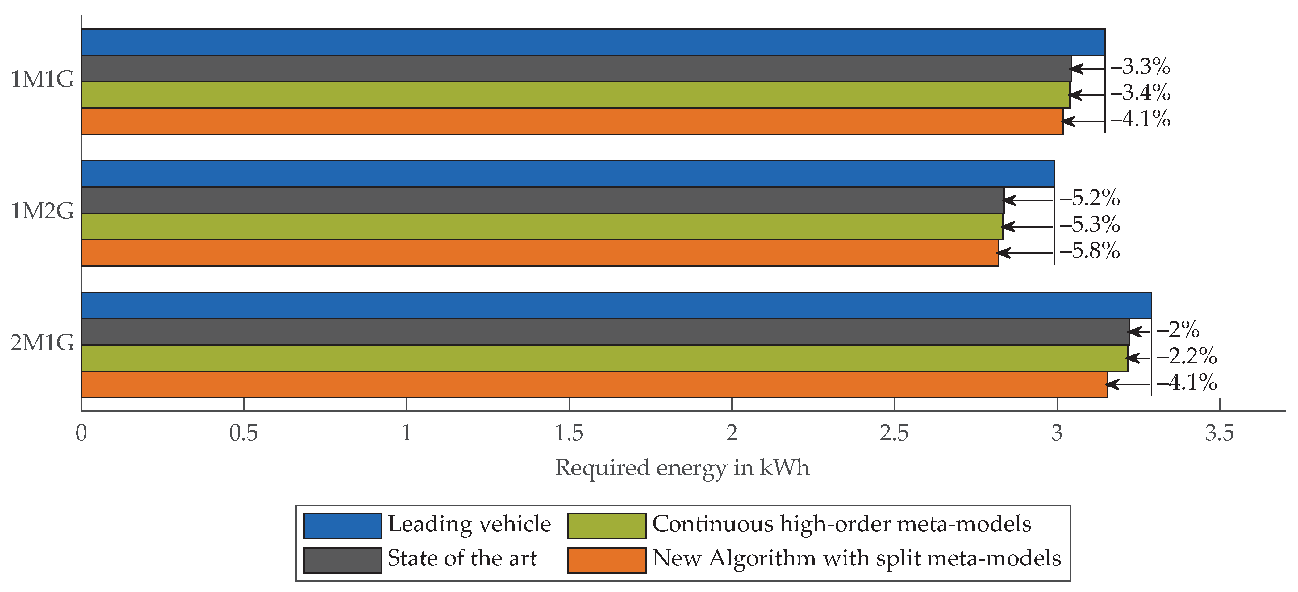
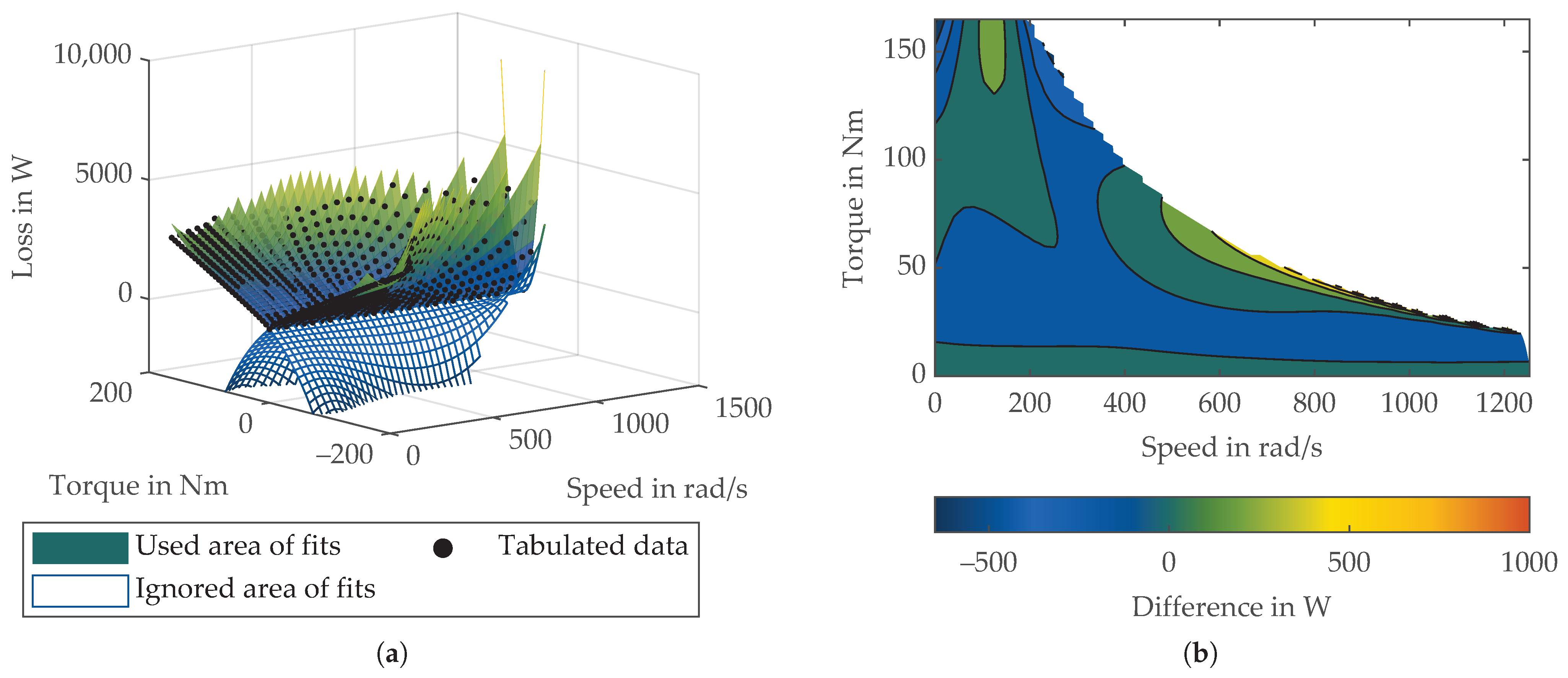
5.2. Comparison to Other Algorithms and Quality Analysis of Meta-Models

As can be seen in Table 1 and Table 3, the fittings of the split meta-models result in significantly lower RMSRE in comparison to the continuous high-order meta-models, even though the polynomial degree of the continuous meta-models is higher. The continuous low-order fitting that represents the state-of-the-art (Table 2) shows the highest RMSRE. The smaller approximation error of the split meta-model can be explained with the concept shown in Figure 2. In contrast to the split meta-models, the continuous fits cannot represent the actual losses, especially around zero torque.

Figure 5 shows the data points of the tabulated model and the resulting fits of the split meta-models for the PMSM. The areas excluded due to the inequality constraints of Equations (36) and (37) are shown without surface color. Due to the two fits, a V-shape can be represented around zero torque. The data points of the tabulated model and the resulting fits of the IM as well as from the transmission of the PMSM are shown in the Appendix. Noteworthy is the different shape of the losses of PMSM and IM, especially at zero torque. The higher RMSRE of the PMSM in contrast to the IM can be explained by the fact that the tabulated data of the PMSM was obtained from measurement data, which itself has a certain scatter.

Figure 6 shows the resulting energy consumption for the car-following scenario for the three different powertrain topologies, using the different meta-models. Furthermore, the energy consumption of the leading vehicle is shown as a reference, whereby the powertrain operation of the 1M2G- and 2M1G-topology was optimized based on our proposed split meta-models.

As can be seen in Figure 6, our proposed algorithm uses the least amount of energy for all powertrain topologies. The relative energy savings with respect to the leading vehicle and with respect to the other algorithms depend on the powertrain topology. Furthermore, it can be seen, that the optimization with continuous high-order polynomial meta-models for motor and gearbox saves almost equally as much energy as the state-of-the-art algorithm based on a continuous low-order polynomial meta-model for the motor and constant gearbox efficiency. This shows the interdependence of the tabulated models and meta-models and the importance of the split meta-model approach. Optimization results are only as good as the underlying powertrain model in combination with their representation within the meta-models. So even though the continuous high-order polynomial meta-models use the implementation of the gearbox loss model and have closer fits due to the higher polynomial degrees, they cannot significantly enhance the energy savings with respect to the state-of-the-art algorithm. This is due to the continuous fits, which fail to represent the V-shape around zero torque. The implementation of the split meta-models results in fits with a smaller approximation error, even though they use lower polynomial degrees than in the continuous high-order meta-models. Thus, this algorithm allows the highest energy savings. Furthermore, it can be seen that 2M1G requires more energy than 1M1G. This is due to the additional weight but also due to the additional load-independent losses. Thus, their modeling of them is crucial for the evaluation of powertrain topologies.

The relative energy-saving potential of the proposed algorithm with respect to the state-of-the-art algorithm depends on the powertrain topology. For the 1M1G-topology, the proposed algorithm saves 25% more energy than the state-of-the-art. For the 2M1G-topology the saving gains rise to 101%. The energy consumption of the 2M1G topology is not only influenced by the vehicle speed profile but also by the internal powertrain operation.

As can be seen in Figure 7a–c, the optimizations with the continuous meta-models use both motors simultaneously to accelerate the vehicle, while the optimization with the split meta-model uses only one motor to propel the vehicle. Thus, the split meta-model finds a more efficient powertrain operation for the 2M1G topology than the continuous meta-models, due to the more accurate representation of the actual losses. Figure 7d–f shows the computed energy consumption based on the tabulated models and meta-models for the 2M1G powertrain topology. It can be seen, that the split meta-models represent the tabulated models, while the calculated energy consumption based on the continuous meta-models differs from the energy consumption based on the tabulated models.

The resulting optimal speed profile for the 1M1G-topology as well as the speed of the leading vehicle and the speed limit are shown in Figure 8.

Figure 9 shows the speed profile as well as the motor air gap torque for the 1M1G-topology in the city-to-city scenario for both the split and continuous high-order polynomial meta-models.

As can be seen from the figure, the optimal speed profile of the split meta-models includes gliding, while the optimal speed profile of the continuous meta-models does not. This can be explained by the better representation of the V-shape of the power loss models by the split meta-models at low torques. This behavior underlines the necessity of the proposed combination of inequality constraints to accurately represent the power and torque losses.

5.3. Computational Analysis

For the car-following scenario, the average solving time on a laptop with an Intel Core i7-7820HQ with 16 GB of RAM is shown in

Table 5. Average solving time of the algorithm for different prediction horizons in the car-following scenario using V2V-prediction. Values in braces belong to the relaxed optimization of the 1M2G-topology.

	1M1G	1M2G	2M1G
Horizon 6 $\mathrm{s}$	$37.2$$\mathrm{m}$$\mathrm{s}$	$52.2$$\mathrm{m}$$\mathrm{s}$ ($44.3$ $\mathrm{m}$$\mathrm{s}$)	58 $\mathrm{m}$$\mathrm{s}$
Horizon 10 $\mathrm{s}$	$59.6$$\mathrm{m}$$\mathrm{s}$	$87.4$$\mathrm{m}$$\mathrm{s}$ ($71.4$ $\mathrm{m}$$\mathrm{s}$)	$91.5$$\mathrm{m}$$\mathrm{s}$
Horizon 16 $\mathrm{s}$	$99.9$$\mathrm{m}$$\mathrm{s}$	$143.4$$\mathrm{m}$$\mathrm{s}$ ($116.6$ $\mathrm{m}$$\mathrm{s}$)	148 $\mathrm{m}$$\mathrm{s}$

.

The average solving time depends on the horizon and powertrain topology. Since the 1M2G-topology needs to solve two optimizations, the solver time of the relaxed problem is presented in braces. With an average solving time of less than one second, the algorithm may be online-capable. However, it should be noted that approaching speed limits, that require the vehicle to reduce speed, are computationally expensive and require more than 1 $\mathrm{s}$. Here, a better implementation of the speed limits may be required. Alternatively, the algorithm could be adapted in the spatial domain; however, with these algorithms, waiting at a standstill is a challenging task to solve.

5.4. Influence of No-Load Losses, and Limitations

The influence of the no-load losses must be considered in a differentiated manner: For an existing vehicle, the mechanical no-load losses at zero torque in the transmission and motor can also be assigned to the wheel-to-distance losses by fitting the coast-down behavior of the vehicle. If no precise analysis is required, it does not matter which component provides resistance to the vehicle. However, this approach leads to problems when additional powertrain components are simulatively integrated into a vehicle, such as a second-driven axle. The second powered axle leads to increased losses, even if the components are only dragged along. Thus, modeling of the mechanical no-load losses at zero torque is required. Since the mechanical no-load losses depend on the rotational speed, the assignment of the no-load losses to wheel-to-distance losses also does not work for two-speed transmissions, since in this case the speed is no longer uniquely linked to the rotational speed of the motor. In addition, there are electrical no-load losses at zero torque. With a PMSM, electrical power is required to make the motor torque-free in the air gap. Since optimal speed profiles of electric vehicles include gliding, these operation points are modeled in this algorithm.

Although the powertrain model described is very detailed, simplifications are still included. The inertia of the powertrain depends on the selected gear. This is neglected in the optimization. Furthermore, the transmission design tool does not allow for an explicit consideration of two-speed transmissions. As a substitute, two transmissions were created, each with one gear of the two-speed transmission. The two loss maps are similar and so only the more conservative loss model is used for both gears. More detailed modeling of the two-speed transmission may improve accuracy in the future.

Due to the available data, validation could only be performed at the overall vehicle level. This means that the overall system can be checked for plausibility, but the individual components cannot be validated. The advantage of the algorithm modeling each component individually has the associated disadvantage that many parameters must be used and the components must also be validated individually. Unfortunately, this was not possible. As a result, the described transmission model cannot be finally validated either. Nevertheless, the results of the overall system are reasonable. Since the motor is based on measurement data, the results of the transmission can be assumed to be plausible. In order to further improve the parameterization of the algorithm in the future, the measurement will have to be taken on the individual components.

The modified powertrain topologies are randomly chosen and do not represent an optimal powertrain. Thus, their performance could be improved by right-sizing the components. This could be achieved by powertrain optimization, as shown in [11,12].

Finally, the chosen scenarios are not representative of all driving scenarios. Regarding the validation, we chose the cycles due to the available real-world measurement data. However, they depict a wide range of driving situations for personal vehicles. The city-to-city scenario is chosen as it was already used in [10] to show differences between different optimization techniques. The car-following scenario is influenced by the idea of Mersky and Samaras [66]. They proposed a car-following scenario for fuel economy testing of autonomous vehicles, to accommodate for the vehicles driving style.

6. Conclusions

In this paper, we have presented a nonlinear programming eco-driving algorithm for different battery electric powertrain topologies which is able to reduce the energy demand in comparison to state-of-the-art eco-driving algorithms. The innovative approaches of this algorithm are

• Incorporated detailed losses, including battery losses, inverter losses, motor losses, transmission losses and driving losses from rolling resistance and air resistance. In contrast to other algorithms, the losses occurring when gliding under no-load are considered more accurate. This becomes important since optimal driving includes gliding.
• A method, to properly fit the losses of the motor and transmission for the optimization by using two polynomials, one for positive torque and the other for negative torque. The two polynomials are interleaved via a help variable and inequality constraints.

The validation experiments show, that the models used can reflect real-world vehicles’ energy consumption in a wide range of driving cycles. Furthermore, the proposed fitting approach allows accurate fits over the whole region of the loss maps. Thereby, the losses are integrated into the optimization with only a small modeling error. The results show, that the chosen meta-model affects the optimal solution. Optimal speed profile and powertrain operation differ in comparison to a continuous fit. The proposed algorithm saves more energy than a state-of-the-art algorithm. Furthermore, we have shown that the new approach of split meta-models is required to reach the highest potential of energy savings, by comparing the results of the split meta-models to continuous high-order polynomial meta-models. We publish the algorithm open-source.

Future work may include a more accurate validation of the single components, the integration of combustion engines and corresponding transmissions for the consideration of hybrid electric vehicles and the integration of the algorithm in real-world applications. An analysis regarding the influence of different scenarios should be conducted in the future, too. Since non-convex optimization can result in local optima, a review of the numerically computed optima qualities should be conducted. Furthermore, a detailed cost analysis is required to make statements about the economics.

References

1. Koenig, A.; Schockenhoff, F.; Koch, A.; Lienkamp, M. Concept Design Optimization of Autonomous and Electric Vehicles. In Proceedings of the 8th International Conference on Power Science and Engineering (ICPSE), Dublin, Ireland, 2–4 December 2019; pp. 44–49. [Google Scholar] [CrossRef]
2. Talebpour, A.; Mahmassani, H.S. Influence of connected and autonomous vehicles on traffic flow stability and throughput. Transp. Res. Part C Emerg. Technol. 2016, 71, 143–163. [Google Scholar] [CrossRef]
3. Stern, R.E.; Cui, S.; Delle Monache, M.L.; Bhadani, R.; Bunting, M.; Churchill, M.; Hamilton, N.; Pohlmann, H.; Wu, F.; Piccoli, B.; et al. Dissipation of stop-and-go waves via control of autonomous vehicles: Field experiments. Transp. Res. Part C Emerg. Technol. 2018, 89, 205–221. [Google Scholar] [CrossRef] [Green Version]
4. Sciarretta, A. Energy-Efficient Driving of Road Vehicles: Toward a Cooperative, Connected, and Automated Mobility; Springer: Cham, Switzerland, 2019. [Google Scholar] [CrossRef]
5. Christian, A. Antriebskonzept-Optimierung für Batterieelektrische Allradfahrzeuge. Ph.D. Thesis, Technische Universität München, Munich, Germany, 2020. [Google Scholar]
6. Vaillant, M. Design Space Exploration zur Multikriteriellen Optimierung Elektrischer Sportwagenantriebsstränge; Karlsruher Institut für Technologie: Karlsruhe, Germany, 2015. [Google Scholar] [CrossRef]
7. Weiß, F. Optimale Konzeptauslegung elektrifizierter Fahrzeugantriebsstränge; Springer: Wiesbaden, Germany, 2018. [Google Scholar] [CrossRef]
8. Verbruggen, F.; Salazar, M.; Pavone, M.; Hofman, T. Joint Design and Control of Electric Vehicle Propulsion Systems. In Proceedings of the 2020 European Control Conference (ECC), St. Petersburg, Russia, 12–15 May 2020; pp. 1725–1731. [Google Scholar] [CrossRef]
9. Wei, C.; Hofman, T.; Ilhan Caarls, E. Co-Design of CVT-Based Electric Vehicles. Energies 2021, 14, 1825. [Google Scholar] [CrossRef]
10. Koch, A.; Bürchner, T.; Herrmann, T.; Lienkamp, M. Eco-Driving for Different Electric Powertrain Topologies Considering Motor Efficiency. World Electr. Veh. J. 2021, 12, 6. [Google Scholar] [CrossRef]
11. Anselma, P.G.; Belingardi, G. Enhancing Energy Saving Opportunities through Rightsizing of a Battery Electric Vehicle Powertrain for Optimal Cooperative Driving. SAE Int. J. Connect. Autom. Veh. 2020, 3. [Google Scholar] [CrossRef]
12. Gambhira, U.R. Powertrain Optimization of an Autonomous Electric Vehicle. Master’s Thesis, The Ohio State University, Columbus, OH, USA, 2018. [Google Scholar]
13. Borsboom, O.; Fahdzyana, C.A.; Hofman, T.; Salazar, M. A Convex Optimization Framework for Minimum Lap Time Design and Control of Electric Race Cars. IEEE Trans. Veh. Technol. 2021, 70, 8478–8489. [Google Scholar] [CrossRef]
14. Huang, Y.; Ng, E.C.Y.; Zhou, J.L.; Surawski, N.C.; Chan, E.F.C.; Hong, G. Eco-driving technology for sustainable road transport: A review. Renew. Sustain. Energy Rev. 2018, 93, 596–609. [Google Scholar] [CrossRef]
15. Fafoutellis, P.; Mantouka, E.G.; Vlahogianni, E.I. Eco-Driving and Its Impacts on Fuel Efficiency: An Overview of Technologies and Data-Driven Methods. Sustainability 2021, 13, 226. [Google Scholar] [CrossRef]
16. Han, J.; Vahidi, A.; Sciarretta, A. Fundamentals of energy efficient driving for combustion engine and electric vehicles: An optimal control perspective. Automatica 2019, 103, 558–572. [Google Scholar] [CrossRef]
17. So, K.M.; Gruber, P.; Tavernini, D.; Karci, A.E.H.; Sorniotti, A.; Motaln, T. On the Optimal Speed Profile for Electric Vehicles. IEEE Access 2020, 8, 78504–78518. [Google Scholar] [CrossRef]
18. Koch, A.; Teichert, O.; Kalt, S.; Ongel, A.; Lienkamp, M. Powertrain Optimization for Electric Buses under Optimal Energy-Efficient Driving. Energies 2020, 13, 6451. [Google Scholar] [CrossRef]
19. Zhang, C.; Vahidi, A. Predictive cruise control with probabilistic constraints for eco driving. In Proceedings of the Dynamic Systems and Control Conference, Arlington, VI, USA, 31 October 31–2 November 2011; Volume 54761, pp. 233–238. [Google Scholar] [CrossRef]
20. Dollar, R.A.; Vahidi, A. Quantifying the impact of limited information and control robustness on connected automated platoons. In Proceedings of the 2017 IEEE 20th International Conference on Intelligent Transportation Systems (ITSC), Yokohama, Japan, 16–19 October 2017; pp. 1–7. [Google Scholar] [CrossRef]
21. Dollar, R.A.; Vahidi, A. Efficient and collision-free anticipative cruise control in randomly mixed strings. IEEE Trans. Intell. Veh. 2018, 3, 439–452. [Google Scholar] [CrossRef]
22. Lin, X.; Görges, D.; Weißmann, A. Simplified Energy-Efficient Adaptive Cruise Control based on Model Predictive Control. IFAC-PapersOnLine 2017, 50, 4794–4799. [Google Scholar] [CrossRef]
23. Diehl, M.; Bock, H.G.; Diedam, H.; Wieber, P.B. Fast direct multiple shooting algorithms for optimal robot control. In Fast Motions in Biomechanics and Robotics; Springer: Berlin/Heidelberg, Germany, 2006; pp. 65–93. [Google Scholar]
24. Rao, A. A Survey of Numerical Methods for Optimal Control. Adv. Astronaut. Sci. 2010, 135. Available online: https://www.researchgate.net/publication/268042868_A_Survey_of_Numerical_Methods_for_Optimal_Control (accessed on 6 July 2022).
25. Lin, X.; Gorges, D.; Liu, S. Eco-driving assistance system for electric vehicles based on speed profile optimization. In Proceedings of the 2014 IEEE Conference on Control Applications (CCA), Juan Les Antibes, France, 8–10 October 2014; pp. 629–634. [Google Scholar] [CrossRef]
26. Lajunen, A. Energy-optimal velocity profiles for electric city buses. In Proceedings of the 2013 IEEE International Conference on Automation Science and Engineering (CASE), Madison, WI, USA, 17–20 August 2013; pp. 886–891. [Google Scholar] [CrossRef]
27. Franke, R.; Terwiesch, P.; Meyer, M. An algorithm for the optimal control of the driving of trains. In Proceedings of the 39th IEEE Conference on Decision and Control (Cat. No.00CH37187), Sydney, NSW, Australia, 12–15 December 2000; pp. 2123–2128. [Google Scholar] [CrossRef]
28. Liao, P.; Tang, T.Q.; Liu, R.; Huang, H.J. An eco-driving strategy for electric vehicle based on the powertrain. Appl. Energy 2021, 302, 117583. [Google Scholar] [CrossRef]
29. Shao, Y. Optimization and Evaluation Of Vehicle Dynamics and Powertrain Operation For Connected and Autonomous Vehicles. Ph.D. Thesis, University of Minnesota Digital Conservancy, Minneapolis, MN, USA, 2019. [Google Scholar]
30. Wächter, A.; Biegler, L.T. On the implementation of an interior-point filter line-search algorithm for large-scale nonlinear programming. Math. Program. 2006, 106, 25–57. [Google Scholar] [CrossRef]
31. Jia, Y.; Jibrin, R.; Gorges, D. Energy-Optimal Adaptive Cruise Control for Electric Vehicles Based on Linear and Nonlinear Model Predictive Control. IEEE Trans. Veh. Technol. 2020, 69, 14173–14187. [Google Scholar] [CrossRef]
32. Bertoni, L.; Guanetti, J.; Basso, M.; Masoero, M.; Cetinkunt, S.; Borrelli, F. An adaptive cruise control for connected energy-saving electric vehicles. IFAC-PapersOnLine 2017, 50, 2359–2364. [Google Scholar] [CrossRef]
33. Hucho, W.H. Aerodynamics of road vehicles. SAE Int. 1986, 295–354. [Google Scholar] [CrossRef]
34. Schwickart, T.; Voos, H.; Hadji-Minaglou, J.R.; Darouach, M.; Rosich, A. Design and simulation of a real-time implementable energy-efficient model-predictive cruise controller for electric vehicles. J. Frankl. Inst. 2015, 352, 603–625. [Google Scholar] [CrossRef]
35. He, H.; Liu, D.; Lu, X.; Xu, J. ECO Driving Control for Intelligent Electric Vehicle with Real-Time Energy. Electronics 2021, 10, 2613. [Google Scholar] [CrossRef]
36. Guzzella, L.; Sciarretta, A. Vehicle Propulsion Systems: Introduction to Modeling and Optimization, 3rd ed.; Springer: Berlin/Heidelberg, Germany, 2013. [Google Scholar] [CrossRef]
37. Braess, H.H.; Seiffert, U. (Eds.) Vieweg Handbuch Kraftfahrzeugtechnik, 7 aktualisierte auflage ed.; ATZ/MTZ-Fachbuch; Springer: Wiesbaden, Germany, 2013. [Google Scholar] [CrossRef]
38. Highway Tire Committee. Stepwise Coastdown Methodology for Measuring Tire Rolling Resistance. [CrossRef]
39. Hall, D.E.; Moreland, J.C. Fundamentals of Rolling Resistance. Rubber Chem. Technol. 2001, 74, 525–539. [Google Scholar] [CrossRef]
40. Ficht, A.; Lienkamp, M. Rolling resistance modeling for electric vehicle consumption. In 6th International Munich Chassis Symposium 2015; Pfeffer, P., Ed.; Springer: Wiesbaden, Germany, 2015; pp. 775–798. [Google Scholar] [CrossRef]
41. Ejsmont, J.; Taryma, S.; Ronowski, G.; Swieczko-Zurek, B. Influence of temperature on the tyre rolling resistance. Int. J. Automot. Technol. 2018, 19, 45–54. [Google Scholar] [CrossRef]
42. Mitschke, M.; Wallentowitz, H. Dynamik der Kraftfahrzeuge; Springer: Wiesbaden, Germany, 2014. [Google Scholar] [CrossRef]
43. Steinstraeter, M.; Heinrich, T.; Lienkamp, M. Effect of Low Temperature on Electric Vehicle Range. World Electr. Veh. J. 2021, 12, 115. [Google Scholar] [CrossRef]
44. Fotouhi, A.; Auger, D.J.; Propp, K.; Longo, S.; Wild, M. A review on electric vehicle battery modelling: From Lithium-ion toward Lithium–Sulphur. Renew. Sustain. Energy Rev. 2016, 56, 1008–1021. [Google Scholar] [CrossRef] [Green Version]
45. Chang, F.; Ilina, O.; Lienkamp, M.; Voss, L. Improving the Overall Efficiency of Automotive Inverters Using a Multilevel Converter Composed of Low Voltage Si mosfets. IEEE Trans. Power Electron. 2019, 34, 3586–3602. [Google Scholar] [CrossRef]
46. Xu, Y.; Gu, J.; Chen, H.; Chen, Z.; Pu, Y. Power loss calculation for the power converter in switched reluctance motor drive. In Proceedings of the 2014 IEEE International Conference on Information and Automation (ICIA), Hailar, China, 28–30 July 2014; pp. 19–24. [Google Scholar] [CrossRef]
47. Jenni, F.; Wüest, D. Steuerverfahren für selbstgeführte Stromrichter; Verlag an der ETH Zürich: Zürich, Switzerland, 1995. [Google Scholar] [CrossRef]
48. Binder, A. Elektrische Maschinen und Antriebe; Springer: Berlin/Heidelberg, Germany, 2017. [Google Scholar] [CrossRef]
49. Müller, G.; Ponick, B. Grundlagen Elektrischer Maschinen, 10 wesentlich überarbeitete und erweiterte auflage ed.; Elektrische Maschinen/Germar Müller und Bernd Ponick; Wiley-VCH Verlag GmbH & Co. KGaA: Weinheim, Germany, 2014; Volume 1. [Google Scholar]
50. Mahmoudi, A.; Soong, W.L.; Pellegrino, G.; Armando, E. Loss Function Modeling of Efficiency Maps of Electrical Machines. IEEE Trans. Ind. Appl. 2017, 53, 4221–4231. [Google Scholar] [CrossRef] [Green Version]
51. Ruuskanen, V.; Nerg, J.; Rilla, M.; Pyrhonen, J. Iron Loss Analysis of the Permanent-Magnet Synchronous Machine Based on Finite-Element Analysis Over the Electrical Vehicle Drive Cycle. IEEE Trans. Ind. Electron. 2016, 63, 4129–4136. [Google Scholar] [CrossRef]
52. Niemann, G.; Winter, H. Maschinenelemente: Band 2: Getriebe Allgemein, Zahnradgetriebe—Grundlagen, Stirnradgetriebe; Niemann, G., Winter, H., Eds.; Springer: Berlin/Heidelberg, Gernmany, 2003. [Google Scholar]
53. Pahl, G.; Müller, H.W. Die Umlaufgetriebe; Springer: Berlin/Heidelberg, Germany, 1998; Volume 28. [Google Scholar] [CrossRef]
54. Walter, P. Anwendungsgrenzen für die Tauchschmierung von Zahnradgetrieben, Plansch- und Quetschverluste bei Tauchschmierung: Forschungsvorhaben Nr. 44/I; Abschlußbericht; Forschungsvereinigung Antriebstechnik: Forschungsheft, Germany, 1982. [Google Scholar]
55. SKF. Rolling Bearings|SKF. 2021. Available online: https://www.skf.com/group/products/rolling-bearings (accessed on 15 November 2021).
56. Schaeffler Technologies AG & Co. KG. Rolling Bearings: Ball bearings, Roller Bearings, Needle Roller Bearings, Track Rollers, Bearings for Screw Drives, Insert Bearings/Housing Units, Bearing Housings, Accessories. 2019. Available online: https://www.schaeffler.de/content.schaeffler.de/de/news_medien/mediathek/publikationen/downloadcenter-global-pages/downloadcenter-language-list-publications.jsp?pubid=246581&ppubid=246579&tab=mediathek-pub&uid=386195&subfilter=app:dc (accessed on 6 February 2021).
57. Wolf, T.M. The Rolling Bearing in the Electrified Power Train—Requirements and Solutions. In CTI SYMPOSIUM 2019; Springer: Berlin/Heidelberg, Gernmany, 2021; pp. 575–583. [Google Scholar] [CrossRef]
58. ISO 14179. Gears—Thermal Capacity—Part 2: Thermal Load-Carrying Capacity. International Organization for Standardization: Geneva, Switzerland, 2001. [Google Scholar]
59. Marler, R.T.; Arora, J.S. The weighted sum method for multi-objective optimization: New insights. Struct. Multidiscip. Optim. 2010, 41, 853–862. [Google Scholar] [CrossRef]
60. Andersson, J.A.E.; Gillis, J.; Horn, G.; Rawlings, J.B.; Diehl, M. CasADi—A software framework for nonlinear optimization and optimal control. Math. Program. Comput. 2019, 11, 1–36. [Google Scholar] [CrossRef]
61. Wassiliadis, N.; Steinsträter, M.; Schreiber, M.; Rosner, P.; Nicoletti, L.; Schmid, F.; Ank, M.; Teichert, O.; Wildfeuer, L.; Schneider, J.; et al. Quantifying the state of the art of electric powertrains in battery electric vehicles: Range, efficiency, and lifetime from component to system level of the Volkswagen ID.3. eTransportation 2022, 12, 100167. [Google Scholar] [CrossRef]
62. Paar, C.; Muetze, A.; Kolbe, H. Influence of Machine Integration on the Thermal Behavior of a PM Drive for Hybrid Electric Traction. IEEE Trans. Ind. Appl. 2015, 51, 3914–3922. [Google Scholar] [CrossRef]
63. Kiyota, K.; Kakishima, T.; Chiba, A. Estimation and comparison of the windage loss of a 60 kW Switched Reluctance Motor for hybrid electric vehicles. In Proceedings of the 2014 International Power Electronics Conference (IPEC-Hiroshima 2014—ECCE ASIA), Hiroshima, Japan, 18–21 May 2014; pp. 3513–3518. [Google Scholar] [CrossRef]
64. Nicoletti, L.; Köhler, P.; König, A.; Heinrich, M.; Lienkamp, M. Parametric Modeling of Weight and Volume Effects on Battery Electric Vehicles, with Focus on the Gearbox. Proc. Des. Soc. 2021, 1, 2389–2398. [Google Scholar] [CrossRef]
65. Kalt, S.; Erhard, J.; Lienkamp, M. Electric Machine Design Tool for Permanent Magnet Synchronous Machines and Induction Machines. Machines 2020, 8, 15. [Google Scholar] [CrossRef] [Green Version]
66. Mersky, A.C.; Samaras, C. Fuel economy testing of autonomous vehicles. Transp. Res. Part C Emerg. Technol. 2016, 65, 31–48. [Google Scholar] [CrossRef]
Figure 1. Power flow in the electric powertrain and the losses considered in the optimization in red.
Energies 15 05396 g001
Figure 2. Fitting concepts for losses with V-shape. Continuous fits fail to fit the point around zero torque, even for high polynomial degrees.
Energies 15 05396 g002
Figure 3. Overview of the parameterization, optimization and simulation process. A detailed comparison between vehicle measurements and calculated energy consumption as well as a comparison between the tabulated models and meta-models are presented in Section 5.1 and Section 5.2, respectively.
Energies 15 05396 g003
Figure 4. Battery output energy consumption of measurement data [61] and simulation for the 2nd run of the WLTP, urban, intercity, and highway-cycle.
Energies 15 05396 g004
Figure 5. (a) Electrical motor losses of ID.3: fits of the split meta-model and the corresponding data points of the tabulated model. The ranges used due to the inequality constraints of Equations (36) and (37) are highlighted with the surface color. Irrelevant ranges of fits are presented with grid lines only. (b) Difference between fit and tabulated electrical motor losses.
Energies 15 05396 g005
Figure 6. Energy consumption of the leading vehicle and the ego vehicle using different types of eco-driving algorithms.
Energies 15 05396 g006
Figure 7. (ac): Torque division between the two motors of the 2M1G topology based on the split meta-models, continuous high-order meta-models and continuous low-order meta-models. (df): Energy consumption of simulation (tabulated models) and optimization (meta-models) for the 2M1G-topology.
Energies 15 05396 g007
Figure 8. Speed profiles of car-following vehicle and leading vehicle as well as the speed limit.
Energies 15 05396 g008
Figure 9. Comparison of (a) speed profiles and (b) corresponding motor torque during the city-to-city-scenario for split and continuous high-order meta-models.
Energies 15 05396 g009