1. Introduction
Reaching net zero CO
2 emissions requires rapid decarbonisation of the built environment [
1]. Globally, over half of buildings are heated using direct combustion of fossil fuels [
2], but decarbonisation of heating is widely expected to require switching to heat pumps powered by renewable or other low carbon electricity [
3]. The electrification of heat will create new challenges for local and national electricity systems, such as local grid congestion [
4] and large seasonal variation in electricity demand [
5] alongside increased electricity demands from the electrification of the transport sector [
6]. These challenges have led to much work on how demand-side flexibility may be used to decrease and diversify the peak electricity demand [
7].
The UK has a stock of 28 million dwellings, with approximately 24 million gas boilers and 2 million oil boilers [
8] to replace with low carbon alternatives. The energy performance of UK homes, with their respective energy conversion technologies, is indicated through Energy Performance Certificate (EPC) ratings, which are also used to provide recommendations to householders and landlords on cost-effective energy related upgrades. EPC ratings in the UK are derived from closely related methods to those used in many territories: physical survey of properties, followed by modelling which estimates the annual energy costs from a standard usage pattern [
9]. As the energy system decarbonises and the requirements placed upon it change through the electrification of heat and transport, the information provided by EPCs may need to change to better reflect the costs to consumers and to recommend appropriate retrofit measures. One type of information of emerging importance is around peak electrical power demand and ability to shift it out of periods of electricity system stress [
10]. This ability is termed flexibility and enables households to participate in demand side response (DSR).
The concept of rating buildings using metrics associated with flexibility has a growing presence in the literature. Different parameterisations of flexibility can be used to reflect the different actors and perspectives across the energy system [
7,
11]; for example, a focus on energy supply may value the size of load which can be shed, while the building user may value the internal temperature remaining as constant as possible through a load-shedding or load-absorbing event. The vast majority of studies use building simulation methods to quantify flexibility potential and/or derive flexibility ratings. This ensures that different buildings can be modelled under the same weather conditions and electricity system requests (e.g., preventing curtailment or system damage by absorbing excess electricity, or shifting electricity use from a peak) and also allows stock models of flexibility to be created [
12,
13]. However, these models are not validated empirically [
13]. Reference [
14] showed that it is possible to calibrate a simulation model to predict the real internal temperature swings associated with flexible heat pump operation for a single building, but this takes considerable time and real data.
Meanwhile, in a number of countries there has been recent research effort and governmental backing for empirical building performance ratings [
15,
16]. Acknowledging some of the issues with theoretical (asset) ratings such as assessor variability [
17,
18], lack of incentive for retrofit work to be of a high quality and lack of public trust [
19], measured energy data can be used to derive metrics spanning from operational energy use (energy use per unit floor area under standardised weather conditions) to the heat transfer coefficient (a physical characteristic of the building fabric). In previous work we discussed how such metrics may now be calculated on a large scale due to the availability of smart meter data [
10].
This paper introduces an empirical flexibility metric which can be used to inform consumers, aggregators and other actors about the potential of different properties to avoid space heating during critical peak periods. The empirical flexibility metric is conceptually and practically very different to existing flexibility rating methods and this work aims to inform the debate on how such empirical methods may give insights into building flexibility potential. This paper introduces a simple, informative metric, intended to be further developed and combined with other approaches to describing flexibility and DSR potential.
The next section of this paper introduces buildings and energy flexibility, describes the physical processes occurring when buildings are subjected to changes in heating input and which underpin changes in internal temperature.
Section 3 describes the dataset and method used to create the empirical flexibility metric; steps in the method are validated and implemented across the whole dataset in
Section 4.
Section 5 discusses the uses for the metric, its limitations and how such methods may be developed, and
Section 6 summarises the paper.
2. Theory
2.1. Aim of the Flexibility Metric
The aim of the empirical flexibility metric, as discussed in this work, is to provide householders and actors who may provide services to them (such as aggregators) with an indication of the building’s ability to be operated flexibly with a decarbonised heating system, even if they do not yet have the technology to do this (e.g., a heat pump). This aim requires consideration of what is meant by operating flexibly and how the suitability of the building can be assessed.
2.1.1. Valuing Flexibility
Energy flexibility, as discussed above, is valuable to different parts of the electricity system in different circumstances [
20]. This article is written from a perspective in which the value of flexibility is in adding the lowest possible electricity demand to the electricity system during peak demand periods. The characteristics of the largest peaks in energy demand vary by country, but in Britain it currently consists of a 2–4 h period commencing in the early evening on winter weekdays [
21]. Under widespread adoption of heat pumps, the timing of this peak is likely to remain fairly similar [
22] and there may be a new peak lasting around 2 h in the morning [
5].
The above perspective on the value of flexibility differs from alternatives such as valuing the size of load which can be curtailed from one building, or the quantification of flexibility in [
11] which integrates the size of the load reduction/increase with the time it can be sustained. Such different measures of flexibility highlight the different system services that storage and DSR are expected to provide. In this article, we focus on minimising additional demand during an existing peak period as highly relevant to the provision of information to householders and their service providers, such as through UK EPCs, because:
Unlike a metric which values size of curtailed load, it does not incentivise the use of electric heating systems in leaky buildings, thus corresponding with the energy efficiency emphasis of much energy policy, encapsulated, for example, in the design of EPCs;
Unlike a metric which values the duration of the DSR period, it focusses on the management of demand during typical daily operation, with a peak during a finite time window, whereby flexibility during this window is more valuable than flexibility maintained afterwards.
Under this perspective of providing value to the energy system, maximum flexibility occurs when the heating can be switched off for the entire duration of the defined peak period, thus adding no demand to the electricity system.
2.1.2. Rating the Building
We also require a metric which does not require inputting the capacity and other technical characteristics of a heat pump or other electric heating technology, since the metric is intended to provide an estimate of flexibility in homes which do not necessarily have electrified heating yet. Similar to the empirical heat transfer coefficient (HTC) [
23], the focus is assessment of an individual dwelling on its real in-use performance—in this case its ability to retain thermal energy when heat supply is interrupted for a finite period, likely to be a critical peak period. The thermal energy stored within a property, combined with its rate of heat loss, is central to its ability to be operated flexibly without supplementary energy storage as excessive drops in internal temperature are likely to affect thermal comfort of occupants and may result in the heating being turned back on, customer dissatisfaction, or both, if time of use tariffs penalise such responses. This paper therefore investigates the temperature decay when heating is switched off as a simple and easily measured metric that reflects the potential for the house to be operated in a manner that minimises on-peak demand.
2.2. Physics of Temperature Changes in Buildings
This section focuses on the physical mechanisms occurring when a building drops in temperature after the heating is switched off, followed by a discussion of how to create a metric describing this temperature decay.
2.2.1. Physical Mechanisms of Temperature Decay
The rate at which a building cools down after a period of heating is determined by a combination of building characteristics and other factors. The former are the heat loss coefficient of the building including natural ventilation, thermal mass, and any mechanical ventilation; and the latter comprise the temperature differences between the inside and outside air, ground or adjoining buildings, heat gains originating from sources other than the heating system, and the wind speed [
24].
Heat input from a heating system and other sources is stored in several elements within the building: the structure, the internal contents (e.g., furniture, floor coverings [
25]), the heating system [
26] and the air. All these elements provide thermal mass in different quantities, from the most thermally lightweight (the air) to the most heavyweight (the building structure). At the point that heating is switched off, the different elements are also likely to be at different temperatures. Firstly, the heating system is likely to be warmer than the other thermal masses. Secondly, depending on the length of the preceding heating period and the material characteristics of the different thermal masses present, not all of the thermal mass in the building may have been activated [
27]. This partial activation of the entire thermal mass is quantified using the concept of effective thermal inertia [
25], and results in lighter elements such as the air and lightweight internal contents being warmer than heavier internal structures when the timescales of heating do not enable all the thermal mass to be brought to a homogeneous internal temperature. Thirdly, building elements in contact with external air are cooler than internal air [
28].
Since objects of different temperatures exchange heat, from the time the heating is switched off heat transfer occurs both between the inside and the outside of the dwelling and from the warmer internal elements to the cooler ones. These different heat transfers occur at different rates, with more rapid cooling associated with smaller thermal masses/resistances and larger temperature differences. Two examples of heat transfer during cooling down of a home are as follows. Firstly, a radiator heating system may lose its heat to the air over the first half hour after the heating is turned off [
29], which will slow the rate of cooling of the air during this initial period, or even result in a rise in air temperature in some cases. Secondly, heat is transferred though building elements shared with adjacent properties and depends on the temperature difference across these party elements, which is constantly changing. Party element gains and losses can be important contributors to the total heating demand for a property and due to the large thermal resistances involved this mechanism will occur over longer timescales than the first example.
The result of the highly complex and dynamic heat flows for a property is a change in internal temperature. This can be assessed in one or multiple locations within the property.
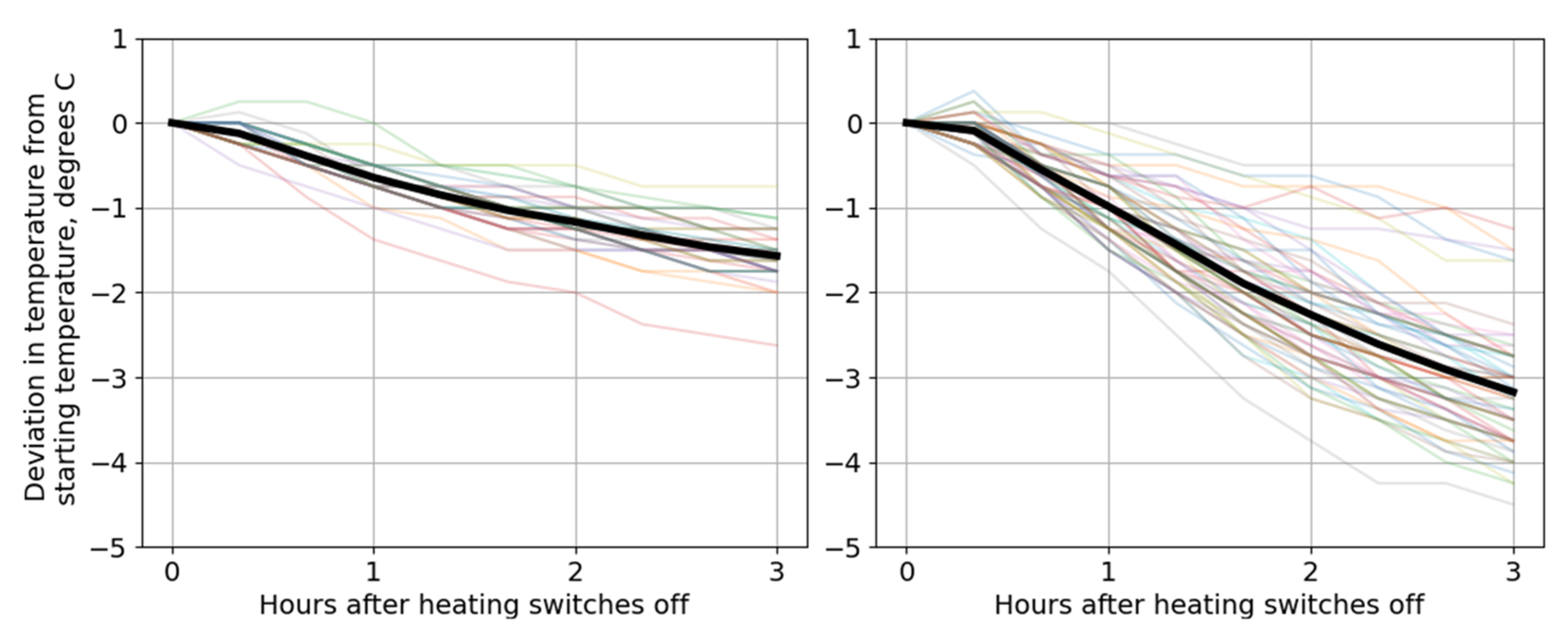
Figure 1 illustrates this for two homes from a publicly available UK dataset known as LEEDR (see
Section 3 for description of the data) [
30]. The figure shows the first three hours of cooling down of the living room only in two examples, a semi detached house with insulated cavity walls (left) and a detached house with uninsulated solid walls (right), after the heating is last switched off in the evening. The occurrence of heating switching off was inferred by observing the last daily occurrence of gas use accompanied by elevated internal temperature, for each day between November and February in which this was visible and for which data was present. Each line in
Figure 1 represents the trajectory in temperature from its starting value for a single day, with the solid black line showing the mean across all days. The starting temperature and outdoor temperatures each day are different.
Both plots in
Figure 1 show that on average, internal temperature drops slowly over the first 20 min, and then more quickly, gradually flattening off. The coloured lines depicting individual days also indicate that it is possible for the temperature to rise in the first 20 min after the heating switches off.
2.2.2. Characterisation of Building Cool Down
At its simplest, the characterisation of cooling down can be simplified to one parameter, the building thermal time constant. This concept is derived from Newton’s law of cooling and assumes that the dwelling and its contents cool down together as one thermal mass with respect to an external heat sink, resulting in an exponential temperature decay. The thermal time constant can be derived from internal temperature data from a single temperature sensor, or by aggregating data from many sensors. The building time constant approach was used by [
31] to characterise a building (although not for the purposes of flexibility), with a single thermal mass model justified by discarding the first hour of data after the heating ended, assuming that the heating system was still transferring energy to the dwelling during this hour. However, the authors presented no temperature data to demonstrate the validity of the one thermal mass model, which can be compromised by internal gains and party element heat transfer, in addition to the different rates of cooling of different thermal masses as described above.
Other authors such as [
13] argue that the use of multiple thermal masses is more appropriate than a single one when modelling building demand response. In Sperber et al.’s work, the optimum model was found to vary with the building and heating type, since in some cases the thermal energy stored in the heating system thermal mass was a significant driver of rate of change of temperature in the first hours of the demand response period. However, this finding was not validated with real temperature data; it was validated using a detailed simulation model. In a real dwelling, characterisation using multiple thermal masses would require multiple temperature sensors measuring not only air but heating system and other thermal mass temperatures; this is likely not realisable over a large number of dwellings.
Outside of a demand response context, Ref. [
32] used Bayesian model comparison to show that the lumped thermal mass models that best represent dynamic performance of a building change according to the time of year and building type. This result was ascertained using temperature data from a number of sensors within the dwelling, with each temperature either representing one thermal mass in order that the model was not underspecified, or being aggregated to represent a larger thermal mass. This research highlights that the physical characterisation of how a building cools down after being heated is complex due to multiple thermal masses acting on different timescales. The applicability of different physical models may be driven by availability of data to avoid under specification of a model preventing parameter identification. In particular, representing the heat transfer from the heating system into the air and fabric requires either accurate temperature data from within that system combined with appropriate modelling, or requires that the temperature of the heating system has dropped to the ambient temperature in the property, avoiding the impact of such heat flows.
2.3. Metric for Flexibility
An empirical measure for flexibility services associated with the building fabric that is suitable for widespread adoption needs to be simple to interpret and to be delivered at low cost. Leveraging data collected for complementary purposes decreases the direct cost of producing flexibility ratings, whilst also adding to the value derived from previous data collection investments. A widespread and low-cost source of energy data is from smart meters, where electricity and gas data are collected at 30-min intervals in the UK and at similar time resolution in other countries. The in-use thermal characterisation methods discussed in
Section 1 use this data, usually with the addition of internal temperature measurement [
23]. The flexibility metric developed in this work therefore adopts the same data requirements: smart meter data and internal temperature.
The challenge of accurately characterising physical processes within the complex and dynamic case of occupied homes is avoided by adopting a metric that does not describe these processes in detail. We instead present one potential simple and easily interpreted measure for the thermal flexibility of the fabric of homes using the measured outcome of the physical processes to characterise how a building cools down: the drop in internal temperature over a defined period after the heating is switched off under standardised conditions.
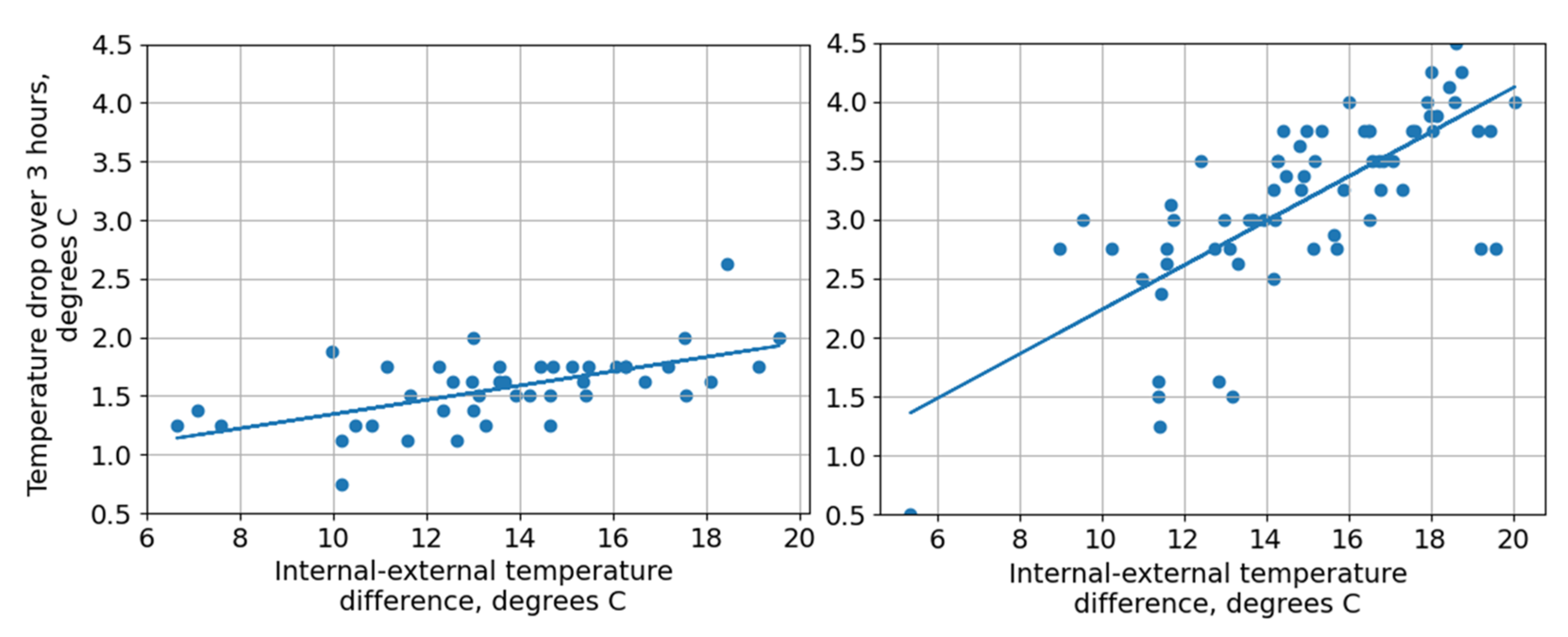
The drop in air temperature over a three-hour period after the heating is switched off is shown in
Figure 2 for the same homes and data as used in
Figure 1.
Figure 2 shows that the rate of temperature decay varies in each home, and that part of this variation is explained by the difference between internal and external temperature. This temperature difference is widely accepted as the main driving force of heat loss from the home to the environment in accordance with the second law of thermodynamics. The correlation coefficient on the left hand and right-hand plots are 0.60 and 0.72 respectively.
To create a useful comparative measure, the temperature drop must be calculated over a consistent duration and at a set internal-external temperature difference. Further, to account for the part of the variation not explained by the temperature difference alone the uncertainty should be stated with the result, such as that given by the 95% confidence interval. For example, using the two houses in
Figure 1 and
Figure 2, at 12 °C internal-external temperature difference, House 05 (left) drops 1.5 ± 0.2 °C, and house 39 (right) drops 2.6 ± 0.4 °C over a three-hour period. The choice of a three-hour period reflects a typical UK evening peak demand duration but any other length of cooling down time can also be used for this type of metric.
3. Methods
3.1. Data
The core data requirements for the method for calculating empirical flexibility metrics are discussed in
Section 2.3: half hourly measurements of internal temperatures, and half hourly gas and electricity use from a smart meter. This paper uses two data sources: data from a small study for method development and data from a larger study to investigate automation and performance over a larger number of homes.
Initial exploratory work was carried out using the publicly available
LEEDR dataset collected and curated by Loughborough University [
30], available since 2018 and containing one minutely (minute-by minute) data on internal temperature (measured in the living room) and gas consumption from 20 properties in the Midlands, England. Method development and testing was carried out using the publicly available
IDEAL Household Energy Dataset, collected and curated by the University of Edinburgh [
33]. This data has only been available since 2021, hence early exploratory work was done using the LEEDR data instead.
The IDEAL dataset includes 255 homes in 5 areas in/around Edinburgh in Scotland, all heated by gas boilers, reflecting the dominant heating system in Great Britain. The dataset contains these measurements at 12-s resolution; these can be aggregated to half hourly values to represent the data that smart metering would provide. Furthermore, the IDEAL dataset contains additional variables useful for the metric development such as central heating flow temperature (see
Section 3.2) at 12-s resolution. This high resolution data can be used to validate and calculate the error on predictions made from the half hourly aggregated data.
A limitation of the IDEAL dataset for developing, testing and interpreting empirical flexibility metrics is the lack of metadata related to the building construction. The relationship between physical attributes of properties determined from a survey, such as their approximate thermal mass, surface to volume ratio and insulation levels, in addition to any modelled performance, and the flexibility metric cannot be explored here and is further discussed in
Section 5.3 and
Section 6.
3.2. Method Development
To create the temperature drop metric in order to rate the flexibility of a large number of homes using half hourly smart meter and temperature data, two steps are necessary. The first is to accurately and automatically determine the time at which the heating switches off on a given day in a home, and the second requires calculating the temperature drop over a predetermined period from that time.
Determination of heating operation from half hourly smart meter data is difficult due to the multiple uses of gas: for space heating throughout a property using a boiler, in individual rooms using gas fires, for hot water and cooking. Heating operation has been predicted from one minutely data [
34] and ten minutely data [
35] using time series analysis and pattern recognition methods but to the authors’ knowledge no published algorithm uses the much sparser half hourly data from smart meters. Thus, a heating operation algorithm was developed and is described in
Section 3.2.1.
3.2.1. Method Step 1: Developing an Algorithm to Predict Heating Operation from Half Hourly Data
The proposed heating operation algorithm combines gas and internal temperature data. It is therefore assumed that the use of gas for space heating corresponds with an increase in dwelling internal temperature, either immediately or with a time offset (further discussed in
Section 3.2.2). This algorithm is therefore physically informed, rather than using a purely statistical approach.
The algorithm is designed to work with half hourly smart meter data, thus at this point we outline what this data is formed of. In gas smart meter data, the data point recorded at a given half hour (e.g., 22:00) is the sum of gas use over the previous thirty minutes (21:30:01–22:00). Temperature data from a standard logger may either record a spot (“instantaneous”) measurement associated with the time stamp, or an average over a given time interval (often equal to the recording interval) taken from multiple measurements. Thus, gas use and temperature changes may not be reported at exactly the instant they occur, instead representing a half hour period.
The space heating status is assigned to on or off (1 or 0 within a vector of length 48 per day) according to the following assumptions:
If gas use is positive and rate of change of temperature is positive, then space heating is on
If gas use is positive and rate of change of temperature is not positive, then space heating is off (and hot water or a gas cooking facility is on)
If gas use is zero, then space heating is off (and all other uses of gas are off).
Whilst the first assumption is provisional on cooking not leading to a rise in internal temperature, such an event is the equivalent of space heating (albeit unintended) for the application discussed in this paper: the derivation of a flexibility metric based on cooling in the absence of heating.
3.2.2. Method Step 2: Calculating the Temperature Drop Metric for Each Dwelling
The output of the heating operation algorithm was used to identify periods of data after the heating was turned off for a given dwelling, to calculate the fall in internal temperature during each such period, and to combine the results into one final value of the temperature drop metric for each dwelling.
For this work, temperature drops occurring overnight were deemed more representative of space heating flexibility potential than those during the day. This is in order to exclude solar gains and to minimise other free heat gains from appliances, occupants and supplementary electric heating. Thus, the final heating off event per night was selected, searching within the period 18:00–02:00. Once the final heating off time was determined for a given night and dwelling, the three following hours were used to calculate the fall in internal temperature. A three hour period was selected since this is likely to represent the typical length of a demand response period during an evening electricity peak [
22]. However, a different period can be selected as required to assess the potential of properties to respond to different demand response events in support of system operation. The internal temperature was allowed to increase for the initial half hour following the heating being switched off, but was required to fall each timestep thereafter in order that the three hour period was deemed valid for use.
For each night in which a valid nightly temperature drop was obtained, this was recorded along with the starting internal temperature and average outdoor temperature over the three-hour period. This was carried out for all nights occurring in winter months (November, December, January, February) capturing cooling over a range of outdoor temperatures. A linear relationship was then used to relate the nightly temperature drop to the inside-outside temperature difference.
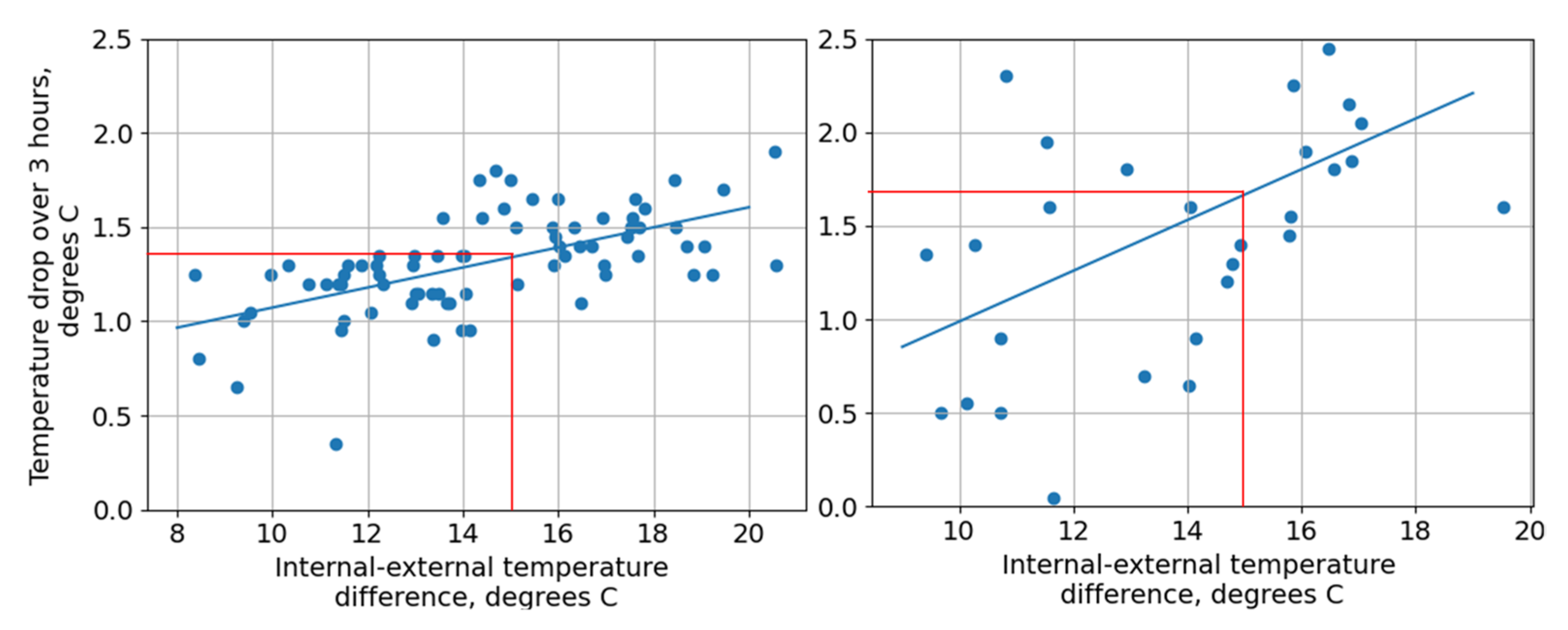
Figure 3 shows the identification of the overnight temperature drop metric from a set of nightly temperature drops from two example homes in the IDEAL dataset—one with a low uncertainty on the line of best fit, the second with high uncertainty. The temperature drop metric was calculated from the derived linear relationship as the overnight temperature drop at a given internal-external temperature difference. In this work an internal-external temperature difference of 15 °C was selected, being approximately in the middle of the temperature difference range measured in the majority of studied homes and reflecting the temperature difference between a starting internal temperature of 20 °C and an external temperature of 5 °C, in line with the November-February UK average rounded to the nearest degree. A different internal-external temperature difference can be selected according to technical, economic or policy criteria.
4. Results
4.1. Heating Operation Algorithm Validation
High resolution (12 s) central heating flow temperature data from the IDEAL dataset was used to validate the heating operation algorithm’s predictions of the final time the heating switched off each night. A random sample of 2 days from each of 60 homes in the IDEAL dataset was selected for validation. The high-resolution flow temperature data was visually inspected to identify firstly whether there was at least one heating-off event from 18:00–02:00, and secondly at what time the final event occurred. It was usually straightforward to visually identify exactly when heating turned on and off from this data, since this corresponded to a sudden and prolonged drop in flow temperature. However, test cases in which it was not clear whether the heating was on or off were discarded, leaving 94 test cases labelled with a ground truth consisting either of ‘no heating-off event’ or the time of the final heating-off event.
The heating operation algorithm described in
Section 3.2.1 was tested on half hourly gas and internal temperature data from the same test days as the high-resolution labelled data. The test evaluated whether the algorithm made a prediction on valid nights and did not make a prediction on invalid nights, and whether the timing of the prediction was correct.
The results are shown in
Table 1 and visual examples of comparing the algorithm’s output to the ground truth are given in
Appendix A. In 82% of cases, the heating operation algorithm made the correct choice of whether the overnight data was suitable to identify a final heating-off time, followed by a valid three-hour cooling down period. Where the algorithm correctly outputted that a night was valid to make a prediction of the final heating-off event, the prediction was generally within half an hour of the ground truth, leading to a small error (average 6%) on the nightly temperature drop. The algorithm identified final heating-off events when they were not present in 4% of cases; such results likely systematically bias the temperature drop (because heating continued), but as this occurs for only a small number of cases, the total impact on the estimated overnight temperature drop is low. In 14% of cases, it failed to identify a final heating-off event when one was present; this error does not introduce direct falsehood into the flexibility metric but could induce bias to the results (potentially overestimating the temperature drop). Further improvements to the algorithm to identify the final overnight heating off event may be possible, potentially including analysis of electricity usage to identify periods of high internal gains.
4.2. Temperature Drop Metric Testing and Results
The temperature drop metric was calculated, where possible, for all dwellings in the IDEAL dataset for which 30 days of weather, internal temperature and gas data were present between the months of November and February (193 dwellings out of the original 255). The ability to calculate the temperature drop metric is dependent on the presence of appropriate overnight cooling periods, which was not the case for all properties: some dwellings heat overnight, whilst others may not use their main heating system. It was therefore necessary to introduce a further criterion before calculating the temperature drop metric for a given dwelling: the presence of at least 10 nights for which a 3-h temperature drop is recorded. This ensures that the number of data points used in the linear regression to calculate the temperature drop metric for each dwelling was at least 10, aiming to provide acceptable margin of error.
The temperature drop metric was successfully calculated for 96% of dwellings, with a margin of error of ±9.3%. Data for properties where a result could not be calculated was plotted and visually inspected and two main reasons for the metric not being suitable were identified: the use of continuous or near-continuous heating, and conversely the lack of heating use, both over the 6 p.m.–2 a.m. period.
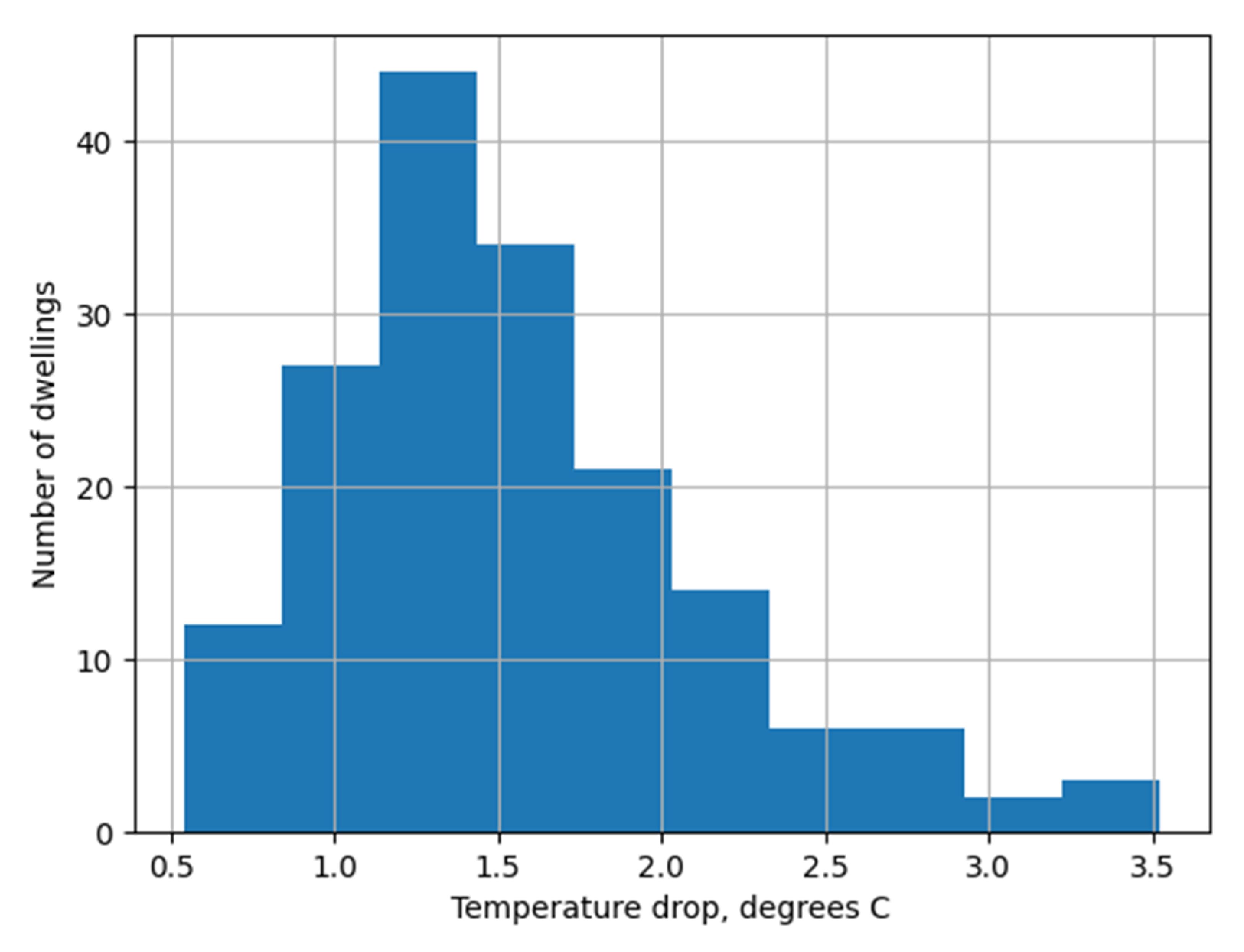
The temperature drops (using a 3-h cooling period and an internal-external temperature difference of 15 °C) for all valid dwellings in the IDEAL dataset are shown in
Figure 4 and summarised in
Table 2.
The temperature drop is calculated from empirical data, using the real cooling observed in occupied homes. A range of factors may therefore affect the calculated temperature drop, as discussed in
Section 5, and the result represents the observed cooling characteristics for the property set in the context of the occupants and of neighbouring dwellings. However, the relationship of the results to building characteristics provides the opportunity to explore the internal validity of the measure and explore whether the trends follow those expected from physical properties.
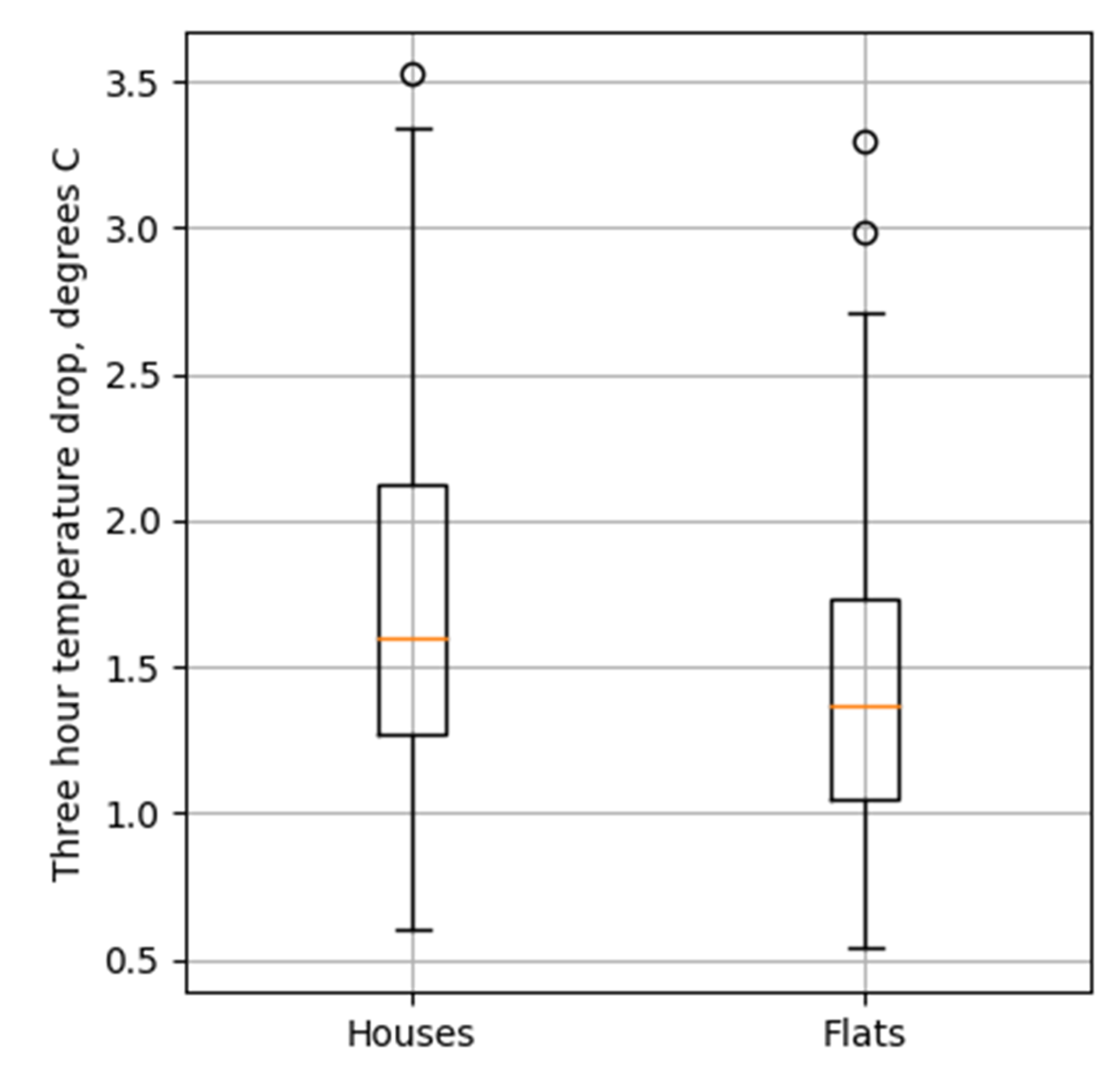
Physical characteristics of buildings which would be expected to result in a lower temperature drop are energy efficiency (e.g., presence of insulation, modern glazing), low number of external walls/floors/ceilings, and thermal mass (heavyweight construction, no internal wall insulation). However, the only building metadata available in the IDEAL dataset is dwelling type, building age and storey level. Of these, the building type is expected to influence the temperature drop, whereby flats, sharing party walls with lower exposed external area, cool more slowly than houses.
Figure 5 shows that the temperature drop for flats over 3 h is indeed less than that for houses in the IDEAL dataset. The mean temperature drop of houses was 1.7, whereas that for flats was 1.43, with a difference between means of 0.27 and
p = 0.0002.
4.3. Contextualising the Results
The spread of observed temperature drops in
Figure 4 indicates that different homes within the test dataset perform differently in terms of their space heating flexibility characteristics. However, for a given home, the temperature drop metric requires contextualisation in terms of whether the value obtained indicates good or poor flexibility potential. Ascribing ‘good’ or ‘poor’ performance to a given home from its temperature drop could be carried out either by comparing it to the current average performance of the building stock (an approach used by [
36] for energy efficiency rating) or according to an external definition of what is ‘good’ and ‘bad’ derived from physics and/or modelling (used by [
37], also for energy efficiency rating). The former approach would require the average temperature drop of the UK stock to be calculated. A large and representative sample is required to create such a rating system, which is not possible using the IDEAL dataset used in this study: it is based in and around the Edinburgh region and is likely to over-represent older, uninsulated buildings made of stone [
38]. The co-location of the IDEAL dataset in one region may also lead to the range of temperature drops in
Figure 4 being narrower than that in the UK stock in general.
By contrast to a rating system based on average performance, a method based on a definition of what constitutes “good” and “bad” performance requires the external construction of such bands. We suggest that such a method should be formed according to the consequences of the temperature drop for the occupants and the needs of the electricity system. Such a method may utilise the temperature drop over a fixed time of relevance to system operation, as here, or the time taken for temperature to drop by a certain amount. Working definitions of an acceptable temperature drop for occupants under demand response are used in the modelling literature to evaluate flexibility potential (see e.g., [
26]. These utilise a set temperature change from an initial operative temperature, for example a 1 °C or 2 °C drop from a setpoint. These definitions are in turn derived from ASHRAE comfort classes [
39]. However, they have not been empirically validated under demand response conditions in homes and more research is needed on thermal comfort during demand response in real homes to characterise temperature changes which are acceptable to occupants.
5. Discussion
The transition from heating via boilers to heat pumps is central to many countries’ strategy to decarbonise heating [
40]. However, the increase in peak loads associated with unmanaged heat pump and electric vehicle charging has been identified as a key challenge that must be addressed to support this transition in a cost-effective manner, with demand side management commonly proposed to mitigate peak loads [
41]. The replacement of a boiler with a heat pump provides a challenge to homeowners in understanding their costs under time-of-use tariffs, and to aggregators and DSOs in managing system services and local network load: what flexibility may be afforded with the heat pump installed, with no previous usage data? This paper introduces a new method to quantify the flexibility of individual dwellings without heat pumps yet installed: their ability to avoid heating use during critical peak periods. The temperature drop metric is introduced as a simple empirical measure of flexibility, informing debate into the further value that may be derived from in-use measured data already associated with the derivation of an in-use heat transfer coefficient, potentially as part of an empirically derived EPC. The discussion of the temperature drop metric here will refer to the performance of empirical EPCs as a reference point, as the closest equivalent empirical metric.
The introduction of the temperature drop metric in this article is intended to begin and contribute to a discussion about the use of building performance data for flexibility metrics, rather than to present a finalised proposal for such a metric and how data would be used. In this section we discuss the benefits and limitations of an empirical flexibility metric, centred around the temperature drop metric, and highlight key further work required to enable measures of this kind to deliver value to a range of stakeholders.
5.1. The Applications of an Empirical Flexibility Metric
The characterisation of individual dwellings on their actual, real-world ability to retain heat has value to a wide range of actors in the energy system. It is beyond the scope of this paper to analyse this in detail, but the following generalisations can be made.
In the short-term (i.e., 1–3 years) the metric itself should allow the householder (directly or through their agent or supplier) to estimate the cost-benefit of running a heat pump flexibly once time-of-use tariffs become more widespread. This could make a significant difference to the economics of the investment decision especially with operational costs rising significantly during the current energy supply crisis and as the government considers how electricity prices can be brought down relative to gas [
42].
In the same way, empirical metrics should also allow policymakers and regulators to segment the housing market more effectively. This can help target limited public funding to where it is likely to be most cost-effective, or in cruder terms, whether a house is “heat pump ready” or not. Conversely, it may also be used to identify properties (centrally or by an installer) that would most benefit from storage to support heat pump operation, such as a thermal store, informing the system specification and potentially highlighting where policy tools may be employed to incentivise storage systems.
In the longer term, as heat pump installations begin to accelerate and the density of heat pumps connected to the grid increases, coincidently with an increase in electric vehicles that require charging, policymakers, researchers and DNOs will need to understand the consequent changes to energy use at different scales. An empirical flexibility metric system will support this analysis, helping to explain trends whilst enabling discussion of the potential impact of measures to increase the flexible operation of heat pumps. This should support better heating system specification, which may be incentivised or regulated, and allow information programmes to be fine-tuned to ensure that the heat pump is operated effectively and allow support and subsidies to be tapered or removed without penalising the householder or exacerbating those in fuel poverty.
A range of businesses could benefit from an empirical flexibility metric system. On the demand-side, heat pump installers and related trades could use the metric to provide a ready-made route to market, subject to appropriate consumer protection measures. On the supply-side, as noted above, flexibility metrics may be used to better understand and manage local network loads as well as support the best use of other energy system assets, such as peaking generation and storage. Deploying empirical flexibility metrics before heat pumps are installed enables grid operators to better manage local networks and plan their upgrade, such as identifying and replacing substation assets.
Furthermore, flexibility metrics have the potential to enable new and innovative business models, for example using the nascent “heat as a service” approach being tested by demand-side energy utilities and equipment manufacturers. On the supply side, there is considerable potential for energy system aggregators to exploit flexibility metrics to develop new services and, potentially reduce operational costs for householders.
Finally, the metric could be combined with other elements of flexibility to yield an overall flexibility rating for the home. This could consider other technical sources of energy shifting beyond building thermal mass, such as dedicated heat storage, hot water storage and batteries. Wider still, further metrics could incorporate social aspects related to availability of these assets [
43].
5.2. Robustness of the Metric
The empirical characterisation of the thermal performance of buildings is conditional on the properties being operated in ways that enable analysis to be undertaken. For example, in the UK’s Smart Meter Enabled Thermal Efficiency Ratings project, none of the eight participating organisations were able to return in-use derived heat transfer coefficient estimates within their confidence intervals of co-heating test results for all 30 properties in the trial, with the best achieving 97% [
23]. Because of the requirement of the observation of a period of falling temperature, the temperature drop metric cannot return a result for all properties.
In this work, the temperature drop metric produced a result for 96% of homes in the test dataset (193 homes), with the main reasons for its failure to give a result in the remaining 4% being the way the heating was used in those properties: either too continuously or too little to allow characterisation of cooling down when heating is switched off. To achieve a rating for all homes, deemed ratings would be required, for example by inference from dwellings in the same location and with similar building characteristics, in line with the virtual EPC calculation methodology used for dwellings without an EPC, set out by [
44].
The average uncertainty on the temperature drop metric as applied to the test dataset was 9%. The required maximum uncertainty on this metric is not clear, depending on the application for which it would be used. Statistical error and accuracy of empirical metrics are important indicators of the metrics’ performance and are currently debated in the context of empirical HTCs. In a recent UK project, different methods and quantities of dwelling metadata were used by participants in a technology competition to give estimates of HTC with statistical uncertainty (calculated using 95% confidence interval) of 6% to 49% [
23]. Furthermore, the central estimates and confidence intervals were compared to a ‘ground truth’ of the HTC, established from a coheating test. In the case of a flexibility metric, further research is required to identify an appropriate ground truth, which may incorporate information on how homes perform when heat pumps are actually installed (see
Section 5.3).
There are several possible sources of systematic error in the temperature drop metric; the first is introduced through the temperature measurements. The temperature drop metric requires data on fuel input, external temperature and internal temperature. External temperature is likely to be obtained from a local weather station, introducing a systematic error for an individual property. Ideally, internal temperature would be the dwelling mean internal temperature; however, in practice a limited number of sensors will be deployed, introducing additional uncertainty. Taking the example of using just one internal temperature measurement, either at a smart thermostat or at a sensor installed to create a thermal efficiency metric, significant differences in temperature drop may be recorded according to the placement of this sensor. Rooms are likely to cool down at different rates depending on their heat loss to other rooms/the outside and their heat gains: Ref. [
45] found a variation in three hour temperature drop of around 0.3 °C if only heated rooms were considered, and 0.9 °C if temperature data from unheated rooms were used as well. This mirrors discussion in empirical HTC literature about the error introduced into the metric when representing whole-house internal temperature with one sensor; Ref. [
46] found a worst case error on HTC of 30%.
The temperature drop metric will vary with a number of occupant specific factors, such as internal heat gains and the thermal mass of the internal contents of the home. For this reason, the metric applies to the ‘home’ (the physical dwelling with the specific occupants living in it) as opposed to simply the building. A new set of occupants in the same dwelling would be expected to change the value of the metric. Since the metric is intended to indicate flexibility potential, it is not necessarily a limitation that the metric is sensitive to occupant factors, since flexibility inevitably depends on occupancy. However, it is important to ensure that the way the dwelling is used during the period of data collection used to create the temperature drop metric is representative of its normal use, in order not to introduce systematic error. This is an important consideration for all empirical metrics which vary with occupant factors (for example, window opening affects the empirical HTC).
5.3. Relevance of the Metric to a Highly Electrified Future of Heating
The temperature drop metric is empirical: it simply characterises the observed behaviour of a property. This has several advantages over a modelled flexibility metric as it encapsulates the real heat loss and effective thermal mass of a property; the latter is difficult to estimate theoretically and time-consuming to derive from calibrated simulation models [
14]. It is also accompanied by an estimate of uncertainty, allowing useful quantification of the range of flexibility potential likely in practice.
However, the temperature drop metric is derived in a different situation (boiler heating) to the situation which it is intended to represent (heat pump heating). It reports on the behaviour of the effective thermal mass activated by the boiler heating, which includes a part of the structural thermal mass, the contents of the dwelling and the thermal mass of the heating system, all of which are at different temperatures. If a heat pump is installed, some of these contributions to stored heat may change:
The heat stored within the effective thermal mass may increase if the heat pump is run more continuously than the previous heating system, as the structural thermal mass (walls, floors etc.) may be kept warmer than previously.
The heat stored within the heating system may change. Increases could arise due to larger radiator thermal masses if new radiators are installed and due to new buffer tanks if these are used. Decreases could arise due to lower operating temperatures. The net effect of these changes will differ by dwelling.
6. Conclusions
Decarbonisation of our energy systems is expected to require a shift from flexible fossil fuel generation towards less flexible generation such as wind power, photovoltaics and nuclear, combined with an increase of electricity use for heat and transport. Heat pumps are projected to provide heat to many properties, with rapid deployment of this technology to replace the incumbent boilers [
47]. Demand side response is, in turn, expected to be required for the cost-effective management of the grid, balancing supply and demand on short timescales. DSR through the interruption of heating provision has been widely proposed and studied using simulation modelling, with the true potential for such participation poorly characterised. This paper has presented the concept of an empirical thermal flexibility metric for homes to indicate their potential to participate in DSR.
A simple metric has been developed to support decarbonisation through informing the specification, billing and system services that may be suitable for retrofitting a home with a heat pump; this aims to initiate and contribute to discussion around the flexibility that may be afforded by a home when switching to a heat pump. The method leverages measurements of temperature and gas to estimate the thermal performance of properties and to provide insight into the rate at which properties cool, and therefore the potential impact of DSR on internal temperatures over a fixed period of reduced consumption.
The temperature drop over a fixed three hour overnight cooling period after the heating has turned off was identified as a simple and easily understood metric. 96% of dwellings in the test dataset of 193 homes returned a viable result, with 4% of dwellings unable to yield a temperature drop due to the type of heating operation in those homes. The mean statistical error was 9%, similar to that of equivalent empirical metrics such as for estimation the heat transfer coefficient. The presented method requires refinement and further research, to better understand the potential impact of gains, occupant factors and heat transfer for neighbouring properties, and the development of alternative methods may prove valuable. Any methods to characterise the flexibility of homes that are heated intermittently with boilers when they are retrofitted with continuously operated heat pumps require testing for external validity to ascertain whether the rating ascribed corresponds to how the dwelling loses heat after a heat pump is installed, as well as further testing on a representative large sample of homes.
The empirical flexibility metric uses the same data as current methods of producing an empirically based estimate for the heat transfer coefficient, potentially as part of future EPCs and adding very little cost. Furthermore, empirical flexibility ratings for domestic buildings would provide value to a range of actors. Householders can be provided with an estimate of financial savings from time of use tariffs, guided to appropriate tariffs and supported with decision making in the specification of their system, supporting heat pump uptake. Distribution network operators can estimate local loads to better manage the network through understanding how many heat pumps may need to run during critical peak times. Reliable information on dwelling thermal response can be used to develop business models for heat-as-a-service providers and aggregators and for government to strategically plan for flexibility response for timescales up to a few hours. For example, the (non-representative) set of 193 test dwellings showed on average 1.5 °C temperature drop over a 3-h period, which may exceed occupants’ tolerances if no heating at all were used in this time—further work is needed in parallel to ascertain acceptable temperature change limits and how to operate heat pumps in order to not exceed them. We also highlight that pre-heating of properties was not undertaken in this study; the potential to thermally charge homes prior to a DSR period and consequent impact on thermal comfort and energy reduction during the DSR event is an important and related focus for further research.
Many countries currently have, or are developing, policies to incentivise the decarbonisation of heating through the installation of heat pumps, aiming to rapidly increase their market penetration. Methods that calculate and communicate energy use data and cooling performance of properties can support householders, industry and government in decision making, providing insights into the DSR potential, appropriate tariffs, system specification and network loads. Empirical flexibility metrics could, following further development and testing, form part of this information, supporting the transition to a decarbonised energy system.
Author Contributions
Conceptualization, J.C. and C.E.; Data curation, J.C.; Formal analysis, J.C. and D.M.; Funding acquisition, C.E.; Investigation, J.C., P.M. and C.E.; Methodology, J.C. and D.M.; Software, J.C.; Validation, J.C.; Visualization, J.C.; Writing—original draft, J.C.; Writing—review and editing, J.C., D.M., P.M. and C.E. All authors have read and agreed to the published version of the manuscript.
Funding
This work was funded through the Centre for Research in Energy Demand Solutions (EP/R035288/1).
Institutional Review Board Statement
Not applicable.
Informed Consent Statement
Not applicable.
Data Availability Statement
Not applicable.
Conflicts of Interest
The authors declare no conflict of interest.
Appendix A
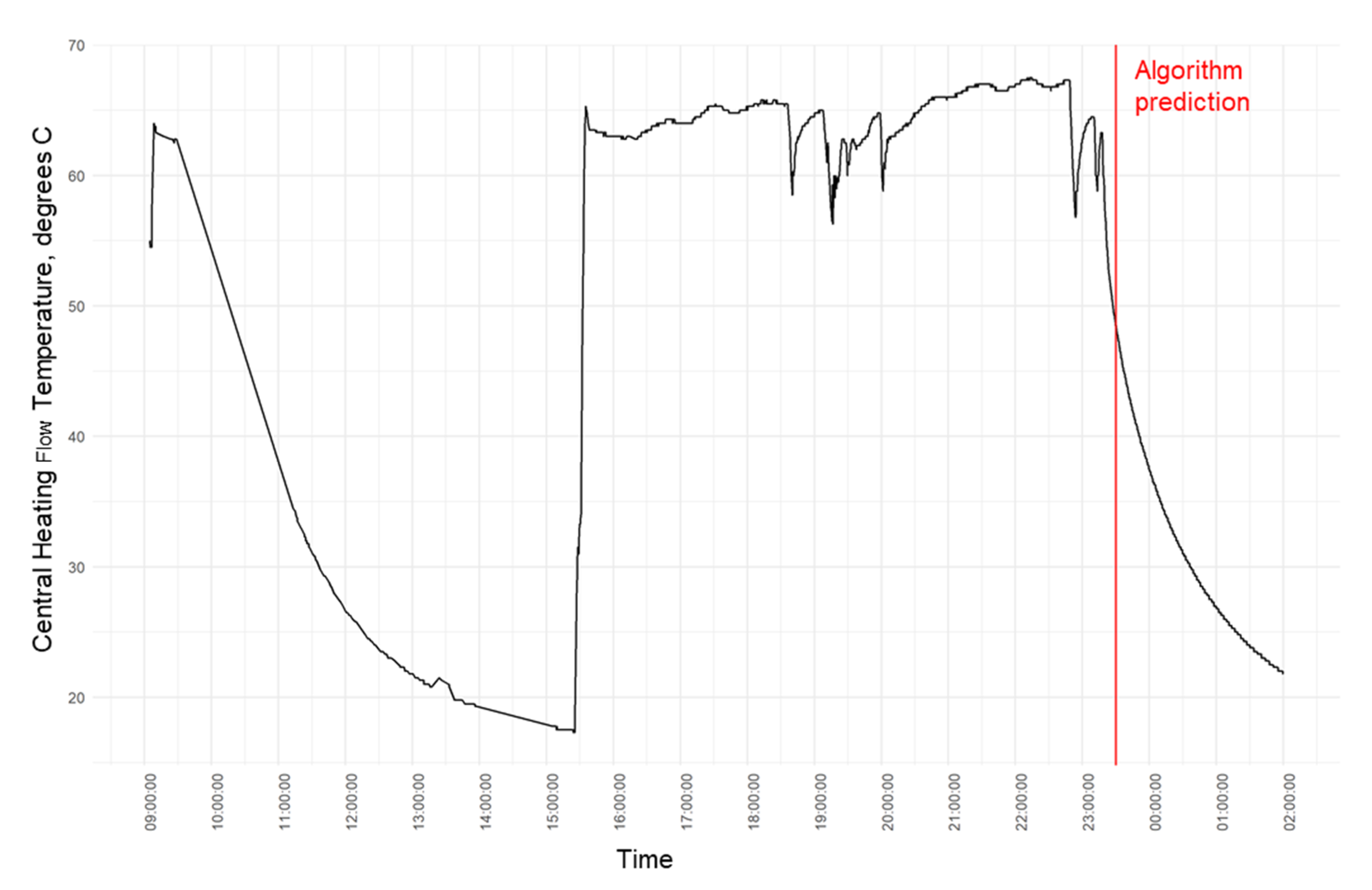
The next two graphs are examples of the heating operation algorithm’s prediction superimposed on ground truth data (12-s central heating flow temperature).
Figure A1.
Comparison of the algorithm’s output to the ground truth for IDEAL home no. 135. Heating operation algorithm correctly predicts time of final heating switch off, to the nearest half hour.
Figure A1.
Comparison of the algorithm’s output to the ground truth for IDEAL home no. 135. Heating operation algorithm correctly predicts time of final heating switch off, to the nearest half hour.
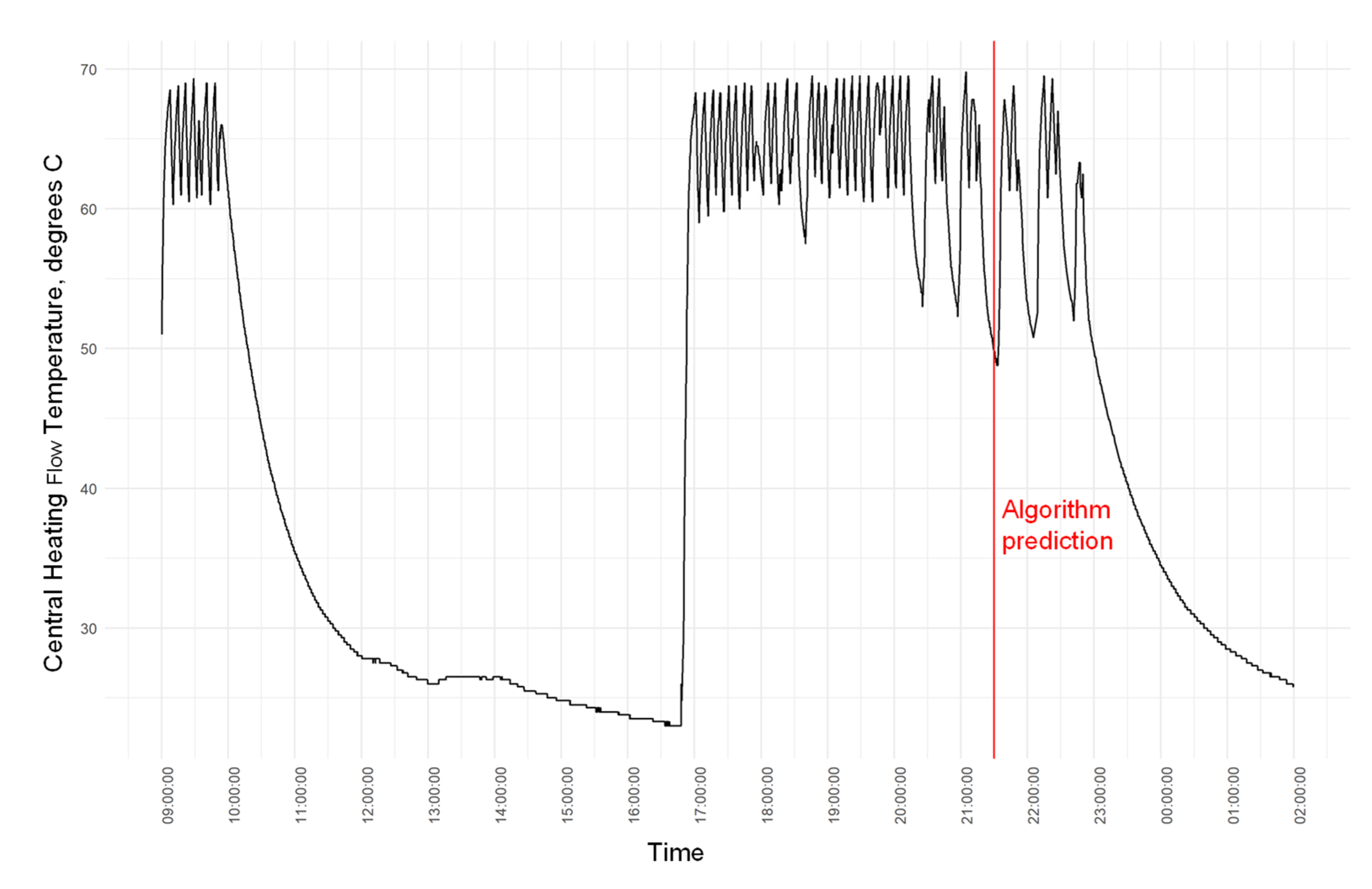
Figure A2.
Comparison of the algorithm’s output to the ground truth for IDEAL home no. 137. Heating operation algorithm incorrectly predicts time of final heating switch off.
Figure A2.
Comparison of the algorithm’s output to the ground truth for IDEAL home no. 137. Heating operation algorithm incorrectly predicts time of final heating switch off.
References
- International Energy Agency. Net Zero by 2050: A Roadmap for the Global Energy Sector; International Energy Agency: Paris, France, 2021. [Google Scholar]
- International Energy Agency (Ed.) Net Zero by 2050–Data Product; International Energy Agency: Paris, France, 2021. [Google Scholar]
- Eyre, N. From using heat to using work: Reconceptualising the zero carbon energy transition. Energy Effic. 2021, 14, 77. [Google Scholar] [CrossRef]
- Steegh, R.; van Cuijk, T.; Pourasghar-khomami, D. Grid management system to solve local congestion. In Proceedings of the 25th International Conference on Electricity Distribution, Madrid, Spain, 3–6 June 2019. [Google Scholar]
- Watson, S.D. Predicting the Additional GB Electricity Demand Resulting from a Widespread Uptake of Domestic Heat Pumps; Loughborough University: Loughborough, UK, 2020. [Google Scholar]
- Li, P.-H.; Pye, S. Assessing the benefits of demand-side flexibility in residential and transport sectors from an integrated energy systems perspective. Appl. Energy 2018, 228, 965–979. [Google Scholar] [CrossRef]
- Reynders, G.; Lopes, R.A.; Marszal-Pomianowska, A.; Aelenei, D.; Martins, J.; Saelens, D. Energy flexible buildings: An evaluation of definitions and quantification methodologies applied to thermal storage. Energy Build. 2018, 166, 372–390. [Google Scholar] [CrossRef]
- BRE Trust. The Housing Stock of the United Kingdom; Building Research Establishment: Watford, UK, 2017. [Google Scholar]
- BRE Trust. The Government’s Standard Assessment Procedure for Energy Rating of Dwellings, Version 10.2.; BRE: Watford, UK, 2022. [Google Scholar]
- Crawley, J.; McKenna, E.; Gori, V.; Oreszczyn, T. Creating domestic building thermal performance ratings using smart meter data. Build. Cities 2020, 1, 1–13. [Google Scholar] [CrossRef]
- Arteconi, A.; Mugnini, A.; Polonara, F. Energy flexible buildings: A methodology for rating the flexibility performance of buildings with electric heating and cooling systems. Appl. Energy 2019, 251, 113387. [Google Scholar] [CrossRef]
- Kelly, N.; Cowie, A.; Flett, G. Assessing the ability of electrified domestic heating in the UK to provide unplanned, short-term responsive demand. Energy Build. 2021, 252, 111430. [Google Scholar] [CrossRef]
- Sperber, E.; Frey, U.; Bertsch, V. Reduced-order models for assessing demand response with heat pumps–Insights from the German energy system. Energy Build. 2020, 223, 110144. [Google Scholar] [CrossRef]
- Allison, J.; Cowie, A.; Galloway, S.; Hand, J.; Kelly, N.J.; Stephen, B. Simulation, implementation and monitoring of heat pump load shifting using a predictive controller. Energy Convers. Manag. 2017, 150, 890–903. [Google Scholar] [CrossRef] [Green Version]
- IEA-EBC. EBC Annex 71: Building Energy Performance Assessment Based on In-situ Measurements. 23/05/2019. Available online: http://annex71.iea-ebc.org/projects/project?AnnexID=71 (accessed on 21 June 2022).
- UK Government. Smart Meter Enabled Thermal Efficiency Ratings (SMETER) Innovation Programme. 2019. Available online: https://www.gov.uk/guidance/smart-meter-enabled-thermal-efficiency-ratings-smeter-innovation-programme (accessed on 21 June 2022).
- Jenkins, D.; Simpson, S.; Peacock, A. Investigating the consistency and quality of EPC ratings and assessments. Energy 2017, 138, 480–489. [Google Scholar] [CrossRef]
- Crawley, J.; Biddulph, P.; Northrop, P.J.; Wingfield, J.; Oreszczyn, T.; Elwell, C. Quantifying the Measurement Error on England and Wales EPC Ratings. Energies 2019, 12, 3523. [Google Scholar] [CrossRef] [Green Version]
- Christensen, T.H.; Gram-Hanssen, K.; de Best-Waldhober, M.; Adjei, A. Energy retrofits of Danish homes: Is the Energy Performance Certificate useful? Build. Res. Inf. 2014, 42, 489–500. [Google Scholar] [CrossRef]
- Fosas, D.; Nikolaidou, E.; Roberts, M.; Allen, S.; Walker, I.; Coley, D. Towards active buildings: Rating grid-servicing buildings. Build. Serv. Eng. Res. Technol. 2020, 42, 129–155. [Google Scholar] [CrossRef]
- Gleue, M.; Unterberg, J.; Löschel, A.; Grünewald, P. Does demand-side flexibility reduce emissions? Exploring the social acceptability of demand management in Germany and Great Britain. Energy Res. Soc. Sci. 2021, 82, 102290. [Google Scholar] [CrossRef]
- Love, J.; Smith, A.Z.; Watson, S.; Oikonomou, E.; Summerfield, A.; Gleeson, C.; Lowe, R. The addition of heat pump electricity load profiles to GB electricity demand: Evidence from a heat pump field trial. Appl. Energy 2017, 204, 332–342. [Google Scholar] [CrossRef]
- BEIS. Technical Evaluation of SMETER Technologies (TEST) Project; 2022. Available online: https://assets.publishing.service.gov.uk/government/uploads/system/uploads/attachment_data/file/1050881/smeter-innovation-competition-report.pdf (accessed on 21 June 2022).
- Hoffman, M.E.; Feldman, M. Calculation of the thermal response of buildings by the total thermal time constant method. Build. Environ. 1981, 16, 71–85. [Google Scholar] [CrossRef]
- Johra, H.; Heiselberg, P.; Dréau, J.L. Influence of envelope, structural thermal mass and indoor content on the building heating energy flexibility. Energy Build. 2019, 183, 325–339. [Google Scholar] [CrossRef]
- Reynders, G.; Nuytten, T.; Saelens, D. Potential of structural thermal mass for demand-side management in dwellings. Build. Environ. 2013, 64, 187–199. [Google Scholar] [CrossRef]
- Wang, S.; Kang, Y.; Yang, Z.; Yu, J.; Zhong, K. Numerical study on dynamic thermal characteristics and optimum configuration of internal walls for intermittently heated rooms with different heating durations. Appl. Therm. Eng. 2019, 155, 437–448. [Google Scholar] [CrossRef]
- Jones, P. Thermal Design of Buildings: Understanding Heating, Cooling and Decarbonisation; Crowood Press: Marlborough, UK, 2021; Available online: https://orca.cardiff.ac.uk/id/eprint/144075/ (accessed on 21 June 2022).
- Karlsson, F.; Fahlén, P. Impact of design and thermal inertia on the energy saving potential of capacity controlled heat pump heating systems. Int. J. Refrig. 2008, 31, 1094–1103. [Google Scholar] [CrossRef]
- Buswell, R.; Webb, L.; Cosar-Jorda, P.; Marini, D.; Brownlee, S.; Thomson, M.; Kalawsky, R. LEEDR Project Home Energy Dataset; Lougboury University: Loughborough, UK, 2018. [Google Scholar]
- Tabatabaei, S.A.; van der Ham, W.; Klein, M.; Treur, J. A Data Analysis Technique to Estimate the Thermal Characteristics of a House. Energies 2017, 10, 1358. [Google Scholar] [CrossRef] [Green Version]
- Hollick, F.P.; Gori, V.; Elwell, C.A. Thermal performance of occupied homes: A dynamic grey-box method accounting for solar gains. Energy Build. 2020, 208, 109669. [Google Scholar] [CrossRef]
- Pullinger, M.; Kilgour, J.; Goddard, N. The IDEAL household energy dataset, electricity, gas, contextual sensor data and survey data for 255 UK homes. Sci. Data 2021, 8, 146. [Google Scholar] [CrossRef]
- Alzaatreh, A.; Mahdjoubi, L.; Gething, B.; Sierra, F. Disaggregating high-resolution gas metering data using pattern recognition. Energy Build. 2018, 176, 17–32. [Google Scholar] [CrossRef] [Green Version]
- Bacher, P.; de Saint-Aubain, P.A.; Christiansen, L.E.; Madsen, H. Non-parametric method for separating domestic hot water heating spikes and space heating. Energy Build. 2016, 130, 107–112. [Google Scholar] [CrossRef] [Green Version]
- Lomas, K.; Beizaee, A.; Allinson, D.; Haines, V.; Beckhelling, J.; Loveday, D.; Porritt, S.; Mallaband, B.; Morton, A. A domestic operational rating for UK homes: Concept, formulation and application. Energy Build. 2019, 201, 90–117. [Google Scholar] [CrossRef]
- SMHI. SMHI ENERGI-INDEX.; Swedish Meteorological and Hydrological Institute: Norrkoping, Sweden, 2018. [Google Scholar]
- Pullinger, M.; Berliner, N.; Goddard, N.; Shipworth, D. Domestic heating behaviour and room temperatures: Empirical evidence from Scottish homes. Energy Build. 2022, 254, 111509. [Google Scholar] [CrossRef]
- ISO 7730: 2005; Ergonomics of the Thermal Environment-Analytical Determination and Interpretation of Thermal Comfort using Calculation of the PMV and PPD Indices and Local Thermal Comfort Criteria. ISO: Geneva, Switzerland, 2005.
- Vivid Economics & Imperial College. International Comparisons of Heating, Cooling and Heat Decarbonisation Policies; Department of Business, Energy and Industrial Strategy: London, UK, 2017. [Google Scholar]
- Kanakadhurga, D.; Prabaharan, N. Demand side management in microgrid: A critical review of key issues and recent trends. Renew. Sustain. Energy Rev. 2022, 156, 111915. [Google Scholar] [CrossRef]
- HM Government. Heat and Buildings Strategy; Crown Copyright: London, UK, 2021. [Google Scholar]
- Powells, G.; Fell, M.J. Flexibility capital and flexibility justice in smart energy systems. Energy Res. Soc. Sci. 2019, 54, 56–59. [Google Scholar] [CrossRef] [Green Version]
- Steadman, P.; Evans, S.; Liddiard, R.; Shimizu, D.; Ruyssevelt, P.; Humphrey, D. Building stock energy modelling in the UK: The 3DStock method and the London Building Stock Model. Build. Cities 2020, 1, 100–119. [Google Scholar] [CrossRef]
- Martin-Vilaseca, A.; Crawley, J.; Shipworth, M.; Elwell, C. Living with demand response: Insights from a field study of DSR using heat pumps. In Proceedings of the ECEEE, Hyeres, France, 6–11 June 2022. [Google Scholar]
- Senave, M.; Roels, S.; Verbeke, S.; Saelens, D. Analysis of the influence of the definition of the interior dwelling temperature on the characterization of the heat loss coefficient via on-board monitoring. Energy Build. 2020, 215, 109860. [Google Scholar] [CrossRef]
- United Nations Environment Programme. 2021 Global Status Report for Buildings and Construction: Towards a Zero-Emission, Efficient and Resilient Buildings and Construction Sector; United Nations Environment Programme: Nairobi, Kenya, 2021. [Google Scholar]
| Publisher’s Note: MDPI stays neutral with regard to jurisdictional claims in published maps and institutional affiliations. |
© 2022 by the authors. Licensee MDPI, Basel, Switzerland. This article is an open access article distributed under the terms and conditions of the Creative Commons Attribution (CC BY) license (https://creativecommons.org/licenses/by/4.0/).


