Static Analysis and Optimization of Voltage and Reactive Power Regulation Systems in the HV/MV Substation with Electronic Transformer Tap-Changers

Abstract

The quality of electricity is a very important indicator. The durability and reliable operation of all connected devices depend on the quality of the network voltage. Rapid changes in loads, changes in network connections and the presence of uncontrolled energy sources require the development of new voltage regulation systems. This requires voltage regulation systems capable of responding quickly to sudden voltage changes. In substations with control transformers, it is possible thanks to the use of semiconductor tap changers. Moreover, voltage regulation and reactive power compensation systems should be built as one system. This is due to the close dependence of voltage and reactive power in the network node. Therefore, it was proposed to use artificial intelligence methods to build a new voltage regulation and reactive power compensation system using all measurement voltages of network nodes. In the first stage of the research, active and reactive powers, as well as the voltage of the reference node, were selected for 6420 periods of the mains voltage. The simulation results were compared for the classic voltage regulation system with semiconductor tap changers and the evolution algorithm based on voltage measurements from the entire MV network. A significant improvement in the quality of voltage regulation with the use of an evolutionary algorithm was demonstrated. Then, a second set of input data with increased values of reactive power was generated. The results of the evolutionary algorithm after the application of the classic, independent reactive power compensation system and two-criteria optimization were compared. It has been shown that only the two-criteria optimization algorithm keeps both |tgφ| within the acceptable range and the quality of voltage regulation is the best. The article compares different working algorithms for semiconductor tap changers.

1. Introduction

The currently operated voltage regulation systems in HV/MV stations use only the transformer voltage on the MV side. The analysis of voltage regulation systems using electromechanical tap-changers of the transformer is presented in [1,2]. The design of a traditional tap-changer is shown in Figure 1a. The view of the power transformer with the on-load tap-changer is shown in Figure 1b.

Measurements of electrical quantities in MV networks (smart grids) are more often available. There are works on the use of semiconductor tap changers for voltage regulation in HV, MV and LV networks [3,4,5,6,7,8,9,10,11,12]. The differences between the electromechanical and semiconductor control algorithms are presented, among others, in [13,14]. There are applications of power semiconductors in high-voltage and high-power circuits, e.g., [15]. There is a need to develop optimally integrated voltage regulation and reactive power compensation [16,17,18,19,20]. It is indispensable to use artificial intelligence methods to design voltage regulation and reactive power compensation systems [21,22].

Due to the increase in the number of operating non-linear loads in the power grid, problems with the quality of electricity appear. For this reason, a new power electronic device was proposed to be installed in the substation [23,24]. The paper presents a novel strategy of predictive control for shunt active power filter (APF). The proposed control includes feedback from the supply current and combines the advantages of control in an open and closed loop—the transient response speed after changing the load current and a very high compensation efficiency. The high quality of the compensation current also results from the use of predictive algorithms in the control, as well as from the fact of connecting the converter to the network via the LCL circuit. The article presents the results of simulation tests of the proposed control algorithm. In [24] is presented an active filter connected in parallel to the power supply and electric energy receivers. It is made up of two sections of the coil sections L1 and L2, with a capacitor section connected in parallel between them. The other end of the filter is connected to six power transistors and a capacitor. The article demonstrates the effective filtration of harmonics up to the 50th. This type of device can be used in power stations to which industrial plants generating disturbances are connected, e.g., steel mills. These are examples of the use of automation and power electronics in power networks. Another example of the use of power electronics in the power industry is presented in [25].

1.1. Solid-State on-Load Tap Changer Technology

On-load tap changers have been used for a long time in HV substations. Currently, electromechanical tap changers are used. They have considerable disadvantages, including the formation of an electric arc on the contacts, limited switching frequency and limited total switching frequency, e.g., up to several times a day. Currently, there are more and more receivers and generators in the power grid with high dynamics of power changes. As a result, there is a need to build a voltage regulation system with high switching dynamics. The use of semiconductor tap changers enables quick voltage regulation. AC connectors should be used here. IGBT power transistors are currently the most popular in power electronics.

Currently, SiC-based power semiconductors made in the form of IGBT transistors have the highest switching frequencies. At the same time, the permissible operating temperature of SiC semiconductor elements is higher than the others. Thus, such elements can be used in the power industry. The regulating winding in HV/MV transformers is on the higher voltage side. The windings of these transformers on the 110 kV side, i.e., HV, are star-connected. One end of the regulating winding is connected to the neutral conductor, the other end to the working winding. The phase voltage of the entire winding is 63.5 kV. Assuming that the control system regulation range should be from −20% to +20%, the required reverse voltage for semiconductor modules is 12.7 kV.

For publicly available high-voltage single semiconductor elements, it is at most 6.5 kV, e.g., 5SNA0400J650100 from ABB (collector current Ic = 400 A, turn-on delay time maximum is 700 ns, turn-off delay time maximum is 1700 ns); however, this semiconductor module is very expensive. It is possible to build modules for higher voltages, ensuring that the elements in series change the switching state practically simultaneously. In addition, during the construction of the module, a reserve of voltage resistance is additionally provided.

In [4] is presented a prototype of a tap changer controlled by a microcontroller. The prototype has five tap changers realized by means of pairs of thyristors. This applies to the low voltage 230/115 VAC system. For the correct commutation, the detection of current through zero was used (in regulating winding). This was realized by Zero Current Detection Card. The system was tested with a slight change in load or a slight change in input voltage but is working properly. The article does not present the implemented algorithm in the microcontroller or the use of voltage measurement on the primary side of the transformer

Any variation in the output voltage of the distribution transformer will be sensed by the microcontroller and compared with the reference value as per the program. This will produce the appropriate command to trigger the appropriate pair of anti-parallel thyristors for change in the suitable tapping of the transformer. The system stability is improved because of the quick response. Because of static devices, the maintenance cost is reduced due to the elimination of frequent sparking. The output voltage can be regulated in the range of ±5 V of nominal voltage [4].

In article [11] is presented the construction of a transformer semiconductor tap-changer regulator. Figure 2 shows the structure of the proposed voltage regulator controlling the semiconductor tap changers. The first block introduces a deadband that prevents oscillations when a voltage error changed the value on the border of two adjacent taps. The electronic tap changer operates fast and real-time measurement of the RMS value of the regulation bus is expected. One of the best substitutions for the RMS value of the voltage is the instantaneous RMS value of the voltage. Compensating block is used instead of a delay block, which is a special type of compensator. In [26], it has been shown that the use of an integrator in the compensating block of an electronic tap-changer seems interesting from a quality point of view. The integrator produces typically the delay proportional to DB, and it also has memory. The integrator gain influences the stability and also the speed of the system. The tap changer control is not a continuous control. For this reason, a quantization block is required. A discrete value of the tap number will be assigned to the continuous value of the voltage error. Due to the fact that the tap switching should take place when a current close to zero flows through the winding. Then, there are no overvoltages and disturbances. The S&H block remembers the selected tap number and, after receiving the permission to switch from the zero-crossing current detection block, performs the tap change-over. The loop-up table for the selected tap number displays the states of semiconductor switches similar to

Table 1. Switches states depending on the OLTC position.

OLTC Position	Percentage Change in Voltage on the MV Side	Ratio in p.u.	K1	K2	K3	K4	K5	K6	K7	K8	K9	K10	K11	K12	K13	K14
1	−20.00%	0.80	1			1				1	1			1	1
2	−19.00%	0.81	1			1				1	1	1			1
3	−18.00%	0.82	1			1				1		1	1		1
4	−17.00%	0.83	1			1			1		1			1	1
5	−16.00%	0.84	1			1			1		1	1			1
6	−15.00%	0.85	1			1			1			1	1		1
7	−14.00%	0.86	1			1		1			1			1	1
8	−13.00%	0.87	1			1		1			1	1			1
9	−12.00%	0.88	1			1		1				1	1		1
10	−11.00%	0.89	1			1	1				1			1	1
11	−10.00%	0.90	1			1	1				1	1			1
12	−9.00%	0.91	1		1					1	1	1			1
13	−8.00%	0.92	1		1					1		1	1		1
14	−7.00%	0.93	1		1				1		1			1	1
15	−6.00%	0.94	1		1				1		1	1			1
16	−5.00%	0.95	1		1				1			1	1		1
17	−4.00%	0.96	1		1			1			1			1	1
18	−3.00%	0.97	1		1			1			1	1			1
19	−2.00%	0.98	1		1			1				1	1		1
20	−1.00%	0.99	1		1		1				1			1	1
21	0.00%	1.00	1	1
22	1.00%	1.01		1	1		1				1			1		1
23	2.00%	1.02		1	1			1				1	1			1
24	3.00%	1.03		1	1			1			1	1				1
25	4.00%	1.04		1	1			1			1			1		1
26	5.00%	1.05		1	1				1		1	1	1			1
27	6.00%	1.06		1	1				1		1			1		1
28	7.00%	1.07		1	1				1		1			1		1
29	8.00%	1.08		1	1					1		1	1			1
30	9.00%	1.09		1	1					1	1	1				1
31	10.00%	1.10		1		1	1				1	1				1
32	11.00%	1.11		1		1	1				1			1		1
33	12.00%	1.12		1		1		1				1	1			1
34	13.00%	1.13		1		1		1			1	1				1
35	14.00%	1.14		1		1		1			1			1		1
36	15.00%	1.15		1		1			1			1	1			1
37	16.00%	1.16		1		1			1		1	1				1
38	17.00%	1.17		1		1			1		1			1		1
39	18.00%	1.18		1		1				1		1	1			1
40	19.00%	1.19		1		1				1	1	1				1
41	20.00%	1.20		1		1				1	1			1		1

.

1.2. Volt Var Control

In many stations, reactive power compensation is required. Independent voltage regulation and reactive power compensation may cause deterioration of the operation of at least one of them. For example, when the voltage in the substation is close to the upper acceptable limit, i.e., 1.1 Un, and the reactive power compensation system additionally switches on capacitors, it may lead to the exceeding of this limit. This is due to the dependence of the node voltage and reactive power. For this reason, it is necessary to build integrated systems of voltage regulation and reactive power compensation called Volt Var Control or Volt/Var Management System. This is especially important when distributed generation or energy storage occurs in the distribution network.

2. Materials and Methods

2.1. Assumptions and Description

Input data, such as the voltage of the balancing (refencing) node and the active and reactive power of the load nodes, were randomized with certain assumptions. Then, the tested algorithm set the tap number and possibly turned on the appropriate number of batteries for reactive power compensation. In the calculation of the power flow, the voltages in all network nodes were determined. The input data sets were 6420 in size. On this basis, histograms were created, which allows to graphically present the range of changes and the frequency of occurrence of a given value of the voltage error, the coefficient tgφ.

The tested network consists of a referencing node number one in the depths of the network, with the network impedance calculated on the basis of the short-circuit power on the HV busbars of the 110/15 kV substation (equivalent to the rest of the power system—Thevenin’s theorem). The structure of the network is presented in Figure 1 below. Nodes 4 to 15 are receiving nodes for which the value of active and reactive power is randomized, as in the actual network operation (the load powers of individual stations 15/0.4 change over time). The drawing of relative power values in individual load nodes was performed according to the following dependence (1) P,Q in p.u.:

$$\begin{array}{c}\hfill \underset{i=4}{\overset{15}{{\displaystyle \wedge }}}{P}_i=random\left(0.3:1\right)\hfill \\ \hfill \mathrm{where} random-\mathrm{random} \mathrm{number} \mathrm{of} \mathrm{uniform} \mathrm{distribution} \hfill \end{array}$$

(1)

The apparent power of a station in relative units is equal to 1: S_i = 1 p.u. Due to the apparent power of the station, the maximum reactive power is (2):

$$\underset{i=4}{\overset{15}{{\displaystyle \wedge }}}{Q}_{i\_\max }=\sqrt{1-P_i^2}$$

(2)

Moreover, assuming that the maximum reactive power cannot exceed 60% of the value of the randomly selected active power in the node, we finally obtain the maximum reactive power (3):

$$\underset{i=4}{\overset{15}{{\displaystyle \wedge }}}{Q}_{\max \_i}=\min \left(Q_{i\_\max };0.6\ast P_i\right)$$

(3)

The reactive power at the node i is (4):

$$\underset{i=4}{\overset{15}{{\displaystyle \wedge }}}{Q}_i=random\left(0.3:Q_{\max \_i}\right)$$

(4)

Moreover, the voltage at node 1 is also variable in time and randomized (uniform distribution) in the range from 0.7 to 1.3 Un. The structure of the studied network is presented in Figure 3. Availability of online voltage measurements at all MV nodes and nodal powers was assumed. In order to perform the simulation, the Newton–Raphon method was used for 6420 samples (input data). The input data are the power consumed in the load nodes (P, Q) and the voltage of the referencing node no 1. The output data are voltages at 15 kV nodes and power flows.

The control winding was designed to be switched with semiconductor switches in such a way as to ensure smooth voltage regulation with a minimum number of taps and switches—Figure 4. Table 1 presents the switch states configuration depending on the required ratio.

In order to optimize the voltage regulation, the node voltage evaluation function was determined according to the Formula (5):

$$\begin{array}{c}{e}_i=\left|1-U_i\right|\\ f\left(U_i\right)=\{\begin{array}{c}0, where e_i\le 0.05\\ {\left(e_i-0.05+1\right)}^6-1,where e_i>0.05 and e_i\le 0.1\\ {\left(e_i-0.1+1\right)}^9-1+0.340095640625 where e_i>0.1\end{array}\end{array}$$

(5)

where U_i—The voltage module in the relative units of the node i, where i = 3.15.

The diagram of the node voltage evaluation function is shown in Figure 5. This function is continuous so that optimization is convergent. It is an internal function of the penalty for the voltage acceptable limit ±10% Un. The penalty function becomes non-zero after exceeding the absolute value of the error above 5% (see Figure 5). With an increase in the absolute value of the voltage error, the derivative of this function also increases. This provides a choice of optimization solutions with small voltage deviations in the nodes than solutions with large voltage deviation in at least one node.

For the entire network, the evaluate function is the sum of all MV node ratings:

$$J_m={\displaystyle \sum }_{i=4}^{15}f(U_{i,m}\left(z;U_{ref,m};P_{rec,m};Q_{rec,m}\right))$$

(6)

where: i—number node in 15 kV network, m—number sample of input data set, z_m—optimal number state regulation (see Table 1), U_ref,m—voltage of referencing node for m sample—input data, P_rec,m, Q_rec,m—vector active/reactive power for all receiving node in m sample—input data, U_i,m—the voltage at the node i for the input data set m—result of power flow analysis, f(U_i)—evaluation function for voltage node (5).

Optimization formula is (7):

$$\underset{m=1}{\overset{6420}{{\displaystyle \wedge }}}\min ({\displaystyle \sum }_{i=4}^{15}f\left(U_{i,m}\left(z_m;U_{ref,m};P_{rec,m};Q_{rec,m}\right)\right)$$

(7)

The evaluation of the operation of the control system was determined as (8):

$$J={\displaystyle \sum }_{m=1}^{6420}\left({\displaystyle \sum }_{i=4}^{15}f(U_{i,m}\left(z_m;U_{ref,m};P_{rec,m};Q_{rec,m}\right)\right)$$

(8)

This is the sum of the whole network scores for all input data samples.

2.2. Simulation Research Using Power Flow Calculations in Power Network

The simulations were carried out in several variants. In the first one without voltage regulation and reactive power compensation, the relative transformer ratio was equal to 1.

The second variant is the classic regulation with semiconductor tap changers without reactive power compensation. The third variant is the use of evolutionary algorithms to determine the optimal tap using the voltage values in all load nodes. Results were presents in Section 3.1.

The fourth variant is the inclusion of the classic algorithm for connecting capacitor banks for the variant without voltage regulation. The fifth and sixth variant is also the launch of the classic algorithm for reactive power compensation for variants of the classic voltage regulation and optimization of the tap number using evolutionary algorithms.

The calculations were made in Matlab. MatPower was used to calculate voltages and power flow in the power grid.

The evolutionary algorithm is widely used to solve various optimization tasks or control systems in many fields of science, such as in [27,28,29] or other methods of artificial intelligence [30,31]. The eventual algorithm was started with the following Matlab commands ga.

It is an integer optimization with a limitation of the optimization variable value ranging from 1 to 41. The population size was set to 20 individuals. The maximum number of generations is 500.

2.3. Simulation Research Using Power Flow Calculations in Power Network with High Reactive Power Consumption

For high-reactive power data, the formula was applied regardless of the actual active power and the allowable apparent power. The remaining parameters of the simulation were left as in the previous one.

In that variant the reactive power at the node i is (9). Compared to Formula 4, the lower limit has been increased to 0.7 value of active power P_i and the upper limit to 0.8 p.u.:

$$\underset{i=4}{\overset{15}{{\displaystyle \wedge }}}{Q}_i=random\left(0.7·P_i:0.8\right)$$

(9)

During the generation of new data, it was taken into account that not all the results obtained (reactive power in load nodes) will allow for the execution of power and voltage flow calculations. For this reason, after drawing the reactive power in load nodes, the input data was verified by means of power flow calculations. The remaining parameters, such as the referencing node voltages and active powers in nodes 4 to 15, remained the same as in the previous set of input data, i.e., 6420 periods.

Then, for the data thus obtained, an evolutionary algorithm was run in order to implement optimal voltage regulation. Moreover, the required value of reactive power for compensation and the number of capacitor banks with a capacity of 30 kVAr were determined. The next step was to update the power grid model, taking into account capacitor banks. For the obtained results, the calculations of voltages and power flow were made again for the determined degree of regulation control and connected batteries for reactive power compensation. Results were presented in Section 3.2.

2.4. Simulation Research Using Power Flow Calculations in Pareto Multi-Criteria Optimizing

Simultaneous and integrated voltage regulation and reactive power compensation are necessary to ensure correct operation of the substation. The problem of multi-criteria optimization arises. On the one hand, the system should ensure correct voltage values in the entire power network and at the same time compensate the reactive power to the required value—use of multi-criteria optimization—Pareto—simultaneous voltage and reactive power regulation. From the set of non-dominated solutions, a solution was selected that meets the voltage quality requirements with as much as possible reactive power compensation for each set of input data.

The first optimization criterion is minimizing the entire network, the evaluate function is the sum of all MV node ratings (6). The second criterion is the reactive power compensation assessment. According to the legal requirements, the reactive power should not exceed the value determined by the relationship (10):

$$\left|tg\varphi =\frac{Q}{P}\right|\le 0.4$$

(10)

The reactive power compensation evaluation function should have a value of 0 when the reactive power does not exceed the value of 40% of active power. The evaluation function used is as follows (11):

$$\begin{array}{c}tg{\varphi }_{T,m}=\{\begin{array}{c}\frac{Q_{T,m}}{P_{T,m}},where Q_{T,m}\ge 0 and P_{T,m}>0\\ 0,other case\end{array}\\ \begin{array}{c}\begin{array}{c}{Q}_{2compens}=\{\begin{array}{c}0, where tg{\varphi }_{T,m}\le 0.4\\ Q_{T,m}-0.4·P_{T,m;}\end{array}\\ J_{Q,m}=f_{compensation}\left(P_{T,m;}{Q}_{T,m};Q_{bat}\right)=\{\begin{array}{c}0,where Q_{2compens}\le 0\\ \frac{Q_{2compens}}{Q_{bat}},other case\end{array}\end{array}\end{array}\end{array}$$

(11)

where: P_T,m, Q_T,m—active and reactive power flowing through the transformer for m number sample of input data set, Q_bat—reactive power of capacitor bank, Q_2compens—required reactive power value to be compensated.

The graph of the Evaluation Function for the reactive power compensation is shown in Figure 6.

The problem of two-criteria optimization can be written as follows:

$$\begin{array}{c}F\left(PPZ,numQ\right)=\min \left[\begin{array}{c}{J}_{Q,m}\\ J_m\end{array}\right]\\ \begin{array}{c}PPZϵ1\dots 41,integer number\\ numQϵ0\dots Q_{\max },integer number\end{array}\end{array}$$

(12)

where J_Q,m—reactive power compensation evaluation function for m number sample of input data set, J_m—voltage evaluate function for the entire network (Formula (6)) for m number sample of input data set, PPZ—tap-changer position (see Table 1), numQ—number of connected capacitor banks, Q_max—maximum number of capacitor banks required in the entire simulation.

PPZ and numQ are integer optimization variables.

The multi-criteria optimization settings were implemented using the Matlab command gamutilobj, with population size of 200 and ParetoFraction factor of 0.7, with limitations.

Multi-criteria optimization consists in determining the Pareto front for each input data. After determining the Pareto front, one solution should be chosen. The solution selection algorithm is shown in Figure 7.

Results were presented in Section 3.3.

3. Results

3.1. Results of Simulation Research Using Power Flow

The histograms of the whole network evaluation function values for all input data are shown below. The range for the evaluation value in the histograms is five (width column—X-axis. On the Y-axis, we have a normalized number of results for a given interval of the evaluation function value. The lower the value of the evaluation function, the smaller the voltage error.

Figure 8 shows the results when the voltage regulation and reactive power compensation system are turned off. The ratio transformer is 110/15. 34% of the results fall within the first range of the evaluation function value. However, there are results with values above 200. Figure 9 shows the simulation results for the classic tap semiconductor control algorithm using only the voltage measurement on the HV/MV transformer. You can see a significant improvement in the quality of the voltage. Most of the simulation results fall within the first four columns of the histogram. Figure 10 shows the optimization result performed with the evolutionary algorithm. This algorithm used voltage measurements at all 15 kV nodes. You can see that almost all the results fall within the first range of the evaluation function value.

The following figures show the results for the independently operating voltage regulation system and independent reactive power compensation. For the case without voltage regulation, the reactive power compensation system improved the results. In other cases, the influence of reactive power compensation is not visible when analyzing all the results (Figure 11, Figure 12, Figure 13, Figure 14 and Figure 15).

Histogram of evaluation value—voltage regulation optimization by means of an evolutionary algorithm and with reactive power compensation is identical to the histogram of evaluation value—voltage regulation optimization by means of an evolutionary algorithm and without reactive power compensation. This is due to the fact that no reactive power compensation was needed for the results obtained from the evolutionary algorithm.

The table below shows the maximum number of required capacitor banks for the three control variants without reactive power compensation (

Table 2. The maximum number of required capacitor banks of 30 KVar.

Without Voltage Regulation	Classic Voltage Regulation	Voltage Regulation with an Evolutionary Algorithm
71	5	0

).

The voltage values for the selected network node for three control variants without reactive power compensation are presented below.

As you can see (Figure 13) in the variant without voltage regulation, it varies widely from 0.578 to 1.267, which is beyond the allowable range. With classic regulation, the voltage variability is smaller, but it exceeds the lower limit. In the case of regulation with the use of the evolutionary algorithm, the range of voltage changes is in the upper half of the allowable range and does not exceed it. It also results that in the most distant network nodes the voltage will decrease, which ensures voltage variability in them within the permissible range. Moreover, the voltage variation is the smallest.

Node 7 is at the end of one of the MV lines. As shown in Figure 14, the voltage is often below the lower voltage limit in classic regulation. In the case of regulation using the evolutionary algorithm, the lower voltage limit is rarely exceeded, after the regulation possibilities are exhausted. In order to verify this, a table with levels of regulation for selected time moments is presented.

As you can see (

Table 3. The state of OLTC (position tap changer) switch at selected time moments.

6.92 [s]	8.84 [s]	20.26 [s]
41	41	41

), when the lower voltage limit is exceeded, the tap changer was in the position to increase the voltage the most despite external conditions. With classic regulation, unfortunately, most of the time the voltage is below the lower limit.

The table below shows the minimum, maximum, average and variance voltage values for the selected nodes (

Table 4. Minimum, maximum, average and variance voltage values of selected nodes for three control variants without reactive power compensation.

Type of Voltage Regulation	Voltage in p.u.	Node No 4	Node No 7	Node No 11	Node No 13	Node 15
Without regulation	Minimum	0.564	0.393	0.390	0.469	0.370
	Maximum	1.270	1.245	1.246	1.261	1.240
	Average	0.976	0.899	0.900	0.942	0.900
	Variance	0.029	0.037	0.036	0.032	0.036
Classic regulation	Minimum	0.852	0.723	0.730	0.801	0.734
	Maximum	1.042	0.998	1.017	1.025	1.003
	Average	0.940	0.864	0.865	0.906	0.864
	Variance	0.001	0.002	0.002	0.002	0.002
Regulation by means of evolutionary algorithm	Minimum	0.903	0.847	0.847	0.870	0.824
	Maximum	1.070	1.029	1.035	1.056	1.033
	Average	1.028	0.960	0.961	0.997	0.961
	Variance	2.051 × 10−4	4.84 × 10−4	4.951 × 10−4	2.956 × 10−4	5.011 × 10−4

). The results of the statistical analysis for the three variants of voltage regulation confirm the conclusions of the presented voltage diagrams (Figure 11, Figure 12, Figure 13, Figure 14, Figure 15, Figure 16 and Figure 17). When analyzing the minimum and maximum values for the three control variants, it is clear that in the case of no regulation, these values are outside the range of permissible values. In the case of classical regulation, there was an improvement. It is true that the minimum values exceed the lower limit of the permissible voltage range. Only the results obtained using the evolutionary algorithm with access to the current measurement values of the network nodes allowed for a significant improvement in the quality of voltage regulation. The minimum voltage is slightly below the permissible value, but it still doubles compared to the other variants. Variance is a measure of the volatility of a given. In the case of voltage regulation, despite the changes in the voltage supplying the substation and changes in the power consumed in stations 15/0.4, the system is designed to maintain the range of voltage changes within the permissible range. Moreover, it was shown that the voltage variability was about 100 times lower in all analyzed nodes in relation to the other control variants (evolution algorithm).

On this basis, it has been shown that the evolution algorithm using measurement data from all network nodes provides the best quality of voltage regulation. The presented results justify the need to use the measurements, e.g., voltages in stations 15/0.4 in order to significantly improve the quality of voltage regulation. Voltage regulation with the use of evolutionary algorithms maintains the voltage value in nodes most often in the range from 1 to 1.05 p.u. This prevents the voltage drops at the ends of the lines from dropping too much due to voltage drops.

There is one problem with building a voltage regulator. This regulator should work with a time resolution of at least one period of the mains voltage. Moreover, for the simulated data in the case of voltage regulation for the variant using the evolutionary algorithm, there was no need for reactive power compensation.

It follows that the evolutionary algorithm cannot be directly used to build the controller due to the fact that obtaining the results with its use required a long time.

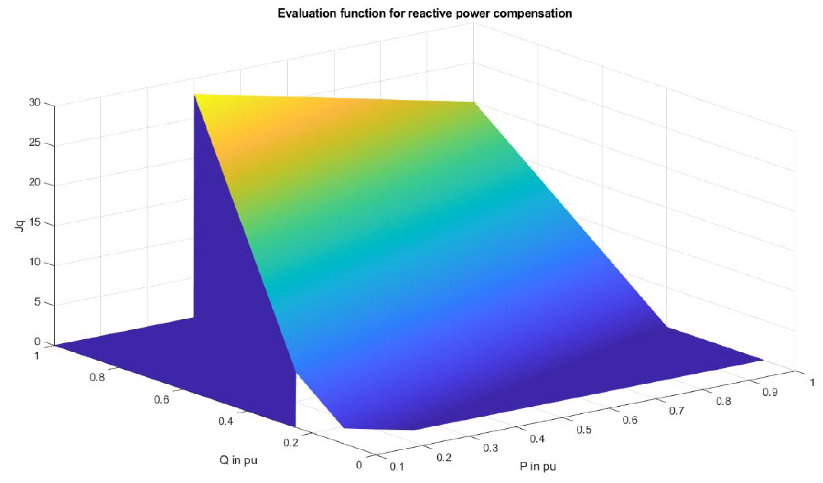
In practice, reactive power compensation is often required in power stations. For this reason, additional simulation data was generated for which high reactive power compensation will be required. For this reason, another set of input data was prepared for the simulation. However, in this case, we have a problem of multi-criteria optimization. The reactive power at the node and the RMS voltage are strongly related.

3.2. Results of Simulation Research Using Power Flow Calculations in Power Network with High Reactive Power Consumption

The simulation tests were carried out in two variants. Application of an evolutionary algorithm to optimize voltage regulation. Then, the required number of connected capacitor banks was determined, and after such a change, the flow calculations were performed again.

Table 5. The minimum and maximum number of required capacitor banks of 30 KVar for voltage regulation with an evolutionary algorithm in high reactive consumption.

Minimum Capacitor Qmin	Maximum Capacitor Qmax	Average Capacitor Qavg
0	170	54

shows the minimum, maximum and average number of capacitor banks required. Therefore, the reactive power compensation system should be designed for at least 170 capacitor banks. It was assumed that the reactive power compensation system would be able to switch on capacitor banks every 30 KVar with a maximum number of Q_max = 200.

Table 6. Influence of independent reactive power compensation on the quality of voltage regulation.

The Number of the Second Dataset	Number of Times Reactive Power Compensation Was Required	Number of Cases Where the Voltage Quality Deteriorated Due to Reactive Power Compensation
6399	6368	4638

and

Table 7. Influence of independent reactive power compensation on the quality of voltage regulation—one case.

Node No	Voltage Value before Compensation in p.u.	Voltage Value after Compensation in p.u.
3	1.129	1.191
4	1.037	1.107
5	0.990	1.064
6	0.962	1.038
7	0.943	1.021
8	1.074	1.140
9	1.047	1.116
10	1.031	1.101
11	1.015	1.087
12	1.043	1.112
13	1.000	1.073
14	0.974	1.050
15	0.955	1.032

present the results of the reactive power compensation influence on the voltage quality.

Implemented independently of the reactive power compensation voltage regulation, it decreased the evaluation function in 73% of cases. It follows that the reactive power compensation should be an element of the integrated voltage and reactive power regulation system (Table 6).

When the voltage is close to the upper allowable limit, connecting the capacitor banks additionally causes its increase, which results in deterioration of the quality of voltage regulation (Table 7).

3.3. Results of Simulation Research Using Power Flow Calculations in Pareto Multi-Criteria Optimizing

One of the solutions is presented below (

Table 8. The result of two-criteria optimization with the indicator of the quality of regulation.

No	OLTC Position	Number Capacitor	J	JQ	e_max—Maximum Absolute Value of Voltage Error for the Entire Network	|tg φ|
1	13	4	0.5	85.4	0.1113	0.74
2	14	26	0.5	61.7	0.113	0.64
3	15	48	0.5	38.3	0.1129	0.55
4	21	181	0.5	0	0.113	0.011

). Out of 8200 possible solutions, the two-criteria optimization algorithm chose four (see Figure 18). Then the Pareto-front solution selection algorithm chose solution no 4.

Then, the results of three simulations were compared for a dataset with high reactive power demand. The first one was carried out with the help of an evolutionary algorithm—single-criterion optimization. The second one, using the results from the first one, uses the classic algorithm for reactive power compensation. The last one was carried out with the use of two-criteria optimization (see

Table 9. The minimum and maximum value of the voltage error for different voltage regulation versions from the entire simulation.

Type of Voltage Regulation	Minimal Voltage Deviation in p.u.	Maximal Voltage Deviation in p.u.
Voltage regulation with an evolutionary algorithm	−0.15	0.41
Voltage regulation with an evolutionary algorithm and independent compensation of reactive power	−0.21	0.22
With the use of two-criteria optimization and the Pareto-front solution selection algorithm	−0.14	0.12

and

Table 10. The minimum and maximum value of the |tgφ| for different voltage regulation versions from the entire simulation.

Type of Voltage Regulation	Minimal |tgφ|	Maximal |tgφ|
Voltage regulation with an evolutionary algorithm	0.32	0.92
Voltage regulation with an evolutionary algorithm and independent compensation of reactive power	0	0.52
With the use of two-criteria optimization and the Pareto-front solution selection algorithm	0	0.4

).

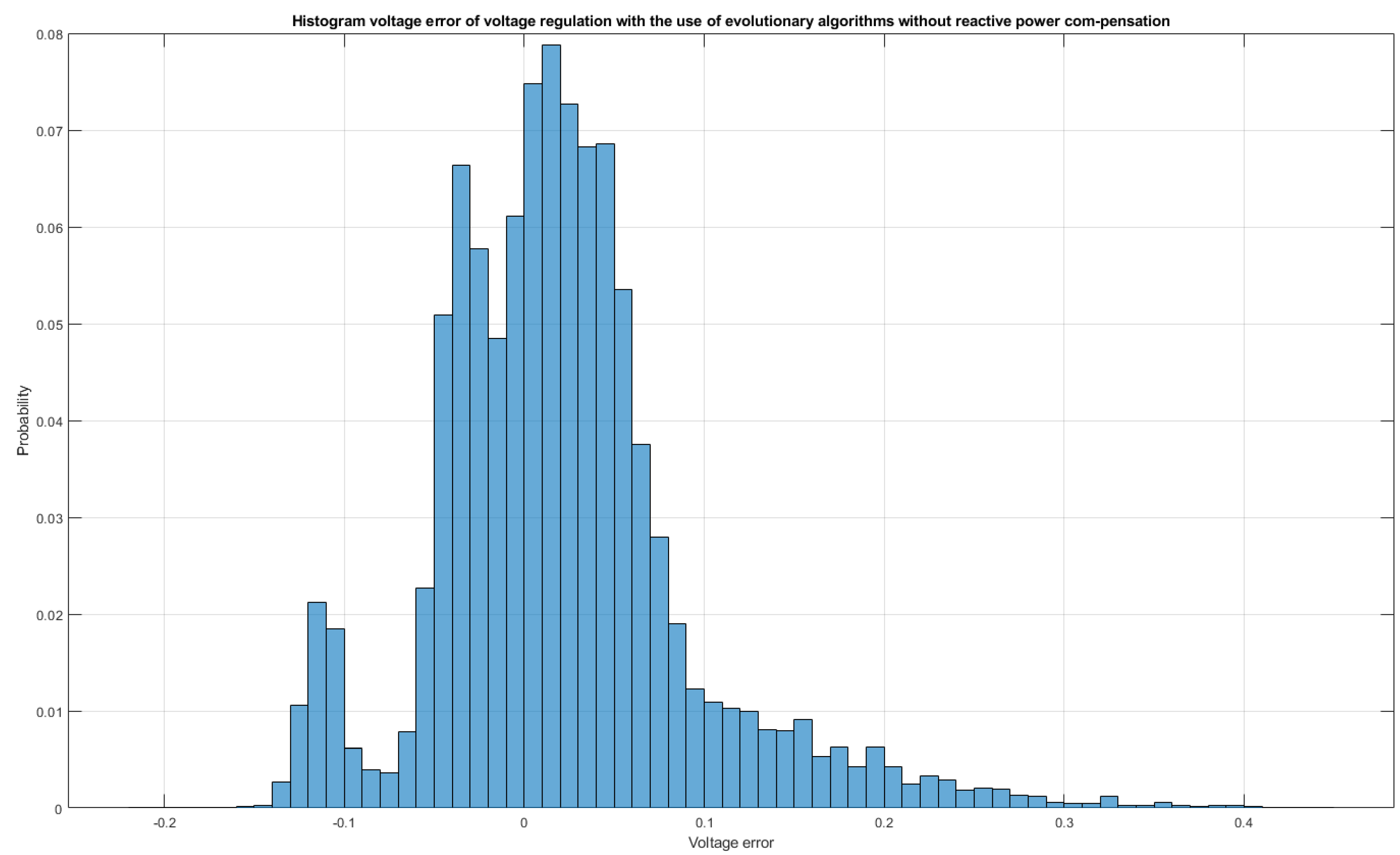
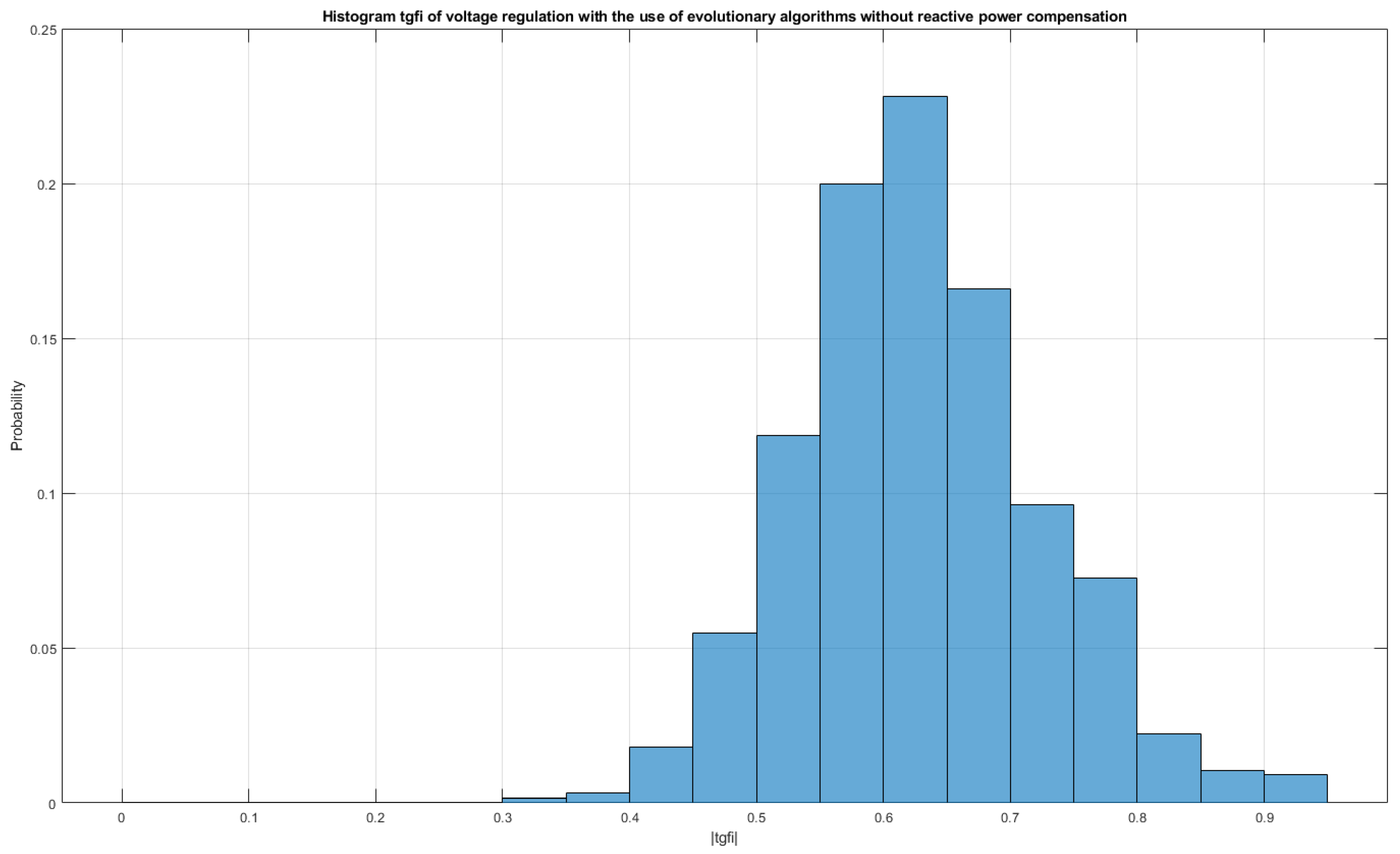
In the case of voltage regulation with the use of evolutionary algorithms without reactive power compensation, there are large positive voltage errors. The maximum tgφ factor significantly exceeds the permissible value. In the case of voltage regulation using evolutionary algorithms with independent reactive power compensation, the tgφ range has improved, but it also exceeds the allowable value. The voltage deviations range from ±20% of Un. Only the reaction with multi-criteria optimization keeps the tgφ in the correct range. The range of voltage deviations slightly exceeds the permissible value by a maximum of 4% Un.

The first three figures show the frequency distribution of the voltage error. Figure 19 shows the voltage error for the evolution algorithm. The next Figure 20 shows the voltage error for the evolution algorithm with independent reactive power compensation. Figure 21 shows the voltage deviation for two-criteria optimization and the algorithm for selecting the Pareto front solution. For multi-criteria optimization, the obtained values were the smallest range of voltage errors and the highest frequency of errors close to zero. The charts above show that multi-criteria optimization works best. The next three figures refer to the absolute value of the tgφ coefficient. Figure 22 shows the results of optimization of the evolution algorithm. The next Figure 23 shows tgφ and the evolution algorithm with independent reactive power compensation. Figure 24 shows the tgφ for two-criteria optimization and the algorithm for selecting a Pareto front solution. Only for the multi-criteria algorithm, the results of the tgφ coefficient were obtained within the acceptable range.

4. Discussion and Conclusions

The use of voltage measurements from all MV/LV substations and the use of evolutionary algorithms significantly improve the quality of voltage regulation. Despite voltage changes in the reference node and power changes in load nodes, the voltage variance is several dozen smaller than in the case of classical regulation. The voltage range in nodes with the use of evolutionary algorithms has higher values than in the case of classical regulation. This is justified as there are greater voltage drops in distant nodes when there are no local energy sources. When analyzing the minimum and maximum values for the three control variants, it is clear that in the case of no regulation, these values are outside the range of permissible values. In the case of classical regulation, there was an improvement. It is true that the minimum values exceed the lower limit of the permissible voltage range. Only the results obtained using the evolutionary algorithm with access to the current measurement values of the network nodes allowed for a significant improvement in the quality of voltage regulation.

Independently conducted voltage regulation and reactive power compensation often cause deterioration of one of them. This is due to the fact that if the voltage on the MV side is close to the upper allowable limit and reactive power compensation is required, then the voltage value increases above the limit. For a data set with a higher reactive power, there were as many as 73% of such cases. Typically, reactive power compensation systems switch off all capacitor banks after exceeding the upper voltage limit. However, this causes a deterioration of the work quality of the reactive power compensation system. Exceeding tgφ above 0.4 causes the necessity to pay additional charges, increase active power losses, and increase voltage drops. For this reason, it is required to build an integrated voltage regulation and reactive power compensation system. It follows that we have a multi-criteria optimization problem.

Classic voltage regulation systems in the power grid use only the transformer voltage on the lower voltage side. Due to the voltage drops at the ends of the lines, the voltage value may exceed the lower allowable limit. For this reason, current compensation was implemented in voltage regulators. However, there are many lines fed from the same transformer. These lines are loaded differently. These lines can also have different sections. Therefore, it is difficult to choose an impedance value for current compensation. In practice, current compensation is turned off and the voltage setpoint is set to a value between 1 and 1.1 p.u. In the case of a voltage regulation system that uses voltage measurements from all powered stations, the problem of current compensation does not exist. For this reason, it is recommended to build an integrated voltage regulation and reactive power compensation system using voltage measurements from all substations supplied from this transformer.

The use of multi-criteria optimization together with the Pareto-front solution selection algorithm allows to obtain the correct settings of the semiconductor on-load tap-changer and the correct number connected of capacitor banks.

The obtained results enable the construction of a voltage regulator and reactive power compensation in the form of a neural network, a fuzzy regulator, or a neuro-fuzzy regulator. The obtained results will be used to train the neural network. The exported Matlab results will be used in the Anaconda/Phyton environment to create a neural network. The resulting network will be implemented on an STM32 microcontroller using Cube.AI.

References

1. Choi, J.-H.; Moon, S.-I. The Dead Band Control of LTC Transformer at Distribution Substation. IEEE Trans. Power Syst. 2009, 24, 319–326. [Google Scholar] [CrossRef]
2. Choi, J.-H.; Kim, J.-C. Advanced voltage regulation method of power distribution systems interconnected with dispersed storage and generation systems. IEEE Trans. Power Deliv. 2001, 16, 329–334. [Google Scholar] [CrossRef]
3. Faiz, J.; Siahkolah, B. New Solid-State on-Load Tap-Changer Topology for Distribution Transformers. IEEE Power Eng. Rev. 2002, 22, 71. [Google Scholar] [CrossRef]
4. Patel, N.R.; Lokhande, M.M.; Jamnani, J.G. Solid-State on Load Tap-Changer for Transformer Using Microcontroller. Int. J. Eng. Dev. Res. 2014, 4, 101–104. [Google Scholar]
5. Demirci, O.; Torrey, D.A.; Degeneff, R.C.; Schaeffer, F.K.; Frazer, R.H. A new approach to solid-state on load tap changing transformers. IEEE Trans. Power Deliv. 1998, 13, 952–961. [Google Scholar] [CrossRef]
6. De Oliveira Quevedo, J.; Cazakevicius, F.E.; Beltrame, R.C.; Marchesan, T.B.; Michels, L.; Rech, C.; Schuch, L. Analysis and Design of an Electronic On-Load Tap Changer Distribution Transformer for Automatic Voltage Regulation. IEEE Trans. Ind. Electron. 2017, 64, 883–894. [Google Scholar] [CrossRef]
7. Korpikiewicz, J.G. A Concept of New Current Compensation in a HV/MV Transformer’s Semiconductor Tap-Changer Controller. Acta Energ. 2019, 17, 28–36. [Google Scholar]
8. Faiz, J.; Siahkolah, B. Electronic Tap-Changer for Distribution Transformers; Springer: Berlin/Heidelberg, Germany, 2011; Volume 2. [Google Scholar]
9. Sanjay, M.A.; Raosaheb, T.S.; Ravindra, N.S. Solid State on Load Tap Changer for Transformer. Resincap J. Sci. Eng. 2021, 5, 4. [Google Scholar]
10. Abdou, M.S.; Mostafa, H.E.; Abdalla, Y.S. Solid State-Based On-Load Tap-Changer Control. Port Said Eng. Res. J. 2013, 17, 79–84. [Google Scholar]
11. Faiz, J.; Siahkolah, B. Solid-state tap-changer of transformers: Design, control and implementation. Int. J. Electr. Power Energy Syst. 2011, 33, 210–218. [Google Scholar] [CrossRef]
12. Shi, F.; Yin, Y.; Ding, B.P.; Gao, F.; Jia, P.F.; Hao, L.N.; Zhang, L. Development of 110 kV Thyristor Assisted Arc Extinguishing Hybrid OLTC. E3S Web Conf. 2021, 243, 01003. [Google Scholar] [CrossRef]
13. Faiz, J.; Siahkolah, B. Differences Between Conventional and Electronic Tap-Changers and Modifications of Controller. IEEE Trans. Power Deliv. 2006, 21, 1342–1349. [Google Scholar] [CrossRef]
14. Korpikiewicz, J.G.; Mysiak, P. Classical and Solid-state Tap-changers of HV/MV Regulating Transformers and their Regulators. Acta Energ. 2017, 14, 110–117. [Google Scholar]
15. Wei, T.; Yu, Z.; Chen, Z.; Zhang, X.; Wen, W.; Huang, Y.; Zeng, R. Design and test of the bidirectional solid-state switch for an 160 kV/9kA hybrid DC circuit breaker. In Proceedings of the 2018 IEEE Applied Power Electronics Conference and Exposition (APEC), San Antonio, TX, USA, 4–8 March 2018; pp. 141–148. [Google Scholar] [CrossRef]
16. Su, X.; Liu, J.; Tian, S.; Ling, P.; Fu, Y.; Wei, S.; SiMa, C. A Multi-Stage Coordinated Volt-Var Optimization for Integrated and Unbalanced Radial Distribution Networks. Energies 2020, 13, 4877. [Google Scholar] [CrossRef]
17. Beyer, K.; Beckmann, R.; Geißendörfer, S.; von Maydell, K.; Agert, C. Adaptive Online-Learning Volt-Var Control for Smart Inverters Using Deep Reinforcement Learning. Energies 2021, 14, 1991. [Google Scholar] [CrossRef]
18. Gubert, T.C.; Colet, A.; Casals, L.C.; Corchero, C.; Domínguez-García, J.L.; Sotomayor AA, D.; Alet, P.J. Adaptive Volt-Var Control Algorithm to Grid Strength and PV Inverter Characteristics. Sustainability 2021, 13, 4459. [Google Scholar] [CrossRef]
19. Jung, Y.; Han, C.; Lee, D.; Song, S.; Jang, G. Adaptive Volt–Var Control in Smart PV Inverter for Mitigating Voltage Unbalance at PCC Using Multiagent Deep Reinforcement Learning. Appl. Sci. 2021, 11, 8979. [Google Scholar] [CrossRef]
20. Go, S.-I.; Yun, S.-Y.; Ahn, S.-J.; Kim, H.-W.; Choi, J.-H. Heuristic Coordinated Voltage Control Schemes in Distribution Network with Distributed Generations. Energies 2020, 13, 2849. [Google Scholar] [CrossRef]
21. Hasan, E.O.; Hatata, A.Y.; Badran, E.A.; Yossef, F.M.H. A new strategy based on ANN for controlling the electronic on-load tap changer. Int. Trans. Electr. Energ. Syst. 2019, 29, e12069. [Google Scholar] [CrossRef]
22. Keshta, H.E.; Ali, A.A.; Malik, O.P.; Saied, E.M.; Bendary, F.M. Voltage Control of Islanded Hybrid Micro-grids Using AI Technique. In Proceedings of the 2020 IEEE Electric Power and Energy Conference (EPEC), Edmonton, AB, Canada, 9–10 November 2020; pp. 1–6. [Google Scholar] [CrossRef]
23. Bielecka, A.; Wojciechowski, D. Predykcyjne sterowanie równoleg\lym filtrem aktywnym ze sprzężeniem od prądu zasilającego. Przegląd Elektrotechniczny 2019, 128–132. [Google Scholar] [CrossRef]
24. Bielecka, A.; Wojciechowski, D. Stability Analysis of Shunt Active Power Filter with Predictive Closed-Loop Control of Supply Current. Energies 2021, 14, 2208. [Google Scholar] [CrossRef]
25. Strzelecki, R.; Mysiak, P.; Sak, T. Solutions of inverter systems in Shore-to-Ship Power supply systems. In Proceedings of the 2015 9th International Conference on Compatibility and Power Electronics (CPE), Lisbon, Portugal, 24–26 June 2015; pp. 454–461. [Google Scholar]
26. Shuttleworth, R.; Tian, X.; Fan, C.; Power, A. New tap changing scheme. IEE Proc. Electr. Power Appl. 1996, 143, 108–112. [Google Scholar] [CrossRef]
27. Lebkowski, A. Evolutionary methods in the management of vessel traffic. In Information, Communication and Environment: Marine Navigation and Safety of Sea Transportation; CRC Press: Boca Raton, FL, USA, 2015; pp. 259–266. [Google Scholar]
28. Fadaee, M.; Radzi, M.A.M. Multi-objective optimization of a stand-alone hybrid renewable energy system by using evolutionary algorithms: A review. Renew. Sustain. Energy Rev. 2012, 16, 3364–3369. [Google Scholar] [CrossRef]
29. Gu, F.; Liu, H.-L.; Tan, K.C. A multiobjective evolutionary algorithm using dynamic weight design method. Int. J. Innov. Comput. Inf. Control 2012, 8, 3677–3688. [Google Scholar]
30. Lazarowska, A. Ant colony optimization based navigational decision support system. Procedia Comput. Sci. 2014, 35, 1013–1022. [Google Scholar] [CrossRef] [Green Version]
31. Lazarowska, A. Swarm intelligence approach to safe ship control. Pol. Marit. Res. 2015, 22, 34–40. [Google Scholar] [CrossRef] [Green Version]
Figure 1. Electromechanical tap-changer for power transformer from ABB [www.abb.com, accesed on 1 April 2020] (a), view of power transformer from ABB [www.abb.com, accesed on 1 April 2020] (b).
Energies 15 04773 g001
Figure 2. Schematic of the proposed electronic tap-changer [11].
Energies 15 04773 g002
Figure 3. Structure of the tested power network.
Energies 15 04773 g003
Figure 4. Structure of regulating winding for one phase.
Energies 15 04773 g004
Figure 5. Evaluation function for voltage node.
Energies 15 04773 g005
Figure 6. Evaluation function for reactive power compensation.
Energies 15 04773 g006
Figure 7. Algorithm for selecting one solution from the Pareto front.
Energies 15 04773 g007
Figure 8. Histogram of evaluation value—without voltage regulation and reactive power compensation.
Energies 15 04773 g008
Figure 9. Histogram of evaluation value—classic voltage regulation and without reactive power compensation.
Energies 15 04773 g009
Figure 10. Histogram of evaluation value—voltage regulation optimization by means of an evolutionary algorithm and without reactive power compensation.
Energies 15 04773 g010
Figure 11. Histogram of evaluation value—without voltage regulation and with reactive power compensation.
Energies 15 04773 g011
Figure 12. Histogram of evaluation value—classic voltage regulation and with reactive power compensation.
Energies 15 04773 g012
Figure 13. The voltage values for the network node no 4 for three control variants without reactive power compensation.
Energies 15 04773 g013
Figure 14. The voltage values for the network node no 7 for three control variants without reactive power compensation.
Energies 15 04773 g014
Figure 15. The voltage values for the network node no 11 for three control variants without reactive power compensation.
Energies 15 04773 g015
Figure 16. The voltage values for the network node no 13 for three control variants without reactive power compensation.
Energies 15 04773 g016
Figure 17. The voltage values for the network node no 15 for three control variants without reactive power compensation.
Energies 15 04773 g017
Figure 18. One of two-criteria optimization results.
Energies 15 04773 g018
Figure 19. Histogram voltage error—evolutionary algorithm.
Energies 15 04773 g019
Figure 20. Histogram voltage error—evolutionary algorithm with reactive power compensation.
Energies 15 04773 g020
Figure 21. Histogram voltage error—use of two-criteria optimization and the Pareto-front solution selection algorithm.
Energies 15 04773 g021
Figure 22. Histogram tgφ—evolutionary algorithm.
Energies 15 04773 g022
Figure 23. Histogram tgφ—evolutionary algorithm with reactive power compensation.
Energies 15 04773 g023
Figure 24. Histogram tgφ—use of two-criteria optimization and the Pareto-front solution selection algorithm.
Energies 15 04773 g024