Dispatch Optimization, System Design and Cost Benefit Analysis of a Nuclear Reactor with Molten Salt Thermal Storage

Abstract

Variable renewable energy availability has increased the volatility in energy prices in most markets. Nuclear power plants, with a large ratio of capital to variable costs, have historically operated as base load energy suppliers but the need for more flexible operation is increasing. We simulate the techno-economic performance of a 950 MW${}_t$ nuclear power plant, based on the Westinghouse lead-cooled fast reactor, coupled with molten salt thermal storage as a method for flexible energy dispatch. We use the System Advisor Model to model the nuclear reactor thermal power input and power cycle operating modes. We combine this robust engineering model with a mixed-integer linear program model for optimized dispatch scheduling. We then simulate the coupled nuclear and thermal storage system under different market scenarios with varying price volatility. We find that the coupled plant outperforms the base plant under markets where energy price peaks fluctuate by a factor of two or more about the mean price. We show that a calculated power purchase agreement price for the plant improves by up to 10% when operating under California energy market conditions. Sensitivity analysis on the thermal storage cost shows that the optimal design remains unchanged even when doubling costs.

1. Introduction

Nuclear power plants (NPP) have a high ratio of capital costs to variable costs which has historically made them a reliable option for baseload power supply under past energy market conditions. While NPPs have the ability to ramp production to load follow demand trends, the financial incentives are usually not enough to make this flexible operation viable with current technologies. As markets become more saturated with variable renewable energy (VRE) sources, market conditions become more volatile. Solar energy supplies the grid with power during daylight hours; however, demand peaks during early morning and late afternoon hours. Solar availability and grid demand peak out-of-phase, which widens the range of wholesale energy prices throughout the day. Prices during the middle of the day are known to reach negative values in VRE-saturated markets like the California Independent System Operator market (CAISO) in the western United States. They, however, increase rapidly when demand spikes in the evening as residential load comes online and the previously abundant solar power wanes [1].

High pricing periods can be lucrative for power plants with the right capacity and ramping capabilities. Natural gas plants perform particularly well in these markets during periods of rapid power ramping with their low operating costs and recent, historically low natural gas prices. Comparatively, nuclear plant operating costs do not vary with production as dramatically and rarely shut down outside of planned refueling outages. They need to pay off their high capital costs as quickly as possible and therefore are generally incentivized to operate at full power whenever possible, including in the middle of the day when prices are unfavorable. Flexible operation of nuclear power is therefore of growing importance for both current and advanced nuclear technologies [2,3,4,5,6,7,8,9].

One possible technology to help nuclear operate more flexibly is thermal energy storage (TES). This allows the nuclear plant to maintain constant thermal output while reducing its electrical output during low or even negative pricing periods by the added option to store its thermal energy. Then, during high pricing periods, the nuclear plant can sell its own constant thermal output as well as the excess stored energy. Adding TES to an existing nuclear plant design would require over-sizing the turbine, generator, and supporting subsystems relative to the originally intended nuclear thermal output to provide extra capacity that can be dispatched during periods of high demand. This would predictably increase capital costs and push the power cycle to perform at lower efficiencies during charging periods. However, these costs can be offset against enhanced revenue from optimized dispatch.

In this paper, we develop a model to investigate the techno-economic performance of a nuclear plant coupled with thermal energy storage, specifically using two tanks of molten salt as used in concentrating solar power (CSP) systems and increasingly of interest for nuclear reactors. Our model uses the Westinghouse Lead-cooled Fast Reactor (LFR) as a baseline for the nuclear plant model [10,11]; the thermal storage is assumed to be a two-tank storage system with molten salt (60% NaNO${}_3$, 40% KNO${}_3$) as the thermal fluid. Our starting point is the engineering model of a CSP system in the System Advisor Model (SAM) provided by the National Renewable Energy Laboratory [12]. Here we modify this model for the case of a nuclear reactor with the two-tank molten salt TES, specifically to determine the thermodynamics of the full system at every timestep. A mixed-integer linear program is used to generate optimized energy dispatch schedules to be used as targets for the SAM engineering model. We investigate the effects of over-sizing the turbine of a steam Rankine cycle on the overall revenue of the plant and use this to determine optimal turbine and tank sizing for a nuclear plant. We ultimately develop a modeling capability to analyze such systems, and apply this to derive useful insight into the overall cost-benefit of molten salt TES for nuclear reactors under various pricing scenarios.

2. Methods

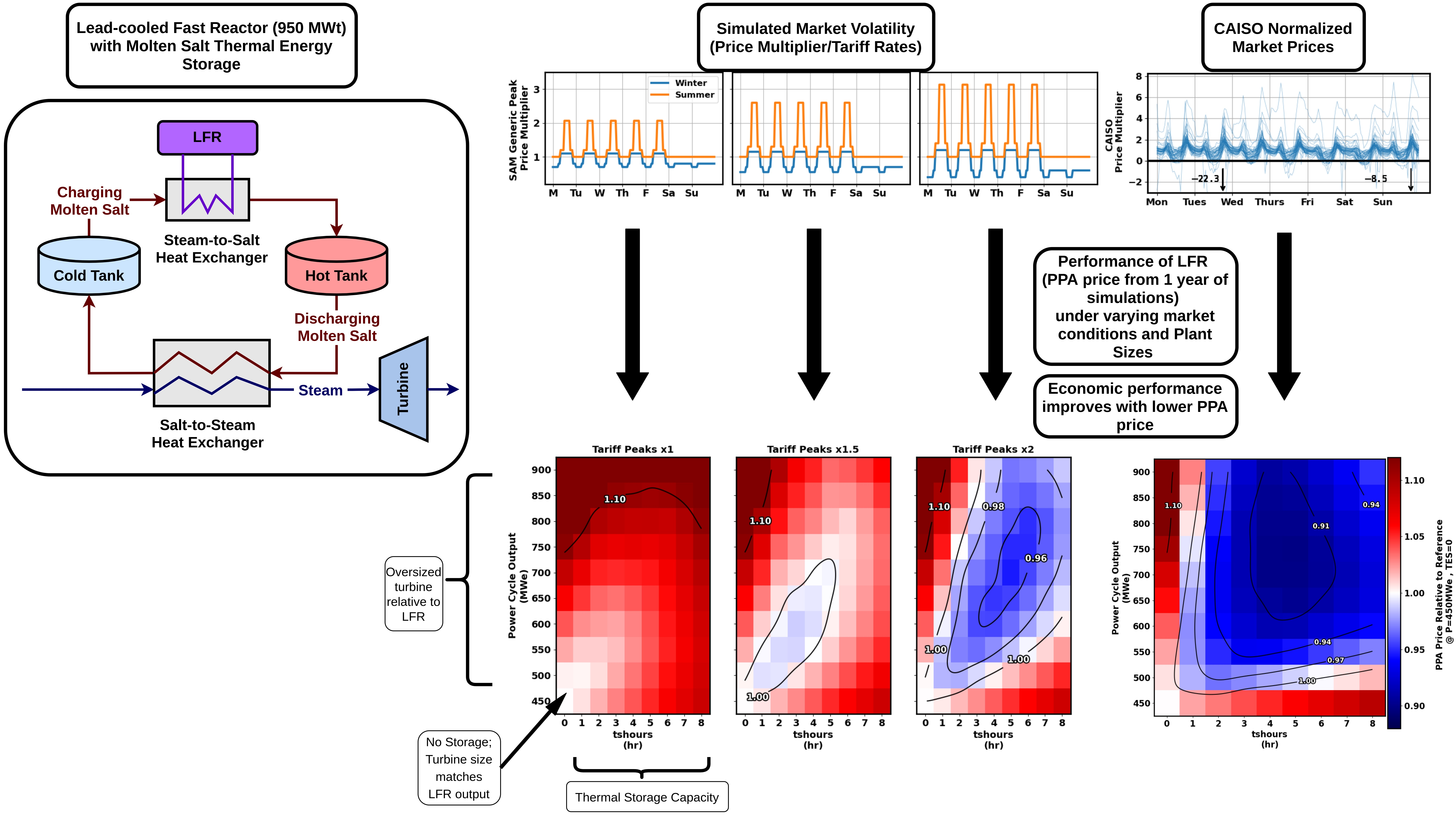
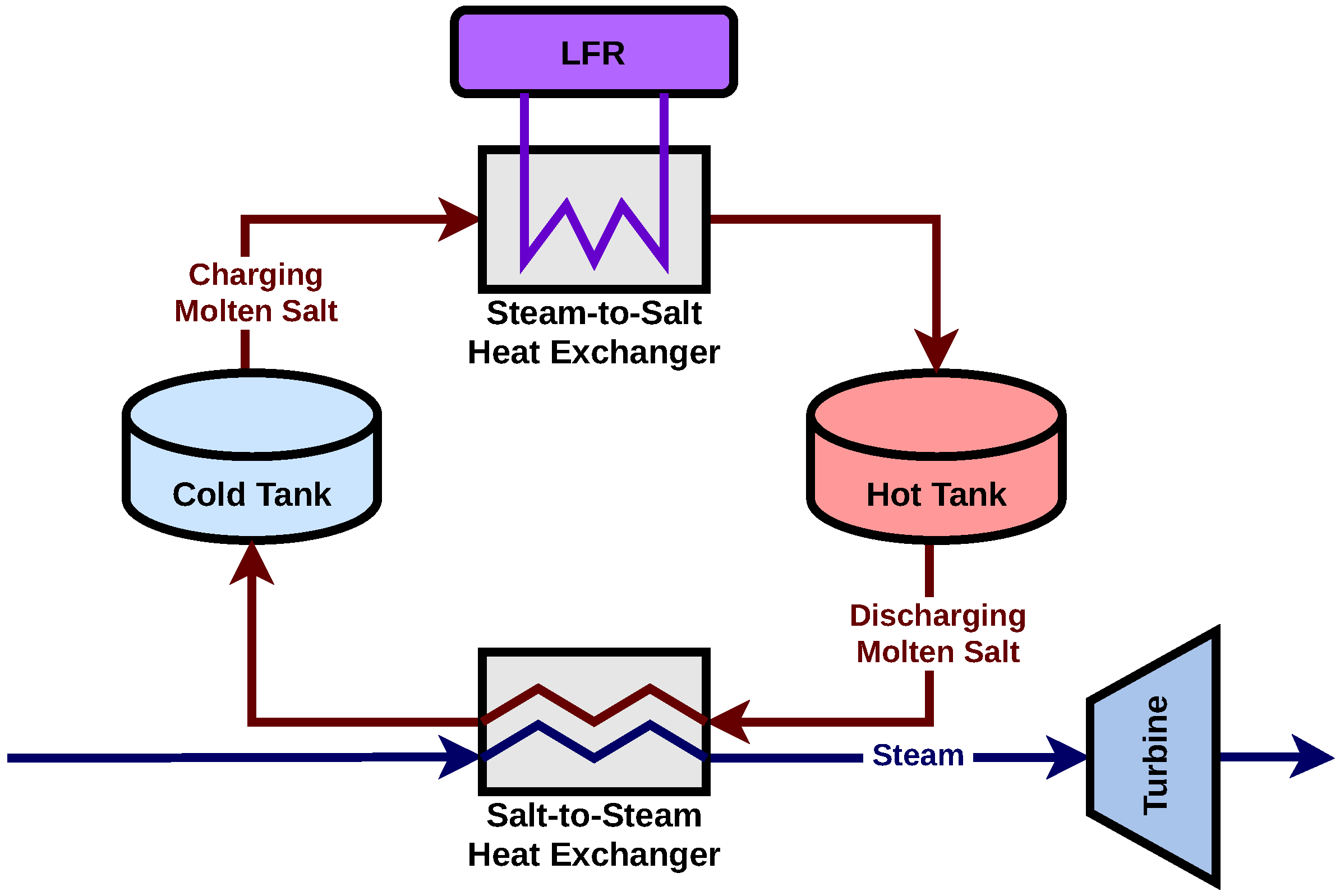
2.1. Reactor and Plant Assumptions

We modeled a nuclear reactor with nominal thermal output of 950 ${\mathrm{MW}}_t$. We used a direct charging model for the TES as shown in the schematic in Figure 1. During the charging phase, a mass flow of molten salt was drawn from the cold tank and heated via heat exchange with the nuclear plant (using a secondary loop with the power cycle working fluid). The heated molten salt was then routed to the hot tank for storage. The discharging phase becomes the primary mode for adding heat to the power cycle—mass flow was drawn from the hot tank and heated the steam via direct heat exchanger before the steam entered the turbine. The cooled molten salt was then stored in the cold tank for later use in charging. The thermal storage could also be operated in a balanced mode if no charging or discharging was desired—that is, the mass flow out of the cold tank matches mass flow out of the hot tank to balance heat addition from the nuclear plant.

Our nuclear reactor design was modeled after the Westinghouse LFR plant. Lead-cooled fast reactors are an advanced reactor concept being developed currently in the US [11,13], Russia [14], and Belgium [15]. We chose the LFR within this study for many of its safety and performance advantages [16,17,18] including but not limited to:

• better fuel utilization, lower waste production, and the capability to operate at higher temperatures with fast neutron spectrum operation;
• ability to operate coolant at atmospheric pressure with more compact infrastructure; and 
• inherent safety mechanics due to high thermal inertia from thermal capacity and larger coolant mass, as well as retention of radioactive isotopes by lead in case of severe accident.

These advantages also lower the capital costs of the plant, making it economically competitive among other advanced reactor designs and a fitting candidate for further revenue accumulation with a coupled TES system. Current designs use an outlet coolant temperature of up to about 570 °C; the reactor is capable of higher temperatures but is limited by material properties of the piping infrastructure. These outlet temperatures match the highest operating temperatures, around 560 °C, of the molten salt [7,19].

The Westinghouse design utilizes either a direct supercritical CO${}_2$ (sCO${}_2$) power cycle, or, more recently, supercritical Rankine cycle to produce electricity. As it is undesirable to change the working fluid of the in-vessel heat exchangers, the TES must be integrated into the system via an sCO${}_2$-to-salt or supercritical steam-to-salt heat exchanger. The stored thermal energy can then be dispatched through a salt-to-sCO${}_2$ or salt-to-supercritical steam heat exchanger. Such a configuration was recently analyzed in Ref. [20] for the case of sCO₂, confirming that the configuration is viable. It is also possible to configure a supercritical Rankine cycle in this manner, and analysis of this is ongoing at the University of Wisconsin–Madison. Indirect charging of the TES in this manner will naturally incur a ‘round trip’ efficiency penalty, which will somewhat penalize the desirability of the TES. However, the efficiency of the cycle at the design point is unaffected by the presence of the TES as the heat is transferred directly from the lead to the working fluid.

In this work, we assumed an alternative configuration also being investigated by the advanced reactor community: to integrate the TES loop between the primary heat transfer fluid and the working fluid before it enters the turbine. For a nuclear reactor, this typically increases the number of loops required to transfer the heat to the power conversion cycle (i.e., adds an extra heat exchanger) and hence introduces a thermodynamic penalty regardless of whether the TES is being charged or discharged, rather than a ‘round trip’ penalty. The intermediate working fluid loop between the lead primary and molten salt tertiary also alleviates safety concerns from any potential lead–salt interactions. This moves away from the Westinghouse configuration that explores indirect charging, which can extract power from the secondary working fluid loop before charging the TES with potential improvement in net efficiency, but is still a useful model to derive insights and trends and allows the ability to draw more generalizable conclusions. Moreover, future work is planned to investigate the indirect TES configuration. Here, we do not generally include a cost penalty for the thermodynamic inefficiencies of integrating the TES with the nuclear reactor in the interests of simplicity. As a sensitivity case, we do however introduce a cost penalty through a reduction in the design point thermodynamic efficiency (as is the case if the nuclear reactor charges the TES directly) for cases where a TES is included, relative to the reference case where a TES is not included. A round-trip efficiency penalty to using the TES (as is the case if the nuclear reactor charges the TES indirectly) is not considered here as it is too complicated to treat accurately without altering the underlying engineering models, which is in progress and will be included in future work.

We used several models with varying levels of fidelity to represent the system portrayed in Figure 1: a dispatch model to generate optimal operating schedules for all subsystems and an engineering model in SAM to resolve thermodynamic and energy balances for the full plant at each simulation time step. The SAM model utilizes tabulated data of the power conversion cycle for design and off-design performance. This power conversion cycle data typically comes from detailed thermodynamic calculations of the power conversion cycle. The time constant of the power conversion cycle is typically much less than the simulation timestep and therefore a steady-state off-design calculation is acceptable. Here, we assume a steam Rankine cycle design as the baseline model for our power cycle to make our results more generalizable. We utilize the model from Ref. [21], written in Engineering Equation Solver (EES) to generate our off-design data [22]. Tabular data within SAM are also normalized to make the model more generalizable.

Within our engineering model, we adopt a simple representation of LFR operations. On the reactor side of the steam-to-salt heat exchanger in Figure 1, we assume that the LFR can vary its control rod insertion as well as primary loop mass flow to alter thermal power output. We do not directly model these complex nonlinear operations but rather their end results: the LFR outputs its set-point 950 ${\mathrm{MW}}_t$ thermal output and, when needed, can reduce power to a desired fraction of the nominal production. The subtleties of the operation to achieve this outcome are not directly represented in the scope of this work, but as with the steam cycle, the time constant of the LFR is sufficiently short relative to the timestep of the TES that we can model such behavior through simple constraints on ramping.

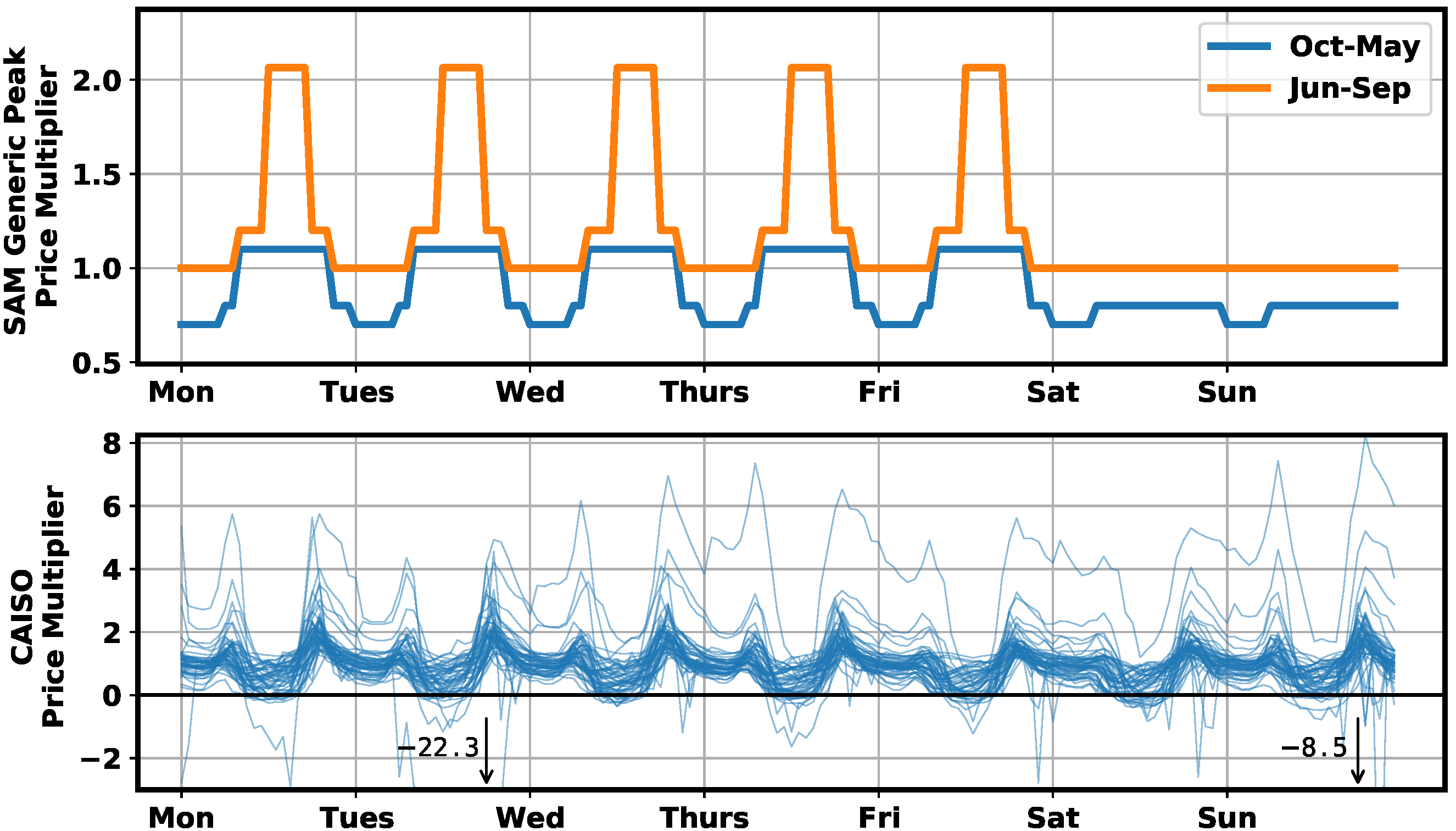
2.2. Market Pricing and Economic Structure

We evaluate the effect of coupling TES with an LFR by simulating performance over a full year under varying market conditions. We represent market conditions through the use of a tariff rate, or price multiplier, as a time series—this is a normalized factor representing relative pricing throughout the year as shown in Figure 2. We therefore assume that the power plant is a price taker. This is a useful simplifying assumption as the dynamic behavior of energy markets is highly complex, and in this manner we isolate the dispatch optimization of the power plant from bidding behavior; the tariff rate therefore captures the variance in clearing prices within the purported wholesale energy market. Such an approach is typical for CSP plants [23]. We also assume perfect price forecasting. This is a useful simplifying assumption as price forecasting is also highly complex, and it has been shown that it is possible to take into account imperfect knowledge through additional constraints, e.g., through holding some of the TES capacity in reserve [24].

We use two separate tariff rate time series to evaluate plant performance—a generic peak pricing schedule from SAM and a normalized pricing time series from CAISO data—as shown in Figure 2. The SAM tariffs represent a single price peak during the day and lower prices at night; all multipliers are normalized so that they integrate over a full year to 8760 (an hourly average of 1.0) and therefore do not artificially inflate the revenue over the simulation. The price peaks are set higher during the weekdays than weekends; there is also an increase in price during the summer relative to winter months. The SAM tariffs are not meant to mimic any current market or specific geographic region, rather they are meant to present a simple way to test both daily and seasonal plant responses to price ramping. The CAISO tariff rates in the bottom of Figure 2 were generated using collected data from the online OASIS tool [25]. These are locational marginal prices (LMP) for the Iron Mountain (IRONMTN_2_N001) node taken from 1 January to 31 December of 2019. The LMP are normalized in the same way as the SAM tariffs to not artificially inflate revenue values. Figure 2 shows weekly pricing curves from the CAISO data throughout the entire year. Prices range over more dramatic peaks compared to the SAM tariffs, with the added feature that they sometimes drop to negative values when excessive VRE is available and the Independent System Operators (ISOs) want to penalize further addition to the grid. A daily pattern with early morning and late afternoon peaks is evident from the normalized data.

The economic performance of the coupled LFR and TES system is evaluated using SAM financial modules with the previous tariff rate schedules and a simulated power generation schedule to calculate a power purchase agreement (PPA) price for the site. The PPA price represents a minimum wholesale price of energy at which a power plant should sell its energy to the grid, taking into account both capital and O&M costs. It is calculated by assuming a desired internal rate of return for the initial plant investment and a specified return time—the PPA price would then present the minimum price the plant should sell its produced electricity to, say, make back 11% return in 20 years. For our purposes, the objective of a low PPA prices makes the plant more competitive in the market while still guaranteeing a return on the initial capital investment.

The cost structure of the plant is calculated by assuming some nominal values and using data from our partners at Westinghouse, shown in

Table 1. Costs and other parameters used for evaluating plant economic performance.

Symbol	Value	Units	Description	Source
Dispatch Optimization Parameters
$C^{pc}$	0.00875	$\$/{\mathrm{kW}}_e·\mathrm{h}$	Operating cost of power cycle	Scaled SAM parameters [23,26,27]
$C^{csu}$	27,345	$\$/\mathrm{start}$	Penalty for power cycle cold start-up	“1
$C^{chsp}$	5470	$\$/\mathrm{start}$	Penalty for power cycle hot start-up	“
$C^{csb}$	0.00175	$\$/{\mathrm{kW}}_t·\mathrm{h}$	Operating cost of power cycle standby operation	“
$C^{{\Delta }_w}$	0.04375	$\$/\Delta {\mathrm{kW}}_e$	Penalty for power cycle production change	“
$C^{v_w}$	1.75	$\$/\Delta {\mathrm{kW}}_e$	Penalty for power cycle production change past design	“
$C^{nop}$	0.00734	$\$/{\mathrm{kW}}_t·\mathrm{h}$	Operating cost of nuclear plant	Westinghouse estimates
Engineering Model Financial Parameters
$r^{fin}$	7	%	Interest rate on financing loan	General assumption
${\tau }^{con}$	4	yr	Construction time	“
$C^{tes}$	29.8	$\$/{\mathrm{kW}}_t·\mathrm{h}$	Thermal energy storage cost	Scaled SAM parameters [23,26,27]
$C^{nuc}$	4150	$\$/{\mathrm{kW}}_e·\mathrm{h}$	Nuclear plant cost including fuel over analysis period	Westinghouse estimates

¹ Tables elements annotated with (“) are equivalent to the element in the row above.

. We have outlined the calculation of extra capital costs incurred from oversizing the turbine relative to the thermal output. First, we define a reference electrical output from the nuclear thermal output design point as:

$$W^{n,des}={\eta }^{des}{\dot{Q}}^{n,des},$$

(1)

where ${\eta }^{des}$ is the power cycle efficiency at the design point and ${\dot{Q}}^{n,des}$ is the design point nuclear thermal output of 950 ${\mathrm{MW}}_t$. We then calculate the cost associated with the oversized turbine by the following:

$$C^{n,des+}=\frac{C^{nuc}{W}^{n,des}+C^{turb+}(W^{pc+}-W^{n,des})}{W^{pc+}},$$

(2)

where $C^{n,des+}$ is the cost of the nuclear plant over the design point and $W^{pc+}$ is the electric power output of the over-sized cycle being considered. The parameter $C^{nuc}$ is given in Table 1; $C^{turb+}$ is the cost of additional power cycle capacity above the nominal turbine output, given as a cubic approximation in Figure 3 from our partners at Westinghouse. We similarly calculate a thermal storage cost as:

$$C^{tes+}=W^{pc+}{T}^{tes}{C}^{tes},$$

(3)

where $T^{tes}$ is the amount of storage in the molten salt tanks given in equivalent full-load hours of the power cycle output, $C^{tes}$ is the per-unit cost of TES, and $C^{tes+}$ is the total cost of TES at the given capacity. TES and LFR capital costs are both updated as input parameters for the financial portion of the SAM engineering model to calculate PPA price. Financing costs during the construction period are also adjusted to be consisted with the updated plant capital cost.

2.3. Mathematical Formulation of Dispatch Optimization Problem

With the market pricing data shown in Figure 2, we can simulate plant performance under differing market conditions. Plant operating schedules for a given day would need to be optimized to dispatch energy according to some economically advantageous strategy. We implement an optimization scheme to generate optimal energy dispatch schedules for the plant using a mixed-integer linear programming (MILP) paradigm developed from Wagner et al. [23] and Cox et al. [27]. The problem is first formulated using Pyomo [28] to create an optimization model by calculating the initial operating state of the nuclear plant, power cycle, and molten salt tank subsystems. Upper and lower bounds are also used to constrain ramping within the time steps of the time horizon. Other parameters include the tariff rate $P_t$ for each time step of the time horizon $\mathcal{T}$, as well as cycle efficiency adjustments due to ambient temperature, all listed in

Table 2. Parameters used for dispatch optimization.

Symbol	Units	Description
Sets
$\mathcal{T}$		Set of all time steps within time horizon
Time-Indexed Parameters
$Q_t^{in,nuc}$	${\mathrm{kW}}_t$	Available thermal power generated by the nuclear plant in time t
${\delta }_t^{ns}$	-	Estimated fraction of time t required for nuclear start-up
${\eta }_t^{amb}$	-	Cycle efficiency ambient temperature adjustment factor in time t
${\eta }_t^c$	-	Normalized condenser parasitic loss in time t
$P_t$	$\$/{\mathrm{kW}}_e·\mathrm{h}$	Electricity sales price in time t
$Q_t^c$	${\mathrm{kW}}_t$	Allowable power per period for cycle start-up in time t
$W_t^{u+}$	${\mathrm{kW}}_e$	Maximum power production when starting generation in time t
$W_t^{u-}$	${\mathrm{kW}}_e$	Maximum power production in time t when stopping generation in time $t+1$
Steady-State Parameters
$\alpha$	$	Conversion factor between unitless and monetary values
$E^c$	${\mathrm{kW}}_t·\mathrm{h}$	Required energy expended to start cycle
${\eta }^{des}$	-	Cycle nominal efficiency
$E^u$	${\mathrm{kW}}_t·\mathrm{h}$	Thermal energy storage capacity
${\eta }^p$	${\mathrm{kW}}_e/{\mathrm{kW}}_t$	Slope of linear approximation of power cycle performance curve
$L^c$	${\mathrm{kW}}_e/{\mathrm{kW}}_t$	Cycle heat transfer fluid pumping power per unit energy expended
$Q^b$	${\mathrm{kW}}_t$	Cycle standby thermal power consumption per period
$Q^l$	${\mathrm{kW}}_t$	Minimum operational thermal power input to cycle
$Q^u$	${\mathrm{kW}}_t$	Cycle thermal power capacity
$W^b$	${\mathrm{kW}}_e$	Power cycle standby operation parasitic load
${\dot{W}}^l$	${\mathrm{kW}}_e$	Minimum cycle electric power output
${\dot{W}}^u$	${\mathrm{kW}}_e$	Cycle electric power rated capacity
$W^{\Delta +}$	${\mathrm{kW}}_e/\mathrm{h}$	Power cycle ramp-up designed limit
$W^{\Delta -}$	${\mathrm{kW}}_e/\mathrm{h}$	Power cycle ramp-down designed limit
$W^{v+}$	${\mathrm{kW}}_e/\mathrm{h}$	Power cycle ramp-up violation limit
$W^{v-}$	${\mathrm{kW}}_e/\mathrm{h}$	Power cycle ramp-down violation limit
${\delta }^{nl}$	h	Minimum time to start the nuclear plant
$E^n$	${\mathrm{kW}}_t·\mathrm{h}$	Required energy expended to start nuclear plant
$L^n$	${\mathrm{kW}}_e/{\mathrm{kW}}_t$	Nuclear pumping power per unit power produced
$Q^{nl}$	${\mathrm{kW}}_t·\mathrm{h}$	Minimum operational thermal power delivered by nuclear
$Q^{nsb}$	${\mathrm{kW}}_t·\mathrm{h}$	Required thermal power for nuclear standby
$Q^{nsd}$	${\mathrm{kW}}_t·\mathrm{h}$	Required thermal power for nuclear shut down
$Q^{nu}$	${\mathrm{kW}}_t·\mathrm{h}$	Allowable power per period for nuclear start-up
$W^{nht}$	${\mathrm{kW}}_e·\mathrm{h}$	Nuclear piping heat trace parasitic loss

. Variables for the MILP are classified as either continuous or binary variables. Continuous variables represent power generation quantities for the various subsystems (e.g., the power cycle electric output, nuclear thermal generation, thermal tank stored energy) for each time step in $\mathcal{T}$; the binary variables are decision variables used to distinguish between operating modes (e.g, “on”, “standby”, “start-up”) for each subsystem at the given time step. A full list of variables is shown in

Table 3. Variables used in optimization.

Symbols	Units	Description
Continuous Variables
$x_t$	${\mathrm{kW}}_t$	Cycle thermal power utilization at t
$x_t^n$	${\mathrm{kW}}_t$	Thermal power delivered by the nuclear at t
$x_t^{nsu}$	${\mathrm{kW}}_t$	Nuclear start-up power consumption at t
$\dot{w}$	${\mathrm{kW}}_e$	Power cycle electricity generation at t
${\dot{w}}^{\Delta +}$	${\mathrm{kW}}_e/\mathrm{h}$	Power cycle ramp-up at t
${\dot{w}}^{\Delta -}$	${\mathrm{kW}}_e/\mathrm{h}$	Power cycle ramp-down at t
${\dot{w}}^{v+}$	${\mathrm{kW}}_e/\mathrm{h}$	Power cycle ramp-up beyond designed limit at t
${\dot{w}}^{v-}$	${\mathrm{kW}}_e/\mathrm{h}$	Power cycle ramp-down beyond designed limit at t
${\dot{w}}^s$	${\mathrm{kW}}_e$	Energy sold to the grid at t
${\dot{w}}^p$	${\mathrm{kW}}_e$	Energy purchased from the grid at t
$u_t^{csu}$	${\mathrm{kW}}_t·\mathrm{h}$	Cycle start-up energy inventory at t
$u_t^{nsu}$	${\mathrm{kW}}_t·\mathrm{h}$	Nuclear start-up energy inventory at t
$s_t$	${\mathrm{kW}}_t·\mathrm{h}$	TES reserve quantity at t
Binary Variables
$y_t^n$	-	1 if nuclear is generating “usable” thermal power at t; 0 otherwise
$y_t^{nsb}$	-	1 if nuclear is in standby mode at t; 0 otherwise
$y_t^{nsd}$	-	1 if nuclear is shutting down at t; 0 otherwise
$y_t^{nsu}$	-	1 if nuclear is starting up at t; 0 otherwise
$y_t^{nsup}$	-	1 if nuclear is starting up at t from off; 0 otherwise
$y_t^{nhsp}$	-	1 if nuclear is starting up at t from standby; 0 otherwise
$y_t$	-	1 if cycle is generating electric power at t; 0 otherwise
$y_t^{csb}$	-	1 if cycle is in standby mode at t; 0 otherwise
$y_t^{csd}$	-	1 if cycle is shutting down at t; 0 otherwise
$y_t^{csu}$	-	1 if cycle is starting up at t; 0 otherwise
$y_t^{csup}$	-	1 if cycle is starting up at t from off; 0 otherwise
$y_t^{chsp}$	-	1 if cycle is starting up at t from standby; 0 otherwise
$y_t^{cgb}$	-	1 if cycle begins electric power generation at t; 0 otherwise
$y_t^{cge}$	-	1 if cycle stops electric power generation at t; 0 otherwise

.

The objective of this MILP represents the revenue of the plant over $\mathcal{T}$ while considering losses and operating costs. The objective function is given as:

$$\begin{array}{cc}\hfill \max \sum _{t\in \mathcal{T}}& [{\Delta }_t{P}_t({\dot{w}}_t^s-{\dot{w}}_t^p)-C^{csu}{y}_t^{csup}-C^{chsp}{y}_t^{chsp}-\alpha y_t^{csd}\hfill \\ \hfill & -C^{{\Delta }_w}({\dot{w}}_t^{\Delta +}+{\dot{w}}_t^{\Delta -})-C^{v_w}({\dot{w}}_t^{v+}+{\dot{w}}_t^{v-})-C^{nsu}{y}_t^{nsup}-C^{nhsp}{y}_t^{nhsp}\hfill \\ & -\alpha y_t^{nsd}-{\Delta }_t(C^{pc}{\dot{w}}_t+C^{csb}{Q}^b{y}_t^{csb}+C^{nuc}{x}_t^n)],\hfill \end{array}$$

(4)

which is summed over all time steps in $\mathcal{T}$. The first term represents revenue of the plant from electricity sales, where $\Delta t$ is the time step of 1 h, $P_T$ is the price multiplier, ${\dot{w}}_t^s$ and ${\dot{w}}_t^p$ are power sold to and purchased from the grid, respectively. From the revenue we subtract various associated costs. The first two negative costs are penalties for either “cold” or “hot” power cycle start-up operations, respectively. A “cold” start-up penalty is incurred when the power cycle transitions from a non-operating power mode to an operating mode and is dictated by a binary variable $y_t^{csup}$ and cost $C^{csu}$; “hot” start-up penalties are incurred when the power cycle transitions from a standby (or low power) operating mode to nominal operation, dictated by a variable $y_t^{chsp}$ and cost $C^{chsp}$). Within the objective function, we also subtract a shutdown cost for the power cycle. Next, we subtract costs used to penalize excessive power cycle ramping. We also subtract costs associated with power cycle production $C^{pc}$, power cycle standby operation $C^{csb}$ and nuclear power production $C^{nuc}$. Linear constraints are applied to the MILP and outlined in Appendix A.1. Nuclear reactor shutdown, start-up, and stand-by modes are not currently being modeled in the SAM engineering model; we therefore present a framework for future implementation within the MILP dispatch model but, in this work, these modes are not enabled.

2.4. Implementation of Optimal Dispatch in Engineering Model

The MILP formulation produces optimal dispatch schedules for the plant over a desired time horizon, outlining target levels of power cycle operation and the corresponding operating modes of each subsystem to reach that target. The MILP dispatch model, however, only captures energy interchanges between the subsystems from a high level. For a more precise model we use the System Advisor Model (SAM) as the engineering model of our plant. Namely, we use the SAM Simulation Core (SSC) which comprises of a suite of compute modules for different technology models, in our case an LFR with two-tank TES and a steam Rankine cycle. We rely on existing solvers to converge system mass and energy, as well as calculate power cycle start-up times, at each simulation timestep. We also combine existing thermal storage modules with new nuclear plant modules to account for differing power levels and temperature effects on heat transfer to the molten salt.

We introduce a Python interface to implement optimal dispatch between the MILP and SSC, iteratively solving for daily dispatch schedules in hourly time steps for a full year of run time. We consider a time horizon on the order of 48 h for the MILP dispatch model, assuming perfect forecasting of weather and market pricing conditions. We use a cbc (coin-or branch and cut) solver to solve the MILP in hourly timesteps for the two-day time horizon [29]. From that optimal schedule we keep solutions for the first 24 h, using these values as targets for the SAM engineering model. The SAM model solves system energy and mass balances and ensures component and plant operating feasibility to attempt activating those optimal operating modes. Using a system running Ubuntu 20.04.4 LTS with an Intel i5-10310U quad-core processor at 1.7 GHz and 16 GB of RAM, each time horizon solution for the combined MILP and SAM evaluation is solved within an average of 0.58 s. After converging on a solution, the Python interface logs the SAM results for the current day and creates a new instance of the MILP model starting at midnight of the next day. This rolling time horizon approach, where we alternate between MILP and engineering model calls, helps us anticipate any excessive ramping in market pricing or possible inhibiting weather conditions that may necessitate changes in energy storage levels overnight. Periodically refreshing the MILP initial conditions after calling on the engineering model also prevents the MILP model from drifting too far from the higher fidelity model representation.

3. Results

Using our alternating sequence of dispatch optimization and engineering model calls, we simulate a full year of plant operation under various user inputs. We assume a fixed thermal output from the nuclear core at 950 MWt but vary other parameters including:

• the nominal generated electric power from the turbine;
• the capacity of the molten salt tanks; and
• the market pricing scenarios for the plant.

We focus on electric power output levels starting at a reference 450 MW_e as this approximately matches the fixed nuclear core thermal output (the actual electrical output, with an assumed net efficiency of 48.9% [11], is closer to 465 MW_e but here we choose a rounded number). Values of electrical output above the reference would require an oversized turbine relative to the reactor output, incurring excess costs which under some circumstances could be offset by increased dispatchability of stored energy. When choosing an oversized turbine output, any operation below that rated level (i.e., when only receiving nuclear output and no stored energy is dispatched) would incur an off-design penalty, calculated from the off-design data tables described in Section 2.1, on the overall efficiency. Power output values below the reference would not use thermal storage advantageously and so are not considered. We also assume the reference design point uses no thermal storage for comparison purposes. The energy capacity of the thermal storage tanks, when included in the design, is measured in equivalent hours of nominal turbine operation. Weather data for the plant, namely dry-bulb temperature, are used from collected hourly records hosted in SAM for a selection of sites. The records consist of weather data from different years that have been combined to represent a ’typical’ year. We use data for a tentative site in Phoenix, AZ though the simulation software is general to any weather data input.

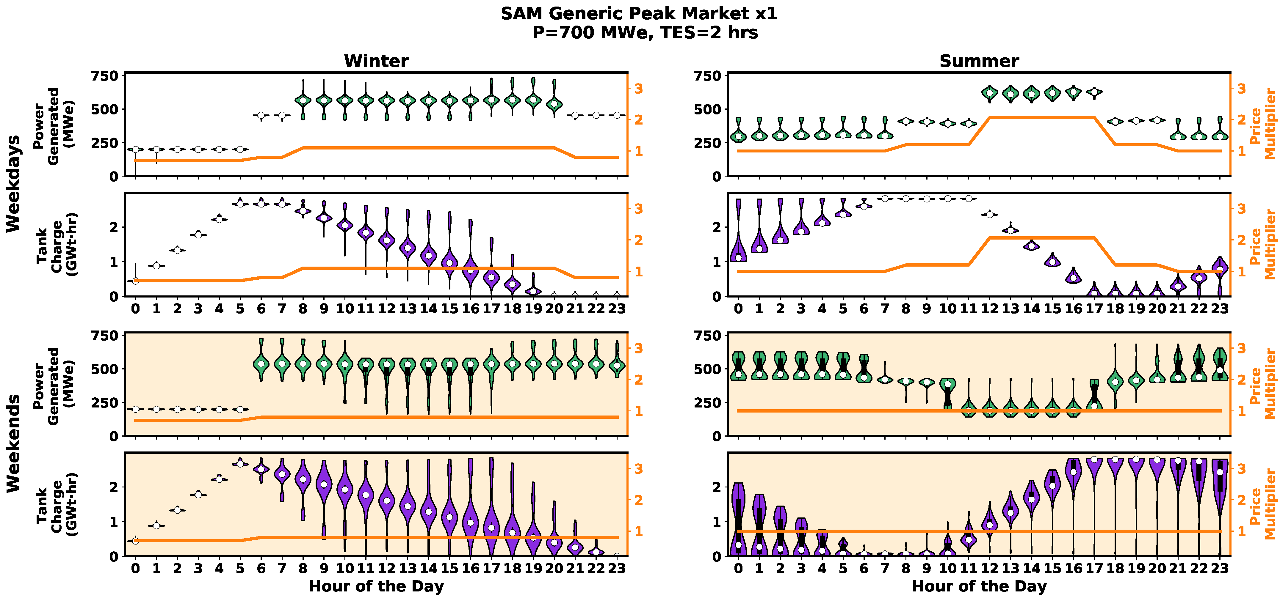
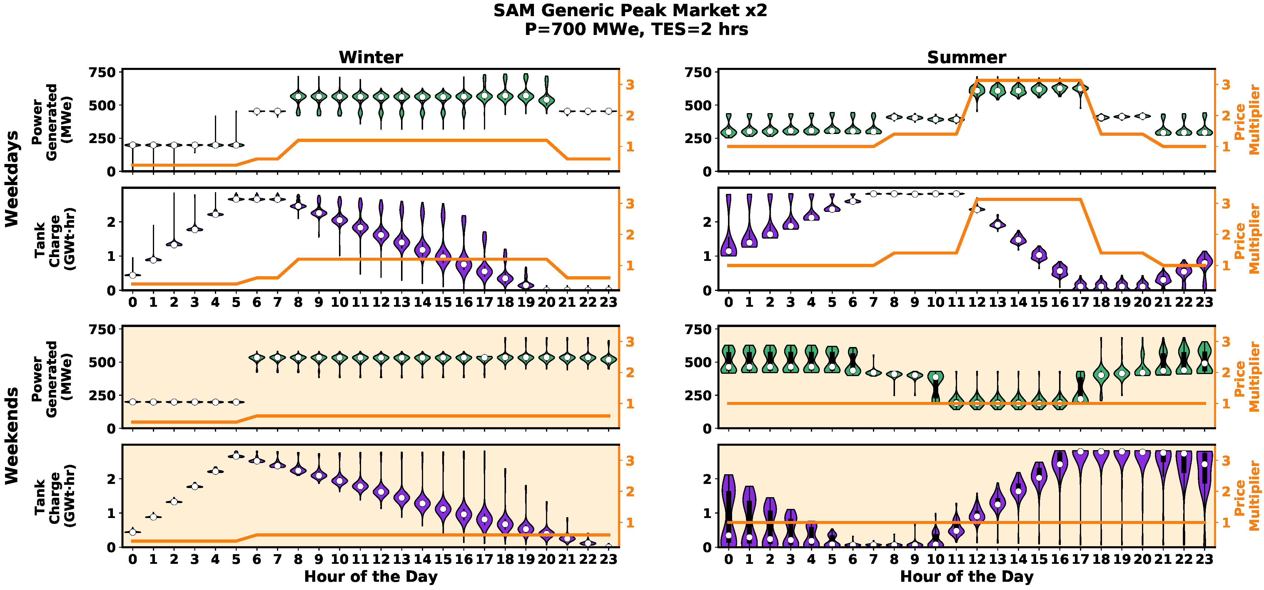
3.1. Load Profiles for Plant with 700 MW_e, 2 h of TES, under SAM Tariff Rates

We highlight operation profiles for some illustrative cases of turbine power output, TES capacity, and market scenarios. Figure 4 shows results for a 700 MW_e turbine design with 2 h of thermal storage operating in the generic peak market from SAM. The hourly generated power output of the power cycle and energy levels of the TES are tallied for a full simulated year. We then create a violin plot for both metrics, demonstrating the distribution in values for each hour of the day throughout the year. We further categorize the hourly distributions according to the seasonal and daily variations in SAM tariff levels shown in Figure 2: subplots distinguish between winter versus summer tariffs in the columns; each column is then subdivided between weekday versus weekend tariffs. Together, these subplots reveal the distributions in daily operating levels given pre-defined seasonal and weekly market variability.

Some routine behavior of the plant is evident from Figure 4. Between midnight and 5 a.m. during winter weekdays, power generation is kept at a low level while energy prices are relatively low (i.e., the price multiplier is below 1). A greater portion of nuclear thermal power is instead routed to storage as shown by the increasing tank charge level during those same hours. Power generation during winter weekdays then increases from the low morning levels with ∼450 MW_e contributions from the LFR and the rest coming from thermal storage. Tank energy levels decrease steadily between 8 a.m. and 8 p.m. as excess energy is dispatched to the power cycle; day-by-day variability in the targeted dispatch is based on anticipated outside dry temperatures and efficiency losses. Tank levels are mostly depleted by 8 p.m., after which the cycle runs with just the nuclear thermal contribution until midnight where the process is repeated.

Winter weekend behavior differs from weekday behavior due to the much smaller ramp in tariff rates in the early morning hours. Prices increase only once during winter weekend days as opposed to twice during weekdays for the same amount of hours. While on weekdays the plant often chooses to wait until the second, higher price ramp at 8AM before dispatching energy from storage, on weekends the plant dispatches starting at the singular price increase at 6AM. The plant then dispatches excess energy for longer as a response to the static market signal.

Summer weekday behavior for the plant design in Figure 4 mimics the winter weekdays behavior with some adjustments due to seasonal differences in the proposed SAM market profile. The highest price peak for summer weekdays is larger but narrower in time; the tanks, with their limited capacity, choose to dispatch their inventory more quickly during the tallest peak. This is demonstrated by a steeper slope in the tank energy decrease between 11am and 5 p.m. Thermal storage charging also commences earlier than during the winter, starting in the late hours of the night rather than at midnight. The earlier start is met by a slower charge time—a higher portion of the hourly nuclear thermal output is instead routed directly to the power cycle to operate at slightly higher power levels than winter weekdays.

Summer weekend behavior contrasts with the other three seasonal scenarios as the tanks generally charge during the daytime as opposed to the early morning hours. Tariff rates are static throughout the entire day; rather than follow market signals, tank storage levels instead anticipate hot midday temperatures that lower efficiency and therefore total power generation. Energy therefore dispatches at night to avoid daytime losses. Tank levels and energy production from midnight to 6 a.m. exhibit bi-modal behavior; depending on when the weather is more advantageous, the system will choose whether to operate with full or partial contribution from thermal storage.

To better understand the role of price ramping on the techno-economic performance of the plant, we created additional modified market profiles based on the original SAM generic peak rates. From the base tariff schedule, all differences from unity are amplified by a factor of two. This results in price multipliers with more exaggerated peaks and troughs and therefore more dramatic price ramping. Figure 5 shows a distribution of hourly behavior for the same design, with 700 MW_e and 2 h of thermal storage, but under the SAM market with exaggerated ramps. Across both winter and summer weekdays, the behavior is largely unchanged from the base tariff schedule. Winter weekend hourly distribution of both energy produced and energy dispatched have much less spread. The more uniform operating levels throughout the year imply less sensitivity to variable dry temperatures. The benefits of operating under more volatile pricing markets become more evident from the economics of the plant and are discussed in Section 3.4.

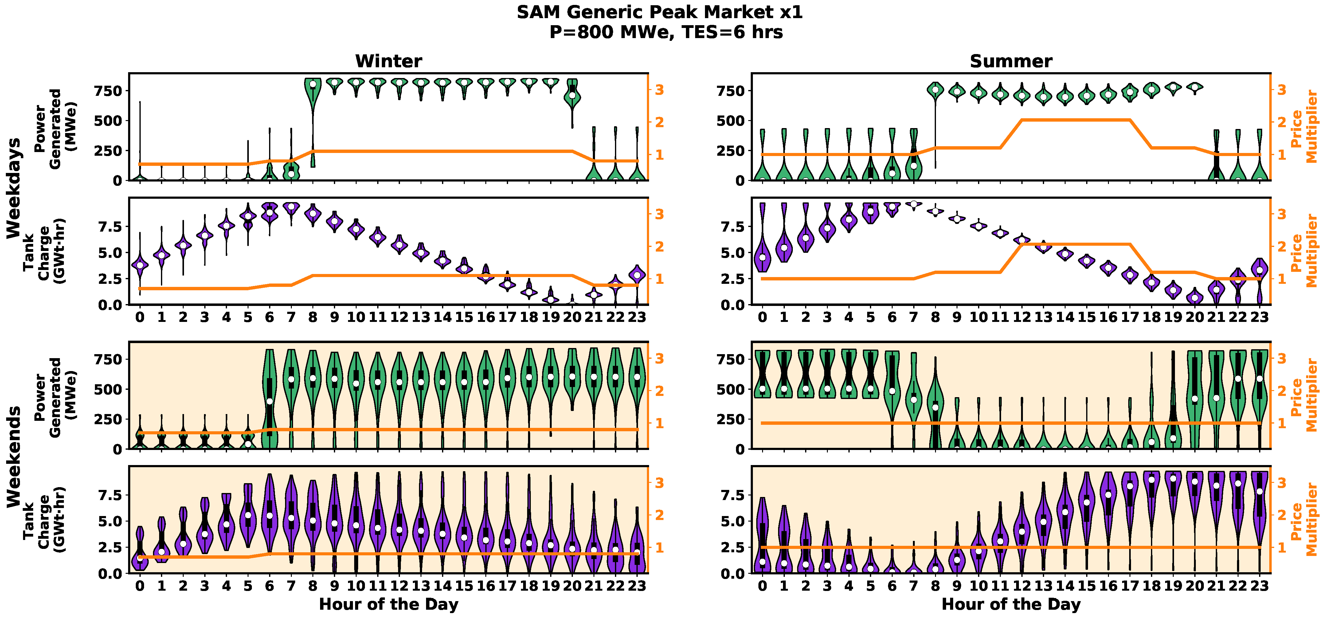
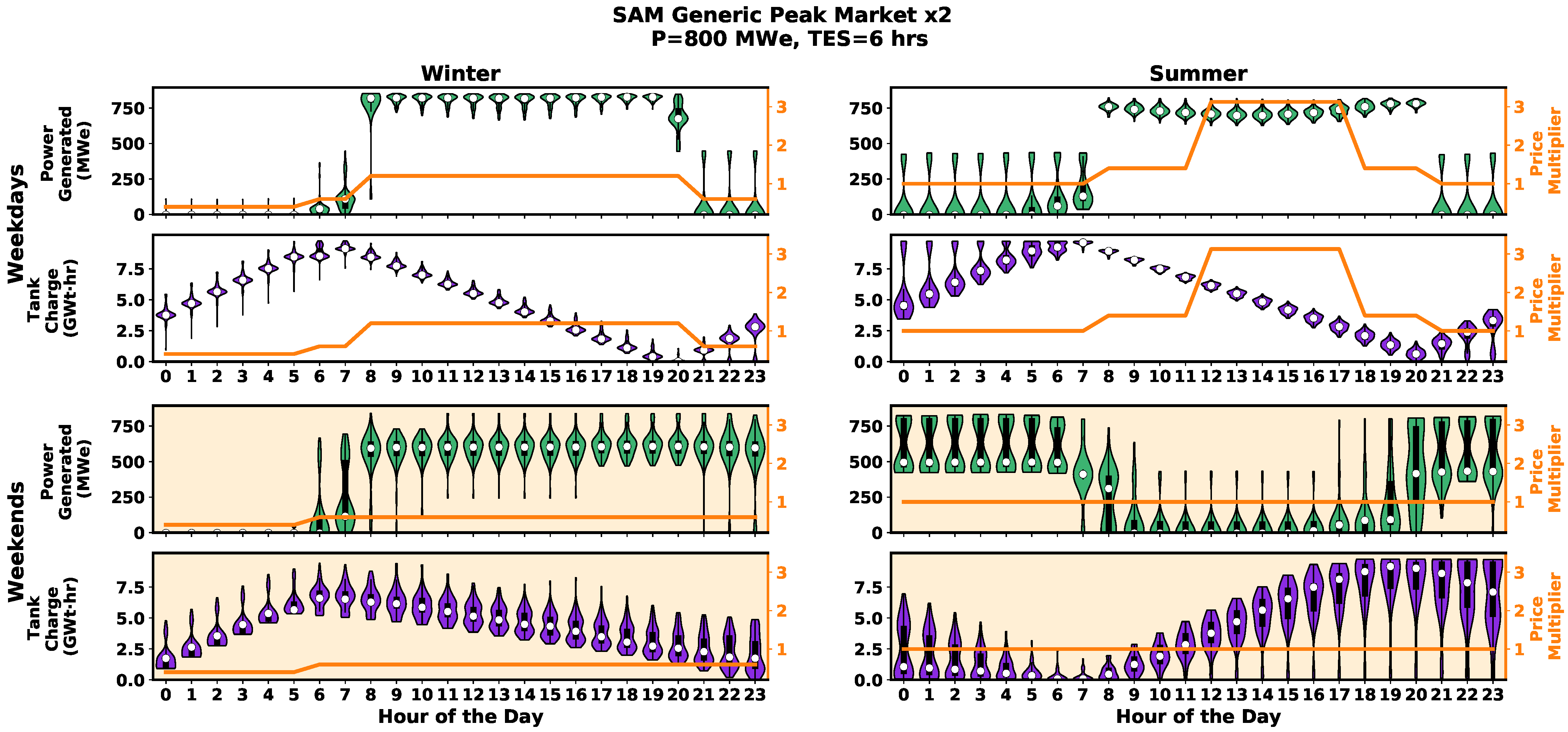
3.2. Load Profiles for Plant wtih 800 MW_e, 6 h of TES, under SAM Tariff Rates

We next highlight operation profiles for a case with larger thermal storage capacity. Figure 6 shows hourly distributions of power generation and energy storage levels for an 800 MW_e turbine with 6 h of thermal storage. With the extra storage capacity, power generation is more likely to shut-off during low pricing periods in order to focus more generation during higher pricing periods. Storage is particularly prioritized in the winter weekday mornings between 12 a.m. and 8 a.m. in anticipation of high daytime prices. Additional costs are incurred from power cycle shutdown and startup operations but are not prohibitive due to high daytime revenues. Generally, any pricing periods with multipliers greater than one are met with high power generation from both nuclear and thermal storage contributions regardless of season. This is best illustrated by the contrast between the winter and summer weekday distributions of this design compared with those of the smaller storage capacity design in Figure 4. In the smaller storage capacity case, the power generation scales more closely with each price multiplier increase due to the reduced energy capacity available for dispatch in the molten salt tanks, accentuated by the 5 h lag between complete tank fill-up and discharge ahead of the summer weekday noon price hike. In the 800 MW_e design, with 6 h of thermal storage, the tanks can contribute more energy for longer.

Figure 7 shows operation profiles for the same 800 MW_e and 6 h of storage plant but under the modified peak market from SAM with twice-amplified peaks and troughs. The plant behavior does not change dramatically except for some slightly faster ramping in power generation immediately preceding weekday daytime price increases. Weekend tank level distributions are also narrower similar to Figure 5.

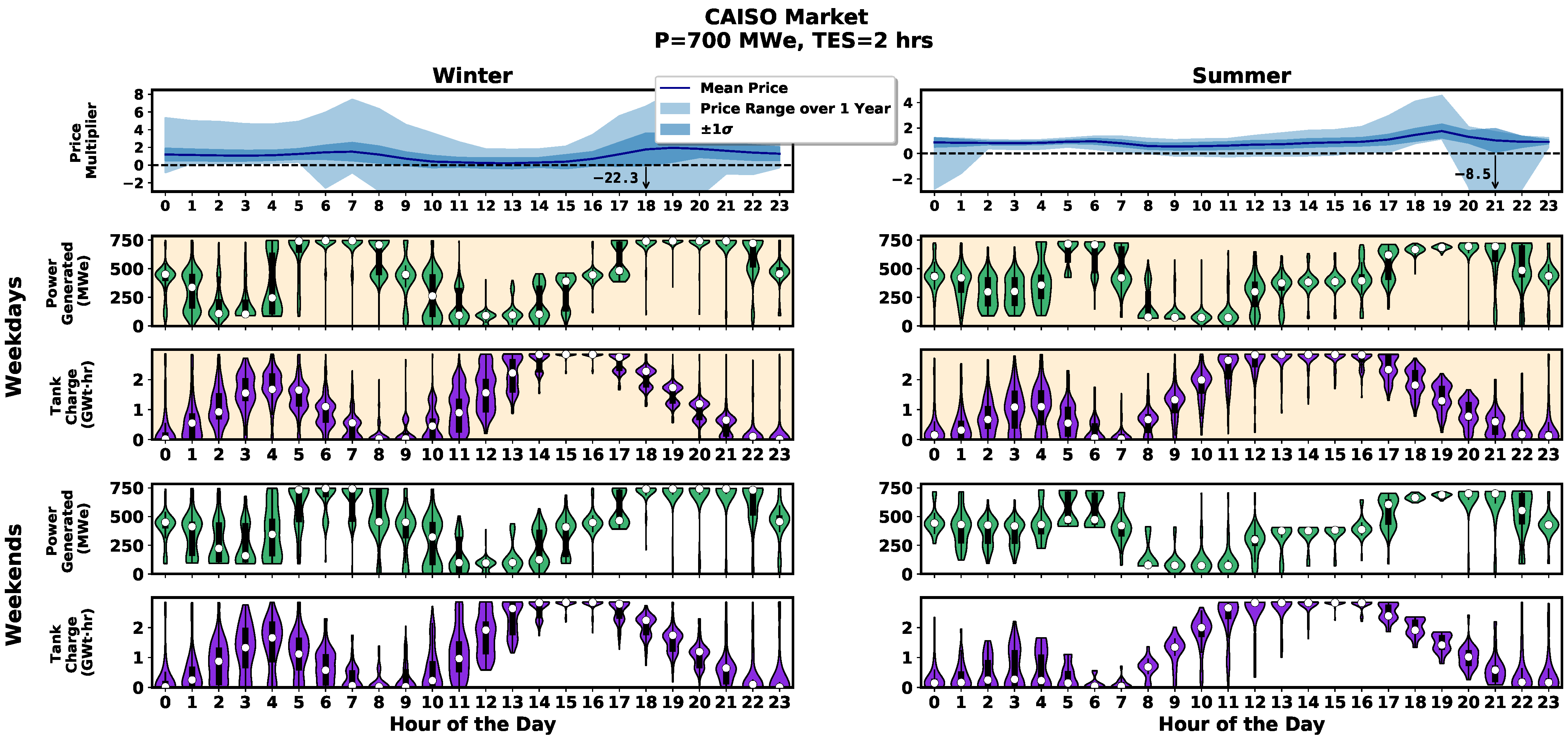
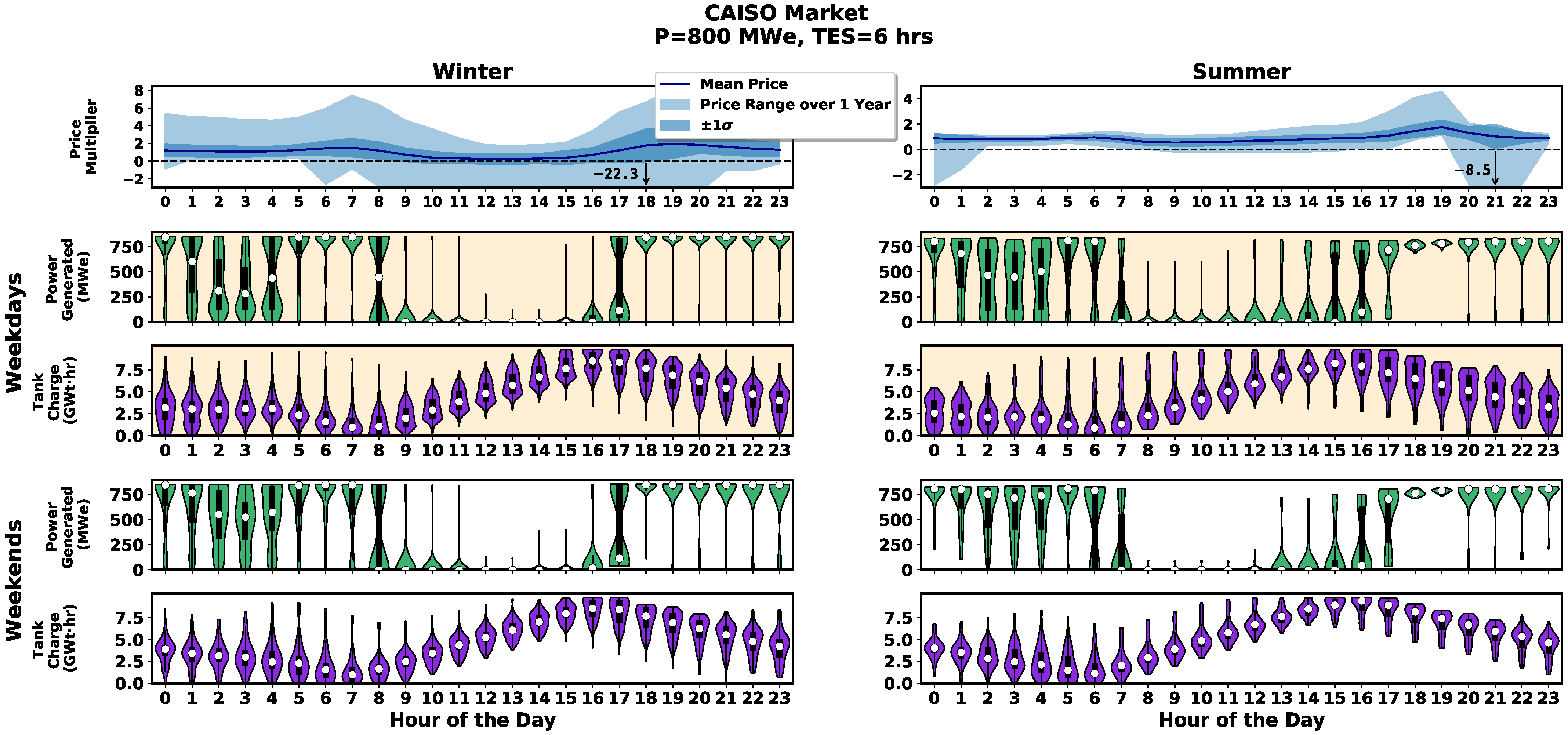
3.3. Load Profiles for Both Plant Cases under CAISO Market Conditions

We also simulate the performance of the coupled nuclear and TES system under CAISO tariff rates from Figure 2. Simulated plant performance here would be more indicative of expected performance in a VRE-saturated market like California. Figure 8 shows hourly distributions for a 700 MW_e turbine with 2 h of storage under CAISO market conditions. Power generation and storage charge level for both winter and summer have much more variable hourly distributions due to the increased volatility in market prices. However, it is evident that two charging periods occur on most days regardless of season: in the early morning and during midday hours. These charging periods precede higher peaks in energy pricing during morning and late afternoon hours. The charging periods also sometimes coincide with negative energy prices, giving the plant an alternative use for the nuclear thermal energy other than producing electricity at a loss. Winter and summer profiles differ mostly by the temporal location of the price peaks. Storage charging in the winter seems to start 1–2 h later than summer charging, likely due to a later sunrise which denotes the daily introduction of solar renewable energy into the grid and a subsequent lowering of prices. There are no notable differences between weekend and weekday behavior for the plant.

An increase in storage capacity is simulated again with the 800 MW_e and 6 storage hours under the same CAISO market scenario. Figure 9 shows more uniform trends compared to the lower capacity case in Figure 8. With higher storage capacity, the optimized charge level profile follows a sinusoid with a single daily peak: rather than dispatch energy for both the morning and evening price peaks, it prioritizes the evening price peak with more lucrative prices. Midday generation is more likely to shut down during midday prices, regardless of season, to use all of the nuclear thermal availability for storage.

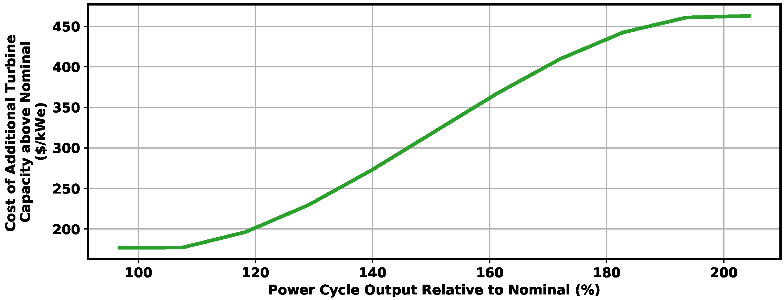
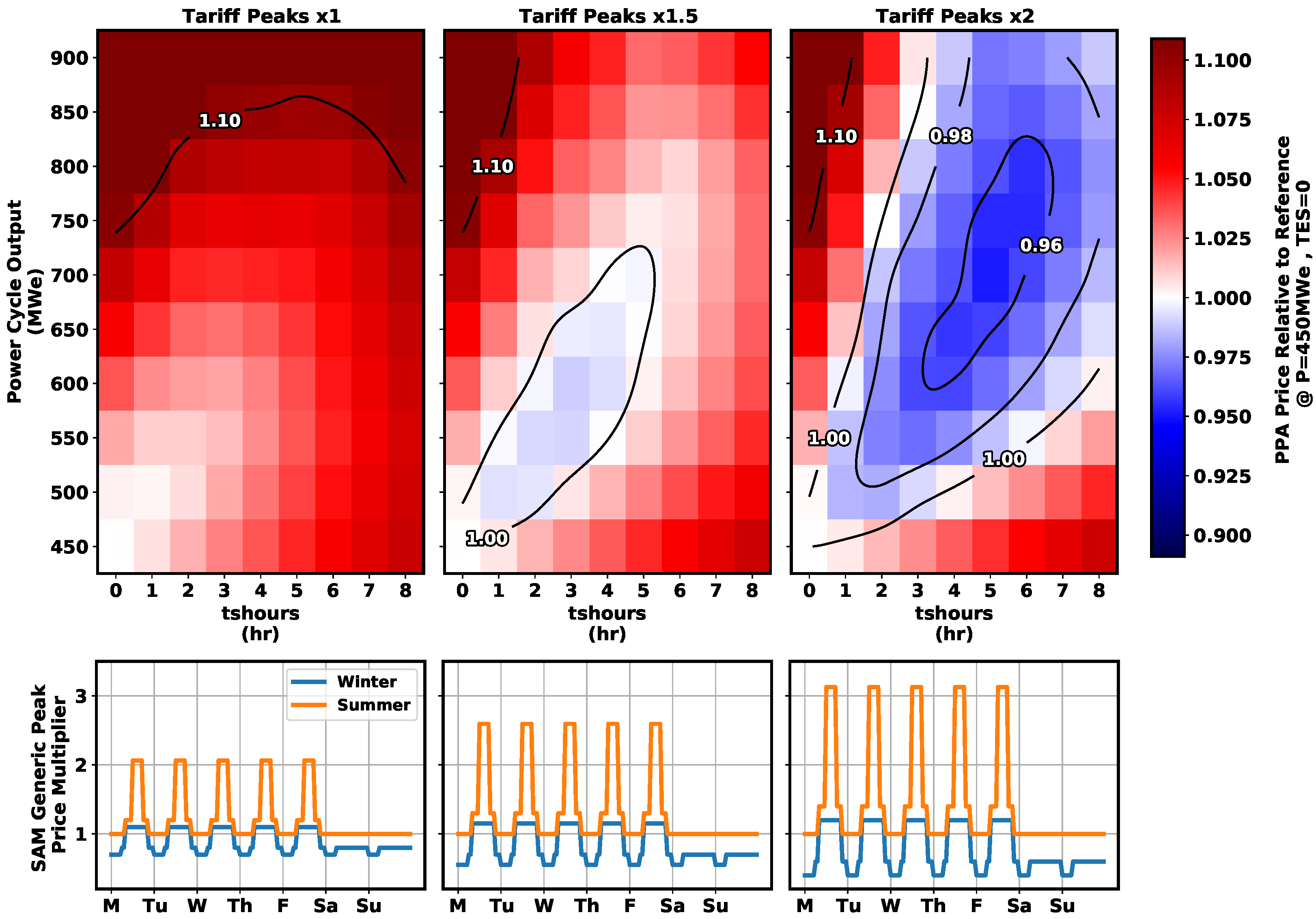
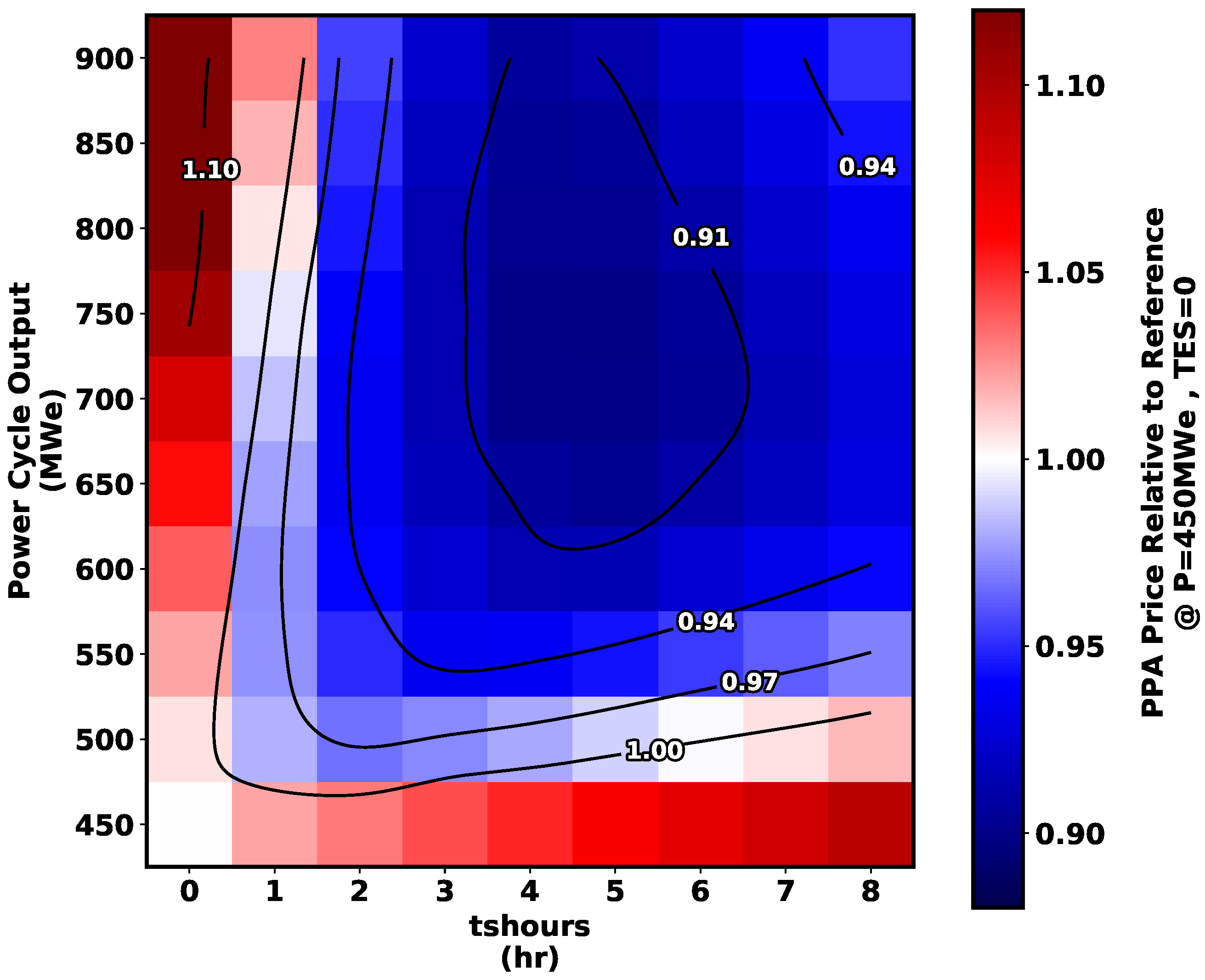
3.4. Plant Sizing Trade Studies

The variation in power generation and operation profiles between low and high capacity storage designs prompts the question of optimal tank capacity and the corresponding over-sizing of the power cycle turbine. The answer would seem to depend on the volatility of the market based on the previous load profiles. One way to imitate a scaling of volatility is by using the generic SAM peaking market and gradually exaggerating the values above and below unity, as conducted in the previous section. We have generated several price multiplier curves in the bottom row of Figure 10 with amplification factors ranging between 1 and 2. For each of these exaggerated peak markets, we conducted a parameter sweep over the nominal power cycle output in MW_e and hours of thermal storage, generating a full year simulation for each. Results of the parameter sweep over each market scenario are plotted as a heat map in their corresponding column within Figure 10. The color value of each 2-D plot represents a relative PPA price: the PPA price for each element is normalized by the PPA price of the reference design (having no storage and turbine matching the nuclear thermal output). Relative PPA prices lower than 1 represent design points more desirable than the reference case and therefore a subset of the parameter space where adding thermal storage to the nuclear plant is economically advantageous.

Starting with the leftmost column of Figure 10, under the standard SAM generic peak market, no amount of thermal storage reduces the PPA price below the nominal design point. The pricing signals are not high enough to offset any additional costs incurred by building and operating the thermal tanks. Adding any storage to the nominal 450 MW_e turbine strictly increases the PPA price as the power plant can never operate above nominal output and there is hence no price advantage to charging the TES. Separately, sizing up the power plant past the reference design point naturally worsens economic performance with increased turbine costs and no extra energy to sell from storage. Adding thermal storage to plants with output higher than 450 MW_e does improve the performance relative to the respective case with no thermal storage; however, the improvements in the generic peak market are never better than the reference and have diminishing returns when adding more than 5 h of storage.

The second column of Figure 10 shows a slightly more exaggerated market profile—where peaks and troughs about the 1 value are amplified by 50%—than the leftmost plot. Relative PPA prices are again calculated relative to the reference design PPA price but this time under the new market conditions. We overlay a contour denoting the region in the parameter space where relative PPA values fall below 1—that is, a region forms where adding thermal storage to the power plant and slightly over-sizing the turbine output improves the performance relative to the reference, no-TES case. Improvements are marginal within this market at approximately 1% but they suggest a trend.

The trend is confirmed by the rightmost plot where tariff rate peaks are amplified by a factor of 2. The region of improved economic performance has expanded to now span 8 h of thermal storage and include solutions with up to 900 MW_e, a turbine oversized by 200%. Though many solutions exist that perform better than the reference, the optimal design point within this market for PPA price is at 700 MW_e and 5 h of available thermal storage with 5% improvements in PPA price. Final PPA prices for all markets are shown in

Table 4. Optimal plant designs and corresponding PPA prices per market.

Market Scenario	Optimal Turbine Size (MWe)	Optimal TES Size (h)	Optimal PPA Price (¢/kWe·h)
SAM Generic Peak ×1.0	450	0	6.54
SAM Generic Peak ×1.5	600	3	6.49
SAM Generic Peak ×2.0	700	5	6.26
CAISO	750	5	5.63

. We see that for a given turbine size above the nominal there exists an optimal TES size able to store enough energy to maximize turbine output over periods of peak pricing.

Performances using the market signal amplification tactic show the effects of increased price ramping on the final PPA price. We additionally quantify the performance of the combined LFR and TES plant using the CAISO tariffs from Figure 2, taken from real energy prices and normalized to not artificially inflate revenue. Figure 11 show a similar heatmap of relative PPA prices to the reference 450 MW_e and 0 h of thermal storage design evaluated using CAISO tariff rates. The region of improved design points expands much further than even the twice amplified peaks in Figure 10; the improvements are greater in value as well. Only under certain cases does the plant perform worse than the reference design: heavily over-sized power outputs paired with low amounts of thermal storage and slightly over-sized power outputs paired with large amounts of thermal storage. In each case, any additional revenue from selling stored energy—even when dispatched optimally—does not offset costs incurred from oversizing the respective subsystem. The optimal design point for system performance in the CAISO market is similar to the twice amplified SAM generic peak market: a 750 MW_e with 5 h of thermal storage results in 10% improvements in PPA price.

3.5. Sensitivity Analysis on Thermal Storage Costs

The LFR performance when coupled with TES was analyzed in the previous sections using static costs with the exception of the turbine cost per unit power, which scaled as a cubic function of the rated nominal turbine rating shown in Figure 3. Among the other parameters to which our simulations might be sensitive to, the thermal storage cost would pose the highest second-order effect as it pertains to one of the main subsystems of the plant. From Table 1, we estimate the cost of the thermal storage at $29.8 per kWt·h based on similar costs of molten salt tanks paired with CSP systems. To determine whether thermal storage costs were indeed a higher-order effect on the PPA price, we conducted a sensitivity analysis on the previous simulations by varying the TES cost between 20–60 $/kWt·h for selected designs. Results are shown in Figure 12. Each row within the figure represents a different market scenario: SAM generic peak market, the same market with twice-amplified peaks, and the normalized CAISO market. For the three markets, each column represents a selected turbine output. Each individual plot then shows PPA price relative to that of the reference plant design under the respective market as a function of thermal storage hours. Multiple curves in each plot represent performance under varying TES cost (with the reference cost shown in black). The optimal power cycle output and storage amount for each market scenario are highlighted and marked with dotted vertical lines; the relative PPA price of 1 is also marked with a horizontal line for reference.

Together, the plots in Figure 12 show little deviation from previous trends when altering TES costs. The PPA price of the optimal design point naturally worsens and improves as TES costs increase and decrease, respectively. For the SAM generic peak market, performance of a 500 MW_e turbine with 2 h of storage comes close to rivaling the reference design point when lowering the TES cost to $20 per kWt·h but ultimately does not cross the margins. The more volatile markets in the second and third row exhibit the same trend. Here, lower TES costs improve the relative PPA price past the reference. Increasing the TES cost reveals price points where thermal storage would no longer be advantageous. For the CAISO markets in the third row, all shown combinations outperform the plant with no storage except for the highest estimated cost with 7 h of storage.

As mentioned previously, we do not model a thermodynamic efficiency penalty when integrating the TES with the nuclear reactor. Efficiency penalties for the TES would be highly dependent on the configuration; omitting them allows the model and subsequent results to remain more generalizable but might result in a slight overestimation of performance with the TES. For our direct configuration for TES charging shown in Figure 1, we would expect a reduction in efficiency for values of tshours greater than 0 due to inclusion of an additional loop between the primary and the power conversion cycle with associated temperature losses. If the efficiency penalty were to drop by 1–2 percentage points this would correspond to roughly 2–5% reduction in the electrical power produced. Ultimately, this would introduce a step shift in PPA price for non-zero values of TES storage.

Table 5. Sensitivity of optimal design point to efficiency penalty incurred by implementing TES. PPA price improvements are calculated relative to reference design performance in the respective market.

Market Scenario	Optimal Turbine Size (MWe)				Optimal TES Size (h)				PPA Price Improvement (%, Relative to Reference)
Performance Penalties:	0%	1%	2.5%	5%	0%	1%	2.5%	5%	0%	1%	2.5%	5%
SAM Generic Peak × 1.0	450	←1	←	←	0	←	←	←	0	←	←	←
SAM Generic Peak × 1.5	600	←	450	←	3	←	0	←	1.05	0.06	0	←
SAM Generic Peak × 2.0	700	←	←	←	5	←	←	←	4.88	3.93	2.50	0.13
CAISO	750	←	←	←	5	←	←	←	10.06	9.16	7.81	5.57

¹ A left arrow (←) denotes a table element equivalent to the value of its left-adjacent column.

shows the sensitivity of the optimal design point when a performance penalty is imposed on the final PPA price (only for designs with storage). The optimal design for the SAM tariff rates is only affected by the TES efficiency penalty in markets where the tariff peak amplification factor is below two: adding performance penalties changes the optimal design to one without TES. The design point does not change for the twice-amplified SAM and the CAISO tariff schedules when imposing the additional TES efficiency penalty. However, improvements on PPA price from the additional TES in these markets are reduced with increasing performance penalties. They nevertheless still perform better than the reference no-storage design.

For the indirect TES case not modeled here, described in Section 2.1, there would not be a universal efficiency penalty for non-zero amounts of storage. However, we would expect round-trip efficiency penalties on energy that is stored prior to dispatch that might move the optimal point closer to the origin of the plots in Figure 10 and Figure 11. The indirect TES model will be a subject of future studies.

4. Discussion

The volatility of energy market pricing as a consequence of daily and hourly VRE availability incentivizes more flexible dispatchability for nuclear power plants. We have shown, for a medium-sized NPP rated at 950 MWt, that coupling molten salt thermal storage improves economic performance only when participating in volatile markets where ramping is necessary and therefore rewarded with higher prices. With a novel software architecture that combines the robust engineering model of SAM and a mixed-integer linear program for dispatch optimization, we now can simulate a coupled NPP and thermal storage plant under varying market and weather conditions. Technical operations of our LFR and TES design, modeled after the Westinghouse LFR concept, have been shown to prioritize thermal power from the nuclear component according to price increases. Thermal power is typically stored in the molten salt tanks ahead of pricing peaks; charging periods are also used advantageously during negative pricing periods in the CAISO market simulations and ahead of particularly hot dry temperature periods when pricing curves are flat and offer no incentive. Dispatch of stored energy is most effective during high pricing periods, offering increased revenue to offset any low powered periods of power cycle operation or even power cycle shutdowns occurring during storage charging periods.

Our results assume perfect forecasting of both pricing and weather data over 48 h periods which might not be entirely realistic; future work in adapting forecasting models to the optimal dispatch strategy would help create more accurate depictions of system performance. Siting and participation in grid-stabilizing ancillary service markets is also of interest for future study. A companion model for the indirect TES configuration is currently being developed for investigation.

5. Conclusions

The economic performance of the system was shown to improve as a function of market price volatility. With the single-peak SAM market and subsequent peak magnifications, we showed that increased price ramping creates and amplifies a region of improved performance in the turbine oversizing versus thermal storage parameter space. Designs within the region outperform a design with no thermal storage and turbine electric output that matches the assumed NPP thermal input. The outperforming region moves towards higher thermal storage and more oversized turbine designs as the volatility is increased. With the assumed costs in this simulation, PPA price reaches a minimum under the CAISO market simulations with up to a 10% improvement in performance relative to the reference design. A sensitivity analysis of TES cost confirms that when operating in the CAISO market, the NPP-TES design outperforms the reference design for TES costs up to double the assumed value (except for designs with large amounts of storage, close to 7 h). Despite additional costs incurred, it is still economically advantageous to both add thermal storage capabilities and correspondingly oversize the turbine electric output for plants performing in volatile energy markets saturated by variable renewable energy.

References

1. Denholm, P.; O’Connell, M.; Brinkman, G.; Jorgenson, J. Overgeneration from Solar Energy in California. A Field Guide to the Duck Chart; No. NREL/TP-6A20-65023; National Renewable Energy Lab.: Golden, CO, USA, 2015; Volume 1. [CrossRef] [Green Version]
2. Stansbury, C. Westinghouse Modular Heat Storage: A Flexible Approach to Next Generation Grid Needs. Heat Storage for Gen IV Reactors for Variable Electricity from Base-Load Reactors; Idaho National Laboratory: Idaho Falls, ID, USA, 2019.
3. Forsberg, C.; Sabharwall, P.; Sowder, A. Separating Nuclear Reactors from the Power Block with Heat Storage: A New Power Plant Design Paradigm; Idaho National Laboratory: Idaho Falls, ID, USA, 2020.
4. Forsberg, C.; Sabharwall, P.; Gougar, H.D. Heat Storage Coupled to Generation IV Reactors for Variable Electricity from Base-load Reactors: Workshop Proceedings: Changing Markets, Technology, Nuclear-Renewables Integration and Synergisms with Solar Thermal Power Systems; Idaho National Laboratory: Idaho Falls, ID, USA, 2019.
5. Wald, M. With Natrium, Nuclear Can Pair Perfectly with Energy Storage and Renewables. NEI. 2020. Available online: https://www.nei.org/news/2020/natrium-nuclear-pairs-renewables-energy-storage (accessed on 20 March 2022).
6. USNC. USNC Micro Modular Reactor (MMR™ Block 1) Technical Information; USNC: Seattle, WA, USA, 2021. [Google Scholar]
7. Oh, S.; Lee, J.I. Performance Analysis of Thermal Energy Storage System For Nuclear Power Plant Application; Korean Nuclear Society: Seoul, Korea, 2021. [Google Scholar]
8. Alameri, S.A.; King, J.C. A Coupled Nuclear Reactor Thermal Energy Storage System for Enhanced Load Following Operation. In 2013 International Nuclear Atlantic Conference; ABEN: Recife, PE, Brazil, 2013; pp. 173–182. [Google Scholar]
9. Romanos, P.; Al Kindi, A.A.; Pantaleo, A.M.; Markides, C.N. Flexible nuclear plants with thermal energy storage and secondary power cycles: Virtual power plant integration in a UK energy system case study. e-Prime-Adv. Electr. Eng. Electron. Energy 2022, 2, 100027. [Google Scholar] [CrossRef]
10. Stansbury, C.; Smith, M.; Ferroni, P.; Harkness, A.; Franceschini, F. Westinghouse Lead Fast Reactor Development: Safety and Economics Can Coexist. In Proceedings of the 2018 International Congress on Advances in Nuclear Power Plants, Charlotte, NC, USA, 8–11 April 2018. [Google Scholar]
11. Westinghouse Electric Company, U.S.A. Westinghouse Electric Company, U.S.A. Westinghouse Lead Fast Reactor. In Advances in Small Modular Reactor Technology Developments; IAEA Advanced Reactors Information System: Vienna, Austria, 2020; pp. 233–236. [Google Scholar]
12. Blair, N.; Diorio, N.; Freeman, J.; Gilman, P.; Janzou, S.; Neises, T.; Wagner, M. System Advisor Model (SAM) General Description (Version 2017.9.5); National Renewable Energy Laboratory Technical Report; National Renewable Energy Lab.: Golden, CO, USA, 2018.
13. Smith, C.F.; Halsey, W.G.; Brown, N.W.; Sienicki, J.J.; Moisseytsev, A.; Wade, D.C. SSTAR: The US lead-cooled fast reactor (LFR). J. Nucl. Mater. 2008, 376, 255–259. [Google Scholar] [CrossRef] [Green Version]
14. Smirnov, V.; Orlov, V.; Mourogov, A.; Lecarpentier, D.; Ivanova, T. The lead cooled fast reactor benchmark BREST-300: Analysis with sensitivity method. In Nuclear Data Needs For Generation IV Nuclear Energy Systems; World Scientific: Singapore, 2006; pp. 173–182. [Google Scholar]
15. Abderrahim, H.A.; Bruyn, D.D.; Dierckx, M.; Fernandez, R.; Popescu, L.; Schyns, M.; Stankovskiy, A.; Eynde, I.; Gert, V.d.; Vandeplassche, D. MYRRHA accelerator driven system programme: Recent progress and perspectives. News High. Educ. Inst. Nucl. Energy 2019, 2, 29–42. [Google Scholar]
16. Smith, C.; Cinotti, L. Lead-cooled fast reactor. In Handbook of Generation IV Nuclear Reactors; Pioro, I.L., Ed.; Woodhead Publishing Series in Energy; Woodhead Publishing: Sawston, UK, 2016; Chapter 6; pp. 119–155. [Google Scholar] [CrossRef]
17. Alemberti, A.; Smirnov, V.; Smith, C.F.; Takahashi, M. Overview of lead-cooled fast reactor activities. Prog. Nucl. Energy 2014, 77, 300–307. [Google Scholar] [CrossRef]
18. Alemberti, A. Lead cooled fast reactors. In Reference Module in Earth Systems and Environmental Sciences; Elsevier: Amsterdam, The Netherlands, 2020. [Google Scholar] [CrossRef]
19. Delameter, W.; Bergan, N. Review of the Molten Salt Electric Experiment; Report SAND86-8249; Sandia National Laboratories: Albuquerque, NM, USA, 1986.
20. White, B.T.; Wagner, M.J.; Neises, T.; Stansbury, C.; Lindley, B. Modeling of Combined Lead Fast Reactor and Concentrating Solar Power Supercritical Carbon Dioxide Cycles to Demonstrate Feasibility, Efficiency Gains, and Cost Reductions. Sustainability 2021, 13, 12428. [Google Scholar] [CrossRef]
21. Hamilton, W.T.; Newman, A.M.; Wagner, M.J.; Braun, R.J. Off-design performance of molten salt-driven Rankine cycles and its impact on the optimal dispatch of concentrating solar power systems. Energy Convers. Manag. 2020, 220, 113025. [Google Scholar] [CrossRef]
22. F-Chart. Engineering Equation Solver. 2022. Available online: https://fchartsoftware.com/ees/ (accessed on 20 March 2022).
23. Wagner, M.J.; Newman, A.M.; Hamilton, W.T.; Braun, R.J. Optimized dispatch in a first-principles concentrating solar power production model. Appl. Energy 2017, 203, 959–971. [Google Scholar] [CrossRef]
24. Kahvecioglu, G.; Morton, D.; Wagner, M. Dispatch Optimization of a Concentrating Solar Power System Under Uncertain Solar Irradiance and Energy Prices. Appl. Energy, 2022; Submitted, In Review. [Google Scholar]
25. CAISO. Open Access Same-Time Information System. 2022. Available online: http://oasis.caiso.com/mrioasis/logon.do (accessed on 30 August 2021).
26. Kumar, N.; Besuner, P.; Lefton, S.; Agan, D.; Janzou, S.; Hilleman, D. Power Plant Cycling Costs; Technical Report; National Renewable Energy Laboratory: Golden, CO, USA, 2012.
27. Cox, J.; Hamilton, W.; Newman, A.; Zolan, A.; Wagner, M. Real-time Dispatch Optimization for Concentrating Solar Power with Thermal Energy Storage. Optim. Eng. 2022; in press. [Google Scholar]
28. Bynum, M.L.; Hackebeil, G.A.; Hart, W.E.; Laird, C.D.; Nicholson, B.L.; Siirola, J.D.; Watson, J.P.; Woodruff, D.L. Pyomo—Optimization Modeling in Python, 3rd ed.; Springer Science & Business Media: Berlin/Heidelberg, Germany, 2021; Volume 67. [Google Scholar]
29. Forrest, J.; Vigerske, S.; Ralphs, T.; Santos, H.G.; Hafer, L.; Kristjansson, B.; Jpfasano; EdwinStraver; Lubin, M.; Rlougee; et al. Coin-Or/Cbc: Release Releases/2.10.3 2020. Available online: https://zenodo.org/record/3246628#.YoG-DlRBxPY (accessed on 26 October 2020).
Figure 1. Schematic of LFR-molten salt flow loop. LFR heats (via secondary steam loop) the molten salt that flows from the cold to hot storage tanks. The hot tank can then discharge heat to the power cycle leading up to the steam turbine.
Energies 15 03599 g001
Figure 2. Price multipliers used to simulate different market conditions: (top) generic peak pricing schedule from SAM and (bottom) normalized locational marginal price from CAISO. Some negative pricing outliers for CAISO are not directly shown in the axis but are annotated in the graph.
Energies 15 03599 g002
Figure 3. Cost of additional power conversion capacity above nominal turbine.
Energies 15 03599 g003
Figure 4. Hourly violin plot distributions for a year of simulated electric power and stored energy levels. Computed for a 700 MWe turbine with 2 h of TES under SAM generic peak market prices. Median value for each hour is shown as a white circle and the black vertical rectangle demarcates 25th and 75th percentiles. Distributions are split between winter and summer price schedules as well as weekday and weekend prices; price multipliers are shown on the right axis of each subplot.
Energies 15 03599 g004
Figure 5. Hourly violin plot distributions for a year of simulated electric power and stored energy levels. Computed for a 700 MWe turbine with 2 h of TES under twice-amplified SAM generic peak market prices. Median value for each hour is shown as a white circle and the black vertical rectangle demarcates 25th and 75th percentiles. Distributions are split between winter and summer price schedules as well as weekday and weekend prices; price multipliers are shown on the right axis.
Energies 15 03599 g005
Figure 6. Hourly violin plot distributions for a year of simulated electric power and stored energy levels. Computed for a 800 MWe turbine with 6 h of TES under SAM generic peak market prices. Median value for each hour is shown as a white circle and the black vertical rectangle demarcates 25th and 75th percentiles. Distributions are split between winter and summer price schedules as well as weekday and weekend prices; price multipliers are shown on the right axis of each subplot.
Energies 15 03599 g006
Figure 7. Hourly violin plot distributions for a year of simulated electric power and stored energy levels. Computed for an 800 MWe turbine with 6 h of TES under twice-amplified SAM generic peak market prices. Median value for each hour is shown as a white circle and the black vertical rectangle demarcates 25th and 75th percentiles. Distributions are split between winter and summer price schedules as well as weekday and weekend prices; price multipliers are shown on the right axis.
Energies 15 03599 g007
Figure 8. (Top row) Hourly ranges in normalized CAISO energy price multipliers for a full year. Mean price and standard deviation are shown in a darker shade. (Rows 2–5) Hourly violin plot distributions for a year of simulated electric power and stored energy levels. Computed for a 700 MWe turbine with 2 h of TES under normalized CAISO energy prices. Median value for each hour is shown as a white circle and the black vertical rectangle demarcates 25th and 75th percentiles. Distributions are split between winter and summer price schedules as well as weekday and weekend prices.
Energies 15 03599 g008
Figure 9. (Top row) Hourly ranges in normalized CAISO energy price multipliers for a full year. Mean price and standard deviation are shown in a darker shade. (Rows 2–5) Hourly violin plot distributions for a year of simulated electric power and stored energy levels. Computed for an 800 MWe turbine with 6 h of TES under normalized CAISO energy prices. Median value for each hour is shown as a white circle and the black vertical rectangle demarcates 25th and 75th percentiles. Distributions are split between Winter and Summer price schedules as well as weekday and weekend prices.
Energies 15 03599 g009
Figure 10. Effect of increased price ramping on final PPA price. Each column represents PPA price results for the SAM generic tariff rates with increasing peak-amplification from left to right. Heatmaps show PPA prices relative to the reference design at 450 MWe and 0 h of storage for each market scenario. Contours are generated using interpolated data to highlight key regions: values higher than 1 perform worse than the reference; values lower than 1 perform better. Values higher than 1.1 are not shown for clarity. Corresponding tariff rates shown in bottom row for each column.
Energies 15 03599 g010
Figure 11. Performance of LFR and TES plant in a simulated CAISO market using normalized price multipliers. Heatmap plots PPA price values relative to the reference design at 450 MWe and 0 h of thermal storage. Contours are generated using interpolated data to highlight key regions: values higher than 1 perform worse than the reference; values lower than 1 perform better. Values higher than 1.1 are not shown for clarity.
Energies 15 03599 g011
Figure 12. Sensitivity of PPA price to TES cost. Plots are arranged by different market scenarios in the rows and power cycle outputs in the columns. Individual plots show PPA price relative to the reference design performance (marked as a horizontal line at a value of 1.0) as a function of thermal storage hours. Multiple lines are shown per plot for varying TES cost. Optimal design points are highlighted for each market scenario: the optimal electrical output column is highlighted by face color and the corresponding storage size is marked by a vertical line.
Energies 15 03599 g012