
OC6 Phase Ia: CFD Simulations of the Free-Decay Motion of the DeepCwind Semisubmersible

 , , , , , , , , , , ,
Abstract
:1. Introduction
- (1)
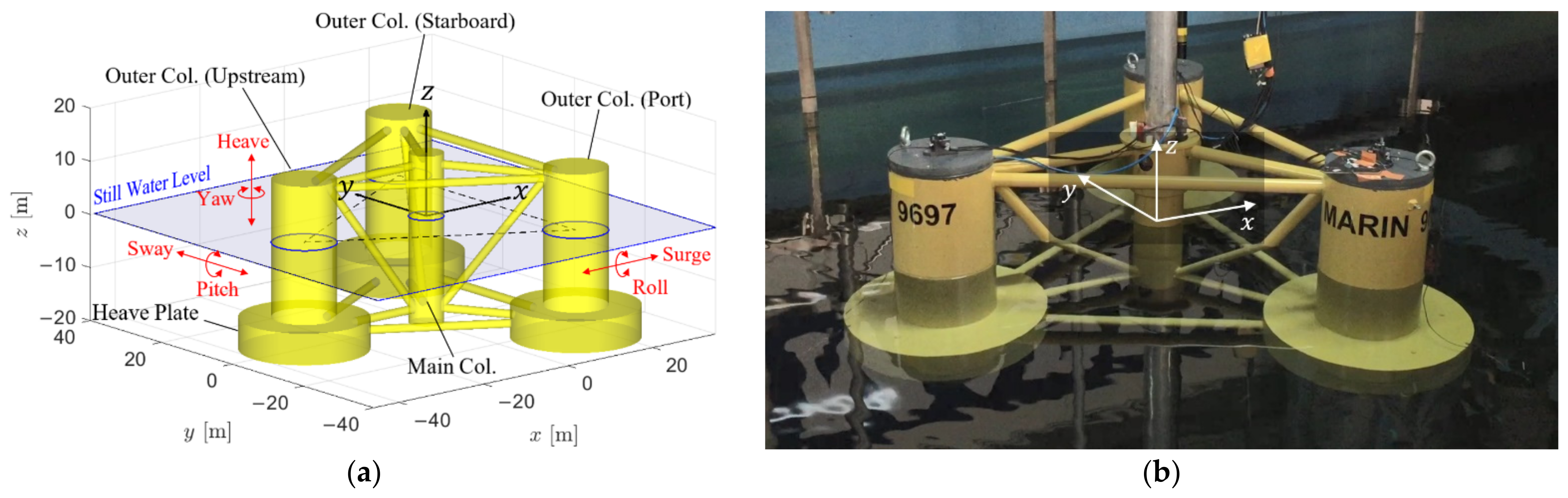
- The CFD simulations are validated against the measurements from a new experimental campaign from OC6 Phase Ia [9,10] specifically designed to minimize uncertainties in the experiment and to focus on the hydrodynamic problem better. The new campaign used a simplified linear taut-spring mooring system instead of the catenary mooring system in the prior OC5 project [7,8], which was frequently identified as one of the major obstacles preventing a successful validation [15,19,20]. The linear-spring mooring setup was developed to provide approximately the correct natural periods of floater motion while greatly reducing the uncertainties and difficulties associated with the numerical modeling of the mooring lines. The wind turbine and tower in the OC5 experiment were also replaced with a rigid bar and a block mass with similar inertial properties to minimize the effects of wind loading and tower flexibility. Compared to the OC5 experiment, the new design of the OC6 experimental campaign minimizes potential physical differences between the experimental and the numerical CFD setups to facilitate validation.
- (2)
- All CFD simulations in the present investigation have a full 6DoF floater motion. Effort was made to replicate the motion of the floater in the experiment in all directions, including the ones not directly relevant to the estimation of damping coefficients.
- (3)
- The uncertainty analysis for the numerical solutions is directly based on the linear and quadratic damping coefficients and the equivalent linear damping ratios estimated from the free-decay motion of the structure. This is different from prior investigations, which typically examined the uncertainty of more basic quantities, such as the maxima in the displacement of the structure. While these basic quantities are less affected by postprocessing and thus are better-suited for uncertainty analysis, it is nevertheless important to attempt to obtain uncertainty estimates for the more generalized hydrodynamic properties of the system such as damping coefficients and damping ratios, because they are of the most practical value for mid-fidelity engineering models.
- (4)
- The present collaborative validation study includes numerical solutions provided by many different organizations participating in the OC6 CFD investigation. Different software and CFD setups were used to produce these solutions, enabling a cross-verification study to obtain a qualitative sense of the variability that can be expected from the CFD predictions.
2. Overview of the Physical Problem
3. Numerical Setup
3.1. Mathematical Formulation
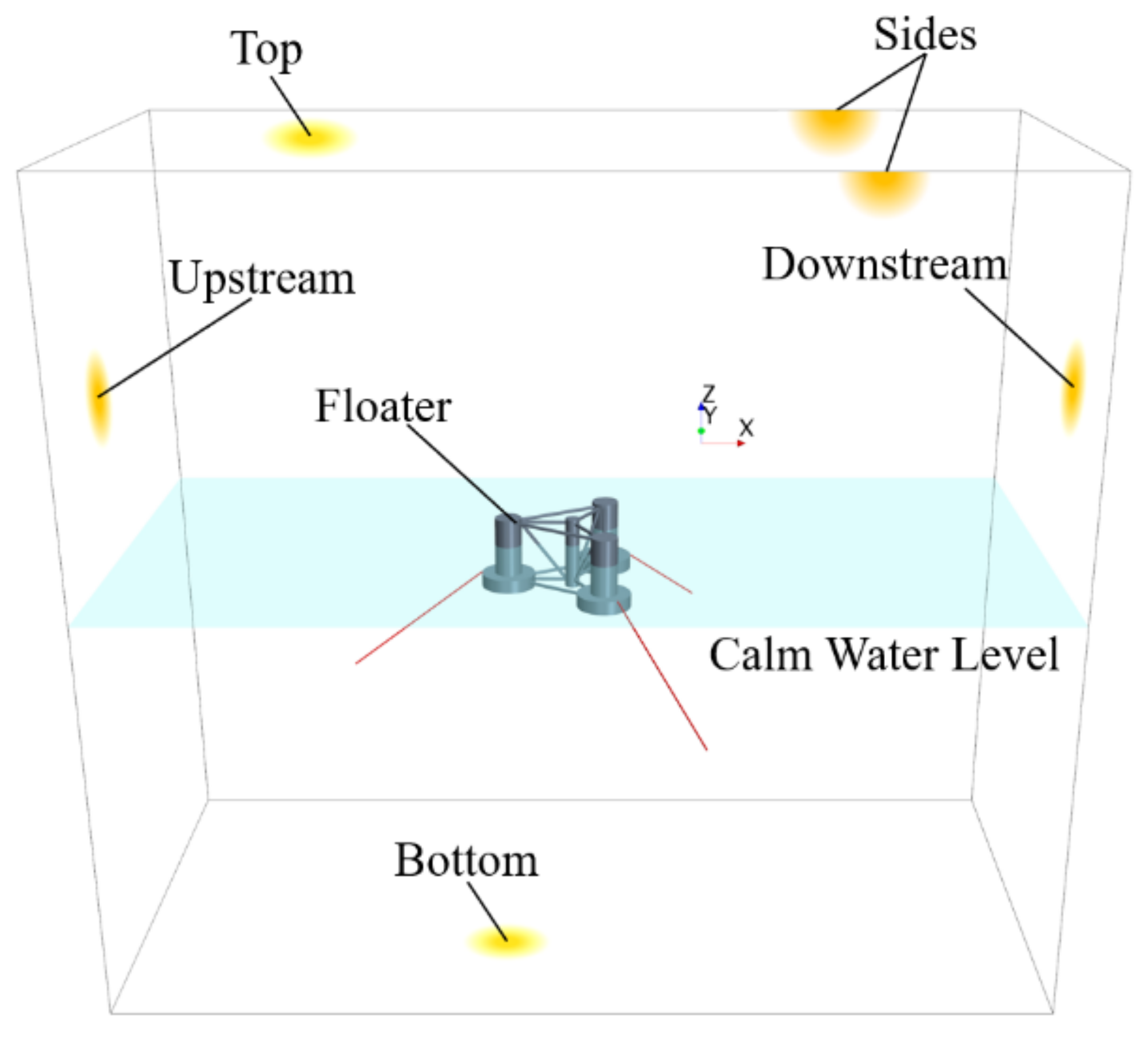
3.2. Numerical Domain, Initial Conditions, and Boundary Conditions
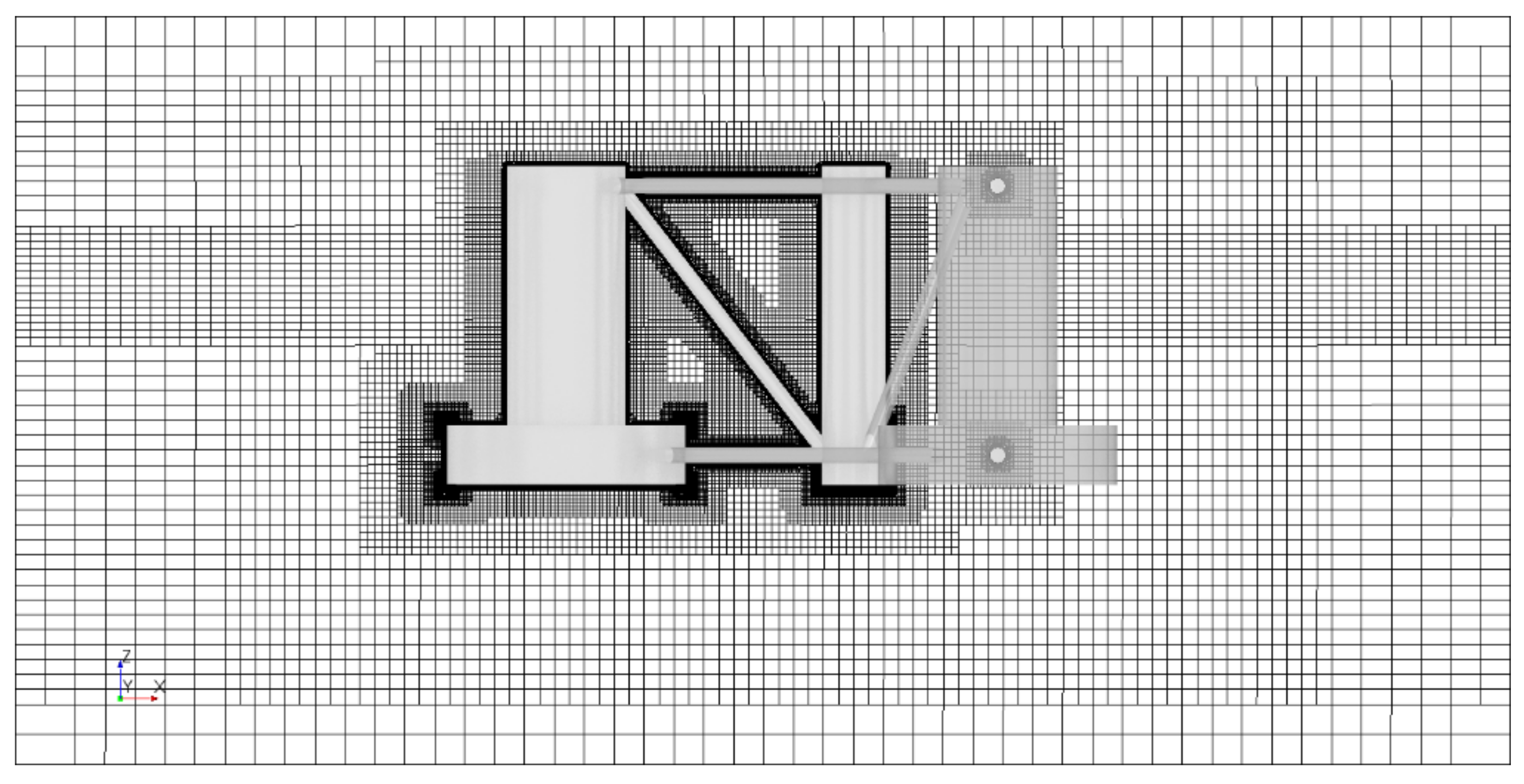
3.3. Computational Grid
3.4. Numerical Schemes and Settings
3.5. Model Parameter Tuning
4. Comparison of the Floater-Motion Time Series
5. Method of Analysis
5.1. Estimation of the Linear and Quadratic Damping Coefficients Using Analysis
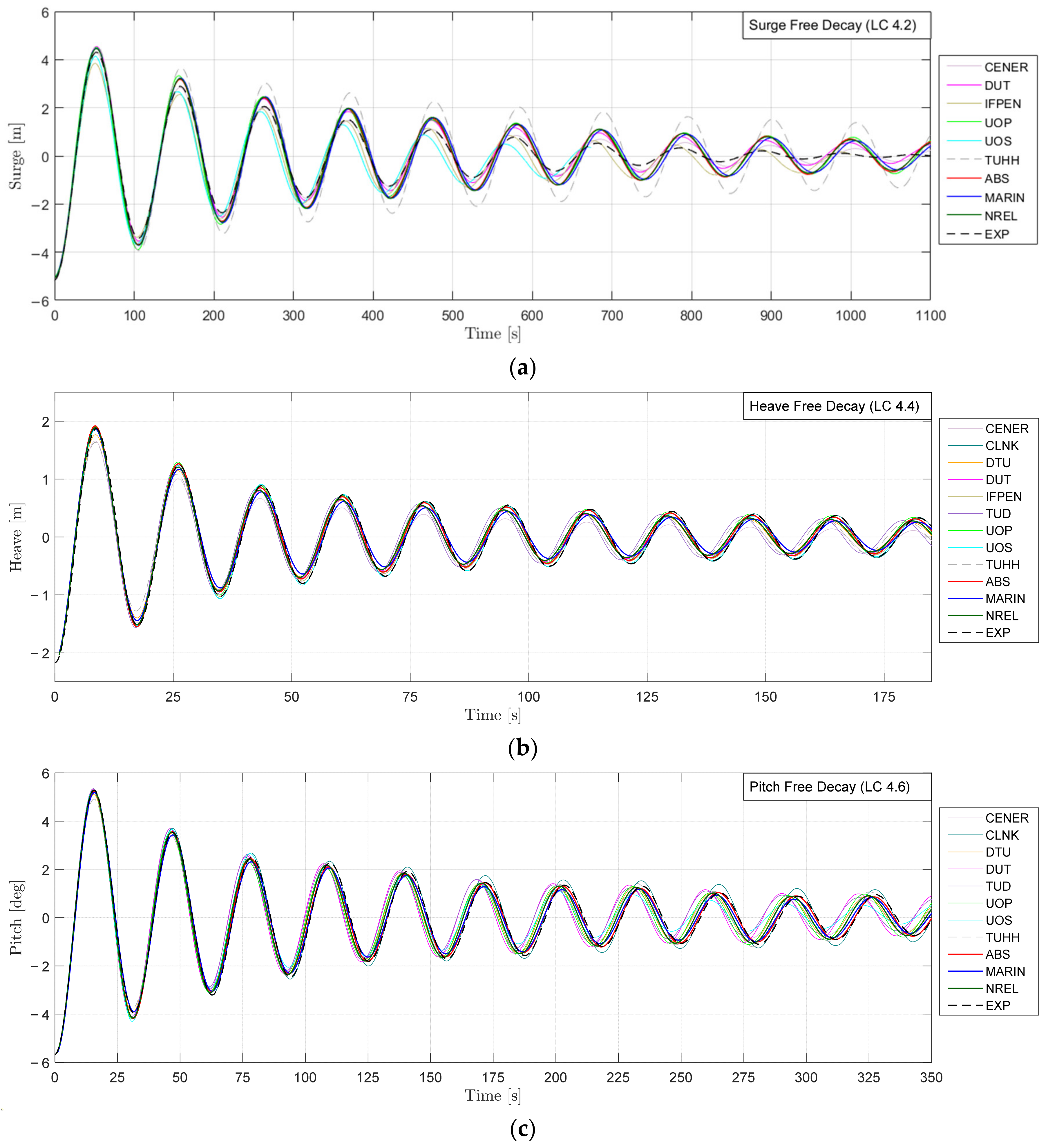
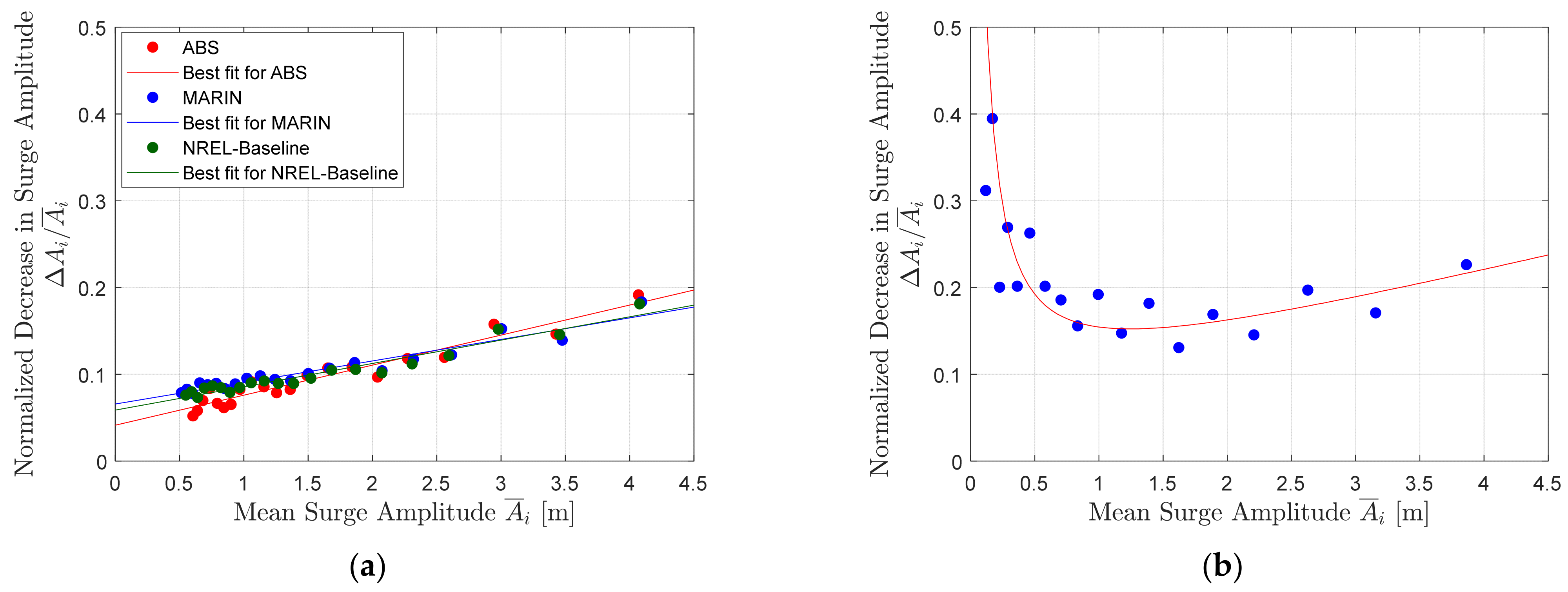
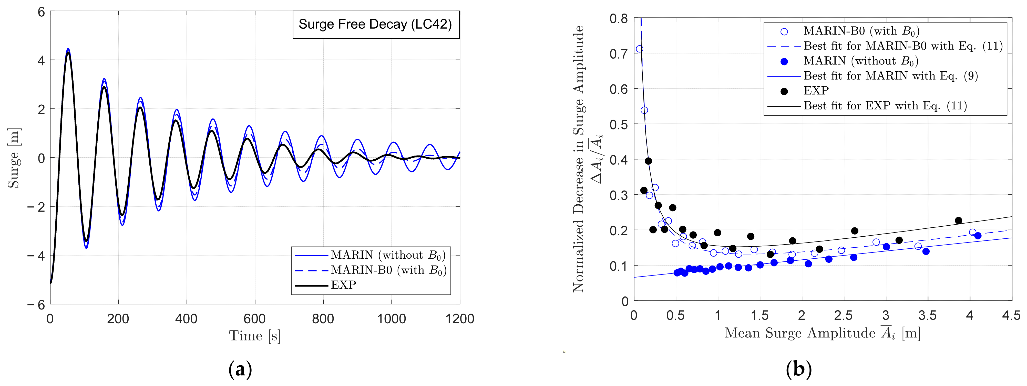
5.1.1. Surge Free Decay
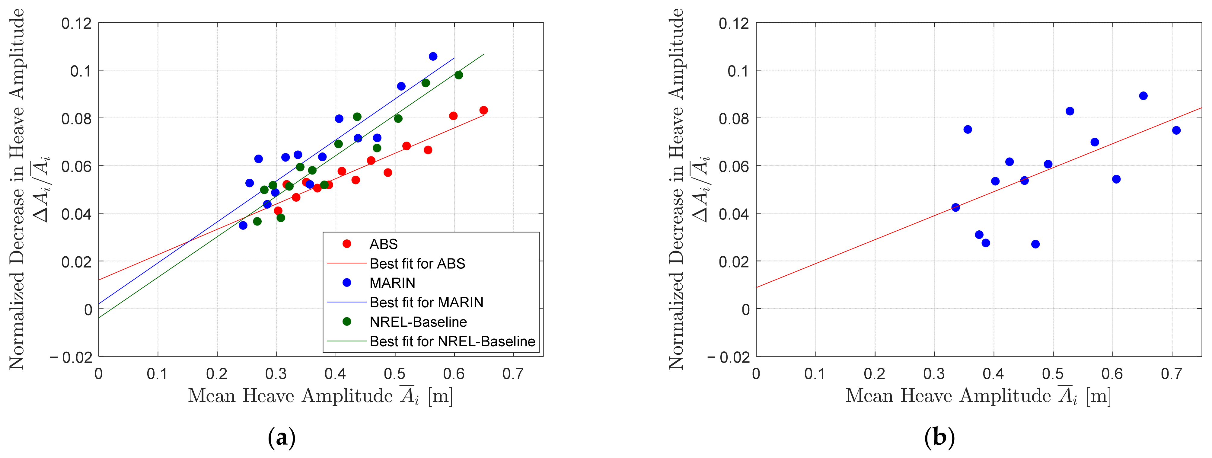
5.1.2. Heave Free Decay
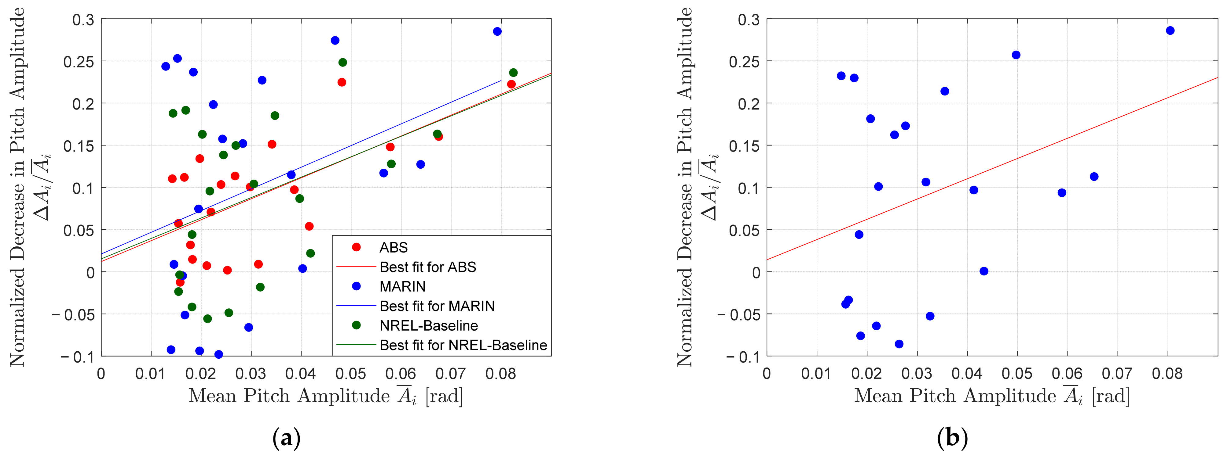
5.1.3. Pitch Free Decay
5.2. Equivalent Linear Damping Ratio
6. Estimation of Numerical Uncertainty
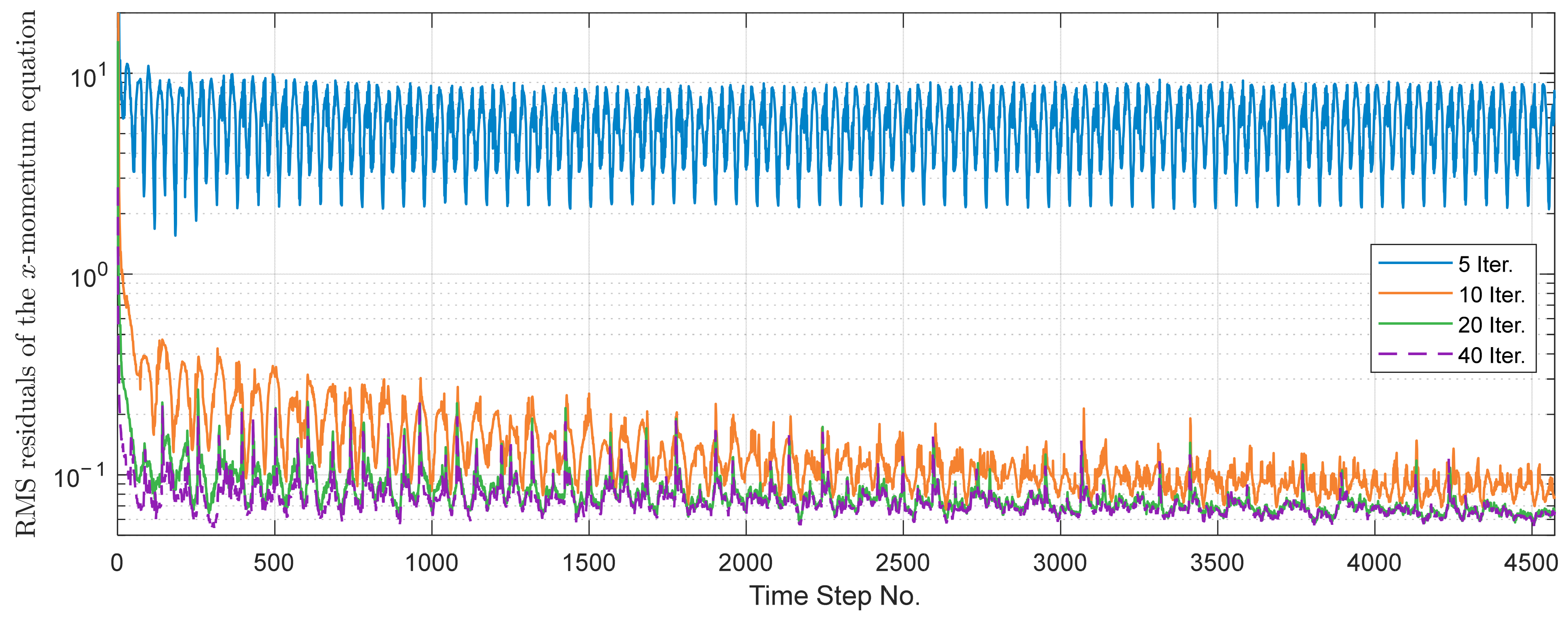
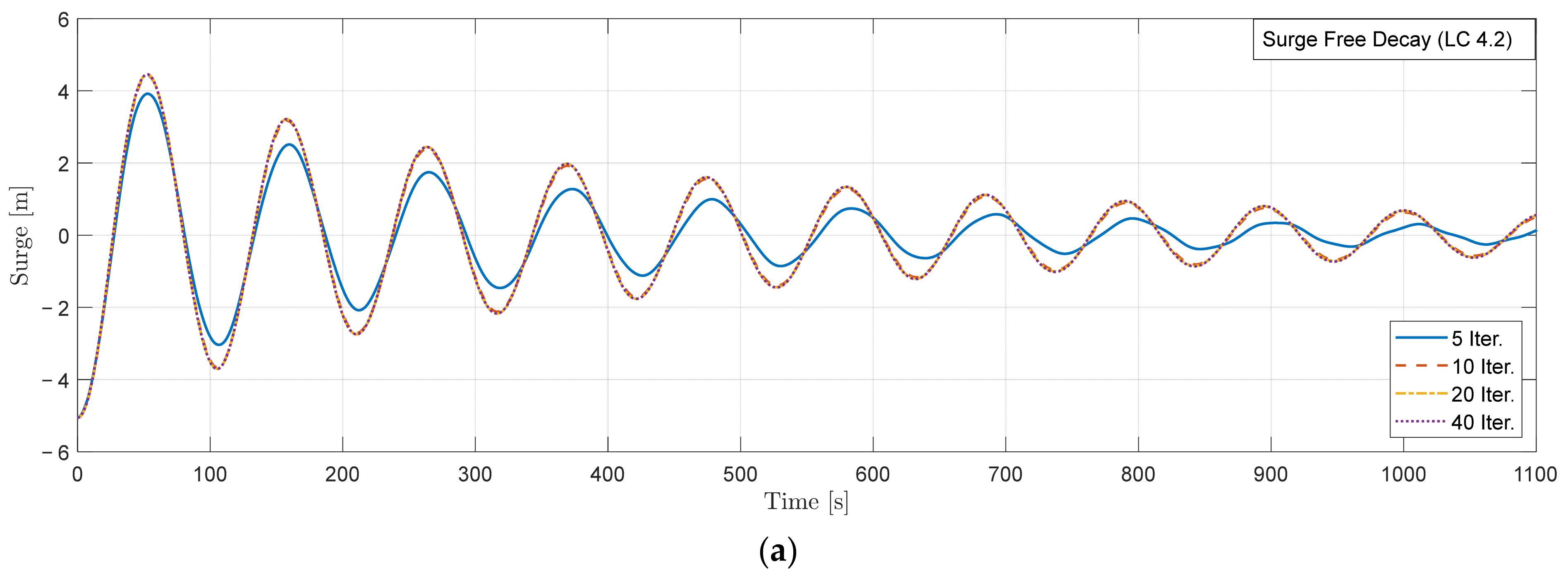
6.1. Iterative Uncertainty
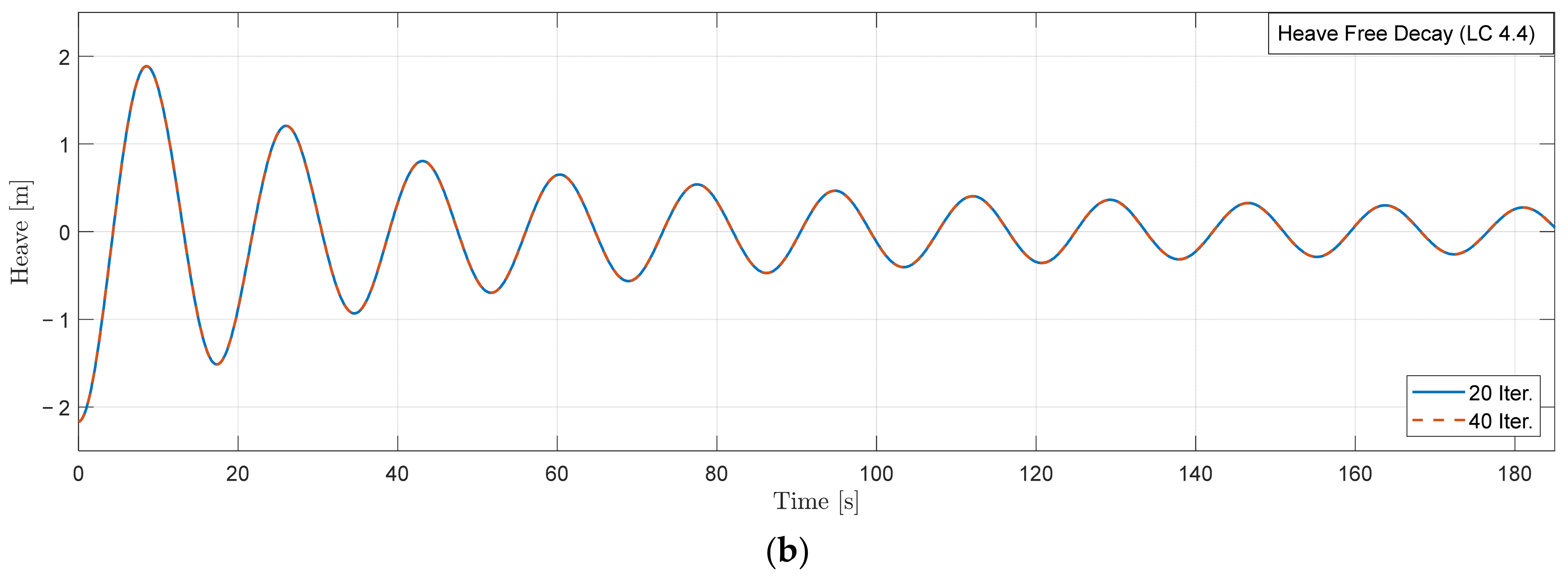
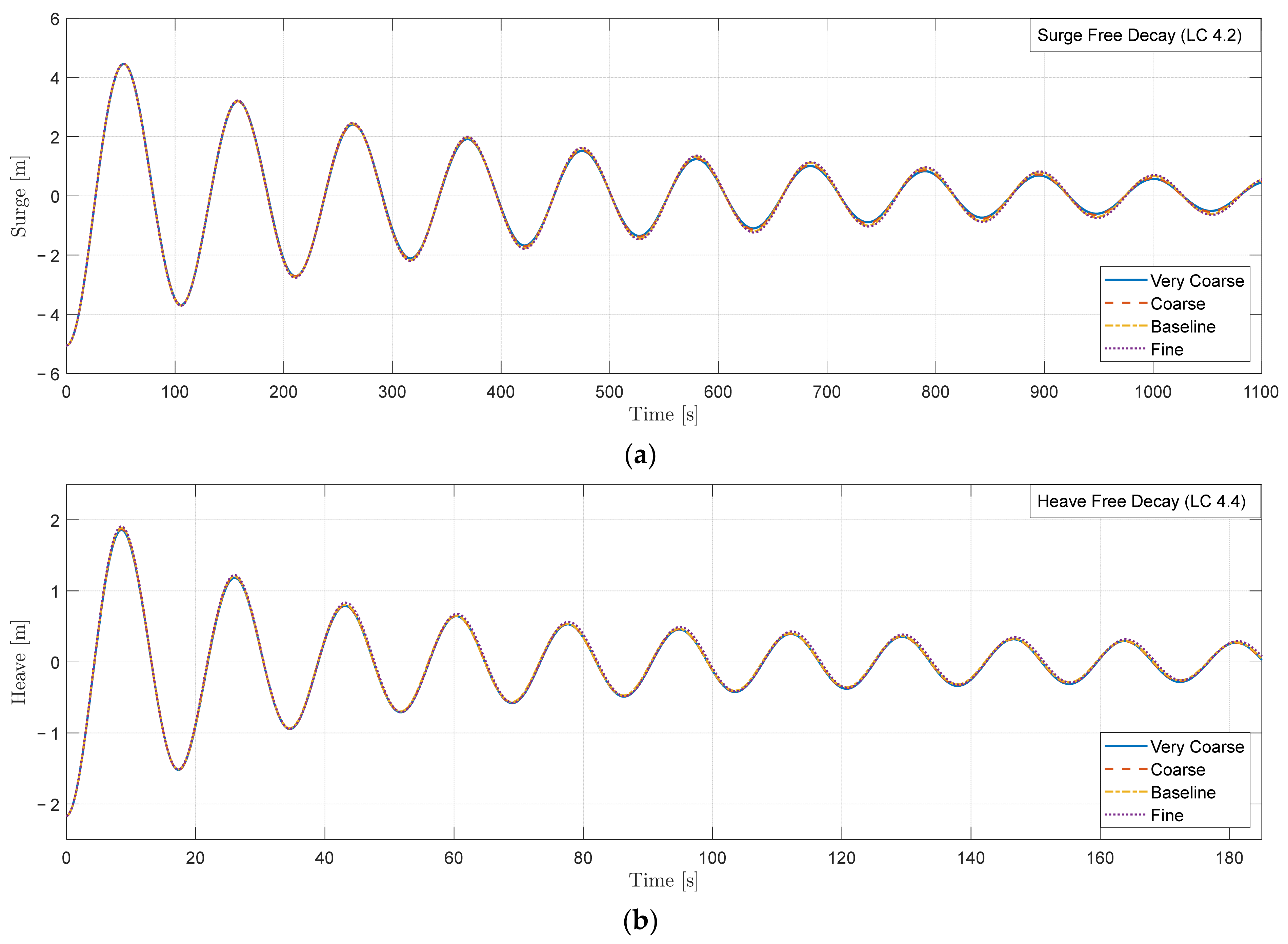
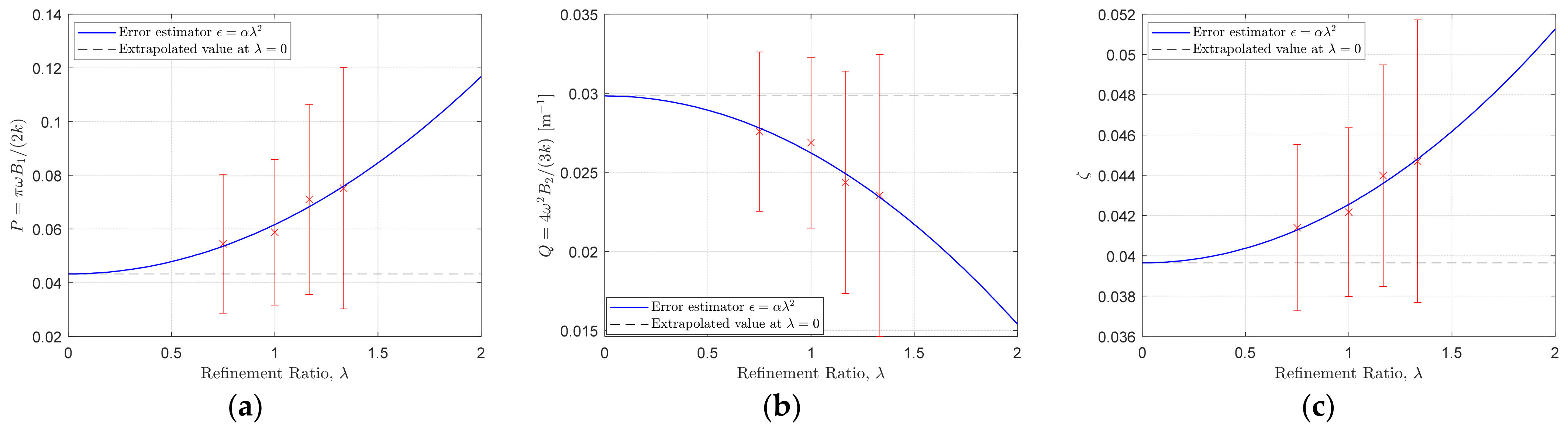
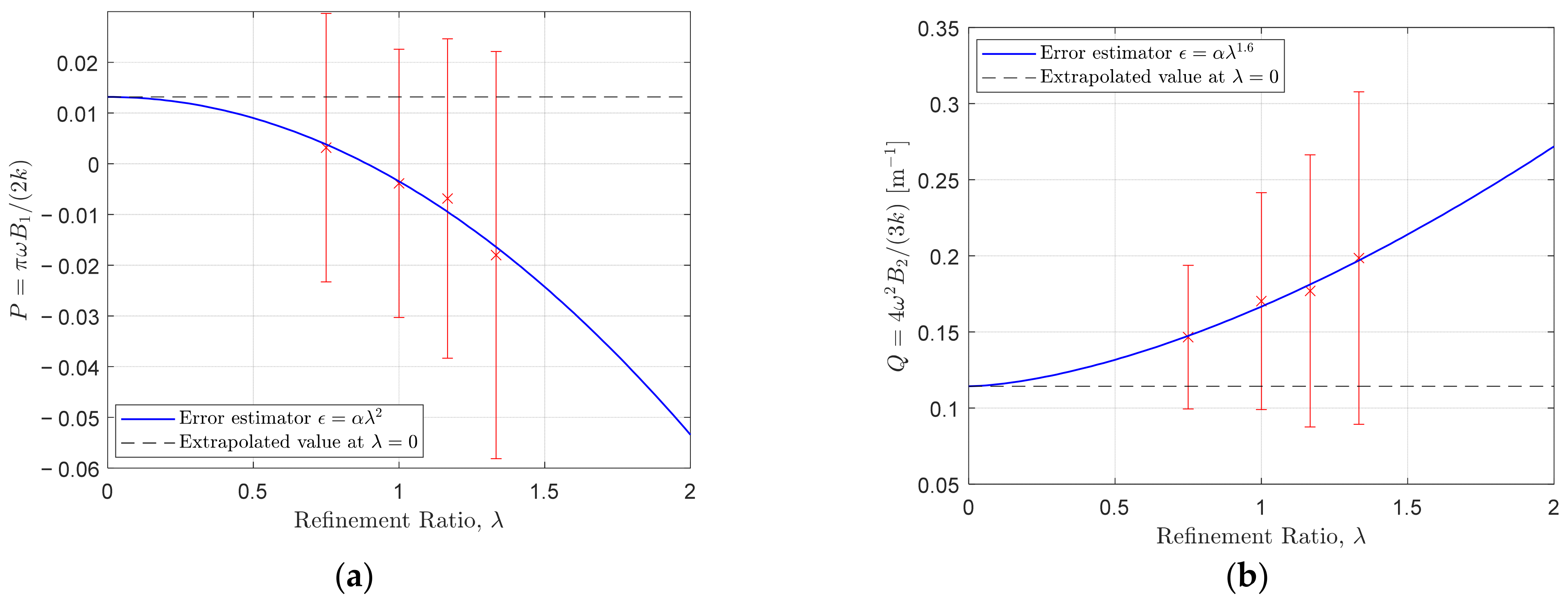
6.2. Discretization Errors and Uncertainties
6.3. Uncertainties from the Choice of Turbulence Models
7. Cross-Verification and Validation of the Numerical Results
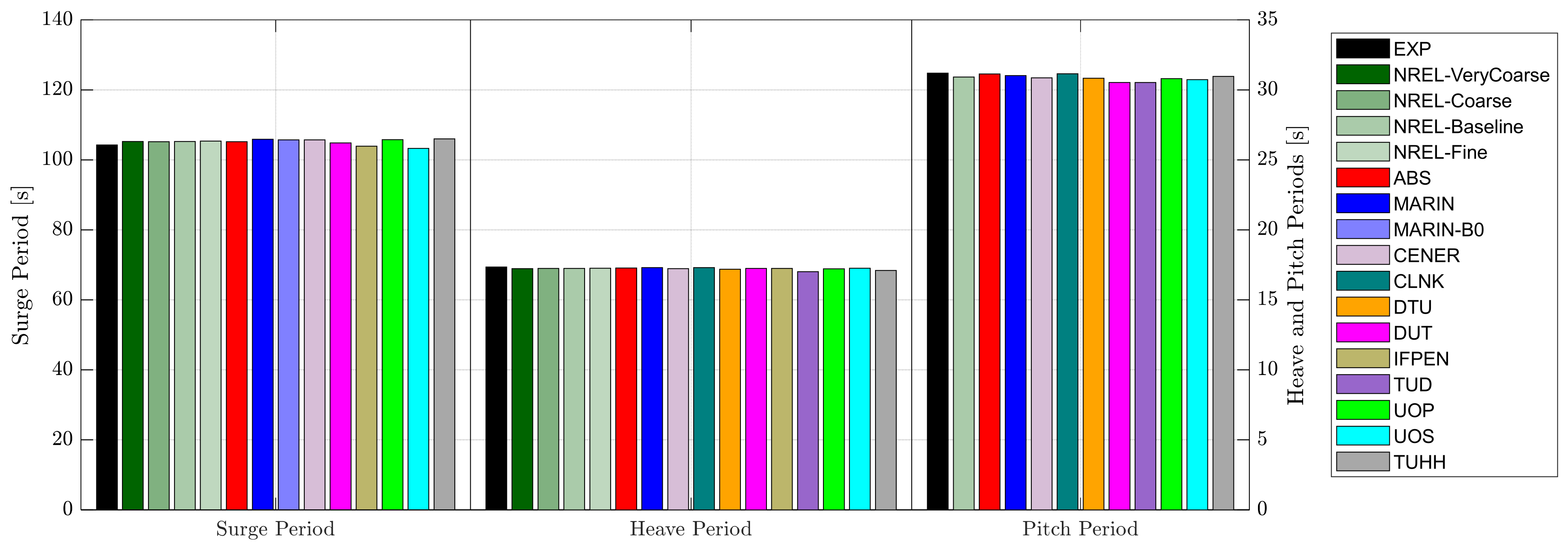
7.1. Motion Periods
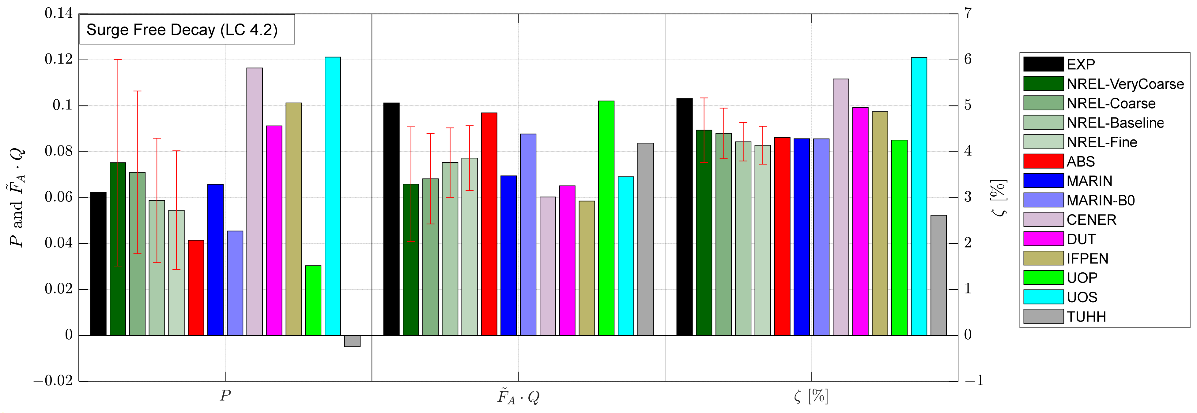
7.2. Surge Damping
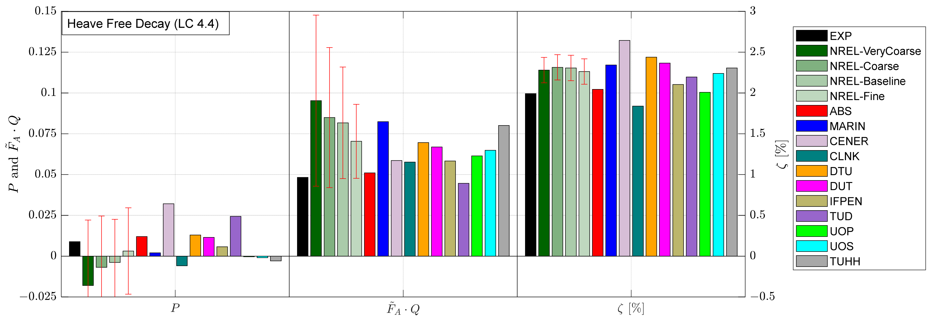
7.3. Heave Damping
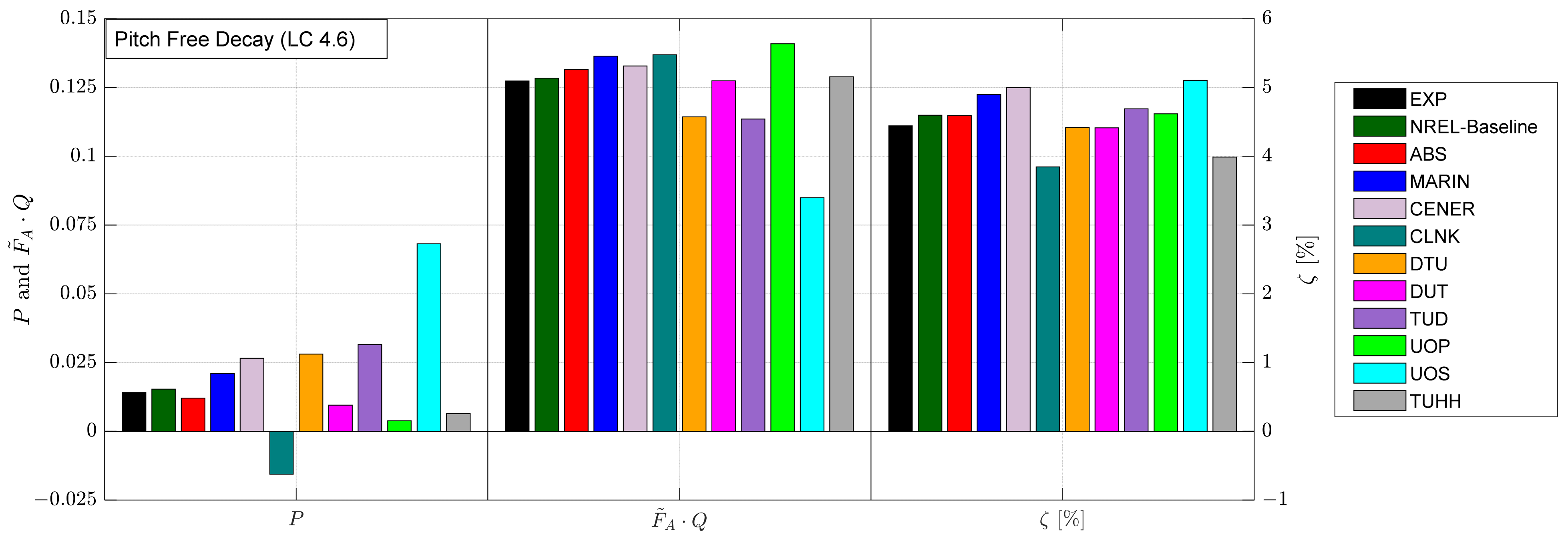
7.4. Pitch Damping
8. Conclusions
- A constant Coulomb-friction-type mechanical damping force was identified from the experimentally measured surge motion using a new modified analysis that also includes a constant damping force. The validity of the procedure was confirmed numerically by repeating the surge-decay CFD simulation with an added constant damping force, which was then successfully recovered from the numerical motion time series using the modified method.
- For selected CFD solutions, the discretization uncertainties were directly evaluated for the linear and quadratic damping coefficients and the equivalent linear damping ratio, which are the primary metrics that we would like to obtain from the CFD simulations to support the engineering modeling effort. This contrasts with previous efforts, which have typically focused on uncertainty estimates for more fundamental physical quantities, rather than the heavily postprocessed quantities such as damping coefficients.
- In the present analysis, even with the finest mesh of 25.6 million cells and the smallest time step of 533 steps per period, the estimated discretization uncertainty remains substantial, especially for the separate linear and quadratic damping coefficients.
- The grid resolution is the leading contributor to the discretization error, whereas the temporal discretization error is secondary, at least for surge decay.
- The numerical iterative errors and modeling uncertainties associated with the choice of turbulence model were also estimated but were found to be secondary to the discretization uncertainty for the load cases investigated and the numerical setup adopted.
- Interestingly, the linear and quadratic damping tend to show opposite trends as the simulation is refined, resulting in a very consistent equivalent linear damping ratio. This trend can also be observed when comparing across the CFD solutions of the OC6 participants, with the equivalent linear damping ratio being the most consistent across simulations.
- As a result, the equivalent linear damping ratio is the preferred metric against which mid-fidelity engineering models based on potential-flow theory and/or the Morison equation should be tuned; however, it does not provide information on the exact composition of the linear and quadratic damping.
- With all three load cases investigated, wave radiation plays a negligible role in the overall motion damping because of the low natural frequencies.
- The damping in the heave and pitch directions is predominantly quadratic, most likely coming from the drag force on the heave plates.
- On the other hand, the surge damping can have comparable contributions from linear and quadratic damping when the KC number is small, with the former primarily coming from the viscous boundary layer.
- Because wave-radiation damping is negligible compared to the viscous damping, the accuracy of the mid-fidelity models in predicting free-decay motion is almost exclusively determined by the tunning of the drag coefficients.
- The predominantly quadratic heave and pitch damping can be modeled satisfactorily with a quadratic empirical drag force on the heave plates, as demonstrated by the TUHH solution in the present investigation.
- For surge decay, however, the conventional form of the Morison equation without a linear drag term is fundamentally incorrect especially for low KC numbers. Either additional linear damping or a generalized Morison equation with a linear drag term should be used with mid-fidelity engineering models to model surge decay properly.
- Apart from not being able to capture the linear damping in surge, the mid-fidelity potential-flow model of TUHH generates mostly consistent predictions compared to the CFD simulations and shows a similar level of agreement with the experiment. The computing time, in terms of core hours, of a free-decay simulation using a typical mid-fidelity model is approximately 1/105 that of the corresponding CFD simulation. However, mid-fidelity potential-flow models are not fully predictive, and their accuracy strongly depends on the empirical drag coefficients used, which need to be tuned against some reference data. Therefore, to leverage the high efficiency of the mid-fidelity models fully, it is crucial to be able to obtain valid reference data from high-fidelity CFD simulations to help tune the model drag coefficients, especially during the initial design stage when the floater design is subject to frequent changes. This is, in fact, the primary goal of the present investigation.
Author Contributions
Funding
Data Availability Statement
Acknowledgments
Conflicts of Interest
Appendix A

| Group | CFD Software | Temporal Scheme | Spatial Schemes | Interface Capturing Scheme |
|---|---|---|---|---|
| ABS | OpenFOAM Ver. 2006 | VOF: Crank-Nicolson; Others: 2nd order implicit | Gradient: Gauss linear; Divergence (momentum/turbulence): Gauss limitedLinear; Divergence (other): Gauss linear; Laplacian: Gauss linear corrected | MULES |
| CENER | OpenFOAM Ver. 1812 | 1st order implicit | Gradient: cellLimited Gauss linear 1; Divergence (momentum/turbulence): Gauss linearUpwind; Divergence (other): Gauss linear; Laplacian: Gauss linear corrected | MULES; Gauss vanLeer |
| CLNK | OpenFOAM Ver. 2006 | 2nd order implicit | Gradient: cellLimited Gauss linear 1; Divergence (momentum/turbulence): Gauss linear; Divergence (other): Gauss linear; Laplacian: Gauss linear corrected | MULES; Gauss vanLeer |
| DTU | OpenFOAM Ver. 1912 | Equal blending of first and second order implicit | Gradient: cellLimited Gauss linear 1; Divergence (momentum): Gauss vanLeer; Divergence (turbulence): Gauss upwind; Laplacian: Gauss linear corrected | MULES; Gauss vanLeer |
| DUT | STAR-CCM+ Ver. 14.06.013 | 2nd order implicit | 2nd order hybrid-BCD for convection; 2nd order hybrid Gauss-LSQ for gradient with Venkatakrishnan’s limiter; 2nd order upwind for turbulence quantities | HRIC |
| IFPEN | OpenFOAM Ver. 1812 | 1st order implicit | Gradient: Gauss linear; Divergence (momentum/turbulence): Gauss upwind; Divergence (other): Gauss linear; Laplacian: Gauss linear corrected | MULES; Gauss vanLeer |
| MARIN | ReFRESCO Ver. 2.7 | 2nd order implicit | 2nd order harmonic TVD scheme of Van Leer; Gaussian least-squares | ReFRICS [43] |
| NREL 1 | STAR-CCM+ Ver. 13.06.012 | 2nd order implicit | 2nd order hybrid-BCD for convection; 2nd order hybrid Gauss-LSQ for gradient with Venkatakrishnan’s limiter; 2nd order upwind for turbulence quantities | HRIC |
| TUD | OpenFOAM Ver. 2012 | 1st order implicit | Gradient: cellLimited Gauss linear 1; Divergence: Gauss linear; Laplacian (LC4.2): Gauss linear corrected; Laplacian (LC4.4/4.6): Gauss linear limited 0.33 | MULES; Gauss vanLeer |
| UOP | OpenFOAM Ver. 1906 | 1st order implicit | Turbulence quantities: Gauss linearUpwind; Other quantities: Gauss linear | MULES; Gauss MUSCL |
| UOS | OpenFOAM Ver. 4.0 | 1st order implicit | Gradient Gauss linear; Divergence: Gauss limitedLinearV 1; Laplacian: Gauss linear corrected | MULES; Gauss vanLeer01 |
| Group | Algorithm | Number of PISO Iterations | Residual Tolerance | Maximum Outer Iterations |
|---|---|---|---|---|
| ABS | PIMPLE | 2 | N/A | 6 |
| CENER | PIMPLE | 1 | N/A | 3 |
| CLNK | PISO | 3 | N/A | N/A |
| DTU | PISO | 3 | N/A | N/A |
| DUT | SIMPLE | N/A | N/A | 20 |
| IFPEN | PISO | 3 | N/A | N/A |
| MARIN | SIMPLE | N/A | 10−4 | 50 |
| NREL 1 | SIMPLE | N/A | N/A | 20 |
| TUD | PISO | 3 | N/A | N/A |
| UOP | PISO | 3 | N/A | N/A |
| UOS | PIMPLE | 2 | U: tol 10−9, relTol 10−3; p_rgh: tol 10−5, relTol 10−3 | 10 |
| Group | Time Step 1 | Cell Sizes at Free Surface 2 as Fractions of h = 6 m | Isotropic Cell/Patch Sizes Near the Floater as Fractions of h = 6 m | Prism Layers | ||||||
|---|---|---|---|---|---|---|---|---|---|---|
| Near Floater 3 | Columns and Heave Plates 4 | Heave-Plate Corners and Btm. of Main Column 5 | Floater Surface | No. of Layers | First Layer | Total Thickness | ||||
| ABS | T/250 | 1/6 | 1/15 | 1/4 | 1/8 | 1/32 | 1/16 | 6 | 0.04 m | 0.45 m |
| CENER | Adaptive: Co ≤ 15 at interface, Co ≤ 25 elsewhere | 1/4 | 1/8 | 1/4 | 1/16 | 1/64 | 1/16 | 10 | 0.01415 m | 0.48 m |
| CLNK | Adaptive: Co ≤ 1 everywhere | 1/0.6 | 1/10 | 1/4 | 1/40 | 1/40 | 1/40 | 5 | 0.145 m | 1.22 m |
| DTU | Adaptive: Co<5 | 1/8 | 1/8 | 1/6 | 1/8 | 1/32 | 1/16 | 7 | 0.005 m | 0.48 m |
| DUT | T/400 | 1/4 | 1/8 | 1/4 | 1/16 | 1/64 | 1/16 | 15 | 0.002 m | 0.48 m |
| IFPEN | Adaptive: Co ≤ 0.5 at interface, Co ≤ 2.5 elsewhere | 1/8 | 1/8 | 1/16 | 1/16 | 1/32 | 1/32 | 7 | 0.00566 m | 0.185 m |
| MARIN | T/400 | 1/4 | 1/8 | 1/4 | 1/16 | 1/16 | 1/16 | 15 | 0.002 m | 0.48 m |
| NREL 6 | T/400 | 1/4 | 1/8 | 1/4 | 1/16 | 1/64 | 1/16 | 15 | 0.002 m | 0.48 m |
| TUD | Adaptive: Co ≤ 1.5 | 1/4 | 1/4 | 3/4 | 1/8 | 1/32 | 1/16 | 9 | 0.05 m | 0.48 m |
| UOP | T/600 to T/750 | 1/8 | 1/8 | 1/4 | 1/64 | 1/64 | 1/64 | No prism layers | ||
| UOS | Tmin/600 | 1/4 | 1/8 | 1/8 | 1/8 | 1/16 | 1/16 | 8 | 0.02 m | 0.4 m |
| Group | Domain Size (Full Scale) | Wave-Damping Zone (Upstream/Downstream) | 6Dof Motion Solver Parameters | Dynamic Mesh | Turb. Model | |||||
|---|---|---|---|---|---|---|---|---|---|---|
| (m) | (m) | (m) | Half Domain (-Sym.) | Acceleration Relaxation (OpenFOAM) | Acceleration Damping (OpenFOAM) | DOF | ||||
| ABS | [−150, 190] | [−145, 145] | [−145, 145] | No | 72 m/100 m | N/A (ABS in-house) | N/A (ABS in-house) | 6 | Overset (ABS in-house) | SST k-ω |
| CENER | [−200, 200] | [−100, 100] | [−180, 180] | No | None | 1.0 | 1.0 | 6 | Morphing | SST k-ω |
| CLNK | [−200, 200] | [−100, 100] | [−180, 100] | No | 50 m/50 m | 0.6 | 1.0 | 6 | Morphing | SST k-ω |
| DTU | [−200, 200] | [−100, 100] | [−180, 180] | No | None | 0.95 | N/A | 6 | Morphing | SST k-ω |
| DUT | [−200, 200] | [−100, 100] | [−180, 180] | No | 50 m/50 m | N/A | N/A | 6 | Morphing | Spalart–Allmaras DES |
| IFPEN | [−210, 210] | [−120, 120] | [−180, 150] | No | None | 1.0 | 1.0 | 6 | Morphing | RNG k-ε |
| MARIN | [−200, 200] | [−100, 100] | [−180, 180] | No | 50 m/50 m | N/A | N/A | 6 | Morphing | SST k-ω |
| NREL 1 | [−200, 200] | [−100, 100] | [−180, 180] | No | 50 m/50 m | N/A | N/A | 6 | Morphing | Spalart–Allmaras DES |
| TUD | [−200, 200] | [−100, 100] | [−180, 180] | No | None | 1.0 | 1.0 | 6 | Morphing | SST k-ω |
| UOP | [−200, 200] | [−100, 100] | [−180, 180] | No | 50 m/50 m | 0.7 | 1.0 | 6 | Morphing | Spalart–Allmaras DES |
| UOS | [−200, 200] | [−100, 100] | [−180, 180] | No | 50 m/50 m | 0.7 | 1.0 | 6 | Morphing | None |
References
- Jonkman, J.M. The new modularization framework for the FAST Wind Turbine CAE Tool. In Proceedings of the 51st AIAA Aerospace Sciences Meeting including the New Horizons Forum and Aerospace Exposition, Grapevine, TX, USA, 7–10 January 2013. [Google Scholar] [CrossRef] [Green Version]
- Wang, L.; Robertson, A.; Jonkman, J.; Yu, Y.-H. Uncertainty assessment of CFD investigation of the nonlinear difference-frequency wave loads on a semisubmersible FOWT platform. Sustainability 2021, 13, 64. [Google Scholar] [CrossRef]
- Wang, L.; Robertson, A.; Jonkman, J.; Yu, Y.-H.; Koop, A.; Borràs Nadal, A.; Li, H.; Bachynski, E.; Pinguet, R.; Shi, W.; et al. OC6 Phase Ib: Validation of the CFD predictions of difference-frequency wave excitation on an FOWT semisubmersible. Ocean Eng. 2021, 241, 110026. [Google Scholar] [CrossRef]
- Wang, L.; Robertson, A.; Jonkman, J.; Yu, Y.-H.; Koop, A.; Borràs Nadal, A.; Li, H.; Shi, W.; Pinguet, R.; Zhou, Y.; et al. Investigation of nonlinear difference-frequency wave excitation on a semisubmersible offshore-wind platform with bichromatic-wave CFD simulations. In Proceedings of the ASME 2021 3rd International Offshore Wind Technical Conference, Boston, MA, USA, 16–17 February 2021. [Google Scholar] [CrossRef]
- Böhm, M.; Robertson, A.; Hübler, C.; Rolfes, R.; Schaumann, P. Optimization-based calibration of hydrodynamic drag coefficients for a semisubmersible platform using experimental data of an irregular sea state. J. Phys. Conf. Ser. 2020, 1669, 012023. [Google Scholar] [CrossRef]
- Robertson, A.; Jonkman, J.; Masciola, M.; Song, H.; Goupee, A.; Coulling, A.; Luan, C. Definition of the Semisubmersible Floating System for Phase II of OC4; National Renewable Energy Laboratory: Golden, CO, USA, 2014. Available online: https://www.nrel.gov/docs/fy14osti/60601.pdf (accessed on 24 September 2021).
- Robertson, A.; Wendt, F.; Jonkman, J.; Popko, W.; Dagher, H.; Gueydon, S.; Qvist, J.; Vittori, F.; Azcona, J.; Uzunoglu, E. OC5 Project Phase II: Validation of global loads of the DeepCwind floating semisubmersible wind turbine. Energy Procedia 2017, 137, 38–57. [Google Scholar] [CrossRef]
- Coulling, A.; Goupee, A.; Robertson, A.; Jonkman, J.; Dagher, H. Validation of a FAST semi-submersible floating wind turbine numerical model with DeepCwind test data. J. Renew. Sustain. Energy 2013, 5, 023116. [Google Scholar] [CrossRef]
- Robertson, A.; Gueydon, S.; Bachynski, E.; Wang, L.; Jonkman, J.; Alarcón, D.; Amet, E.; Beardsell, A.; Bonnet, P.; Boudet, B.; et al. OC6 Phase I: Investigating the underprediction of low-frequency hydrodynamic loads and responses of a floating wind turbine. J. Phys. Conf. Ser. 2020, 1618, 032033. [Google Scholar] [CrossRef]
- Robertson, A.; Bachynski, E.; Gueydon, S.; Wendt, F.; Schünemann, P. Total experimental uncertainty in hydrodynamic testing of a semisubmersible wind turbine, considering numerical propagation of systematic uncertainty. Ocean Eng. 2020, 195, 106605. [Google Scholar] [CrossRef]
- Tran, T.T.; Kim, D.H. The coupled dynamic response computation for a semi-submersible platform of floating offshore wind turbine. J. Wind Eng. Ind. Aerodyn. 2015, 147, 104–119. [Google Scholar] [CrossRef]
- Tran, T.T.; Kim, D.H. Fully coupled aero-hydrodynamic analysis of a semi-submersible FOWT using a dynamic fluid body interaction approach. Renew. Energy 2016, 92, 244–261. [Google Scholar] [CrossRef]
- Burmester, S.; Vaz, G.; el Moctar, O. Towards credible CFD simulations for floating offshore wind turbines. Ocean Eng. 2020, 209, 107237. [Google Scholar] [CrossRef]
- Eça, L.; Hoekstra, M. A procedure for the estimation of the numerical uncertainty of CFD calculations based on grid refinement studies. J. Comput. Phys. 2014, 262, 104–130. [Google Scholar] [CrossRef]
- Wang, Y.; Chen, H.-C.; Vaz, G.; Burmester, S. CFD simulation of semi-submersible floating offshore wind turbine under pitch decay motion. In Proceedings of the ASME 2019 2nd International Offshore Wind Technical Conference, St. Julian’s, Malta, 3–6 November 2019. [Google Scholar] [CrossRef]
- Wang, Y.; Chen, H.-C.; Koop, A.; Vaz, G. Verification and validation of CFD simulations for semi-submersible floating offshore wind turbine under pitch free-decay motion. Ocean Eng. 2021, 242, 109993. [Google Scholar] [CrossRef]
- Li, H.; Bachynski-Polić, E. Experimental and numerically obtained low-frequency radiation characteristics of the OC5-DeepCwind semisubmersible. Ocean Eng. 2021, 232, 109130. [Google Scholar] [CrossRef]
- Burmester, S.; Vaz, G.; Gueydon, S.; el Moctar, O. Investigation of a semi-submersible floating wind turbine in surge decay using CFD. Ship Technol. Res. 2020, 67, 2–14. [Google Scholar] [CrossRef]
- Burmester, S.; Vaz, G.; el Moctar, O.; Gueydon, S.; Koop, A.; Wang, Y.; Chen, H. High-fidelity modelling of floating offshore wind turbine platforms. In Proceedings of the ASME 2020 39th International Conference on Ocean, Offshore and Arctic Engineering, Fort Lauderdale, FL, USA, 3–7 August 2020. [Google Scholar] [CrossRef]
- Wang, Y.; Chen, H.-C.; Vaz, G.; Burmester, S. CFD simulation of semi-submersible floating offshore wind turbine under regular waves. In Proceedings of the 30th International Ocean and Polar Engineering Conference, Shanghai, China, 11–16 October 2020. [Google Scholar]
- Wang, Y.; Chen, H.-C.; Vaz, G.; Mewes, S. Verification study of CFD simulation of semi-submersible floating offshore wind turbine under regular waves. In Proceedings of the ASME 2021 3rd International Conference on Ocean, Offshore and Arctic Engineering, Boston, MA, USA, 16–17 February 2021. [Google Scholar] [CrossRef]
- Bozonnet, P.; Emery, A. CFD simulations for the design of offshore floating wind platforms encompassing heave plates. In Proceedings of the 25th International Ocean and Polar Engineering Conference, Kona, HI, USA, 21–26 June 2015. [Google Scholar]
- Zhang, Y.; Kim, B. A fully coupled computational fluid dynamics method for analysis of semi-submersible floating offshore wind turbines under wind-wave excitation conditions based on OC5 data. Appl. Sci. 2018, 8, 2314. [Google Scholar] [CrossRef] [Green Version]
- Gueydon, S.; van Alfen, R. MARINET2 OC6 Model-Tests: A Series of Tests Focusing on the Hydrodynamics of the OC5 Semisubmersible; Maritime Research Institute Netherlands: Wageningen, The Netherlands, 2018. [Google Scholar]
- Siemens PLM Software. Simcenter STAR-CCM+ User Guide; Version 13.06.012; Siemens PLM Software: Plano, TX, USA, 2018. [Google Scholar]
- Weller, H.G.; Tabor, G.; Jasak, H.; Fureby, C. A tensorial approach to computational continuum mechanics using object-oriented techniques. Comput. Phys. 1998, 12, 620–631. [Google Scholar] [CrossRef]
- ReFRESCO. Available online: www.refresco.org (accessed on 21 May 2021).
- Ferreira González, D.; Göttsche, U.; Netzband, S.; Abdel-Maksoud, M. Advances on simulations of wave-body interactions under consideration of the nonlinear free water surface. Ship Technol. Res. 2021, 68, 27–40. [Google Scholar] [CrossRef]
- Morison, J.; O’Brien, M.; Johnson, J.; Schaaf, S. The force exerted by surface waves on piles. J. Pet. Technol. 1950, 2, 149–154. [Google Scholar] [CrossRef]
- Hirt, C.W.; Nichols, B.D. Volume of Fluid (VOF) method for the dynamics of free boundaries. J. Comput. Phys. 1981, 39, 201–225. [Google Scholar] [CrossRef]
- Cifani, P.; Michalek, W.; Priems, G.; Kuerten, J.; van der Geld, C.; Geurts, B. A comparison between the surface compression method and an interface reconstruction method for the VOF approach. Comput. Fluids 2016, 136, 421–435. [Google Scholar] [CrossRef] [Green Version]
- Spalart, P.; Jou, W.-H.; Strelets, M.; Allmaras, S. Comments on the feasibility of LES for wings, and on a hybrid RANS/LES. In Advances in DNS/LES; Greyden Press: Columbus, OH, USA, 1997; pp. 137–147. [Google Scholar]
- Shur, M.; Spalart, P.; Strelets, M.; Travin, A. A hybrid RANS-LES approach with delayed-DES and wall-modelled LES capabilities. Int. J. Heat Fluid Flow 2008, 29, 1638–1649. [Google Scholar] [CrossRef]
- Spalart, P.; Deck, S.; Shur, M.; Squires, K.; Strelets, M.; Travin, A. A new version of detached eddy simulation, resistant to ambiguous grid densities. Theor. Comput. Fluid Dyn. 2006, 20, 181–195. [Google Scholar] [CrossRef]
- Ren, C.; Lu, L.; Cheng, L.; Chen, T. Hydrodynamic damping of an oscillating cylinder at small Keulegan-Carpenter numbers. J. Fluid Mech. 2021, 913, A36. [Google Scholar] [CrossRef]
- Kim, J.; Baquet, A.; Jang, H. Wave propagation in CFD-based numerical wave tank. In Proceedings of the ASME 2019 38th International Conference on Ocean, Offshore and Arctic Engineering, Glasgow, UK, 9–14 June 2019. [Google Scholar] [CrossRef]
- Helder, J.A.; Pietersma, M. UMaine-DeepCwind/OC4 Semi Floating Wind Turbine Repeat Tests; Maritime Research Institute Netherlands: Wageningen, The Netherlands, 2013. [Google Scholar]
- Eça, L.; Vaz, G.; Toxopeus, S.L.; Hoekstra, M. Numerical errors in unsteady flow simulations. J. Verif. Valid. Uncert. 2019, 4, 021001. [Google Scholar] [CrossRef]
- Wang, W.; Wu, M.; Palm, J.; Eskilsson, C. Estimation of numerical uncertainty in computational fluid dynamics simulations of a passively controlled wave energy converter. Proc. Inst. Mech. Eng. Part M J. Eng. Marit. Environ. 2018, 232, 71–84. [Google Scholar] [CrossRef] [Green Version]
- Eça, L.; Hoekstra, M. Evaluation of numerical error estimation based on grid refinement studies with the method of the manufactured solutions. Comput. Fluids 2009, 38, 1580–1591. [Google Scholar] [CrossRef]
- Menter, F. Two-equation eddy-viscosity turbulence modeling for engineering applications. AIAA J. 1994, 32, 1598–1605. [Google Scholar] [CrossRef] [Green Version]
- Bureau Veritas. Classification of Mooring Systems for Permanent and Mobile Offshore Units Rule Note NR 493; Bureau Veritas: Paris, France, 2021; Available online: https://erules.veristar.com/dy/data/bv/pdf/493-NR_2021-07.pdf (accessed on 21 September 2021).
- Klaij, C.M.; Hoekstra, M.; Vaz, G. Design, analysis and verification of a volume-of-fluid model with interface-capturing scheme. Comput. Fluids 2018, 170, 324–340. [Google Scholar] [CrossRef]


| Parameters | Value | Unit |
|---|---|---|
| 1.392 × 10⁴ | m3 | |
| Vertical Center of Buoyancy, VCB (from SWL 1) | −13.17 | m |
| Vertical Center of Gravity, VCG (from SWL) | −7.53 | m |
| 1.407 × 10⁷ | kg | |
| about CG 2 | 1.2898 × 10¹⁰ | kg-m2 |
| about CG | 1.2851 × 10¹⁰ | kg-m2 |
| about CG | 1.4189 × 10¹⁰ | kg-m2 |
| Lines | End Points | (m) | (m) | (m) |
|---|---|---|---|---|
| 1 | Fairlead (FL1) | −40.87 | 0.00 | −14.0 |
| Anchor (AC1) | −105.47 | 0.00 | −58.4 | |
| 2 | Fairlead (FL2) | 20.43 | −35.39 | −14.0 |
| Anchor (AC2) | 52.73 | −91.34 | −58.4 | |
| 3 | Fairlead (FL3) | 20.43 | 35.39 | −14.0 |
| Anchor (AC3) | 52.73 | 91.34 | −58.4 |
| Load Case | Surge (m) | Sway (m) | Heave (m) | Roll (deg) | Pitch (deg) | Yaw (deg) |
|---|---|---|---|---|---|---|
| 4.2—Surge Decay | −5.1 | 0.9 | 0.0 | 0.1 | 0.7 | 0.3 |
| 4.4—Heave Decay | 0.1 | −0.3 | −2.2 | 0.2 | 0.3 | 0.1 |
| 4.6—Pitch Decay | −2.1 | 0.1 | −0.1 | −0.1 | −5.7 | 0.0 |
| Load Case | Surge (m/s) | Sway (m/s) | Heave (m/s) | Roll (deg/s) | Pitch (deg/s) | Yaw (deg/s) |
|---|---|---|---|---|---|---|
| 4.2—Surge Decay | 0.0 | 0.0 | 0.0 | 0.0 | 0.0 | 0.0 |
| 4.4—Heave Decay | 0.0 | 0.0 | 0.0 | −0.1 | 0.0 | 0.0 |
| 4.6—Pitch Decay | −0.2 | 0.0 | 0.0 | 0.0 | 0.0 | 0.0 |
| Boundary | Location | Type | Velocity | Pressure | Phase Fraction |
|---|---|---|---|---|---|
| Floater | N/A | Wall | No slip | Zero normal gradient | Zero normal gradient |
| Upstream | m | Velocity Inlet | Zero | Zero normal gradient | : water |
| Downstream | m | Velocity Inlet | Zero | Zero normal gradient | : water |
| Sides | m | Wall | Free slip | Zero normal gradient | Zero normal gradient |
| Bottom | m | Velocity Inlet | Zero | Zero normal gradient | Water only |
| Top | m | Pressure Outlet | Extrapolated backflow dir. | Atmospheric | Air only |
| Refinement Zones | |||
|---|---|---|---|
| [−5 m, 5 m] | 1/4 | 1/4 | 1/8 |
| [−40 m, 20 m] | 1/2 | 1/2 | 1/4 |
| [−80 m, 30 m] | 1 | 1 | 1/2 |
| Refinement Zones | Range (m) | y Range (m) | Range (m) | |
|---|---|---|---|---|
| Near Floater | [−60, 46] | [−50, 50] | [−40, 20] | 1/4 |
| Main Column | [−7, 7] | [−4, 4] | [−22, 12] | 1/16 |
| Upstream Col.—Heave Plate | [−45, −13] | [−14, 14] | [−23, −11] | 1/16 |
| Starboard Col.—Heave Plate | [−2, 30] | [11, 39] | [−23, −11] | 1/16 |
| Port Col.—Heave Plate | [−2, 30] | [−39, −11] | [−23, −11] | 1/16 |
| Upstream Col.—Upper Part | [−38.5, −19.5] | [−7, 7] | [−11, 12] | 1/16 |
| Starboard Col.—Upper Part | [5, 24] | [18, 32] | [−11, 12] | 1/16 |
| Port Col.—Upper Part | [5, 24] | [−32, −18] | [−11, 12] | 1/16 |
| Floater Surface Mesh | N/A | N/A | N/A | 1/16 |
| Refinement Zones | Range (m) | Range (m) | |
|---|---|---|---|
| Bottom of the Main Column | [0, 4.25] | [−21, −13] | 1/64 |
| Top Edge of Heave Plates | [10.75, 13.25] | [−15.25, −12.75] | 1/64 |
| Bottom Edge of Heave Plates | [10.75, 13.25] | [−21.25, −18.75] | 1/64 |
| No. Iter. | ||||||
|---|---|---|---|---|---|---|
| Value | Difference | Value (m−1) | Difference | Value | Difference | |
| 5 | 0.112 | 97% | 0.0327 | 20% | 6.06% | 45% |
| 10 | 0.064 | 12% | 0.0265 | 3.5% | 4.32% | 2.9% |
| 20 | 0.059 | 3.4% | 0.0269 | 2.0% | 4.22% | 0.4% |
| 40 | 0.057 | N/A | 0.0274 | N/A | 4.20% | N/A |
| No. Iter. | ||||||
|---|---|---|---|---|---|---|
| Value | Difference | Value (m−1) | Difference | Value | Difference | |
| 20 | −0.0039 | 6% | 0.170 | 0.8% | 2.306% | 0.4% |
| 40 | −0.0041 | N/A | 0.171 | N/A | 2.313% | N/A |
| Case | Number of Cells | No. Iter. | |||
|---|---|---|---|---|---|
| Very Coarse | 4/3 | 8 m | 6.7 million | 20 | |
| Coarse | 7/6 | 7 m | 8.6 million | 20 | |
| Baseline | 1 | 6 m | 12.9 million | 20 | |
| Fine | 3/4 | 4.5 m | 25.6 million | 20 |
| Cases | ||||||
|---|---|---|---|---|---|---|
| Value | Discretization Uncertainty | Value (m−1) | Discretization Uncertainty | Value | Discretization Uncertainty | |
| Very Coarse | 0.075 | ±60% | 0.0235 | ±38% | 4.5% | ±16% |
| Coarse | 0.071 | ±50% | 0.0244 | ±29% | 4.4% | ±13% |
| Baseline | 0.059 | ±47% | 0.0269 | ±21% | 4.2% | ±10% |
| Fine | 0.055 | ±48% | 0.0276 | ±19% | 4.1% | ±10% |
| Cases | ||||||
|---|---|---|---|---|---|---|
| Value | Discretization Uncertainty 1 | Value (m−1) | Discretization Uncertainty | Value | Discretization Uncertainty | |
| Very Coarse | −0.018 | ±0.04 | 0.20 | ±55% | 2.28% | ±7% |
| Coarse | −0.007 | ±0.04 | 0.18 | ±51% | 2.31% | ±7% |
| Baseline | −0.004 | ±0.03 | 0.17 | ±42% | 2.31% | ±7% |
| Fine | +0.003 | ±0.03 | 0.15 | ±33% | 2.26% | ±7% |
| Surge Damping | Heave Damping | |||||
|---|---|---|---|---|---|---|
| (m−1) | (%) | (m−1) | (%) | |||
| SA-DES 1 (Baseline) | 0.059 | 0.0269 | 4.22 | −0.004 | 0.170 | 2.31 |
| 0.061 | 0.0272 | 4.29 | −0.001 | 0.169 | 2.38 | |
| No Turbulence Model | 0.057 | 0.0290 | 4.34 | −0.004 | 0.171 | 2.31 |
| Max. Difference Relative to Baseline | 3.3% | 8.0% | 2.9% | 0.003 3 | 0.9% | 3.1% |
Publisher’s Note: MDPI stays neutral with regard to jurisdictional claims in published maps and institutional affiliations. |
© 2022 by the authors. Licensee MDPI, Basel, Switzerland. This article is an open access article distributed under the terms and conditions of the Creative Commons Attribution (CC BY) license (https://creativecommons.org/licenses/by/4.0/).
Share and Cite
Wang, L.; Robertson, A.; Jonkman, J.; Kim, J.; Shen, Z.-R.; Koop, A.; Borràs Nadal, A.; Shi, W.; Zeng, X.; Ransley, E.; et al. OC6 Phase Ia: CFD Simulations of the Free-Decay Motion of the DeepCwind Semisubmersible. Energies 2022, 15, 389. https://doi.org/10.3390/en15010389
Wang L, Robertson A, Jonkman J, Kim J, Shen Z-R, Koop A, Borràs Nadal A, Shi W, Zeng X, Ransley E, et al. OC6 Phase Ia: CFD Simulations of the Free-Decay Motion of the DeepCwind Semisubmersible. Energies. 2022; 15(1):389. https://doi.org/10.3390/en15010389
Chicago/Turabian StyleWang, Lu, Amy Robertson, Jason Jonkman, Jang Kim, Zhi-Rong Shen, Arjen Koop, Adrià Borràs Nadal, Wei Shi, Xinmeng Zeng, Edward Ransley, and et al. 2022. "OC6 Phase Ia: CFD Simulations of the Free-Decay Motion of the DeepCwind Semisubmersible" Energies 15, no. 1: 389. https://doi.org/10.3390/en15010389