
A Review of Modelling of the FCC Unit—Part II: The Regenerator


Abstract
:1. Introduction
2. FCC Regenerator
2.1. Regenerator Kinetics

| Authors | Conditions and Fuels Burned | Model/Correlation | ||||
|---|---|---|---|---|---|---|
| [21] | ✓ | Artificial graphite, coal char granules | ||||
| [25] | ✓ | ✓ | ✓ | Coked silica–alumina catalyst | ||
| [42] | ✓ | N/A | ||||
| [26] | ✓ | Coked Zeolite CDY, Alkaline ex-change zeolites , Transition metal exchanged zeolite | ||||
| [27] | ✓ | Coked Zeolites CRC-1, Y-7, Y-9 | ||||
| [41] | ✓ | ✓ | Coked Zeolite catalyst | |||
| [28] | ✓ | ✓ | ✓ | Coked OCTYDINE 1169 BR catalyst | ||
| [43] | ✓ | partial pressure Charcoal, graphite, coked FCC catalyst | ||||
| [44] | ✓ | Coked catalyst |
2.2. Hydrodynamics of the Regenerator
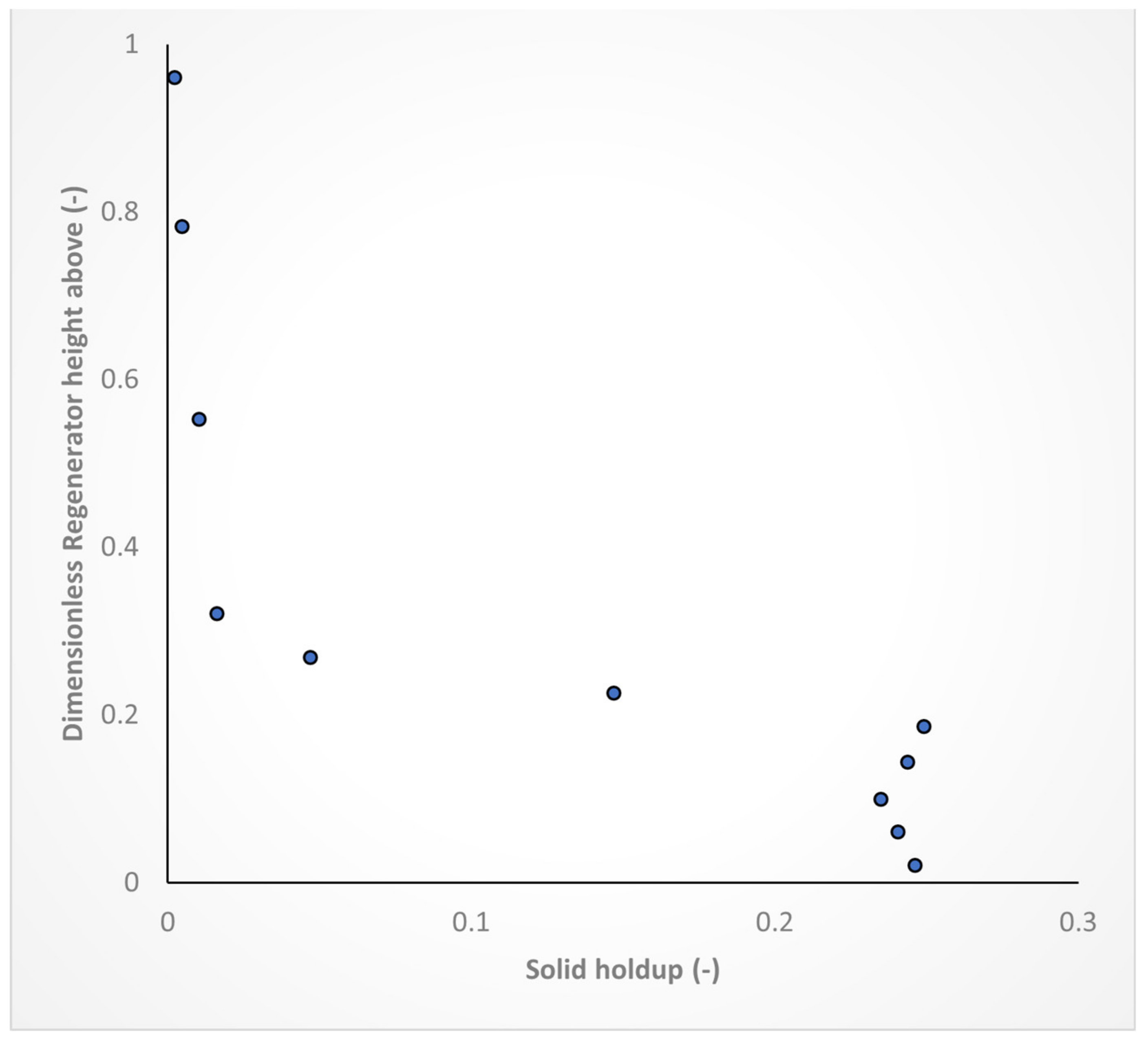
2.2.1. Axial Profiles
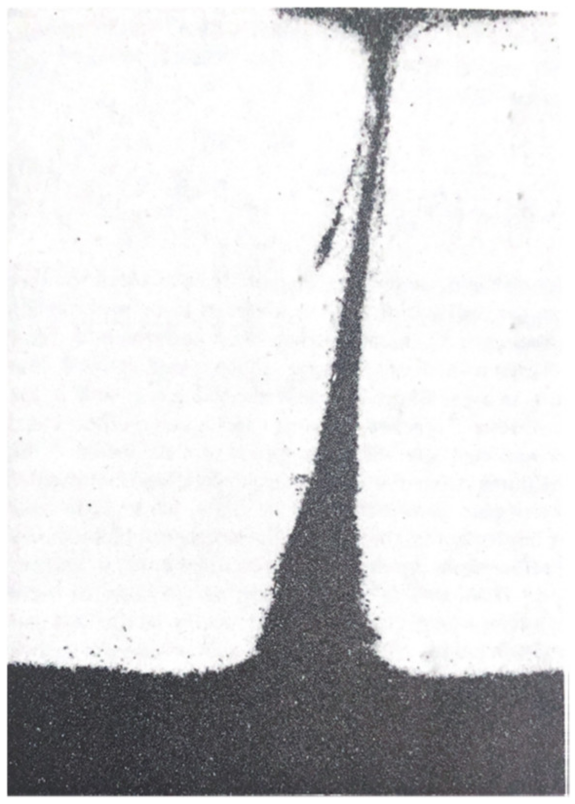
2.2.2. Bubbling Behaviour
2.3. Reactor Models for Bubbling Beds
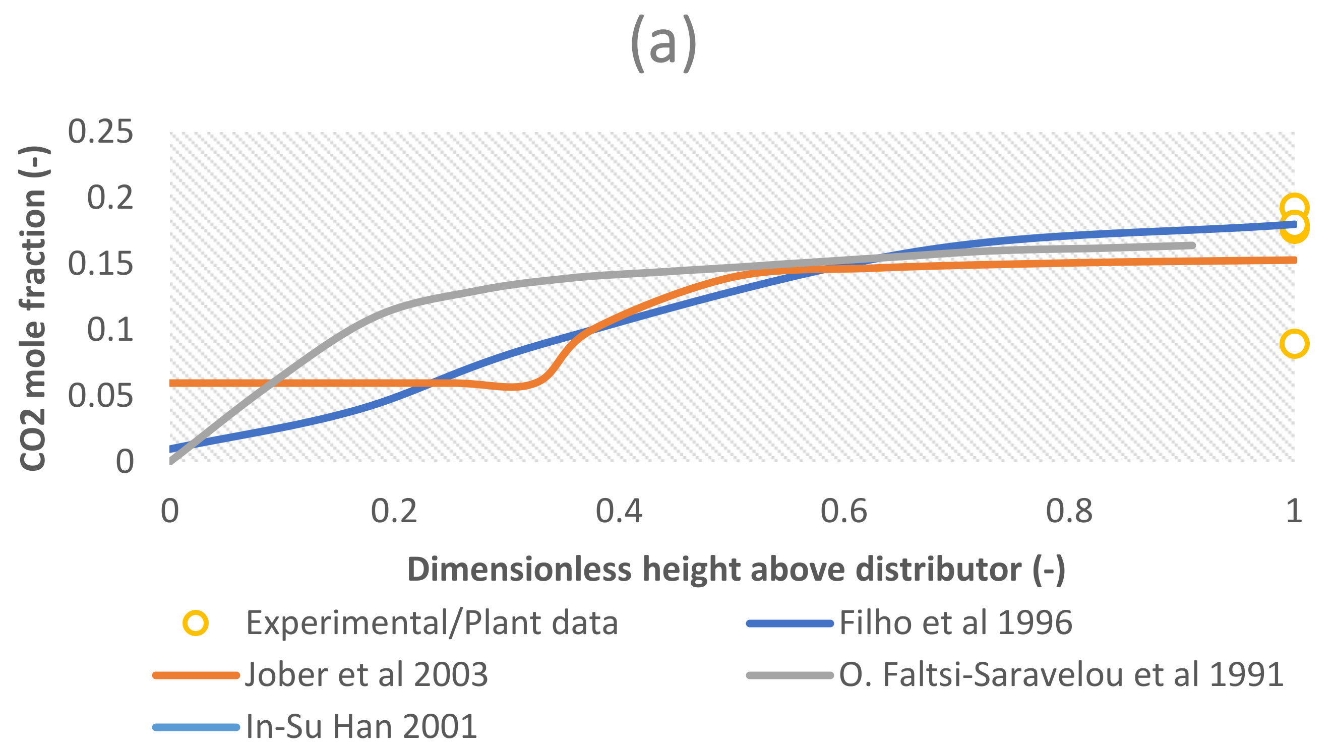
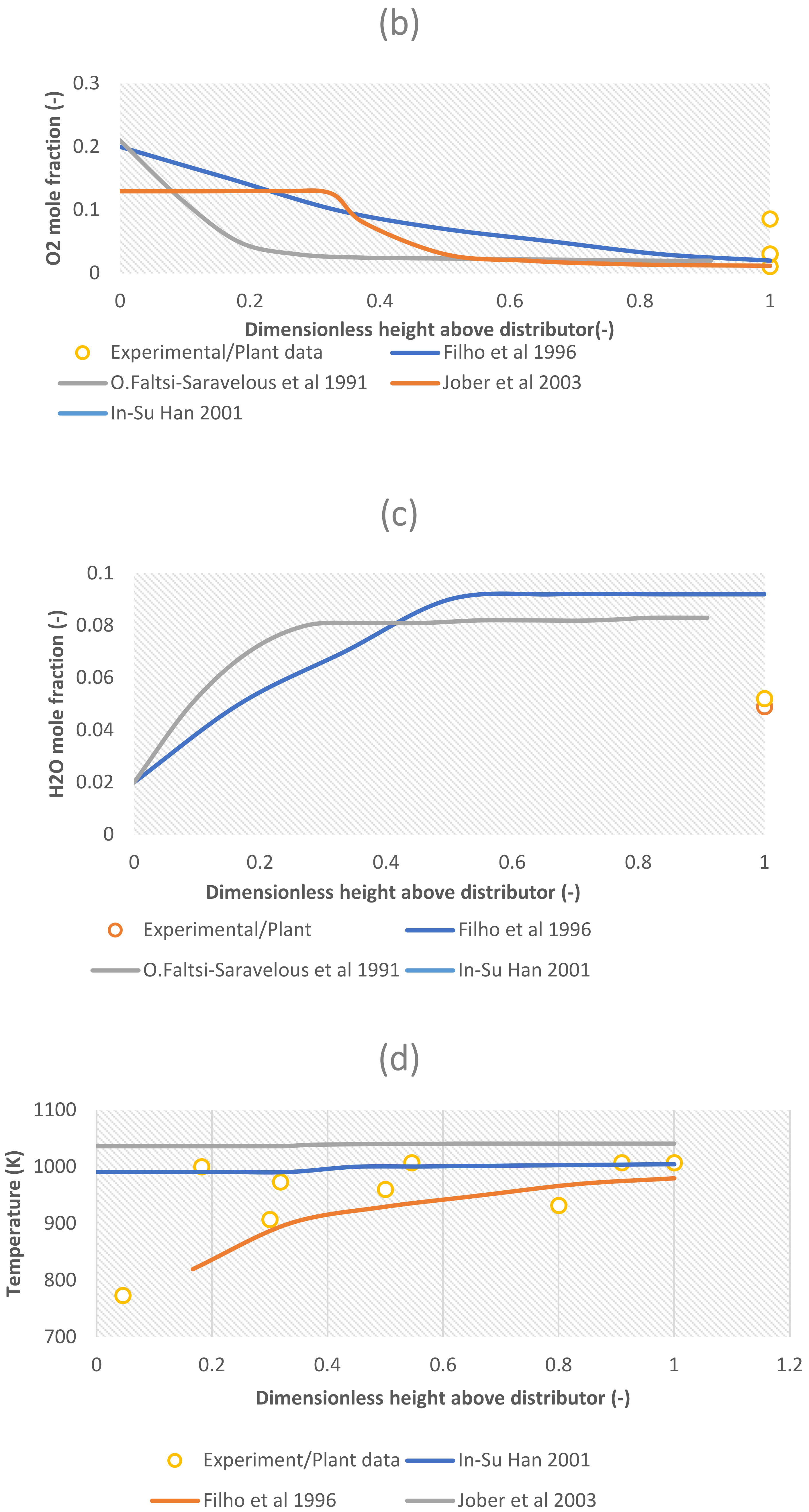
2.4. FCC Regenerator Performance Predictions
2.5. Shortcomings and Future Recommendations
- (a)
- Axial mixing: Table 4 shows that the mixing of solids and gas in the bed is usually assumed to be either plug flow or well mixed in the axial direction. Considering the results from Callcott et al. [104] that showed that tracer solids could be completely mixed in the axial direction in 75 s, and also noting that the characteristic residence time for solids in the FCC regenerator is in the range of minutes to an hour (see Table 1), then it is totally reasonable to assume complete mixing for solids in the axial direction. However, gas mixing is more complex, as was explained earlier. It has now been established that the motion of bubbles up the bed causes a rise to circulation patterns of solids in the bed so that solids are moving up the bed in bubbling regions and moving down the bed in regions of low bubbling activity. It was suggested by several workers [16,148] that the regions of downflow of solids drag down the interstitial gas so that downflow of gas is possible in the bed. Stephens et al. [16] suggested that the downflow of gas occurs when the downflow velocity of solids exceeds the velocity of rising emulsion gas. Consequently, this is what has led to back-mixing models for bubbling fluidised beds. The review in Table 4 shows that back-mixing models and their applicability to the FCC regenerator has yet to be explored, and since it has been clear from Levenspiel [142] that plug flow or well-mixed assumptions do not accurately predict gas mixing in the dense bed, it is worth exploring back-mixing models for their performance in describing gas flow in FCC dense beds;
- (b)
- Radial mixing: According to Grace [141], knowledge of lateral/axial mixing can be far more important than axial mixing in predicting the performance of fluidised units. The FCC regenerator models reviewed in Table 4 are all 1-D models that assume perfect axial mixing of both solids and gases so that any variation that occurs is only in the axial direction. It was described [104] that solids mixing is poor in the lateral (or radial) direction and that complete mixing is only achieved in the time scale in the order of , which exceeds the normal time scale for the residence time of solids in the FCC regenerator (see Table 1). Therefore, it seems unreasonable to assume perfect radial mixing of solids in the regenerator. In order to understand lateral/radial solid mixing better, a lateral dispersion coefficient was used to encompass all the solids mixing processes identified by Rowe and other workers [72,73,149] i.e., emulsion drift, bubble wake lift and bubble eruption scattering. Determination of the dispersion coefficient was generally performed in two ways; (i) a diffusion-type [101,150], where experimental data are fitted to a model that is based on the analogy that solid particles behave similar to gas molecules travelling in a continuous isotropic environment, and (ii) a stochastic-type model [105,151,152] that assumes a solid particle in a bubble induced mixing cell can randomly jump between adjacent mixing cells, and that this jumping is governed by a probability distribution. There has been some success in using these dispersion models, especially in the fields of bubbling fluidised gasification and combustion of coal and biomass, but so far, there is limited literature on their application for FCC regenerator modelling;
- (c)
- Emissions: in the last three decades, there has been increased scrutiny and regulations on the anthropogenic emissions of GHGs, such as , case in point the Kyoto Protocol of 1997 [7] and the Paris Agreement of 2015 [5]. European countries will report their greenhouse gas emissions reductions as per the approved United Nations Framework Convention on Climate Change (UNFCCC) transparency framework as well as the Intergovernmental Panel on Climate Change (IPCC) methodology guidelines [153]. The reason for such global actions is the influence of human-made emissions on climate. Fossil Fuel emissions, of which the emissions from the FCC regenerator are a part of, were reported to account for of all the carbon (i.e., ) emissions from anthropogenic sources [154]. Therefore, the ability to predict the emissions of GHGs from the FCC unit is of importance towards the global goals of mitigation of climate change by a reduction in anthropogenic emissions. The current generation of FCC regenerator models (discussed in Table 4) can predict the emissions of carbon-based GHGs because coke burned in the regenerator unit is described as . However, since other important elements such as nitrogen and sulphur that are precursors to GHGs ( and , respectively) and are present in coke but have been ignored in modelling, which means the current models are unable to predict these emissions. Hence, considering the gravity of the climate change problem, it is recommended that future models include kinetics for the combustion of sulphur and nitrogen so that their emission gases can be monitored and addressed;
- (d)
- Temperature: A common assumption in modelling is to assume that there is thermodynamic equilibrium between the gas and the solids in the emulsion phase. This treats any resistance to heat transfer at the solid–gas interphase as negligible. Since the temperature of the catalyst is an important parameter in the FCC regenerator, the rate of heat transfer between the catalyst particle and the gas plays an important role in the performance of the unit since it determines the energy balance. For design purposes, this assumption is usually sufficient [155]. However, since the heat capacity and thermal conductivity values for the catalyst are usually appreciably higher than that of the gas, for cases where a more detailed description of the temperature of gas and catalyst is required, arguably in the case of the FCC regenerator for its influence on riser thermal balance, the loosening of the thermal equilibrium assumption may be worth exploring;
- (e)
- Bubble properties: from examining Table 4, it is easy to see that the bubbles rising through the dense bed of the FCC regenerator have generally been poorly described in the models. Bubbles affect the gas–solid contact in the bed and therefore control mass and heat transfer in the bed; hence, their modelling in two-phase or bubbling beds is of great importance to the prediction of coke conversion and thermal balance in the regenerator. Although the understanding of bubble size, growth and frequency is highly empirical, these empirical correlations provide a great understanding of the bubbling phenomena in the dense bed and should be included in the modelling of the FCC regenerator.
3. Modelling FCC Unit Constitutive Components
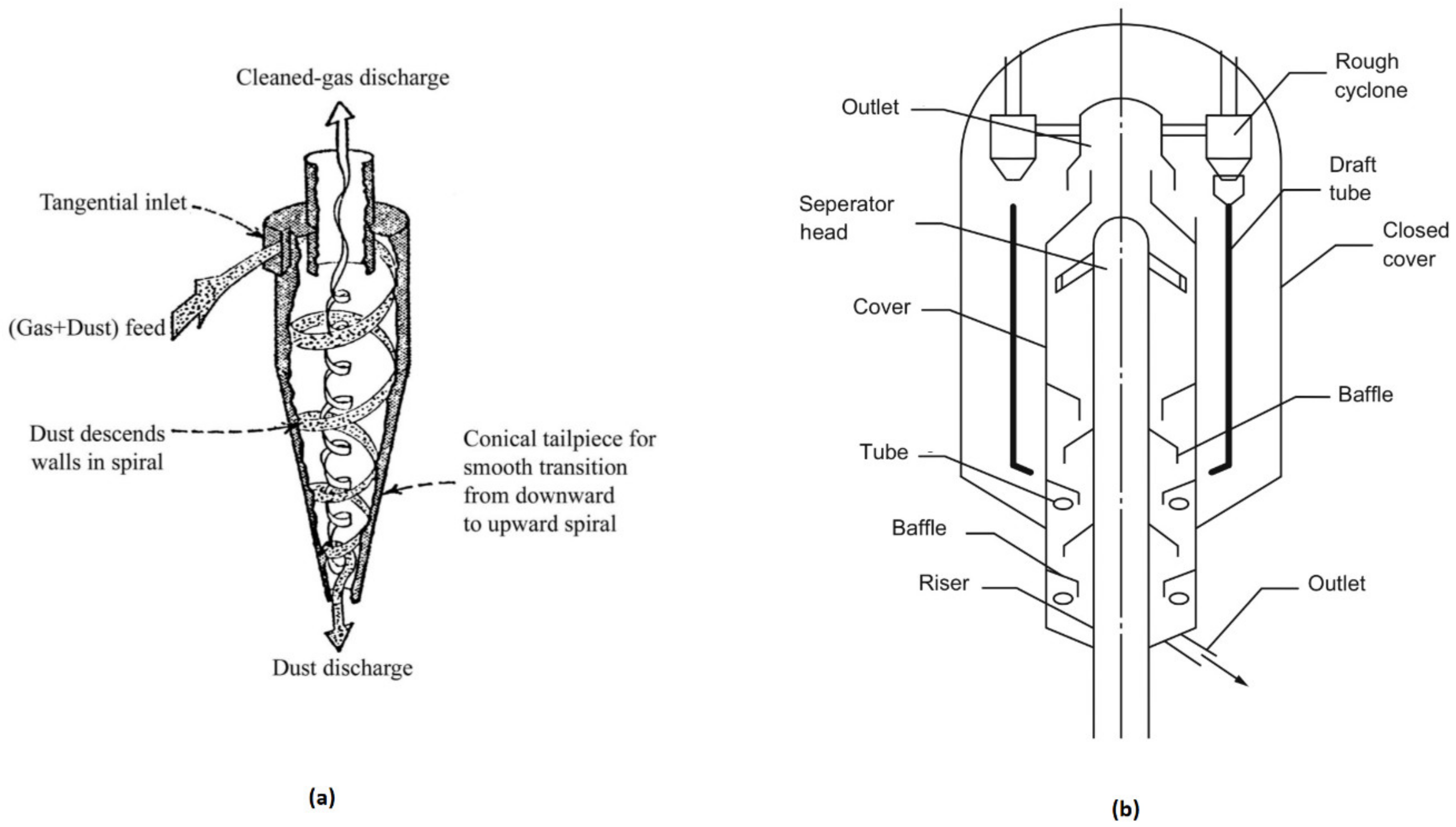
3.1. Cyclones
3.2. Catalyst Transport Lines
4. Conclusions
Author Contributions
Funding
Institutional Review Board Statement
Informed Consent Statement
Acknowledgments
Conflicts of Interest
Nomenclature
| Symbol | Description | Units |
| Molar concentration | ||
| Dispersion coefficient | ||
| Particle diameter | ||
| Smallest particle diameter separated by cyclone | ||
| Mass flow rate | ||
| Acceleration due to gravity | ||
| Height of jet penetration through the bed Enthalpy of the phase | ||
| Deviation coefficient from ideal two-phase flow Reaction rate constant | ||
| Interphase mass transfer coefficient | ||
| Reaction order Molar ratio of hydrogen to Carbon in coke | ||
| Molar flux Number of cyclones | ||
| Number of turns made spirally down a cyclone | ||
| Pressure | ||
| Reaction rate | ||
| Component reaction rate Ideal gas constant | ||
| Reynolds number | ||
| Energy source term | ||
| Temperature | ||
| Bubble rise velocity | ||
| Gas circulation velocity inside rising bubbles | ||
| Minimum bubbling velocity | ||
| Minimum fluidisation velocity | ||
| Terminal velocity of particles in the bed | ||
| Volume | ||
| Mass of holdup in reactor or cyclone | ||
| Mole fraction | ||
| Deviation coefficient from ideal two-phase flow | ||
| Greek letters and other symbols | ||
| Volume fraction | ||
| Exponent of velocity distribution in a cyclone vortex | ||
| Molar ratio of to | ||
| Density | ||
| Ratio of particle radius to radius of the cyclone | ||
| Cyclone separation efficiency | ||
| Cyclone Pressure drop parameter | ||
| Dimensionless tangential velocity at cyclone wall | ||
| Heat of reaction | ||
| Pressure drop | ||
| Enthalpy change of reaction | ||
| Subscripts | ||
| Emulsion | ||
| Bubble phase | ||
| Bubble to emulsion | ||
| Emulsion to bubble | ||
| Carbon monoxide | ||
| Coke | ||
| Carbon dioxide | ||
| Water vapor | ||
| Catalyst | ||
| Gas | ||
References
- Arbel, A.; Huang, Z.; Rinard, I.H.; Shinnar, R.; Sapre, A.V. Dynamic and Control of Fluidized Catalytic Crackers. 1. Modeling of the Current Generation of FCC’s. Ind. Eng. Chem. Res. 1995, 34, 1228–1243. [Google Scholar] [CrossRef]
- Sadeghbeigi, R. Fluid Catalytic Cracking Handbook: An Expert Guide to the Practical Operation, Design, and Optimization of FCC Units; Butterworth-Heinemann: Oxford, UK, 2012. [Google Scholar] [CrossRef]
- Kim, S.W.; Kim, S.D. Void properties in dense bed of cold-flow fluid catalytic cracking regenerator. Processes 2018, 6, 80. [Google Scholar] [CrossRef] [Green Version]
- Wetherald, R.T.; Manabe, S. Sensitivity Studies of Climate Involving Changes in Co2 Concentration. Dev. Atmos. Sci. 1979, 10, 57–64. [Google Scholar] [CrossRef]
- UNFCCC. Paris Agreement. Int. Leg. Mater. 2016, 55, 740–755. [Google Scholar] [CrossRef]
- UNFCCC. National Inventory Submissions 2020|UNFCCC n.d. Available online: https://unfccc.int/ghg-inventories-annex-i-parties/2020 (accessed on 28 June 2021).
- UNFCCC. Kyoto Protocol to the United Nations Framework Convention on Climate Change. Am. J. Int. Law 1998, 92, 315–331. [Google Scholar] [CrossRef]
- Berruti, F.; Pugsley, T.S.; Godfroy, L.; Chaouki, J.; Patience, G.S. Hydrodynamics of circulating fluidized bed risers: A review. Can. J. Chem. Eng. 1995, 73, 579–602. [Google Scholar] [CrossRef]
- Grace, J.R.; Avidan, A.A.; Knowlton, T.M. Circulating Fluidized Beds; Blackie Academic & Professional: London, UK, 1997. [Google Scholar]
- Han, I.S.; Chung, C.B. Dynamic modeling and simulation of a fluidized catalytic cracking process. Part I: Process modeling. Chem. Eng. Sci. 2001, 56, 1951–1971. [Google Scholar] [CrossRef]
- Kunii, D.; Levenspiel, O. Fluidization Engineering; Butterworth-Heinemann: Oxford, UK, 1991. [Google Scholar]
- Shah, M.; Utikar, R.; Pareek, V.; Evans, G.; Joshi, J. Computational fluid dynamic modelling of FCC riser: A review. Chem. Eng. Res. Des. 2016, 1, 403–448. [Google Scholar] [CrossRef]
- Toomey, R.D.; Johnstone, H.F. Gas Fluidization of Solid Particles. Chem. Eng. Prog. Vol. 1952, 48, 220–226. [Google Scholar]
- Kunii, D.; Levenspiel, O. Fluidization Engineering; John Wiley and Sons: New York, NY, USA, 1969. [Google Scholar]
- Kunii, D.; Levenspiel, O. Bubbling bed model: Model for the Flow of Gas through a Fluidized Bed. Ind. Eng. Chem. Fundam. 1968, 7, 446–452. [Google Scholar] [CrossRef]
- Stephens, G.K.; Sinclair, R.J.; Potter, O.E. Gas exchange between bubbles and dense phase in a fluidised bed. Powder Technol. 1967, 1, 157–166. [Google Scholar] [CrossRef]
- Kato, K.; Wen, C.Y. Bubble assemblage model for fluidized bed catalytic reactors. Chem. Eng. Sci. 1969, 24, 1351–1369. [Google Scholar] [CrossRef]
- Han, I.S.; Chung, C.B. Dynamic modeling and simulation of a fluidized catalytic cracking process. Part II: Property estimation and simulation. Chem. Eng. Sci. 2001, 56, 1973–1990. [Google Scholar] [CrossRef]
- Ali, H.; Rohani, S.; Corriou, J.P. Modelling and control of a riser type fluid catalytic cracking (FCC) unit. Chem. Eng. Res. Des. 1997, 75, 401–412. [Google Scholar] [CrossRef]
- Yakubu, J.M.; Patel, R.; Mujtaba, I.M. Optimization of fluidized catalytic cracking unit regenerator to minimize CO2 emissions. Chem. Eng. Trans. 2017, 57, 1531–1536. [Google Scholar] [CrossRef]
- Arthur, J.R. Reactions between Carbon and Oxygen. Trans. Faraday Soc. 1951, 47, 164–178. [Google Scholar] [CrossRef]
- Weisz, P.B. Corn bustion of Carbonaceous Deposits within Porous Catalyst Particles III. The CO2CO Product Ratio. J. Catal. 1966, 6, 425–430. [Google Scholar] [CrossRef]
- Weisz, P.B.; Goodwin, R.B. Combustion of Carbonaceous Deposits within Porous Catalyst Particles II. Intrinsic Burning Rate. J. Catal. 1966, 6, 227–236. [Google Scholar] [CrossRef]
- Weisz, P.B.; Goodwin, I.D. Combustion of Carbonaceous Deposits within Porous Catalyst Particles I. Diffusion-Controlled Kinetics. J. Catal. 1963, 2, 397–404. [Google Scholar] [CrossRef]
- Tone, S.; Miura, S.-I.; Otake, T. Kinetics of Oxidation of Coke on Silica-Alumina Catalysts. Bull. Jpn. Pet. Inst. 1972, 14, 76–82. [Google Scholar] [CrossRef]
- Hano, T.; Nakashio, F.; Kusunoki, K. The burning rate of coke deposited on zeolite catalyst. J. Chem. Eng. Jpn. 1975, 8, 127–130. [Google Scholar] [CrossRef] [Green Version]
- Wang, G.X.; Lin, S.X.; Mo, W.J.; Peng, C.L.; Yang, G.H. Kinetics of Combustion of Carbon and Hydrogen in Carbonaceous Deposits on Zeolite-Type Cracking Catalysts. Ind. Eng. Chem. Process Des. Dev. 1986, 25, 626–630. [Google Scholar] [CrossRef]
- Arandes, J.M.; Abajo, I.; Fernández, I.; López, D.; Bilbao, J. Kinetics of gaseous product formation in the coke combustion of a fluidized catalytic cracking catalyst. Ind. Eng. Chem. Res. 1999, 38, 3255–3260. [Google Scholar] [CrossRef]
- Amblard, B.; Singh, R.; Gbordzoe, E.; Raynal, L. CFD modeling of the coke combustion in an industrial FCC regenerator. Chem. Eng. Sci. 2017, 170, 731–742. [Google Scholar] [CrossRef]
- Hosseini, S.H.; Rahimi, R.; Zivdar, M.; Samimi, A. CFD simulation of gas-solid bubbling fluidized bed containing FCC particles. Korean J. Chem. Eng. 2009, 26, 1405–1413. [Google Scholar] [CrossRef]
- Azarnivand, A.; Behjat, Y.; Safekordi, A.A. CFD simulation of gas-solid flow patterns in a downscaled combustor-style FCC regenerator. Particuology 2018, 39, 96–108. [Google Scholar] [CrossRef]
- Lee, L.S.; Yu, S.W.; Cheng, C.T.; Pan, W.Y. Fluidized-bed catalyst cracking regenerator modelling and analysis. Chem. Eng. J. 1989, 40, 71–82. [Google Scholar] [CrossRef]
- Qian, K.; Tomczak, D.C.; Rakiewicz, E.F.; Harding, R.H.; Yaluris, G.; Cheng, W.C.; Zhao, X.; Peters, A.W. Coke formation in the fluid catalytic cracking process by combined analytical techniques. Energy Fuels 1997, 11, 596–600. [Google Scholar] [CrossRef]
- Luan, H.; Lin, J.; Xiu, G.; Ju, F.; Ling, H. Study on compositions of FCC flue gas and pollutant precursors from FCC catalysts. Chemosphere 2020, 245, 125528. [Google Scholar] [CrossRef]
- Ibarra, Á.; Veloso, A.; Bilbao, J.; Arandes, J.M.; Castaño, P. Dual coke deactivation pathways during the catalytic cracking of raw bio-oil and vacuum gasoil in FCC conditions. Appl. Catal. B Environ. 2016, 182, 336–346. [Google Scholar] [CrossRef] [Green Version]
- Elshishini, S.S.; Elnashaie, S.S.E.H. Digital simulation of industrial fluid catalytic cracking units: Bifurcation and its implications. Chem. Eng. Sci. 1990, 45, 553–559. [Google Scholar] [CrossRef]
- Bai, D.; Zhu, J.X.; Jin, Y.; Yu, Z. Simulation of FCC catalyst regeneration in a riser regenerator. Chem. Eng. J. 1998, 71, 97–109. [Google Scholar] [CrossRef]
- Bayraktar, O.; Kugler, E.L. Coke content of spent commercial fluid catalytic cracking (FCC) catalysts: Determination by temperature-programmed oxidation. J. Therm. Anal. Calorim. 2003, 71, 867–874. [Google Scholar] [CrossRef] [Green Version]
- Hashimoto, K.; Takatani, K.; Iwasa, H.; Masuda, T. A multiple-reaction model for burning regeneration of coked catalysts. Chem. Eng. J. 1983, 27, 177–186. [Google Scholar] [CrossRef]
- Dimitriadis, V.D.; Lappas, A.A.; Vasalos, I.A. Kinetics of combustion of carbon in carbonaceous deposits on zeolite catalysts for fluid catalytic cracking units (FCCU). Comparison between Pt and non Pt-containing catalysts. Fuel 1998, 77, 1377–1383. [Google Scholar] [CrossRef]
- Morley, K.; De, L. On the Determination of Regeneration of Kinetic Parameters for the Craclung Catalyst. Can. J. Chem. Eng. 1987, 65, 773–777. [Google Scholar] [CrossRef]
- Howard, J.B.; Williams, G.C.; Fine, D.H. Kinetics of Carbon Monoxide Oxidation in Postflame Gases. In Symposium (International) on Combustion; Elsevier: Amsterdam, The Netherlands, 1973. [Google Scholar]
- Li, C.; Brown, T.C. Carbon oxidation kinetics from evolved carbon oxide analysis during temperature-programmed oxidation. Carbon 2001, 39, 725–732. [Google Scholar] [CrossRef]
- Kanervo, J.M.; Krause, A.O.I.; Aittamaa, J.R.; Hagelberg, P.H.; Lipiäinen, K.J.T.; Eilos, I.H.; Hiltunen, J.S.; Niemi, V.M. Kinetics of the regeneration of a cracking catalyst derived from TPO measurements. Chem. Eng. Sci. 2001, 56, 1221–1227. [Google Scholar] [CrossRef]
- Williams, G.C.; Hottel, H.C.; Morgan, A.C. The Combustion of Methane in a Jet-Mixed Reactor. In Symposium (International) on Combustion; Elsevier: Amsterdam, The Netherlands, 1969; Volume 12, pp. 913–925. [Google Scholar] [CrossRef]
- Schneider, G.R. Kinetics of Propane Combustion in a Well Stirred Reactor. Ph.D. Thesis, Massachusetts Institute of Technology, Department of Nuclear Engineering, Cambridge, MA, USA, 1961. [Google Scholar]
- Friedman, R.; Cyphers, J.A. Flame structure studies. III. Gas sampling in a low-pressure propane-air flame. J. Chem. Phys. 1955, 23, 1875–1880. [Google Scholar] [CrossRef]
- Singh, T.; Sawyer, R.F. CO Reactions in the Afterflame Region of Ethylene/Oxygen and Ethane/Oxygen Flames. In Symposium (International) on Combustion; Elsevier: Amsterdam, The Netherlands, 1971; Volume 13, pp. 403–416. [Google Scholar] [CrossRef]
- Sobolev, G.K. High-Temperature Oxidation and Burning of Carbon Monoxide. In Symposium (International) on Combustion; Elsevier: Amsterdam, The Netherlands, 1958; Volume 7, pp. 386–391. [Google Scholar] [CrossRef]
- Ghazal, F.P.H. Kinetics of Carbon Monoxide Oxidation in Combustion Products. Ph.D. Thesis, Massachusetts Institute of Technology, Cambridge, MA, USA, 1971. [Google Scholar]
- Morley, K.; de Lasa, H.I. Regeneration of cracking catalyst influence of the homogeneous CO postcombustion reaction. Can. J. Chem. Eng. 1988, 66, 428–432. [Google Scholar] [CrossRef]
- Ahmed, S.; Back, M.H. The role of the surface complex in the kinetics of the reaction of oxygen with carbon. Carbon 1985, 23, 513–524. [Google Scholar] [CrossRef]
- Tucker, B.G.; Mulcahy, M.F.R. Formation and decomposition of surface oxide in carbon combustion. Trans. Faraday Soc. 1969, 65, 274–286. [Google Scholar] [CrossRef]
- Geldart, D. Types of gas fluidization. Powder Technol. 1973, 7, 285–292. [Google Scholar] [CrossRef]
- Baeyens, J.; Geldart, D. Predictive Calculations of Flow Parameters in Gas Fluidized Beds and Fluidization Behaviour of Various Powders. In Proceedings the International Symposium Fluidization and Its Applications; Cepadues Edition: Toulouse, France, 1973; p. 263. [Google Scholar]
- Yates, J.G. Fundamentals of Fluidized-Bed Chemical Processes: Butterworths Monographs in Chemical Engineering; Butterworth-Heinemann: Oxford, UK, 1983. [Google Scholar]
- Kumar, A.; sen Gupta, P. Prediction of minimum fluidization velocity for multicomponent mixtures. Indian J. Technol. 1974, 12, 225–227. [Google Scholar]
- Mawatari, Y.; Tatemoto, Y.; Noda, K. Prediction of minimum fluidization velocity for vibrated fluidized bed. Powder Technol. 2003, 131, 66–70. [Google Scholar] [CrossRef]
- Rowe, P.N.; Nienow, A.W. Minimum fluidisation velocity of multi-component particle mixtures. Chem. Eng. Sci. 1975, 30, 1365–1369. [Google Scholar] [CrossRef]
- Asif, M. Predicting minimum fluidization velocities of multi-component solid mixtures. Particuology 2013, 11, 309–316. [Google Scholar] [CrossRef]
- Delebarre, A. Revisiting the Wen and Yu equations for minimum fluidization velocity prediction. Chem. Eng. Res. Des. 2004, 82, 587–590. [Google Scholar] [CrossRef]
- Amarasinghe, W.S.; Jayarathna, C.K.; Ahangama, B.S.; Tokheim, L.A.; Moldestad, B.M.E. Experimental Study and CFD Modelling of Minimum Fluidization Velocity for Geldart A, B and D Particles. Int. J. Model. Optim. 2017, 7, 152–156. [Google Scholar] [CrossRef] [Green Version]
- Zhang, X.; Zhou, Y.; Zhu, J. Enhanced fluidization of group A particles modulated by group C powder. Powder Technol. 2021, 377, 684–692. [Google Scholar] [CrossRef]
- Lee, J.R.; Lee, K.S.; Hasolli, N.; Park, Y.O.; Lee, K.Y.; Kim, Y.H. Fluidization and mixing behaviors of Geldart groups A, B and C particles assisted by vertical vibration in fluidized bed. Chem. Eng. Process. Process Intensif. 2020, 149, 107856. [Google Scholar] [CrossRef]
- Frank, D.J.; Roland, C.; David, H. Fluidization, 2nd ed.; Academic Press Inc.: Cambridge, MA, USA, 1985. [Google Scholar]
- Anantharaman, A.; Cocco, R.A.; Chew, J.W. Evaluation of correlations for minimum fluidization velocity (Umf) in gas-solid fluidization. Powder Technol. 2018, 323, 454–485. [Google Scholar] [CrossRef]
- Shaul, S.; Rabinovich, E.; Kalman, H. Generalized flow regime diagram of fluidized beds based on the height to bed diameter ratio. Powder Technol. 2012, 228, 264–271. [Google Scholar] [CrossRef]
- Shaul, S.; Rabinovich, E.; Kalman, H. Typical fluidization characteristics for Geldart’s classification groups. Part. Sci. Technol. 2014, 32, 197–205. [Google Scholar] [CrossRef]
- Kong, W.; Tan, T.; Baeyens, J.; Flamant, G.; Zhang, H. Bubbling and Slugging of Geldart Group A Powders in Small Diameter Columns. Ind. Eng. Chem. Res. 2017, 56, 4136–4144. [Google Scholar] [CrossRef]
- Abrahamsen, A.R.; Geldart, D. Behaviour of gas-fluidized beds of fine powders part I. Homogeneous expansion. Powder Technol. 1980, 26, 35–46. [Google Scholar] [CrossRef]
- Rowe, P.N.; Yacono, C.X.R. The bubbling behaviour of fine powders when fluidised. Chem. Eng. Sci. 1976, 31, 1179–1192. [Google Scholar] [CrossRef]
- Rowe, P.N.; Partridge, B.A. X-ray study of bubbles in fluidized beds. Process Saf. Environ. Prot. Trans. Inst. Chem. Eng. Part B 1965, 43, 157–175. [Google Scholar]
- Rowe, P.N.; Partridge, B.A. An X-ray study of bubbles in fluidised beds. Chem. Eng. Res. Des. 1997, 75, S116–S134. [Google Scholar] [CrossRef]
- Rowe, P.N.; Everett, D.J. Fluidised bed bubbles viewed by X-rays. Part I: Experimental details and the interaction of bubbles with solid surfaces. Trans. Inst. Chem. Eng. 1972, 50, 42–48. [Google Scholar]
- Yacono, C.X.R. An X-Ray Study of Bubbles in Gas-Fluidised Beds of Small Particles. Ph.D. Thesis, University College London, London, UK, 1975. [Google Scholar]
- Rowe, P.N. A note on the motion of a bubble rising through a fluidized bed. Chem. Eng. Sci. 1964, 19, 75–77. [Google Scholar] [CrossRef]
- Rowe, P.N. Prediction of bubble size in a gas fluidised bed. Chem. Eng. Sci. 1976, 31, 285–288. [Google Scholar] [CrossRef]
- Yang, W. Handbook of Fluidization and Fluid-Particle Systems; CRC Press: New York, NY, USA, 2003. [Google Scholar]
- Whitehead, A.B.; Gartside, G.; Dent, D.C. Fluidization studies in large gas-solid systems. Part III. The effect of bed depth and fluidizing velocity on solids circulation patterns. Powder Technol. 1976, 14, 61–70. [Google Scholar] [CrossRef]
- Geldart, D. The size and frequency of bubbles in two- and three-dimensional gas-fluidised beds. Powder Technol. 1970, 4, 41–55. [Google Scholar] [CrossRef]
- Werther, J. Bubble growth in large diameter fluidized beds. Fluid Technol. 1975, 1, 215. [Google Scholar]
- Mori, S.; Wen, C.Y. Estimation of bubble diameter in gaseous fluidized beds. AIChE J. 1975, 21, 109–115. [Google Scholar] [CrossRef]
- Cai, P.; Schiavetti, M.; de Michele, G.; Grazzini, G.C.; Miccio, M. Quantitative estimation of bubble size in PFBC. Powder Technol. 1994, 80, 99–109. [Google Scholar] [CrossRef]
- Darton, R.C.; Nauze, R.; Harrison, D.; Davidson, J. Bubble Growth due to Coalescence in Fluidised Beds. In Chemical Reactor Theory; Lapidus, I., Amundson, N.R., Eds.; Prentice-Hall: New York, NY, USA, 1977. [Google Scholar]
- Horio, M.; Nonaka, A. A generalized bubble diameter correlation for gas-solid fluidized beds. AIChE J. 1987, 33, 1865–1872. [Google Scholar] [CrossRef]
- Rowe, P.N. Experimental Properties of Bubbles. Fluidization; Academic Press: New York, NY, USA, 1971; p. 121. [Google Scholar]
- Harrison, D.; Davidson, J.F.; de Kock, J.W. Bubble growth theory in fluidized beds. Chem. Eng. Sci. 1961, 39, 202. [Google Scholar]
- Davidson, J.F.; Harrison, D. Fluidized Particles; Cambridge University Press: Cambridge, NY, USA, 1963. [Google Scholar]
- Upson, P.C.; Pyle, D.L. The Stability of Bubbles in Fluidized Beds. In Fluidization and its Applications: Proceedings of the International Symposium; Cepadues Edition: Toulouse, France, 1973; pp. 207–222. [Google Scholar]
- Clift, R.; Grace, J.R.; Weber, M.E. Stability of Bubbles in Fluidized Beds. Ind. Eng. Chem. Fundam. 1974, 13, 45–51. [Google Scholar] [CrossRef]
- Rice, W.J.; Wilhelm, R.H. Surface dynamics of fluidized beds and quality of fluidization. AIChE J. 1958, 4, 423–429. [Google Scholar] [CrossRef]
- Karimipour, S.; Pugsley, T. A critical evaluation of literature correlations for predicting bubble size and velocity in gas–solid fluidized beds. Powder Technol. 2011, 205, 1–14. [Google Scholar] [CrossRef]
- Davies, R.M.; Taylor, G.I. The mechanics of large bubbles rising through extended liquids and through liquids in tubes. Proc. R. Soc. Lond. Ser. A Math. Phys. Sci. 1950, 200, 375–390. [Google Scholar] [CrossRef]
- Sit, S.P.; Grace, J.R. Effect of bubble interaction on interphase mass transfer in gas fluidized beds. Chem. Eng. Sci. 1981, 36, 327–335. [Google Scholar] [CrossRef]
- Chiba, T.; Kobayashi, H. Solid exchange between the bubble wake and the emulsion phase in a gas-fluidised bed. J. Chem. Eng. Jpn. 1977, 10, 206–210. [Google Scholar] [CrossRef] [Green Version]
- Pyle, D.L.; Harrison, D. An experimental investigation of the two-phase theory of fluidization. Chem. Eng. Sci. 1967, 22, 1199–1207. [Google Scholar] [CrossRef]
- Pyle, D.L.; Harrison, D. The rising velocity of bubbles in two-dimensional fluidised beds. Chem. Eng. Sci. 1967, 22, 531–535. [Google Scholar] [CrossRef]
- Marsheck, R.M.; Gomezplata, A. Particle flow patterns in a fluidized bed. AIChE J. 1965, 11, 167–173. [Google Scholar] [CrossRef]
- Gabor, J.D. On the mechanics of fluidized particle movement. Chem. Eng. J. 1972, 4, 118–126. [Google Scholar] [CrossRef]
- Stein, M.; Ding, Y.L.; Seville, J.P.K.; Parker, D.J. Solids motion in bubbling gas fluidized beds. Chem. Eng. Sci. 2000, 55, 5291–5300. [Google Scholar] [CrossRef]
- Mostoufi, N.; Chaouki, J. Local solid mixing in gas–solid fluidized beds. Powder Technol. 2001, 114, 23–31. [Google Scholar] [CrossRef]
- Shabanian, J.; Chaouki, J. Influence of interparticle forces on solids motion in a bubbling gas-solid fluidized bed. Powder Technol. 2016, 299, 98–106. [Google Scholar] [CrossRef]
- Werther, J.; Molerus, O. The local structure of gas fluidized beds -II. The spatial distribution of bubbles. Int. J. Multiph. Flow 1973, 1, 123–138. [Google Scholar] [CrossRef]
- Callcott, T.G.; Rigby, G.R.; Singh, B. Experiences in the handling of particulate materials. BHP Tech. Bull. 1975, 19, 20. [Google Scholar]
- Gabor, J.D. Lateral solids mixing in fludized-packed beds. AIChE J. 1964, 10, 345–350. [Google Scholar] [CrossRef]
- Hirama, T.; Ishida, M.; Shirai, T. The Lateral Dispersion of Solid Particles in Fluidized Beds. Kagaku Kogaku Ronbunshu 1975, 1, 272–276. [Google Scholar] [CrossRef]
- Mori, Y.; Nakamura, K. Solid Mixing in Fluidised Bed. Chem. Eng. 1965, 29, 868–875. [Google Scholar] [CrossRef] [Green Version]
- Fan, L.T.; Shl, Y.F. Lateral Mixing of Solids in Batch Gas-Solids Fluidized Beds. Ind. Eng. Chem. Process Des. Dev. 1984, 23, 337–341. [Google Scholar] [CrossRef]
- Merry, J. Gulf stream circulation in shallow fluidized beds. Trans. Inst. Chem. Eng. 1973, 51, 361–368. [Google Scholar]
- Grace, J.R. Processes. In AIChE Symposium Series; McGill Univ.: Montreal, QC, Canada, 1974. [Google Scholar]
- Harris, B.J. Modeling options for circulating fluidized beds: A core/annulus deposition model. Circ. Fluid. Bed Technol. 1994, 32–39. [Google Scholar]
- Grace, J.R.; Clift, R. On the two-phase theory of fluidization. Chem. Eng. Sci. 1974, 29, 327–334. [Google Scholar] [CrossRef]
- Rowe, P.N. A model for chemical reaction in the entry region of a gas fluidised-bed reactor. Chem. Eng. Sci. 1993, 48, 2519–2524. [Google Scholar] [CrossRef]
- Sane, S.U.; Haynes, H.W.; Agarwal, P.K. An experimental and modelling investigation of gas mixing in bubbling fluidized beds. Chem. Eng. Sci. 1996, 51, 1133–1147. [Google Scholar] [CrossRef]
- Rowe, P.N. Two-Phase Theory and Fluidized Bed Reactor Models; ACS Symposium Series; ACS: Houston, TX, USA, 1978; Volume 65, pp. 436–446. [Google Scholar] [CrossRef]
- Darton, R. A Bubble growth theory of fluidised bed reactors. Trans. Inst. Chem. Eng. 1979, 57, 134–138. [Google Scholar]
- Behie, L.A.; Kehoe, P. The grid region in a fluidized bed reactor. AIChE J. 1973, 19, 1070–1072. [Google Scholar] [CrossRef]
- Markhevka, V.I.; Basov, V.A.; Melik-Akhnazarov, T.K.; Orochko, D.I. The flow of a gas jet into a fluidized bed. Theor. Found. Chem. Eng. 1971, 5, 80. [Google Scholar]
- Kececioglu, I.; Yang, W.-C.; Keairns, D.L. Fate of solids fed pneumatically through a jet into a fluidized bed. AIChE J. 1984, 30, 99–110. [Google Scholar] [CrossRef]
- Rowe, P.N.; MacGillivray, H.J.; Cheesman, D. Gas discharge from an orifice into a gas fluidised bed. Trans. Inst. Chem. Eng. 1979, 57, 194–199. [Google Scholar]
- Kozin, V.E.; Baskakov, A.P. A study of the grating region of fluidized bed above bubble-cap-type gas-distributors. Chem. Technol. Fuels Oils 1967, 3, 544–547. [Google Scholar] [CrossRef]
- Baerns, M.; Fetting, F. Quenching of a Hot Gas Stream in a Gas Fluidized Bed. Chem. Eng. Sci. 1964, 20, 273–280. [Google Scholar] [CrossRef]
- Merry, J.M.D. Fluid and particle entrainment into vertical jets in fluidized beds. AIChE J. 1976, 22, 315–323. [Google Scholar] [CrossRef]
- Merry, J.M.D. Penetration of vertical jets into fluidized beds. AIChE J. 1975, 21, 507–510. [Google Scholar] [CrossRef]
- Kunii, D.; Levenspiel, O.; Levenspiel, O. Fluidized Reactor Models. 1. For Bubbling Beds of Fine, Intermediate, and Large Particles. 2. For the Lean Phase: Freeboard and Fast Fluidization. Ind. Eng. Chem. Res. 1990, 29, 1226–1234. [Google Scholar] [CrossRef]
- Levenspiel, O.; Kunii, D.; Fitzgerald, T. The processing of solids of changing size in bubbling fluidized beds. Powder Technol. 1968, 2, 87–96. [Google Scholar] [CrossRef]
- Cooke, M.J.; Harris, W.; Highley, J.; Williams, D.F. Kinetics of oxygen consumption in fluidized bed carbonizers. Tripart. Chem. Eng. Conf. Symp. Fluid. I 1968, 30, 14–20. [Google Scholar]
- Kumar, S.; Chadha, A.; Gupta, R.; Sharma, R. CATCRAK: A Process Simulator for an Integrated FCC-Regenerator System. Ind. Eng. Chem. Res. 1995, 34, 3737–3748. [Google Scholar] [CrossRef]
- de Lasa, H.I.; Errazu, A.; Barreiro, E.; Solioz, S. Analysis of fluidized bed catalytic cracking regenerator models in an industrial scale unit. Can. J. Chem. Eng. 1981, 59, 549–553. [Google Scholar] [CrossRef]
- Errazu, A.F.; de Lasa, H.I.; Sarti, F. Fluidized bed catalytic cracking regenerator model: Grid effects. Can. J. Chem. Eng. 1979, 57, 2. [Google Scholar]
- Filho, R.M.; Batista, L.M.F.L.; Fusco, M. A fast fluidized bed reactor for industrial FCC regenerator. Chem. Eng. Sci. 1996, 51, 1807–1816. [Google Scholar] [CrossRef]
- Faltsi-Saravelou, O.; Vasalos, I.A.; Dimogiorgas, G. FBSim: A model for fluidized bed simulation-II. Simulation of an industrial fluidized catalytic cracking regenerator. Comput. Chem. Eng. 1991, 15, 647–656. [Google Scholar] [CrossRef]
- Krishna, A.S.; Parkin, E.S. Modeling the regenerator in commercial fluid catalytic cracking units. Chem. Eng. Prog. 1985, 81, 55–62. [Google Scholar]
- Penteado, J.C.; Rossi, L.F.; Negrão, C.O. Numerical Modelling of a FCC Regenerator. In Proceedings of the 17th International Congress of Mechanical Engineering (COBEM), Sao Paulo, Brazil, 10–14 November 2003. [Google Scholar]
- Fernandes, J.L.; Verstraete, J.J.; Pinheiro, C.I.C.; Oliveira, N.M.C.; Ramôa Ribeiro, F. Dynamic modelling of an industrial R2R FCC unit. Chem. Eng. Sci. 2007, 62, 1184–1198. [Google Scholar] [CrossRef]
- Daly, C.; Tidjani, N.; Martin, G.; Roesler, J. Détermination des Paramétres Cinétiques dans la Régénération des Catalyseurs de FCC; Technical Report No. 56010; Institut Français du Pétrole (IFP): Paris, France, 2001. [Google Scholar]
- Zwinkels, M. FCC Regenerator Simulation Model. Ph.D. Thesis, Institute Francais du Pétrole (IFP), Paris, France, 1997. [Google Scholar]
- Shaikh, A.A.; Al-Mutairi, E.M.; Ino, T. Modeling and simulation of a downer-type HS-FCC unit. Ind. Eng. Chem. Res. 2008, 47, 9018–9024. [Google Scholar] [CrossRef]
- Dasila, P.K.; Choudhury, I.; Saraf, D.; Chopra, S.; Dalai, A. Parametric Sensitivity Studies in a Commercial FCC Unit. Adv. Chem. Eng. Sci. 2012, 2, 136–149. [Google Scholar] [CrossRef] [Green Version]
- Kim, S.; Urm, J.; Kim, D.S.; Lee, K.; Lee, J.M. Modeling, simulation and structural analysis of a fluid catalytic cracking (FCC) process. Korean J. Chem. Eng. 2018, 35, 2327–2335. [Google Scholar] [CrossRef]
- Grace, J.R. Fluidized Bed Reactor Modeling; ACS Symposium Series; ACS: Washington, DC, USA, 1981; Volume 22, pp. 3–18. [Google Scholar] [CrossRef]
- Levenspiel, O. Difficulties in trying to model and scale-up the Bubbling Fluidized Bed (BFB) reactor. Ind. Eng. Chem. Res. 2008, 47, 273–277. [Google Scholar] [CrossRef]
- Faltsi-Saravelou, O.; Vasalos, I.A. FBSim: A model for fluidized bed simulation-I. Dynamic modeling of an adiabatic reacting system of small gas fluidized particles. Comput. Chem. Eng. 1991, 15, 639–646. [Google Scholar] [CrossRef]
- Singh, R.; Gbordzoe, E. Modeling FCC spent catalyst regeneration with computational fluid dynamics. Powder Technol. 2017, 316, 560–568. [Google Scholar] [CrossRef]
- de Lasa, H.I.; Grace, J.R. The influence of the freeboard region in a fluidized bed catalytic cracking regenerator. AIChE J. 1979, 25, 984–991. [Google Scholar] [CrossRef]
- Cao, B.; Zhang, P.; Zheng, X.; Xu, C.; Gao, J. Numerical simulation of hydrodynamics and coke combustions in FCC regenerator. Pet. Sci. Technol. 2008, 26, 256–269. [Google Scholar] [CrossRef]
- Wu, C.; Cheng, Y.; Ding, Y.; Jin, Y. CFD-DEM simulation of gas-solid reacting flows in fluid catalytic cracking (FCC) process. Chem. Eng. Sci. 2010, 65, 542–549. [Google Scholar] [CrossRef]
- Latham, R.; Potter, O.E. Back-mixing of gas in a 6-in diameter fluidised bed. Chem. Eng. J. 1970, 1, 152–162. [Google Scholar] [CrossRef]
- Rowe, P.N.; Partridge, B.A.; Cheney, A.G.; Henwood, G.A.; Lyall, E. Mechanisms of solids mixing in fluidised beds. Trans. Inst. Chem. Eng. Chem. Eng. 1965, 43, T271. [Google Scholar]
- Liu, D.; Chen, X. Lateral solids dispersion coefficient in large-scale fluidized beds. Combust. Flame 2010, 157, 2116–2124. [Google Scholar] [CrossRef]
- Olsson, J.; Pallarès, D.; Johnsson, F. Lateral fuel dispersion in a large-scale bubbling fluidized bed. Chem. Eng. Sci. 2012, 74, 148–159. [Google Scholar] [CrossRef]
- Fan, L.T.; Song, J.C.; Yutani, N. Radial particle mixing in gas-solids fluidized beds. Chem. Eng. Sci. 1986, 41, 117–122. [Google Scholar] [CrossRef]
- IPCC. Climate Change and Land an IPCC Special Report on Climate Change, Desertification, Land Degradation, Sustainable Land Management, Food Security, and Greenhouse Gas Fluxes in Terrestrial Ecosystems; IPCC: Geneva, Switzerland, 2019. [Google Scholar]
- le Quéré, C.; Andrew, R.M.; Friedlingstein, P.; Sitch, S.; Hauck, J.; Pongratz, J.; Pickers, P.A.; Korsbakken, J.; Peters, G.P.; Canadell, J.G.; et al. Global Carbon Budget 2018. Earth Syst. Sci. Data 2018, 10, 2141–2194. [Google Scholar] [CrossRef] [Green Version]
- Scala, F. Fluidized Bed Technologies for Near-Zero Emission Combustion and Gasification; Woodhead Publishing Limited: Cambridge, UK, 2013. [Google Scholar]
- Nakhaei, M.; Lu, B.; Tian, Y.; Wang, W.; Dam-Johansen, K.; Wu, H. CFD Modeling of Gas–Solid Cyclone Separators at Ambient and Elevated Temperatures. Processes 2020, 8, 228. [Google Scholar] [CrossRef] [Green Version]
- Wang, B.; Xu, D.L.; Chu, K.W.; Yu, A.B. Numerical study of gas–solid flow in a cyclone separator. Appl. Math. Model. 2006, 30, 1326–1342. [Google Scholar] [CrossRef] [Green Version]
- Hashemi Shahraki, B. The Development and Validation of New Equations for Prediction of the Performance of Tangential Cyclones. Int. J. Eng. 2003, 16, 109–124. [Google Scholar]
- Lu, C.-X. FCC riser quick separation system: A review. Pet. Sci. 2016, 13, 776–781. [Google Scholar] [CrossRef] [Green Version]
- Wei, Q.; Sun, G.; Yang, J. A model for prediction of maximum-efficiency inlet velocity in a gas-solid cyclone separator. Chem. Eng. Sci. 2019, 204, 287–297. [Google Scholar] [CrossRef]
- Chu, K.W.; Wang, B.; Xu, D.L.; Chen, Y.X.; Yu, A.B. CFD–DEM simulation of the gas–solid flow in a cyclone separator. Chem. Eng. Sci. 2011, 66, 834–847. [Google Scholar] [CrossRef]
- Masnadi, M.S.; Grace, J.R.; Elyasi, S.; Bi, X. Distribution of multi-phase gas–solid flow across identical parallel cyclones: Modeling and experimental study. Sep. Purif. Technol. 2010, 72, 48–55. [Google Scholar] [CrossRef]
- Zhang, R.; Basu, P. A simple model for prediction of solid collection efficiency of a gas–solid separator. Powder Technol. 2004, 147, 86–93. [Google Scholar] [CrossRef]
- Jiang, Y.; Qiu, G.; Wang, H. Modelling and experimental investigation of the full-loop gas–solid flow in a circulating fluidized bed with six cyclone separators. Chem. Eng. Sci. 2014, 109, 85–97. [Google Scholar] [CrossRef]
- Baltrrnas, P.; Vaitiekūnas, P.; Jakštonienn, I.; Konoverskytt, S. Study of gas-solid flow in a multichannel cyclone. J. Environ. Eng. Landsc. Manag. 2012, 20, 129–137. [Google Scholar] [CrossRef]
- Su, Y.; Mao, Y. Experimental study on the gas–solid suspension flow in a square cyclone separator. Chem. Eng. J. 2006, 121, 51–58. [Google Scholar] [CrossRef]
- Lapple, C.E. Gravity and Centrifugal Separation. Am. Ind. Hyg. Assoc. Q. 1950, 11, 40–48. [Google Scholar] [CrossRef]
- Gimbun, J.; Chuah, T.G.; Choong, T.S.Y.; Fakhru’l-Razi, A. A CFD Study on the Prediction of Cyclone Collection Efficiency. Int. J. Comput. Methods Eng. Sci. Mech. 2006, 6, 161–168. [Google Scholar] [CrossRef]
- Dirgo, J.; Leith, D. Aerosol Science and Technology Cyclone Collection Efficiency: Comparison of Experimental Results with Theoretical Predictions. Exp. Results Theor. Predict. Aerosol Sci. Technol. 2007, 4, 401–415. [Google Scholar] [CrossRef] [Green Version]
- Cortés, C.; Gil, A. Modeling the gas and particle flow inside cyclone separators. Prog. Energy Combust. Sci. 2007, 33, 409–452. [Google Scholar] [CrossRef]
- Morin, M.; Raynal, L.; Karri, S.B.R.; Cocco, R. Effect of solid loading and inlet aspect ratio on cyclone efficiency and pressure drop: Experimental study and CFD simulations. Powder Technol. 2021, 377, 174–185. [Google Scholar] [CrossRef]
- Rosin, P.; Rammler, E.; Intelmann, W. Principles and limits of cyclone dust removal. Zeit Ver Dtsch. Ing. 1932, 76, 433–437. [Google Scholar]
- Maheshwari, F.; Parmar, A. A Review Study on Gas-Solid Cyclone Separator using Lapple Model. J. Res. 2018, 4, 1–5. [Google Scholar]
- Hoffmann, A.C.; Stein, L.E. Computational Fluid Dynamics. Gas Cyclones and Swirl Tubes, Berlin, Heidelberg; Springer: Berlin/Heidelberg, Germany, 2002; pp. 123–135. [Google Scholar] [CrossRef] [Green Version]
- Chen, J.; Shi, M. A universal model to calculate cyclone pressure drop. Powder Technol. 2007, 171, 184–191. [Google Scholar] [CrossRef]
- Knowlton, T.; Karri, R.S.B. Differences in cyclone operation at low and high solids loading. In Proceedings of the International Fluidization South Africa Conference, Johannesburg, South Africa, 19–20 November 2008; pp. 119–160. [Google Scholar]
- Li, S.; Yang, H.; Wu, Y.; Zhang, H. Improved cyclone pressure drop model at high inlet solid concentrations. Chem. Eng. Technol. 2011, 34, 1507–1513. [Google Scholar] [CrossRef]
- Casal, J.; Martinez-Benet, J.M. A better way to calculate cyclone pressure drop. Chem. Eng. 1983, 90, 99–100. [Google Scholar]


| Regenerator | Dimensions | |
|---|---|---|
 | Height | |
| Diameter | ||
| Operating Conditions | ||
| Gas oil inlet T | ||
| Catalyst inlet T | ||
| Catalyst exit T | ||
| Coke entering | ||
| Coke leaving | ||
| Pressure | ||
| Solid Residence | ||
| Model Classification | Description | Governing Mass Balance Equations |
|---|---|---|
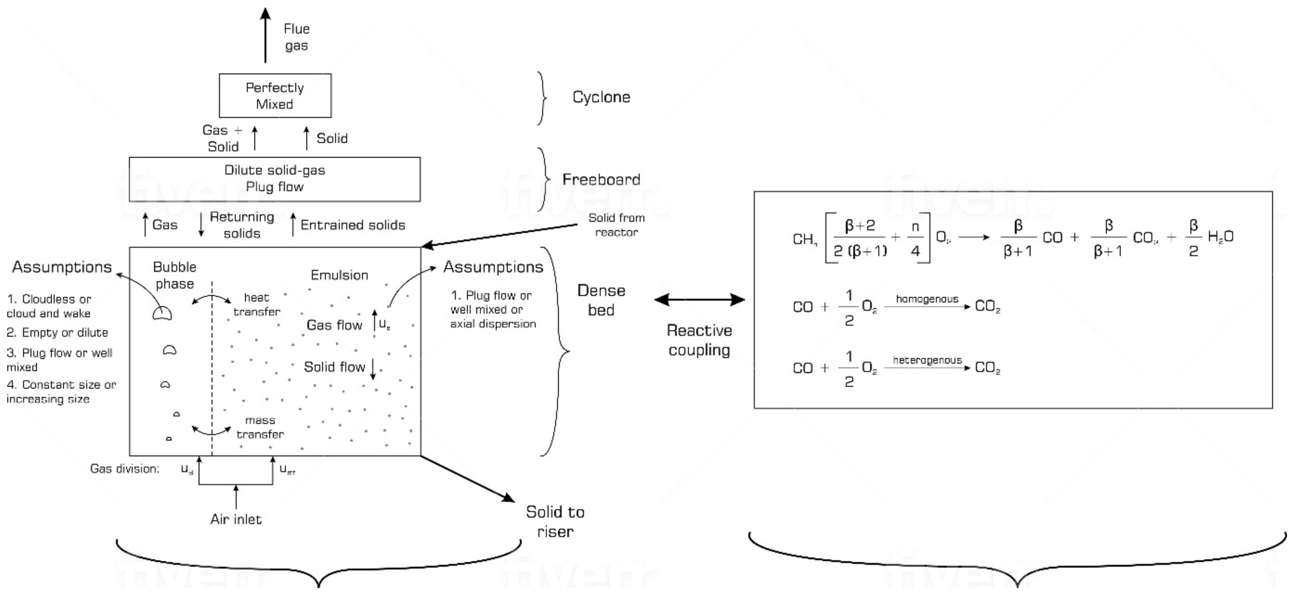
Two-Phase Flow Models | This model was first proposed by Toomey and Johnstone [13]. It draws from the observations of bubbles rising in bubbling beds and postulates that two phases in the bed exist, i.e., the emulsion and the bubble phase. According to the original theory from Toomey and Johnstone, the emulsion phase is at minimum fluidisation conditions while any gas through the distributor plate in excess of that required for incipient fluidisation passes through the bed in the form of bubbles (i.e., the bubble phase). Each phase is represented by a mass balance equation, and an interchange term is included in each equation for transfer between the phases. If more than one component is present in the phase, i.e., a mixture of gas in air bubbles, separate equations are written for each phase. Generally, gas flow in the bubbles is assumed to be plug flow, while gas flow in the emulsion is assumed plug flow or well-mixed [78]. However, non-ideality of flow in dense beds is likely, so models can replace traditional ideal flow with dispersion models, tanks in series and residence time distribution models. | For emulsion gas: For bubble phase: ; For plug flow and for well-mixed flow for dispersion model is defined. |
Bubbling bed Models or Cloud and Wake Models | These models are an extension of the two-phase models. They were first proposed by Kunii and Levenspiel [15,125,126] to account for the cloud and wake regions that were seen from X-ray imagining studies [72,73]. This consideration of the cloud–wake phase adds extra resistance to mass and heat transfer between the emulsion and the bubble phase. There is bubble→cloud resistance and cloud → emulsion resistance. These models are usually governed by these assumptions: (a) bubbles are uniform in size and evenly distributed, (b) flow in the vicinity of the bubble follows the Davidson [88] model and (c) emulsion stays at minimum fluidisation velocity. | Assuming flow through the bed only in the bubble phase (reasonable at high gas superficial velocities), mass balance equations are as follows [78]. Bubble phase: Cloud–wake phase: Emulsion phase: |
| Multiple Region Models | These models differentiate between different regions in the regenerator dense bed; for example, it was described above that imaging studies showed that bubbling behaviour in the region near the gas distributor plate (large number of small bubbles observed) is different from the behaviour at the top of the dense bed (small number of large bubbles observed). Furthermore, it was also observed that changing only the gas distribution plate in a reaction system leads to different conversions in the reactor [117,127]. This evidence led Behie and Kehoe [117] to propose the Grid effect model, which treats the region of the bed near the distributor plate differently from the rest of the dense bed. From this proposition, the grid region may be modelled differently, while either one of the previous models is used to describe the rest of the bed, with jets assumed to lose momentum and break off into bubbles [65]. According to the original model from Behie and Kehoe, gas enters the bed through the distributor in the form of high-speed jets that penetrate the emulsion to a distance before bubble formation is observed. This region between the distributor and the part of the bed up to is considered the grid region. Jets are assumed to cause turbulent mixing of the emulsion, and hence emulsion is assumed perfectly mixed, while the jets are assumed perfectly mixed laterally/radially and plug flow in the axial direction. | For the grid region, i.e., at steady state. Gas in the jets: Gas in the emulsion: This model predicts that the transfer coefficient is 40–60 times the value of the coefficient between bubble and emulsion phase (i.e., ) [78]. This result is expected since the bubble formation profile near the grid is shown to favour more turbulence (and therefore better mass transfer) in this region than in the rest of the dense bed. |
| Investigators | Dense Bed | Freeboard | |||||
|---|---|---|---|---|---|---|---|
| Kinetic Model Description | Hydrodynamic Model Description | ||||||
| Coke Definition | Reaction Rates | Model Class | Emulsion | Bubble | Kinetic | Hydrodynamic | |
| [36] | Coke burning by Kunii and Levenspiel [14]. No bubble phase reaction. | Two-phase | Perfectly mixed emulsion for both solids and gases. | Bubble phase is plug flow. | N/A | N/A | |
| [128] | Complete and Incomplete coke burning kinetics from de Lasa and Errazu [129,130]. CO oxidation ignored. | Grid effect model with two-phase dense bed. | Well-mixed emulsion for solids and gases. | Well-mixed bubble phase. Single uniform value of bubble size defined. | N/A | N/A | |
| [131] | Complete and incomplete C burning, H burning, homogenous and heterogeneous oxidation of CO with kinetics from Faltsi-Saravelou and Vasalos [132]. | Grid effect model with a Two-phase bubbling region. Grid region has a fully mixed zone and a dead zone in series. | Well-mixed emulsion for both solids and gases. | Plug flow bubble phase. Bubble size not defined. | N/A | N/A | |
| [19] | Coke burning, homogeneous and heterogeneous CO oxidation kinetics as defined by [41,51]. | Two-phase | Well-mixed emulsion for both solids and gases. | Plug flow bubble phase. | N/A | N/A | |
| [10,18] | Studies [22,23,24] for coke combustion. Study [26] for homogenous CO oxidation. [133] for heterogeneous CO oxidation. | Two-Phase | Well-mixed solids. Tubular reactor for gases. | Tubular reactor for bubble phase. Used [11] correlation for bubble size with axial level. | Only homogenous afterburn considered. | Two-phase tubular reactor. | |
| [134] | not defined | Complete and incomplete coke burning, homogeneous and heterogeneous CO oxidation with kinetics as defined by [1]. | Two-phase | Well mixed for both solids and gases. | Bubble is well mixed. Bubble size not defined. | All dense bed reactions considered. | Plug flow for both solids and gases. |
| [135] | Carbon burning and CO heterogeneous combustion kinetics by [136]. Hydrogen burning kinetics by [27]. Homogenous CO oxidation kinetics by [137]. | Pseudo-homogeneous | Well-mixed tanks for both solids and gases in each of the R2R regenerators. | N/A | N/A | N/A | |
| [138] | Coke burning and CO oxidation kinetics from [41]. | Two-phase | Well-mixed emulsion for both solids and gases. | Bubble phase is plug flow. Bubble size not defined. | N/A | N/A | |
| [139] | Complete and incomplete coke burning, homogeneous and heterogeneous CO oxidation all considered, but kinetics source not clearly stated. | Pseudo-homogeneous | Phase is well mixed for solids. Gases in plug flow. | N/A | All dense bed reactions considered. | Plug flow for both solids and gases. | |
| [20] | Reaction scheme as defined by [10,18]. | Two-phase | Well mixed for solids. Plug flow for gases. | Plug flow for bubble phase. | All dense bed reactions considered. | Not defined explicitly. | |
| [140] | Coke combustion, homogenous and heterogeneous oxidation as defined by [1]. | Pseudo-homogenous | Well-mixed phase for both solids and gases. | N/A | Only homogenous afterburn considered. | Plug flow for gases. No catalyst in freeboard. | |
Publisher’s Note: MDPI stays neutral with regard to jurisdictional claims in published maps and institutional affiliations. |
© 2022 by the authors. Licensee MDPI, Basel, Switzerland. This article is an open access article distributed under the terms and conditions of the Creative Commons Attribution (CC BY) license (https://creativecommons.org/licenses/by/4.0/).
Share and Cite
Selalame, T.W.; Patel, R.; Mujtaba, I.M.; John, Y.M. A Review of Modelling of the FCC Unit—Part II: The Regenerator. Energies 2022, 15, 388. https://doi.org/10.3390/en15010388
Selalame TW, Patel R, Mujtaba IM, John YM. A Review of Modelling of the FCC Unit—Part II: The Regenerator. Energies. 2022; 15(1):388. https://doi.org/10.3390/en15010388
Chicago/Turabian StyleSelalame, Thabang W., Raj Patel, Iqbal M. Mujtaba, and Yakubu M. John. 2022. "A Review of Modelling of the FCC Unit—Part II: The Regenerator" Energies 15, no. 1: 388. https://doi.org/10.3390/en15010388