Article

Voltage Control-Based Ancillary Service Using Deep Reinforcement Learning

by
Oleh Lukianykhin
1,† and
Tetiana Bogodorova
2,*,†
1
The Machine Learning Lab, Ukrainian Catholic University, 79026 Lviv, Ukraine
2
Department of Electrical, Computer, and Systems Engineering, Rensselaer Polytechnic Institute, Troy, NY 12180, USA
*
Author to whom correspondence should be addressed.
These authors contributed equally to this work.
Energies 2021, 14(8), 2274; https://doi.org/10.3390/en14082274
Submission received: 31 March 2021 / Revised: 13 April 2021 / Accepted: 14 April 2021 / Published: 18 April 2021
(This article belongs to the Special Issue Demand Response Optimization Techniques for Smart Power Grids)

Abstract

:
Ancillary services rely on operating reserves to support an uninterrupted electricity supply that meets demand. One of the hidden reserves of the grid is in thermostatically controlled loads. To efficiently exploit these reserves, a new realization of control of voltage in the allowable range to follow the set power reference is proposed. The proposed approach is based on the deep reinforcement learning (RL) algorithm. Double DQN is utilized because of the proven state-of-the-art level of performance in complex control tasks, native handling of continuous environment state variables, and model-free application of the trained DDQN to the real grid. To evaluate the deep RL control performance, the proposed method was compared with a classic proportional control of the voltage change according to the power reference setup. The solution was validated in setups with a different number of thermostatically controlled loads (TCLs) in a feeder to show its generalization capabilities. In this article, the particularities of deep reinforcement learning application in the power system domain are discussed along with the results achieved by such an RL-powered demand response solution. The tuning of hyperparameters for the RL algorithm was performed to achieve the best performance of the double deep Q-network (DDQN) algorithm. In particular, the influence of a learning rate, a target network update step, network hidden layer size, batch size, and replay buffer size were assessed. The achieved performance is roughly two times better than the competing approach of optimal control selection within the considered time interval of the simulation. The decrease in deviation of the actual power consumption from the reference power profile is demonstrated. The benefit in costs is estimated for the presented voltage control-based ancillary service to show the potential impact.

1. Introduction

In the power system analysis and the power grid development, the applications of classic analytical approaches were successful in numerous control solutions. However, new advanced control solutions in power systems are required to cope with an uncertainty that is contributed by loads and renewable energy sources to the modern power grid [1]. In particular, moving towards sustainable and carbon-free energy production, renewable energy sources increase their presence in the power grid. The scholastic and low inertia behavior of the renewable energy sources, especially wind power plants, leads to a decrease of stability margins and, consequently, requires advanced control to be introduced into the power grid [2,3,4]. Together with the contribution of the renewable energy sources to the smart grid transformation, a distributed smart grid is changed by the wide adoption of technologies related to the IoT paradigm [5,6]. Therefore, new solutions are necessary to solve the highlighted challenges [7,8,9]. To tackle the needs of grid improvement, one of the proposed advances in this paper is an approach to utilize a deep reinforcement method for the design of a controller considering the stochastic behavior of the thermostatically controlled loads and comfort of consumers without load disconnection.
Reinforcement learning (RL) studies learn from an agent’s interaction with an environment, meaning that the RL algorithm allows learning from the controller’s interactions with a system. The environment can be of a high level of complexity with a large number of possible states and actions that are performed by the agent. However, utilizing a proper amount of computational power, the complex applications of reinforcement learning in various domains were successful, e.g., winning complex games [10,11] and pretraining robots for performing different tasks [12]. The success of reinforcement learning allowed for the developments in power system solutions too, e.g., operation strategies for energy storage systems [13]. The damping of the electrical power oscillations task is solved in [14] using RL. The received results show that RL is competitive with classic methods, even if the latter is supported by precise analytical models. In addition, the algorithm for demand response management based on deep RL methods was applied for an interruptible load use case and showed its cost effectiveness in [8]. Thus, these facts lay a firm foundation for a strong motivation to apply the deep RL for providing ancillary services using a voltage signal at a bus of common coupling of the thermostatically controlled loads within a stochastically changing environment.
Seminal works that address the ways of providing ancillary services involving small energy amounts have been published in recent years [15,16,17,18,19,20]. These services introduced small changes in power consumption using the capacity of thermal energy buffers, including thermostatically controlled loads. In [21], a performance within 65% of the theoretical lower bound on the cost was achieved in 60 days by utilizing the fitted Q-iteration RL algorithm to learn control over 100 TCLs that are connected into a radial feeder. In [22], the analytical approach to the temperature cycle-based controller development is successfully applied for the demand response using the ensemble of thermostatic loads. It was shown that power consumption modulation according to a reference power profile can be achieved when control over a heterogeneous set of TCLs is considered. These results allow for the continuation of research towards the application of RL to optimize the control of TCLs using other considerations of the stochastic behavior of the loads, and means of control, such as voltage signal change in the allowable range. Thus, the proposed approach allows avoiding the disconnection of TCLs so that the comfort of power consumers can be preserved.
For reinforcement learning to successfully learn the optimal control policy, an interaction of the RL’s agent with a controlled system is required. However, training the agent using a real power grid is a challenging and expensive task for an early stage of the solution development. Therefore, a simulation of a real power system behavior was utilized in this research. A feeder of a number of TCLs was chosen as a power system model. This model accounts for real power grid properties and reproduces corresponding system behavior that is of interest to the research. In [23], the authors presented an ancillary service based on the regulation of power consumption with a voltage signal change. It was shown that the thermal mass provided by TCLs enable providing an ancillary service. However, as a proof of concept, the paper presented a straightforward constant control strategy that might be inefficient in some ca. Thus, this research was extended in [24] with an application of a sophisticated control strategy learned using a classic RL algorithm. The previously mentioned paper focused on the application of a classic reinforcement learning algorithm—Q-learning—to find an optimal control for voltage change-based ancillary service; however, even though the Q-learning method showed good performance, in this paper, the authors expand their research towards the application of deep RL learning that was proven to be superior to other control approaches in seminal applications, including demand response. For instance, in [25], the deep RL algorithm applied to optimize cooling energy of data centers allowed achieving an energy consumption decrease of 22% when compared to the model-based optimization approach. The learning of an optimal energy control with deep RL was also presented in [26], where the author considered a smart building upgraded with solar panels and batteries. Both aforementioned contributions utilized Modelica to prepare a model that simulates a power system to perform the training of an RL agent. In [27], the authors presented a pipeline connecting reinforcement learning algorithm implemented in Python with environments that utilize Modelica models for simulation. Contributing to the engineering society, the authors validated the possibility of utilizing SOTA RL algorithms for Modelica models compiled into FMU binaries [28]. The tool has been released as an open-source software.
In the survey of RL approaches and applications for demand response that is presented in [29], the authors reviewed over one-hundred works. Although the control of TCLs was considered in most of them, the common approach in the literature aimed to decrease energy costs using temperature cycle control or access to the states of TCLs. For instance, a decrease of energy costs by 15% was achieved for an electric water heater in [30]. The authors used the autoencoder neural network to reduce the dimensionality of a state space, emphasizing the influence of the environment state space discretization approach. In [29], it was detected that state space discretization strategy may strongly impact the performance of a solution, because the reviewed classic RL algorithms can not efficiently handle continuous state variables. On the contrary, deep learning RL algorithms can handle continuous state variables and high-dimensional environment state spaces. Thus, the deep learning RL algorithm is utilized in the presented research.

1.1. Contribution

In this paper, the authors consider the comfort of the consumers together with energy balance and cost optimization. This paper describes an application of the double deep Q-network algorithm to the development of a voltage controller introducing an ancillary service. Such a controller enables power consumption management for a set of TCLs without loads disconnections. This way, it aims for customer comfort. The considered power system model is explained from the point-of-view of its stochastic properties that have an influence on the power consumption pattern in time. The TCLs are initialized stochastically for each training to consider real world heterogeneity of TCL characteristics, in this way, to train a robust controller in the conditions of a slightly changing training environment. The model is compiled with Modelica and integrated with the Python environment to make use of the best practices and the latest advances in RL algorithms development available through the OpenAI Gym [31] interfaces. The ModelicaGym toolbox [27] was used to allow this integration.
Thus, the article presents the following achievements:
  • An optimal voltage control using the DDQN algorithm was developed and applied for the heterogeneous model of 20 TCLs and validated the generalization property of 40 TCLs.
  • The hyperparameters tuning was performed for a DDQN algorithm to improve the performance of the proposed solution.
  • The DDQN algorithm was trained on a changing environment that is represented by the stochastic initialization of the loads at each state of the training.
  • The presented solution with the DDQN algorithm achieves significantly better performance compared to the competing approach. The competing approach is the proportional control that was tuned by simulating system behavior for the range of the considered values of a control parameter.
  • The cost–benefit ratio was evaluated for the proposed method.

1.2. Problem Formulation

The task is to introduce an ancillary service by applying optimal control to the voltage to change the power consumption of TCLs. A voltage controller is placed in a point of TCLs common coupling (see Figure 1). A signal from the higher level of a power system—reference (desired) power level—is available. Actual power consumption can be measured at the controller placement point. Thus, the control goal is to reduce the difference between desired power profile and actual power consumption. This difference is measured with mean squared error (MSE) and thus, in an ideal case, is equal to 0.
Such a problem formulation aims for customer comfort, as the controller relies on customer agnostic information only and does not require any consumer-side information or interventions. This also allows us to avoid the over-complication of the solution, as there is no need to explicitly account for a variable number of separate consumers and additional actions that can be executed on a consumer side. Another possible issue with consumer-side dependencies is that a significant part of the TCLs is still not equipped with smart home or-IoT related technologies. That is, relying on some consumer-side dependency (possible action execution or just information) controller would introduce equal opportunity to every customer to participate in the service. For instance, if it was possible to negotiate temperature boundaries with some of the TCLs, such action would be applied only to the controllable TCLs changing customer experience and service they receive, while other consumers would be receiving exactly the service they expected.
Therefore, relying on consumer-agnostic information is a justified choice that prioritizes consumers comfort. In addition, usage of aggregated signals, such as actual power consumption, allows us to avoid the over-complication and speeding up of the solution development.

1.3. Paper Organization

The remainder of this paper is structured as follows: Section 2 presents all assets utilized in the research. Section 2.1 presents the proposed ancillary service. Section 2.2 presents and analyses the power system model with its properties, with the experiment pipeline description in Section 2.3. Section 3 describes the results of the experiments along with a discussion of the results and our interpretation. The paper is finished with Section 4 containing conclusions and future work discussion.

2. Materials and Methods

The presented research project relies on the following assets:
  • Reinforcement learning algorithms utilized to learn the optimal control strategy. These algorithms are implemented in Python [32].
  • Modelica model [33] simulating the consumption of TCLs and overall system behavior with an application of a proposed voltage controller (detailed description is given in Section 2.2).
  • Experiment pipeline that was used to conduct experiments via simulation with FMU [28] and RL algorithms implemented with Python [34,35].

2.1. The Proposed Voltage Control-Based Service Using Deep Reinforcement Learning

The developed approach for providing an ancillary service consists of two main parts (Figure 2): a hardware voltage controller (see Figure 4 in [23]) that includes a proportional coefficient k between power change and voltage change in the system and a software RL controller. The hardware voltage controller is responsible for making a voltage regulation at a bus of common coupling of the TCLs according to the commanded reference power from an operator. The software RL controller is responsible for changing the value of the control parameter k of the hardware voltage controller. An RL controller allows the learning of an optimal control policy from the interaction with the considered environment, in this case, a power system model with TCLs. The optimal control policy is defined as a mapping between a perceived state to actions that serve to define how to act when in those states.
Figure 2 shows the schematic placement of a controller in a power system. Thus, the proposed voltage control-based ancillary service at each discrete timestep can be split into the following steps:
  • Actual power level (APL) is measured in the point of the common coupling of the TCLs and reference power level (RPL) value is collected from the operator’s side.
  • (if in training mode) The RL controller processes information received from the environment and learns how good an action that the controller had chosen at the previous timestep was.
  • The RL controller uses an optimal control policy learned so far to choose an optimal action for the next timestep.
  • The chosen action by the RL controller is applied, which is the value of a control parameter k of the voltage controller, and is then changed to the optimal one.
To train the RL controller, it has to be placed in an environment where, by trial-and-error interaction, accumulating the learning experience from iteration to iteration, and receiving a particular response of the environment to each controller’s action, the RL controller learns the optimal control policy. Afterwards, the learned policy is not updated but only utilized. A crucial part of this process is the feedback received from the environment as a response to the execution of chosen actions. This response is called a reward and is usually calculated with a reward function defined to represent the desired controller behavior and sometimes even domain knowledge about the environment. The reward’s value can be tuned to achieve better results in a particular task.
In the presented solution, the input parameters of the proposed RL algorithm are two values: actual power level and change of actual power level from the previous step. The output of the RL controller is a value of the control parameter k that should be used in the next timestep. In this experiment, to speed up the training process, only a discrete set of values was allowed for k: k { 1 , 2 , 3 , 4 , 5 , 6 , 7 } .
The popular classic reinforcement learning algorithm—Q-learning—has a tendency to overestimate action values; therefore, the combination of Q-learning with a neural network was proposed and has achieved human-level performance in complex decision making tasks, such as in computer games [36]. Even though the significant improvement in learning due to the ability of the deep neural network to provide an approximation of complex nonlinear functions, the DQN algorithm sometimes overestimates the values of actions. Therefore, the double deep Q-network has been developed to overcome the overestimation issue [37]. Thus, in this paper, the state-of-the-art algorithm—the RL-double deep Q-network (DDQN)—was chosen to ensure efficient optimally controlled learning. It includes extensions of a vanilla DQN algorithm that are considered best practice in RL: memory replay buffer and target network update [38].

2.1.1. Bellman Equations for Q-Learning Algorithm

The learning of an optimal control policy in many reinforcement learning algorithms, including the DDQN algorithm, in particular, is based on a Bellman equation. Equation (1) is the Bellman equation for a value function [39]. The value function of a state V ( s ) defines which accumulated reward the agent can obtain when starting from the particular state. In the equation, V π ( s ) defines the value function of a state for a particular policy π . Since V π ( s ) represents the accumulated reward, the policy is chosen when evaluating the corresponding value function. The policy with the larger value function is chosen over the policy with the smaller one.
V π ( s ) = R ( s ) + γ s S p ( s | s , a = π ( s ) ) V π ( s )
where V is a value function for a control policy π , R is a reward function, p ( s | s , a ) is a probability to end up in state s after performing action a in state s, when action a is chosen according to a policy π . Thus, the value function is a mapping from possible environment states to the real numbers that represent what benefit (reward) can be achieved from the given state when a specific control policy π is applied.
The reward function, in this case, is defined as a function of two arguments—actual and reference power levels. It was constructed to satisfy the general logic of any reward function, i.e., it should identify how good or bad the current state of the environment is, which is the result of the previously chosen action. Thus, the reward function for this use case is inversely proportional to the difference between APL and RPL at the current timestep. Tuning of the reward function for such application was performed in [24]. The exact formula is given in Equation (2):
R ( s ) = R ( A P L ; R P L ) = 1000 , if   episode   ended 1000 ( A P L R P L ) 2 , otherwise
The notation of the value function that is defined for a state can be extended by introducing a Q-value function that relates the accumulated reward with a state–action pair. The Q-value function represents a mapping from a space of state–action pairs ( s , a ) to the real numbers ( R ) that represent how good is a particular action in a particular state. Usefulness here is defined as a benefit (reward) that can be achieved from this state. So, if one can estimate Q-values for any choices of the state–action pair, an optimal policy can be achieved. In this case, an optimal action in any state can be chosen as the action that maximizes Q-values for this state. Equation (3) ([39]) is a Bellman equation utilized for the Q-value function evaluation:
Q π ( s , a ) = R ( s , a ) + γ s S p ( s | s , a ) Q π ( s ; a = π ( s ) )
where Q is a Q-value function for a control policy π , R ( s , a ) is a reward function for a state s when performing an action a, and p ( s | s , a ) is the probability to end up in state s after performing action a in a state s, when an action a is chosen according to a policy π .
Thus, the Bellman equation of optimality for the Q-value function is given (Equation (4) [39]):
Q * ( s , a ) = R ( s , a ) + γ s S p ( s | s , a ) m a x a Q * ( s ; a )
This equation is widely used to estimate Q-values that represent an action-value function, e.g., with dynamic programming in a Q-value algorithm. A DQN algorithm is built on the idea of estimating Q-values with an artificial neural network. A further detailed explanation of a DDQN algorithm is given in Section 2.

2.1.2. Double Deep Q-Network

A vanilla DQN aims to approximate the real optimal Q-value function with an artificial neural network. The network’s weights are initialized randomly or use other initialization strategies from deep learning. After each step in the environment, a loss function (see Equation (5) [38]) is evaluated, and the model’s weights are updated using backpropagation.
Q ( s , a ) = R ( s , a ) + γ m a x a Q ( s ; a ) l o s s = ( R ( s , a ) + γ m a x a Q ( s ; a ) Q ( s , a ) ) 2 ,
where R ( s , a ) + γ m a x a Q ( s ; a ) is the target value, and Q ( s , a ) is the estimated one. As both target and the estimated values are calculated using a trained network, the algorithm’s convergence becomes slower or sometimes impossible.
To handle this issue, the first extension of a vanilla DQN introduces a target network—the second network of a similar architecture that is used to calculate the target. Both networks share the same weights at the beginning of a training process, but the training process with backpropagation is not applied to the target network, i.e., it is not trained. The target network’s weights are updated by copying the weights of the trained network every n steps. Thus, n is sometimes called a target network update interval, and therefore, it can be tuned by being a hyperparameter of a model. The loss function of a DDQN is given in Equation (6) [37].
l o s s = ( R ( s , a ) + γ m a x a Q t a r g e t ( s ; a ) Q p r e d i c t e d ( s , a ) ) 2 ,
The second extension of the DQN algorithm—the memory replay buffer—introduces a buffer that stores up to a certain number of observed examples. Then, at each training step, a batch of training examples is sampled from the buffer and used for the weights’ update. This allows the algorithm to avoid forgetting training examples observed by a model a long time ago and also speeds up convergence.
The double deep Q-network was chosen as a state-of-the-art method in RL that is efficient in solving different control problems. The parameters that define an architecture of an underlying neural network can be considered as a set of hyperparameters as well. The architecture depends on the application. For example, computer vision tasks usually require an application of convolutional neural networks, whereas natural language processing tasks require recurrent structures. For this control task, 2-layers of 128 perceptrons in each layer was chosen as a backbone for a DDQN algorithm because of the low-dimensional structure of the environment state and action spaces. In this way, the neural network’s architecture has enough capacity to solve the control problem, but the number of the weights in the neural network that have to be updated iteratively is not too large to slow down the learning process.
Thus, the utilized multilayer perceptron has the following layer structure:
  • input layer of size 2,
  • dense layer of size 128 with batch normalization,
  • dense layer of size 128 with batch normalization,
  • output layer of size 7.
The input layer size corresponds to the number of the environment state variables measured at each time step: actual power level and the change of actual power level from the previous step. The sizes of the dense layers were tuned as hyperparameters so that the both layers are of the same size. Each dense layer includes the batch normalization that improves convergence as a deep learning best practice [40]. The size of the output layer corresponds to the number of available actions. In the considered case studies, the available actions are the possible values of a parameter k of a voltage controller— k { 1 , 2 , 3 , 4 , 5 , 6 , 7 } .
The detailed algorithm of training and application of the learned control using DDQN is presented in Algorithm 1. The steps of the algorithm for controller training and application modes have several differences that are outlined in the algorithm with the conditioning statement (see ‘if in the training mode‘ conditions). First, when a trained controller is in application mode, the trained network weights are loaded, whereas to start the training mode, they are initialized randomly. Second, the algorithm does several additional steps to update the trained network weights during the training: saving the most recent observation to the memory replay buffer, sampling a batch of observations for training, calculating loss based on these samples, and performing backpropagation using the calculated loss. These steps are not performed during the controller application mode, because it is not expected to update the learned control policy during the application.
Algorithm 1: The proposed voltage and RL controllers training and application workflow
Energies 14 02274 i001

2.2. Power System Model

The power system considered in the research is schematically presented in Figure 3. It contains a tap changer and a proportional controller with the input of power reference level and adjustable coefficient that has to be optimized during the deep RL algorithm training. Depending on the setup, a controlled feeder of TCLs is either 20 or 40 TCLs.
The default value for the controller’s parameter is k = 1 . In the competing approach, the value for the competing approach parameter is a constant that is chosen from the same set available to the RL-controller k [ 1 ; 2 ; 3 ; 4 ; 5 ; 6 ; 7 ] . The optimal value is chosen by simulating the whole considered time interval with k that is equal to each of the possible values.
The set of parameters that are the same for each TCL are thermal resistance R = 200 °C/kW, power consumption P = 0.14 p.u. (see Table A1 in Appendix A), ambient temperature θ a = 32 °C, and allowed temperature range for each TCL—[19.75–20.25] °C. Each TCL has two variables: its temperature and binary on–off indicator— θ and s w i t c h , respectively. The thermostats were modeled such that both deterministic (Equation (7)) and stochastic (Equation (8)) initialization are allowed. This way, the model account for thermostats heterogeneity in terms of operation start time and thermal capacitance. The stochasticity in the thermal capacitance in a particular range is presented later in this section.
In case of deterministic initialization, an individual TCL is presented by the following differential equation:
d θ d t = θ a + θ + R · P R · C ,
To represent the heterogeneous behavior of the set of TCLs that are connected to one bus but have different intrinsic characteristics that depend on the producer and purpose of such load, the stochastic case study was developed. In case of stochastic initialization, the differential equation for an individual TCL contains additional term-stochastic input u:
d θ d t = θ a + θ + R · P R · C + R · u · r a n g e ,
where u is a stochastic term-value drawn randomly and uniformly from [ 0 ; 1 ] ; r a n g e = 4.5 –variable that determines a range of possible TCL thermal capacitance with [ C ; C + r a n g e ] .
Half of the TCLs are switched on at the beginning of a simulation, while the other half is off. This corresponds to values of s w i t c h = 1 for TCLs 1–10 and s w i t c h = 0 for TCLs 11–20 in the 20 TCL setup, where the s w i t c h value changes according to Equation (9). If the temperature crosses upper threshold θ m a x , the TCL changes the state to switched off, whereas if the temperature crosses the lower threshold θ m i n , the TCL state is changed to switched on.
s w i t c h = 1 , θ < θ m i n , 0 , θ > θ m a x
Power consumption by each TCL:
P = s w i t c h · g 0 · v 2
where v—voltage and g 0 —conductance.
In Figure 4 the cooling period corresponds to zero power consumption by the TCL, and initiated when θ ( 0 ) = θ m a x . The solution of Equation (8) for this case:
θ ( t ) = θ a + e t / ( R · ( C + r a n g e · u ) ) · ( θ m a x θ a )
To find the time interval for cooling in the TCL cycle (Figure 3), T c has to be substituted for t, and the Equation (11) has to be equal to θ m i n .
T c = R · ( C + r a n g e · u ) ln θ m i n θ a θ m a x θ a
For the heating time interval, the initial condition is θ ( 0 ) = θ m i n , therefore, the solution of Equation (8) is:
θ ( t ) = θ a P · R + e t / ( R · ( C + r a n g e · u ) ) · ( θ m i n θ a + P · R )
To find the time interval for heating in the TCL cycle (Figure 3), T h has to be substituted for t, and the Equation (11) has to be equal to θ m a x .
T h = R · ( C + r a n g e · u ) ln θ m a x θ a + P · R θ m i n θ a + P · R
Thus, the dependency of T h on ( C + r a n g e · u ) is proportional, whereas T h on voltage signal V is the natural logarithm of the ratio of parabolic functions. For simplicity, it is assumed that u = 0 , but C itself is varying in the range of 4.3 to 4.45 (Figure 5). Thus, changing the voltage at the bus of a feeder of several TCLs allows changing the heating and cooling time intervals in the TCL cycle.
Let us review the characteristics of the modeled feeder behavior. For the chosen parameters of TCLs with heterogeneity in thermal capacitance value C, and the initial condition where 20 TCLs are switched on and 20 TCLs are switched off at the initial simulation point of time, voltage is 1 p.u., no control is involved, the distribution of the proportion of TCLs being on in every moment of time in the simulation interval of t = 200 s with a step size of 1 s, please see Figure 5. The distribution (Figure 6) is of a skewed shape with an elongation of the left tail.
Apparently, the proportion of the TCLs that is in the ON state is less then 0.5 in an uncontrolled mode and characterized by the intrinsic properties of the TCLs’ feeder. This property is illustrated in Figure 7 on a time scale.
The dependency of the power consumption of a group of TCLs with a certain range of stochastically generated thermal capacitance values from a uniform distribution is shown in Figure 8.
The box plot presents the distributions of power consumption values P in the simulated time interval for each range of thermal capacitance C + u * r a n g e values. In this experiment, the initial state of 50 % of the TCLs was ON (i.e., s w i t c h = 1 ). In Figure 8, the resulting simulation shows that the thermal capacitance has a significant influence on the power consumption variation around the mean value (red lines). The whiskers (black lines) represent maximum and minimum variation of the distribution, unless there are outliers (red crosses) that correspond to the real limits of the power consumption variation in the particular simulation. The large variation of the power consumption represents the possible challenge or limitation for the control strategy for such a group of TCLs. This is due to the synchronizing behavior of the TCLs in time, meaning that if a group of the TCLs is controlled by the same voltage signal, the group of TCLs will not be able to maintain the change of the power consumption level for a long period of time. Such a group of TCLs (see the capacitance in [2.6–6.9]) will swing back to the opposite direction following the thermal cycle. Thus, the proportional control is deficient in such cases. Therefore, the more advanced control that would allow for changing the TCLs thermal cycle in an optimal manner for the necessary period of time was developed.

2.3. Experiment Pipeline

To connect RL algorithms implemented in Python with Modelica models, the required experiment pipeline was developed. It incorporates state-of-the-art tools: PyFMI library [41] for utilization of Modelica models compiled into binaries in the FMU format, OpenAI Gym framework [31] for RL experiments, and ModelicaGym toolbox [34], which was developed to connect the previous two parts of the pipelines. This pipeline was successfully validated and utilized in other research projects [24], where a classic RL algorithm—Q-learning—was applied to develop the optimal voltage control for TCLs’ power consumption.

3. Results and Discussion

To evaluate the performance and ability of the DDQN method to generalize (see Section 2.1.2), the experiments with the developed controller (see Figure 2) were conducted considering the following two case studies:
  • Evaluation of the DDQN algorithm’s performance and applicability for providing the voltage-based ancillary service for 20 stochastically initialized TCLs in the controlled feeder.
  • Evaluation of the DDQN generalization capability that was tested on 40 stochastically initialized TCLs in the controlled feeder.
Each experiment with a certain configuration (20 TCLs or 40 TCLs in the feeder) was repeated five times to make sure the results are consistent and robust. Each repeated experiment included 200 episodes of the RL-driven controller training in a stochastic environment and 100 episodes of testing. Testing was always performed on the same 100 episodes. In all the experiments that were conducted, the episode was performed for a simulation time interval of 0–200 s. A time step of 1 s was used to measure actual and reference power level in order to apply the control.
The performance of a controller was measured as a mean of squared differences MSE between APL and RPL measured during an episode. That is, for the whole experiment testing phase, 100 values are received-1 for each testing episode. Because of that, the performance in different experiments was compared using mean, median, and standard deviation for these 100 values, as well as qualitative comparison of two distributions using distribution plots.

3.1. Evaluation of the DDQN Algorithm’s Performance and Applicability for Providing the Voltage-Based Ancillary Service (20 TCLs Setup)

The setup to evaluate the DDQN performance was made for a lesser number of TCLs to ease the observability and tracking of the learning process, as well to speed up the process itself. When the hypothesis that the state-of-the-art method in the reinforcement learning-double deep Q-network is capable of solving the task is verified, the experiment can be scaled further.
To maximize the DDQN algorithm’s performance to find an optimal combination of hyperparameters values, the hyperparameters tuning was performed. The size and the number of hidden layers were considered as the hyperparameters, as the capacity of the neural network change may influence the performance of the algorithm. The double DQN algorithm was tested with different target network update intervals. The hyperparameters tuning was performed in the following manner:
  • A set of possible values was chosen for each hyperparameter using knowledge transfer from other deep learning and reinforcement learning applications. If possible, values in a range of possible values were taken in a logarithmic scale, e.g., 1, 10, 100, 1000, 10,000 for an interval of [1;10,000] for target network update steps.
  • An experiment was run with one updated hyperparameter’s value, while other parameters were set to default values. The performance of the solution was measured for 100 episodes, as the mean squared difference between APL and RPL measured at discrete timesteps during each episode.
  • The value of a hyperparameter that minimizes the measured median performance was chosen as an optimal value for a considered hyperparameter.
The chosen hyperparameters after the tuning procedure are listed in Table 1. It is worth mentioning that the hyperparameters tuning for a target update step parameter produced interesting results. According to the received results (see Table 1), the optimal value for this parameter equals 10. The higher values of the target update step seem to decrease performance, while smaller values of the parameter decrease the time efficiency of the algorithm without any benefits in performance. These results are on the contrary to, for example, Atari games solved with DDQN [38]. An optimal value of the target update step for the Atari games was measured in the thousands. This is due to a much higher level of complexity and dimensionality of a set of measured environmental variables in the case of the Atari games.
The convergence of the controller training can be observed in Figure 9. It is a line chart of a controller performance metric (MSE) versus the number of training episodes. The performance of the proposed solution was evaluated by using an MSE between values of actual power consumption and reference power level measured each second during the considered time interval. These values were sampled at the time steps when control action is applied. The line chart is smoothed with an average in the window of size 20 to account for the stochasticity of each episode caused by stochastic TCLs’ initialization. It can be observed that the smoothed MSE of the episode declined until it reached a certain level, meaning that the algorithm converges to a solution. Grey lines on a line chart correspond to the individual experiments, whereas the red one is an average value. An ideal, but usually not achievable, value of the MSE performance metric is equal to zero. It is observed that during the controller’s training, MSE decreased significantly compared to the initial level. This indicates that the controller is actually learning efficient control policy. At a certain training episode, the controller reached a plateau and its performance fluctuated around that level due to the stochasticity of each training episode.
An example of system behavior after the controller was trained, that is, power measurements during one of the test episodes, can be observed in Figure 10, where the grey line corresponds to the reference power level, the red line corresponds to the actual power level when a trained RL-driven controller is utilized, and the blue line corresponds to when the competing approach is applied. When the trained RL-driven controller is utilized, the actual power consumption profile is much closer to the reference power level, while the competing approach produces much bigger deviations both on average and in the extreme.
Each testing episode in an experiment produces one value of the performance metric (i.e., MSE), therefore, the whole experiment produces a set of MSE values. To compare performance achieved with different parameters or control strategy, both qualitative and quantitative analyses were performed. For the quantitative analysis, a set of MSE values was considered as a performance metric that is sampled with corresponding sample statistics metrics: mean, median, and standard deviation (std). These aggregated performance measures for the experiment with optimal hyperparameters is given in Table 2. The competing approach, in this case, has chosen parameter k = 7 as optimal control. For the first result in Table 2, median, mean, and std are very high when no control is applied, that is, the voltage controller is removed from the system. For the RL-driven controller case (best DDQN in Table 2), the median of MSE is more than four times smaller and the mean MSE is more than two times smaller, compared to the competing approach. This means that on average proposed RL-driven controller outperforms the competing approach by two to four times.
The quantitative analysis was supported by a qualitative analysis. To this end, the distributions of MSE samples for the presented and competing approaches were compared using the distribution plot visualization technique. As an ideal value of performance metric (MSE) equals 0, the more samples are close to 0, the better. A comparison of the performance distribution for the presented solution and the competing approach is in Figure 11. It can be observed that a MSE distribution is located much closer to zero than the distribution for the competing approach. That is, it can be stated that on average (in most cases) the presented solution performs much better than the competing approach.
The developed RL-based ancillary service has shown the capability to work efficiently in a stochastic environment. This allows for the successful application in a previously unseen environment, using the following approach: the controller is trained in the stochastic environment that is similar to the planned utilization environment using a simulation of a power system. Then, it is deployed to the power system and utilizes the optimal control policy learned from many similar environments. As was shown with a qualitative and quantitative analysis, this leads to significantly better performance than the performance of a competing approach for most cases. Although, the RL-driven controller has never observed those specific environments that were used for testing.
However, a standard deviation of the MSE sample for the RL-driven controller is approximately 1.5 times higher and a long right tail is observed in the performance distribution (Figure 11) for some cases. This long right tail of the distribution consists of just several observations with high MSE. This indicates that for these rare cases, the RL-driven approach is not as efficient as the competing approach. Because of that, the stability of the performance may require improvement and should be treated carefully in applications. The performance is still comparable with a competing approach, although the controller was not trained to act in that particular environments.
One of the possible solutions to a stability problem can be additional controller calibration after its deployment to the target system. That is, after the controller learned a more general version of an optimal control strategy from interactions with similar environments, it is deployed to the power system of interest and is calibrated with a short period of additional training. This way, the controller preserves general knowledge learned from many environments and, at the same time, adapts to the particularities of the environment where it should operate.
Another option to tackle the stability problem can be provided with an ensembling technique—by combining several models one can smooth the effect of one model erroneous decisions and therefore avoid clearly bad scenarios. In addition, such an ensemble can be enriched with domain knowledge serving the same purpose—avoiding performance worse than classic competing approaches. This way, in that rare cases, if the RL-driven controller will not be significantly more efficient than the competing approach, it will not cause any inefficiencies. In other words, it will provide benefits in most cases, and for rare cases it will show the same performance as existing solutions.
Although most likely by combining all these techniques, one can achieve high performing solution, the domain expertise and/or some safety rules should always be involved in a system including machine learning algorithms. This is due to the risk that unstable behavior will still be present even for well-studied machine learning models. A good example of such a case are adversarial attacks in the computer vision domain, when models are intentionally confused with very little perturbations of the input, although their production performance remains excellent [42,43].

3.2. Evaluation of the DDQN Generalization Capability (40 TCLs Setup)

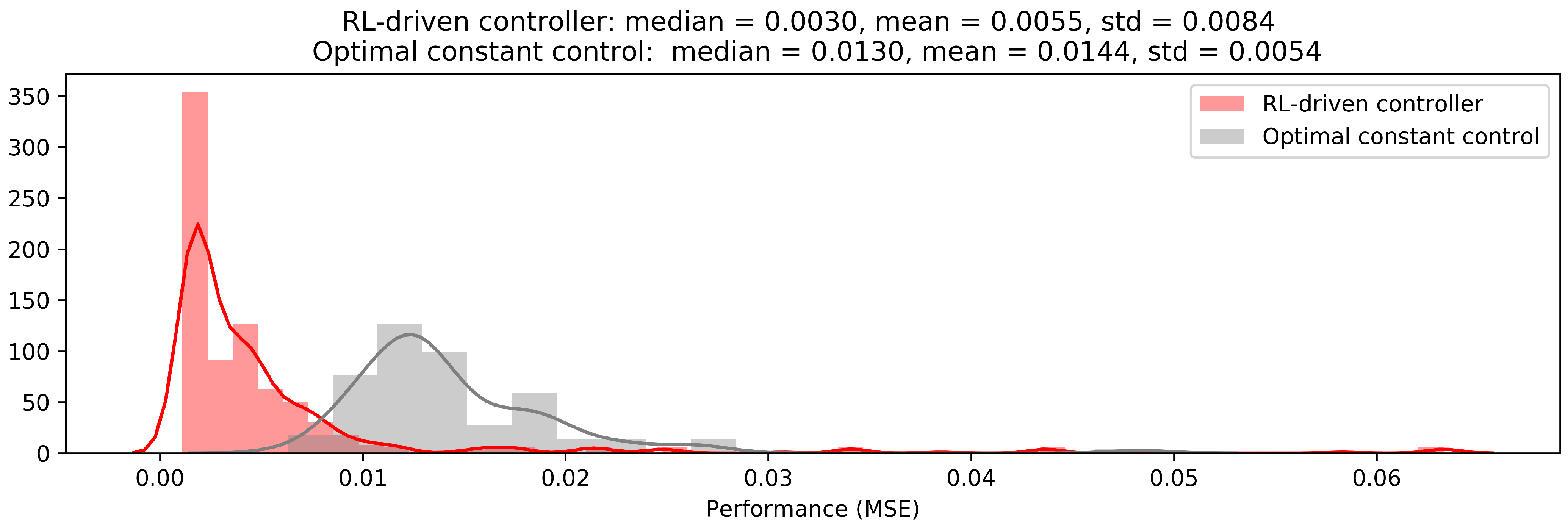
To test the generalization capabilities of the developed RL controller, a setup with a bigger number of TCLs was organized. A comparison of the RL controller’s performance with the competing approach (proportional control) was made using both qualitative and quantitative analyses. Statistical measures (mean, median, and std) collected in the process of the quantitative analysis are presented in Table 3. The competing approach, in this case, has chosen k = 7 as optimal control. The median of the MSE distribution for the proposed solution is more than two times smaller than for the competing approach, the mean is almost two times smaller and even standard deviation is approximately 1.4 times smaller for the proposed RL controller. This indicates that the performance of the proposed approach is significantly better than the proportional control. Moreover, high standard deviation is not observed in the 40 TCLs setup in contrast to the 20 TCLs setup, and thus it can be stated that these observations with high MSE are very rare.
The qualitative analysis represented by the visualization of MSE sample distributions are given in Figure 12. It can be observed that the distribution of MSE samples for the proposed approach (red) is shifted to the left, closer to zero, compared to the distribution of proportional control performance samples (grey). This confirms that the received results of the controller application are aligned with the initial goal because the control goal is to reduce MSE.
The results of the qualitative and quantitative analyses confirm that the presented solution performance is significantly better than the performance of the competing approach for the 40 TCLs setup. A rough estimate is that a proposed solution shows two times better results. Thus, the proposed RL-driven controller works efficiently not only in the 20 TCLs setup, where it was finetuned, but also in the 40 TCLs setup, where it was applied without additional tuning. This is the evidence of the generalization capabilities of the proposed solution.

3.3. Evaluation of the Expected Decrease in Costs

The evaluation of the achieved decrease in costs for considered setups was done to give an intuition of the possible impact of the proposed solution. To calculate the expected decrease in costs, the following assumptions were made: 1 p.u. in the simulated power system equals 1 kW; 1 kWh cost equals USD 0.18—peak hours pricing according to [8]. That is, each 1 kWh of deviation from the reference power profile causes inefficiency in costs equal to USD 0.18.
First, deviation of the actual power consumption and reference power profile was measured in kWh for both the proposed and the competing approaches. The case with no control in the system was not considered, as it is strongly inferior to the competing approach. Second, the positive impact of the RL-driven controller was measured as a decrease in deviation compared to the competing approach. The calculated decrease in deviation of power consumption compared to the competing approach is presented in Table 4. According to the received data, utilization of the RL-driven controller instead of the proportional controller allows us to achieve a 56% decrease in deviation from the planned power profile for the 20 TCLs setup and approximately 39% for the 40 TCLs setup, i.e., after the proposed controller’s application, the actual power consumption is significantly closer to the reference power profile. For a power system setup with 40 TCLs, the change is more modest than for a setup with 20 TCLs. This is due to finetuning that was done for 20 TCLs case, while exactly the same model was applied to the 40 TCLs case and no finetuning was performed.
After calculating the decrease in deviation from the planned power profile, a corresponding decrease in costs was calculated. There may be other improvements in cost efficiency implicitly caused by improvements in a profile of actual power consumption, but this evaluation accounts only for an explicit positive effect of having a power consumption close to the planned profile. The calculated decrease in cost compared to the competing approach is presented in Table 5. Numbers are given in USD × 10 4 for readability, as calculated costs for a 200 s interval considered in the experiment are small.
A significant decrease of costs is achieved for both cases, according to the results. It is important to emphasize that this efficiency is achieved without any significant influence to customers comfort or overriding consumers decisions. This is because of the chosen problem formulation that excludes direct interventions to the consumer side processes and operates using only customer-agnostic information.
However, it can be observed that the decrease of costs for the 40 TCLs setup is smaller than for the 20 TCLs setup. This is because the RL-driven controller was not finetuned for the 40 TCLs case and thus achieved an approximately 17% smaller decrease in the deviation from the planned power profile. This can be improved with additional calibration of the RL-driven controller. Such a calibration can be done by performing hyperparameters tuning for a particular power system setup or performing calibration via a short period of additional training in the power system of interest. Both options are likely to improve performance and, thus, help to achieve higher costs decrease.

4. Conclusions

The proposed solution introduces a DDQN-based approach to provide ancillary services using a set of TCLs by controlling voltage change on a feeder. The presented DDQN controller performs significantly better than the proportional control used as a reference for comparison as a competing approach. While effectively achieving the goal of approaching actual power consumption to the reference power profile, the presented approach aims for customer comfort and does not require any interventions on the consumer side of a power grid.
From the technical point of view, an additional advantage of the DDQN algorithm utilization is the possibility to use continuous input variables without discretizing them. Because of that, the proposed RL-driven controller can be utilized without a sophisticated tuning or configuration in any setup when the corresponding input signals and control actions are available. The high applicability of the approach makes wide utilization possible.
Wide utilization of such ancillary services could help to decrease inefficiencies in terms of costs in the power grid at a global scale. This may be utilized to explicitly decrease consumer electricity costs. In addition, a decrease in actual power consumption profile deviation from the planned one allows keeping a balance of the grid operation. This way, energy resources can be consumed in the optimal and planned way, e.g., the need for unexpected peak energy generation, usually backed up by non-renewable energy sources, will be decreased. This will not only lead to costs optimization but also help to achieve sustainable development goals and reduce harmful effects on the environment often caused by non-renewable energy sources.
As in rare cases, RL-driven controller has shown performance that is not superior to the competing approach, it is worth considering extending controller workflow with a calibration part. That is, after learning a more general version of the optimal control strategy from other similar environments, the controller can be calibrated by additional short training in the specific power system, so that it can adapt to the specific properties of a new environment. To ensure safe functioning in the real world, it also makes sense to help the controller avoid clearly erroneous decisions, e.g., by adding safety measures employing expert knowledge in the power system domain.
In addition, it is reasonable to attempt changing the controller design by aiming to improve performance of the controller. For example, a possible option to improve performance is the employment of consumer-side information. This will require a total reformulation of the considered technical problem and increase the complexity of environment state and action spaces, although this may lead to some improvements in the performance. However, the applicability of such an approach is limited, as it can be utilized only if most TCL devices are equipped with smart technologies and proper authorization is received for information gathering and/or consumer-side actions from all the corresponding customers.

Author Contributions

Methodology, O.L. and T.B.; writing—original draft preparation, O.L.; writing—review and editing, T.B.; supervision, T.B. All authors have read and agreed to the published version of the manuscript.

Funding

This research was funded by ELEKS (https://eleks.com/ (accessed on 31 March 2021)) via funding by the Machine Learning Lab at the Ukrainian Catholic University.

Data Availability Statement

The research data and code utilized for experiments are stored in a GitHub repository [35].

Conflicts of Interest

The authors declare no conflict of interest.

Abbreviations

The following abbreviations are used in this manuscript:
TCLThermostatically Controlled Loads
IoTInternet of Things
RLReinforcement Learning
DQNDeep Q-network
DDQNDouble Deep Q-network
MSEMean Squared Error
SOTAState-of-the-Art
stdstandard deviation

Appendix A. Nomenclature Table

Table A1. Nomenclature table of the variables mentioned in the paper.
VariableDescriptionUnits
θ temperature of TCL°C
θ m i n lower temperature threshold in TCL°C
θ m a x upper temperature threshold in TCL°C
θ a ambient temperature°C
ttimes
T h time of TCL heatings
T c time of TCL coolings
APLactual power levelper units (p.u.) or W
RPLreference power levelper units (p.u.) or W
Ppowers, consumptionper units (p.u.) or W
Rthermal resistance of TCL°C/kW
vvoltageV
g 0 conductance 1 / Ω
Cthermal capacitance of TCL-
rangewidth of TCLs thermal capacities range-
urandom number from uniform distribution in [ 0 ; 1 ] -
s w i t c h binary indicator if TCL is on (1) or off (0)-
sstate of the environment-
aagent’s action-
Q ( s ; a ) Q-value function-
V ( s ) state value function-
R ( s ; a ) reward function-
pprobability-
γ discount factor-

References

  1. Callaway, D.S. Tapping the energy storage potential in electric loads to deliver load following and regulation, with application to wind energy. Energy Convers. Manag. 2009, 50, 1389–1400. [Google Scholar] [CrossRef] [Green Version]
  2. Begovic, M.; Pregelj, A.; Rohatgi, A.; Novosel, D. Impact of renewable distributed generation on power systems. In Proceedings of the 34th Annual Hawaii International Conference on System Sciences, Maui, HI, USA, 3–6 January 2001; IEEE: Piscataway, NJ, USA, 2001; pp. 654–663. [Google Scholar]
  3. Mahmud, N.; Zahedi, A. Review of control strategies for voltage regulation of the smart distribution network with high penetration of renewable distributed generation. Renew. Sustain. Energy Rev. 2016, 64, 582–595. [Google Scholar] [CrossRef]
  4. Xu, X.; Yan, Z.; Shahidehpour, M.; Wang, H.; Chen, S. Power system voltage stability evaluation considering renewable energy with correlated variabilities. IEEE Trans. Power Syst. 2017, 33, 3236–3245. [Google Scholar] [CrossRef]
  5. Stojkoska, B.L.R.; Trivodaliev, K.V. A review of Internet of Things for smart home: Challenges and solutions. J. Clean. Prod. 2017, 140, 1454–1464. [Google Scholar] [CrossRef]
  6. Ipakchi, A.; Albuyeh, F. Grid of the future. IEEE Power Energy Mag. 2009, 7, 52–62. [Google Scholar] [CrossRef]
  7. El-Bayeh, C.Z.; Eicker, U.; Alzaareer, K.; Brahmi, B.; Zellagui, M. A Novel Data-Energy Management Algorithm for Smart Transformers to Optimize the Total Load Demand in Smart Homes. Energies 2020, 13, 4984. [Google Scholar] [CrossRef]
  8. Wang, B.; Li, Y.; Ming, W.; Wang, S. Deep reinforcement learning method for demand response management of interruptible load. IEEE Trans. Smart Grid 2020, 11, 3146–3155. [Google Scholar] [CrossRef]
  9. Rehman, A.U.; Lie, T.T.; Vallès, B.; Tito, S.R. Non-Intrusive Load Monitoring of Residential Water-Heating Circuit Using Ensemble Machine Learning Techniques. Inventions 2020, 5, 57. [Google Scholar] [CrossRef]
  10. Silver, D.; Huang, A.; Maddison, C.J.; Guez, A.; Sifre, L.; Van Den Driessche, G.; Schrittwieser, J.; Antonoglou, I.; Panneershelvam, V.; Lanctot, M.; et al. Mastering the game of Go with deep neural networks and tree search. Nature 2016, 529, 484–503. [Google Scholar] [CrossRef]
  11. Vinyals, O.; Babuschkin, I.; Chung, J.; Mathieu, M.; Jaderberg, M.; Czarnecki, W.M.; Dudzik, A.; Huang, A.; Georgiev, P.; Powell, R.; et al. AlphaStar: Mastering the Real-Time Strategy Game StarCraft II; DeepMind Technologies Limited: London, UK, 2021. [Google Scholar]
  12. Riedmiller, M.; Gabel, T.; Hafner, R.; Lange, S. Reinforcement learning for robot soccer. Auton. Robot. 2009, 27, 55–73. [Google Scholar] [CrossRef] [Green Version]
  13. Bui, V.H.; Hussain, A.; Kim, H.M. Double deep Q-learning-based distributed operation of battery energy storage system considering uncertainties. IEEE Trans. Smart Grid 2019, 11, 457–469. [Google Scholar] [CrossRef]
  14. Ernst, D.; Glavic, M.; Capitanescu, F.; Wehenkel, L. Reinforcement learning versus model predictive control: A comparison on a power system problem. IEEE Trans. Syst. Man Cybern. Part B 2008, 39, 517–529. [Google Scholar] [CrossRef]
  15. Ma, O.; Alkadi, N.; Cappers, P.; Denholm, P.; Dudley, J.; Goli, S.; Hummon, M.; Kiliccote, S.; MacDonald, J.; Matson, N.; et al. Demand Response for Ancillary Services. IEEE Trans. Smart Grid 2013, 4, 1988–1995. [Google Scholar] [CrossRef]
  16. Heffner, G. Loads Providing Ancillary Services: Review of International Experience. 2008. Available online: https://escholarship.org/uc/item/0jj524xw (accessed on 31 March 2021).
  17. Meyn, S.P.; Barooah, P.; Bušić, A.; Chen, Y.; Ehren, J. Ancillary service to the grid using intelligent deferrable loads. IEEE Trans. Autom. Control. 2015, 60, 2847–2862. [Google Scholar] [CrossRef] [Green Version]
  18. Zhang, W.; Kalsi, K.; Fuller, J.; Elizondo, M.; Chassin, D. Aggregate model for heterogeneous thermostatically controlled loads with demand response. In Proceedings of the 2012 IEEE PES General Meeting, San Diego, CA, USA, 22–26 July 2012; pp. 1–8. [Google Scholar]
  19. Kirby, B.; Hirst, E. Load as a Resource in Providing Ancillary Services; Lockheed Martin Energy Research, Oak Ridge National Laboratory: Oak Ridge, TN, USA, 1999.
  20. Pallonetto, F.; De Rosa, M.; Milano, F.; Finn, D.P. Demand response algorithms for smart-grid ready residential buildings using machine learning models. Appl. Energy 2019, 239, 1265–1282. [Google Scholar] [CrossRef]
  21. Claessens, B.J.; Vanhoudt, D.; Desmedt, J.; Ruelens, F. Model-free control of thermostatically controlled loads connected to a district heating network. Energy Build. 2018, 159, 1–10. [Google Scholar] [CrossRef] [Green Version]
  22. Tindemans, S.H.; Trovato, V.; Strbac, G. Decentralized control of thermostatic loads for flexible demand response. IEEE Trans. Control. Syst. Technol. 2015, 23, 1685–1700. [Google Scholar] [CrossRef]
  23. Bogodorova, T.; Vanfretti, L.; Turitsyn, K. Voltage control-based ancillary service using thermostatically controlled loads. In Proceedings of the 2016 IEEE Power and Energy Society General Meeting (PESGM), Boston, MA, USA, 17–21 July 2016; IEEE: Piscataway, NJ, USA, 2016; pp. 1–5. [Google Scholar]
  24. Lukianykhin, O.; Bogodorova, T. Reinforcement Learning for Thermostatically Controlled Loads Control using Modelica and Python. In Proceedings of the Asian Modelica Conference 2020, Tokyo, Japan, 8–9 October 2020; pp. 31–40. [Google Scholar]
  25. Moriyama, T.; De Magistris, G.; Tatsubori, M.; Pham, T.H.; Munawar, A.; Tachibana, R. Reinforcement Learning Testbed for Power-Consumption Optimization. In Asian Simulation Conference; Springer: Singapore, 2018; pp. 45–59. [Google Scholar]
  26. Mottahedi, S. Battery Energy Management System Using Reinforcement Learning. 2017. Available online: https://github.com/smottahedi/RL-Energy-Management/blob/master/presentation.ipynb (accessed on 31 March 2021).
  27. Lukianykhin, O.; Bogodorova, T. ModelicaGym: Applying reinforcement learning to Modelica models. In Proceedings of the 9th International Workshop on Equation-based Object-Oriented Modeling Languages and Tools, Berlin, Germany, 5 November 2019; pp. 27–36. [Google Scholar] [CrossRef] [Green Version]
  28. Chen, W.; Huhn, M.; Fritzson, P. A Generic FMU Interface for Modelica. In Proceedings of the 4th International Workshop on Equation-Based Object-Oriented Modeling Languages and Tools, ETH Zurich, Switzerland, 5 September 2011. [Google Scholar]
  29. Vázquez-Canteli, J.R.; Nagy, Z. Reinforcement learning for demand response: A review of algorithms and modeling techniques. Appl. Energy 2019, 235, 1072–1089. [Google Scholar] [CrossRef]
  30. Ruelens, F.; Claessens, B.J.; Quaiyum, S.; De Schutter, B.; Babuška, R.; Belmans, R. Reinforcement learning applied to an electric water heater: From theory to practice. IEEE Trans. Smart Grid 2016, 9, 3792–3800. [Google Scholar] [CrossRef] [Green Version]
  31. Brockman, G.; Cheung, V.; Pettersson, L.; Schneider, J.; Schulman, J.; Tang, J.; Zaremba, W. OpenAI Gym. arXiv 2016, arXiv:1606.01540. [Google Scholar]
  32. Van Rossum, G.; Drake, F.L., Jr. Python Tutorial; Centrum v. Wiskunde en Informatica Amst.: Amsterdam, The Netherlands, 1995; Volume 620. [Google Scholar]
  33. Fritzson, P. Principles of Object-Oriented Modeling and Simulation with Modelica 3.3: A Cyber-Physical Approach; John Wiley & Sons: Hoboken, NJ, USA, 2014. [Google Scholar]
  34. Lukianykhin, O.; Bogodorova, T. Ucuapps/Modelicagym: Modelica Models Integration with Open AI Gym. 2019. Available online: https://github.com/ucuapps/modelicagym (accessed on 31 March 2021).
  35. Lukianykhin, O.; Bogodorova, T. OlehLuk/Deeprl-Demand-Response: DDQN-Driven Voltage Controller for Ancillary Service. 2021. Available online: https://github.com/OlehLuk/deeprl-demand-response (accessed on 31 March 2021).
  36. Mnih, V.; Kavukcuoglu, K.; Silver, D.; Rusu, A.A.; Veness, J.; Bellemare, M.G.; Graves, A.; Riedmiller, M.; Fidjeland, A.K.; Ostrovski, G.; et al. Human-level control through deep reinforcement learning. Nature 2015, 518, 529–533. [Google Scholar] [CrossRef] [PubMed]
  37. Van Hasselt, H.; Guez, A.; Silver, D. Deep Reinforcement Learning with Double q-Learning. Proc. Aaai Conf. Artif. Intell. 2016, 30. Available online: https://ojs.aaai.org/index.php/AAAI/article/view/10295 (accessed on 31 March 2021).
  38. Mnih, V.; Kavukcuoglu, K.; Silver, D.; Graves, A.; Antonoglou, I.; Wierstra, D.; Riedmiller, M. Playing atari with deep reinforcement learning. arXiv 2013, arXiv:1312.5602. [Google Scholar]
  39. Sutton, R.S.; Barto, A.G. Reinforcement Learning: An Introduction; MIT Press: Cambridge, MA, USA, 2018. [Google Scholar]
  40. Ioffe, S.; Szegedy, C. Batch normalization: Accelerating deep network training by reducing internal covariate shift. In Proceedings of the International Conference on Machine Learning, PMLR, Lille, France, 6–11 July 2015; pp. 448–456. [Google Scholar]
  41. Andersson, C.; Åkesson, J.; Führer, C. Pyfmi: A python Package for Simulation of Coupled Dynamic Models with the Functional Mock-Up Interface; Centre for Mathematical Sciences, Lund University: Lund, Sweden, 2016. [Google Scholar]
  42. Goodfellow, I.J.; Shlens, J.; Szegedy, C. Explaining and harnessing adversarial examples. arXiv 2014, arXiv:1412.6572. [Google Scholar]
  43. Brown, T.B.; Mané, D.; Roy, A.; Abadi, M.; Gilmer, J. Adversarial patch. arXiv 2017, arXiv:1712.09665. [Google Scholar]
Figure 1. High-level overview of a problem formulation.
Energies 14 02274 g001
Figure 2. The approach of the proposed voltage control-based ancillary service and its interaction flows in the power system.
Energies 14 02274 g002
Figure 3. Diagram of a simulated power system (20 TCLs).
Energies 14 02274 g003
Figure 4. TCL temperature dynamics and power consumption cycle.
Energies 14 02274 g004
Figure 5. TCL heating cycle dependency on thermal capacitance and voltage.
Energies 14 02274 g005
Figure 6. Histogram of TCLs’ (n = 40) proportion that remain ON in a simulated time interval of 200 s.
Energies 14 02274 g006
Figure 7. TCLs’ proportion that remain ON in a simulated time interval of 200 s.
Energies 14 02274 g007
Figure 8. Power consumption range in a time interval of 200 s with a dependency on the thermal capacitance of 40 TCLs.
Energies 14 02274 g008
Figure 9. Smoothed MSE for the episode as a measure of the controller’s performance during training repeat (grey) and summarized (red).
Energies 14 02274 g009
Figure 10. Actual and reference power level example for a trained controller and the competing approach.
Energies 14 02274 g010
Figure 11. Performance metric (MSE) distribution for the developed RL controller and the competing approach (proportional control) for the 20 TCLs setup.
Energies 14 02274 g011
Figure 12. Performance metric (MSE) distribution for the developed RL controller and the competing approach (proportional control) for the 40 TCLs setup.
Energies 14 02274 g012
Table 1. The chosen hyperparameters after the DQN tuning.
ParameterValueValues Considered in Hyperparameters Tuning
Number of hidden layers2was not tuned
Hidden layer size128 [ 32 ; 64 ; 128 ; 256 ]
Batch size32 [ 32 ; 64 ; 256 ]
Replay buffer size256 [ 256 ; 512 ; 1024 ; 2048 ]
Learning rate0.001 [ 0.001 , 0.0001 ]
OptimizerAdamwas not tuned
Target network update step10 [ 1 ; 10 ; 100 ; 1000 ; 10,000 ]
Table 2. Performance comparison in terms of MSE statistical properties for the proposed solution and the competing approach (proportional control) for 20 TCLs feeder.
MethodMedianMeanStd
No control0.05460.06130.0196
Competing approach ( k = 7 )0.0130.01440.0054
Best Double DQN0.00300.00550.0084
Table 3. Performance comparison for 40 TCLs setup.
MethodMedianMeanStd
Competing approach ( k = 7 )0.01730.01870.0064
Best Double DQN0.00850.010.0045
Table 4. Achieved decrease in deviations of actual power consumption from the reference power profile compared to the competing approach (proportional control) for 200 s period, in kWs.
MethodMedianMeanStdTotal for 100 EpisodesRelative Change
Best DDQN (20 TCLs setup)11.7112.143.491171.0956.04%
Best DDQN (40 TCLs setup)9.779.034.73903.1738.89%
Table 5. Achieved decrease in costs compared to the competing approach (proportional control) for 200 s period, in USD × 10 4 .
MethodMedianMeanStdTotal for 100 Episodes
Best DDQN (20 TCLs setup)5.8556.071.745585.545
Best DDQN (40 TCLs setup)4.8854.5152.365451.585
Publisher’s Note: MDPI stays neutral with regard to jurisdictional claims in published maps and institutional affiliations.

