A Multiphysics Analysis of Coupled Electromagnetic-Thermal Phenomena in Cable Lines

Abstract

The paper is focused on numerical modeling of multi-strand cable lines placed in free air. Modeling is carried out within the framework of the so-called multi-physics approach using commercial software. The paper describes in detail the steps undertaken to develop realistic, reliable numerical models of power engineering cables, taking into account their geometries and heat exchange conditions. The results might be of interest to the designers of multi-strand cable systems.

1. Introduction

1.1. General Remarks

Energy transfer in low voltage networks and installations is in many cases related to flow of currents with significant values. This issue occurs for example in the lines connecting medium voltage (MV) transformers to main switchgears of industrial entities as well as in the installations of high storey buildings. The necessity to deliver high amounts of energy requires that current-leading tracks with significant ampacities (current carrying capacities) are used. Usually such connections are made of bare bars or insulated bus-bars. The design of these components has been described in detail in several publications, cf. e.g., [1,2]. In some cases due to economical reasons (this is true in particular for insulated bus-bars) or technical limitations (resulting from the geometry of the devices) it is not possible to consider the connections made of bare bars. An alternative solution might be the design of current tracks made of several single strand cables per phase, connected in parallel, cf. Figure 1. This solution is simpler to be implemented, more flexible, moreover it is much cheaper than the use of insulated bus-bars. Unfortunately, this solution is not devoid of deficiencies. In many cases it can happen that the individual strands connected in parallel are subject to non-uniform current distribution. This effect may lead to a significant temperature increase in the overloaded strands, sometimes exceeding the long-lasting admissible values, which in turn may lead to shortening of cable insulation service “life” [3] and under certain unfavorable conditions it may lead to cable malfunction or insulation breakdown.

The non-uniform current distribution in individual strands depends on their spatial configuration as well as on other phenomena. On the other hand the spatial configuration affects the mutual couplings between conductors leading currents (skin and proximity phenomena related to the flow of eddy currents generated in the strands) [4]. Analytical handling of these effects is rather difficult even for simple geometries. Quite recently Jabłoński et al. presented a hybrid approach to compute skin and proximity effects for two parallel conductors with circular cross section based on the method of successive reactions [5]. The approach was extended to take into account the couplings in three phase lines with round conductors in reference [6].

The present paper is complementary to the previous work [7]. The aforementioned publication introduced a simplified approach to assess the optimal current distribution in low-voltage multi-strand cable lines, whereas the present contribution focuses on coupled electromagnetic-thermal modeling using commercial software. The previous contribution introduced a simple criterion based on barycenter location of individual strands, which might help the designer to choose those spatial configurations for which the skin and proximity effects might be mitigated. The criterion may be easily implemented in a popular spreadsheet, or even checked using “by-hand” computations, thus there is no need to resort to sophisticated software tools like e.g., the Vector Immune Optimization method [8,9,10,11] or other global optimization algorithms [12,13,14,15,16,17,18]. However, as pointed in the Conclusion section of the paper [7], the final step of the design stage should be based on FEM computations that take into account the coupled electromagnetic-thermal phenomena. The present contribution thus fills the gap in this respect and provides additional information. Both papers have been compiled from Ph.D. Thesis [19]. The following modeling aspects are covered in this contribution:

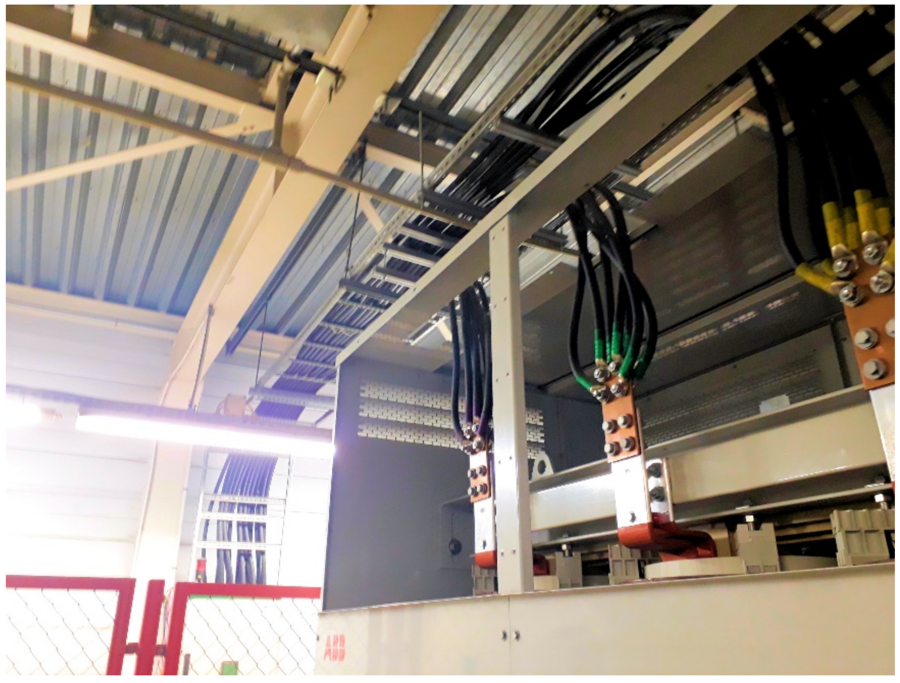
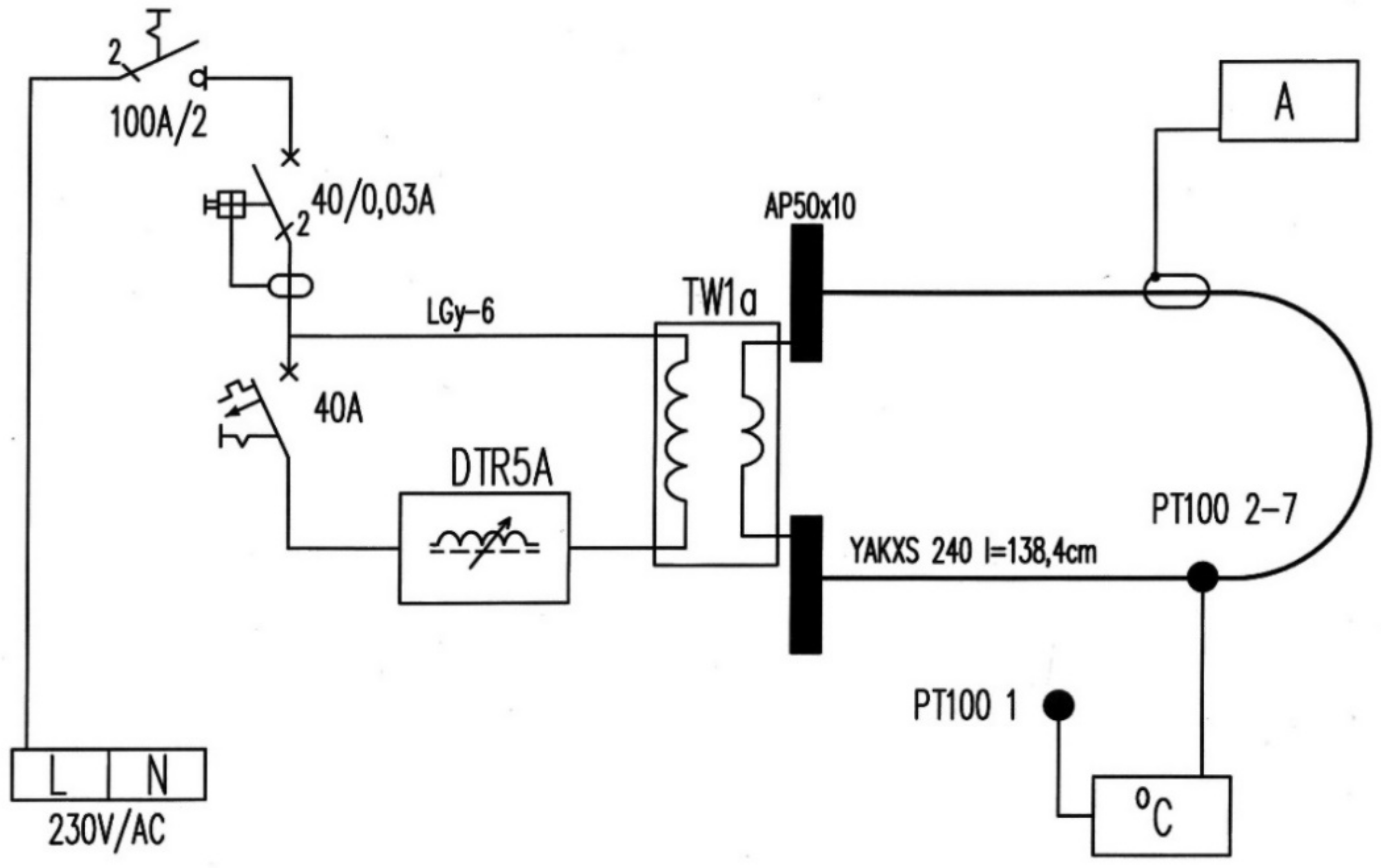
• description of a laboratory stand for examination of current distribution in multi-strand lines,
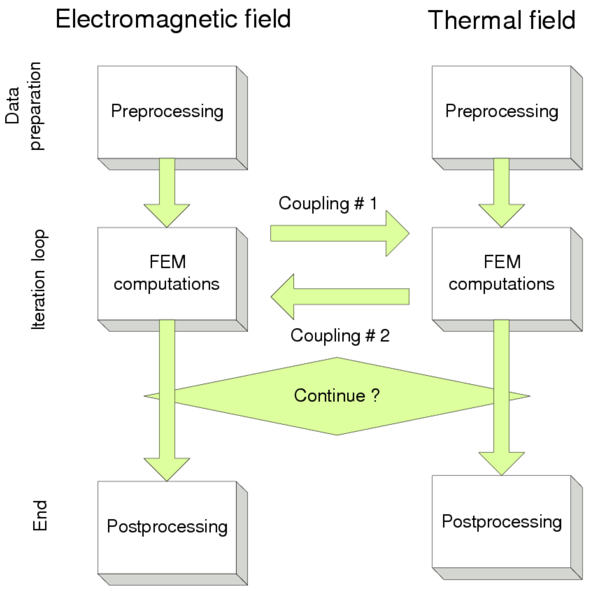
• development of a numerical model taking into account coupled electromagnetic-thermal phenomena,
• comparison of computation results from ICEPACK and MAXWELL-MECHANICAL codes for chosen geometries,
• variations of temperature and RMS current values during successive iterations using the coupled electromagnetic-thermal model.

The paper is focused on the so-called multiphysics modeling, thus in this section a brief description of the concept is provided. As pointed out by Driesen [20] in order to predict correctly the behavior of a technical device, several phenomena have to be taken into account in engineering analysis and design. In fact, quite often we face the need to consider several physical phenomena occurring on different time- and spatial scales in order to maintain a correct description of reality. In solid state physics this may be achieved e.g., by using the concept of “effective field” [21,22,23]. Figure 2 depicts field interactions in a general electromagnetic problem.

The term “multiphysics” implies an emerging interdisciplinary study area, that considers several simultaneously occurring physical fields and focuses on the studies of and knowledge about these processes and systems [24,25,26,27]. Multiphysics approach to modeling means that phenomena like heat transfer, electromagnetic and mechanical effects are taken into account for the considered material or device. State-of-the-art computers are powerful enough to carry out sophisticated calculations thus the issue has attracted much attention recently. Modeling is carried out using different time and spatial scales and the examined structure might be considerably complex [28,29,30,31,32].

In the context of cable modeling the paper by Chávez et al. [33] might be a good example of the multiphysics approach. In the aforementioned paper the authors have developed a theoretical model to study the combined effects of electromagnetic and thermal fields on cable ampacity, which takes into account the dependence of resistivity on temperature.

1.2. Literature Review Concerning Ampacity Computation

In engineering practice the Finite Element Method (FEM) is the prevailing numerical technique to solve partial differential equations that describe phenomena occurring in power cables. Analytical approaches aimed at determination of cable ampacities have a limited application scope, since they may be applied only for simple geometries and in homogeneous ambient conditions [34]. From literature review it follows that the analysis of coupled electromagnetic and thermal fields for simpler geometries at in-door conditions has been considered by several authors. It should however be remarked that in practice much more attention is paid to the analysis of buried cables [3,34,35].

De León presented a parametric study of the effects of conductor size, cable grouping, and heat exchange conditions, that affect cable ampacity (current carrying capability) both for cables laid in free air and for buried ones [36]. Sedaghat and de León [37] have carried out computations of steady-state temperature of power cables in free air for the most common spatial configurations and compared their results to those resulting from the IEC-60287-2-1 standard [38]. The books [39,40] are comprehensive sources of information on the issues related to power cable rating and design.

For ampacity calculations in multi-strand cable lines placed in free air at indoor conditions (when it is possible to neglect the fluid flow affecting heat transfer conditions) the mutual coupling between electromagnetic and thermal fields is of paramount importance. Goga et al. carried out numerical computations concerning cooling of a single electrical conductor with insulation [41]. Li and coworkers computed temperature distribution and power losses for typical (flat and trefoil) three phase single strand cable configurations using a simplified 2D FEM cable model [42]. Cirino et al. focused on the problem how the cable parameters used in FEM calculations are affected by skin and proximity effects [43]. Korovkin et al. presented several possible modeling strategies regarding ampacity modeling using FEM for buried cables [44]. The conclusions drawn by the authors are consistent with the general statements on coupled problems made earlier by Hameyer et al. [45], namely for the considered problem the thermal and electromagnetic time scales differ significantly. The electromagnetic part may be coupled to the heat transfer part either by a one-way link (the generated Ohmic losses are simply transferred as input to the thermal model) or by two-way links, if subsequently the effect of temperature on conductivity is accounted.

In the present work electromagnetic and thermal phenomena are coupled using the two-way method, the computations were repeated in a loop until transient phenomena faded away. At least three iterations were needed for this purpose. The flowchart of the computation routines is depicted in Figure 3.

For the case of buried cables there are additional problems due to soil inhomogeneity [35,36,46,47] and heat exchange conditions between the cable shield and the soil or the backfill material [36,39,46,48,49,50].

2. Materials and Methods

In the paper [7] a brief description of a laboratory stand used for practical experiments with chosen single-phase systems was given. In order not to repeat the description we include here only new relevant pieces of information. For physical modeling single-stranded YAKXS-type cables were used (diameters 70 mm² and 240 mm²). The strand was made of aluminum, insulation—of cross-linked polyethylene (XLPE) and the coating—of polyvinyl chloride, cf. Figure 4.

Table 1. Parameters of the examined cables.

	YAKXS 1 × 240	YAKXS 1 × 70
Working aluminum strand—RMC	240 mm2	70 mm2
Insulation—cross-linked polyethylene	1.7 mm	1.1 mm
Coating—polyvinyl chloride	1.7 mm	1.4 mm
Outer diameter	24.8 mm	14.7 mm
Maximum resistance at 20 °C	0.125 Ω/km	0.443 Ω/km
Maximum working temperature	90 °C	90 °C

includes the basic information on the examined cables.

The value of the outer diameter was verified experimentally. For chosen sections 15 measurements were made with a digital slide caliper (resolution 0.03 mm) in different points. The following results were obtained for the YAKXS $1\times 240$ cable: 25.71; 26.23; 25.51; 25.61; 25.52; 25.74; 26.11; 25.83; 25.71; 26.23; 25.51; 25.61; 26.12; 25.54; 25.65 mm. The average outer diameter was 25.77 ± 0.03 mm.

A fragment of YAKXS $1\times 240$ cable, 138.4 cm long (the terminals not taken into account), with resistance 176.75 µΩ, was excited with the 608 A current (Root Mean Square). This current value was the maximum long-lasting admissible one for this type of cable, according to the producer data. Resistance measurements were carried out using the technical method, using a DC supply source (EMEX 400 DC), with the nominal current equal to 400 A. Voltage measurements were made with a digital voltmeter Fluke 177 using the range 0.1–600 mV. The accuracy of the measurement: 0.09% + 2 digits. The excitation was achieved using the transformer TW1a (220 V, 1 kVA) and the coil DTR4a used for adjusting the current value. The current values were recorded with the PQM-701Z analyzer from Sonel with the use of Rogowski’s coils (I_n = 1000 A, minimal fundamental accuracy 1%, according to the producer).

The electrical connection scheme is depicted in Figure 5. At this point it can be remarked that a similar circuit was used by the authors of reference [51].

3. Numerical Modeling

For computations the commercial ANSYS Maxwell software [52] was used. The piece of software makes it possible to model low frequency electromagnetic field phenomena using FEM for solving Maxwell equations. The design of two- and three-dimensional systems, considering skin and proximity effects is also possible. Integration in the ANSYS Workbench allows one to carry out coupled analyses with the use of appropriate mechanical and flow modules. The coupled analyses describe more precisely such phenomena as e.g., the change in conductivity of the working strand upon temperature increase or cable heating being the result of induced eddy currents.

Model assumptions were as follows:

• modeling was carried out for 2D geometry. The full 3D modeling is possible in ANSYS, yet it is very time consuming; some tests carried out by the first author have shown that it may take several hours even for relatively simple geometries using a state-of-the-art desktop computer;
• individual strands twisted together to form a cable line (cf. Figure 2) are treated as a whole. This simplification may be called a geometric homogenization on the local scale. The proximity effects are accounted only between “clusters” of strands from the macroscopic standpoint. It can be remarked that this approach is a typical one; yet a recent publication on the wiring system for electrical vehicles focused on a more detailed scale [53];
• the cables are cooled by natural convection. It is assumed that their distance from the floor is sufficient to neglect the floor heating due to radiation emitted from the cables.

The geometry for the analysis was prepared directly in ANSYS Maxwell on the basis of real-life dimensions and materials used in the analyzed cables. Figure 6 depicts the geometrical model of a single strand made of aluminum, XLPE insulation and outer coating made of polyvinyl chloride in a six stranded cable. The second part of the Figure illustrates the considered setup. The values for conductivity and resistance temperature coefficient assumed in computations for aluminum were assumed as 34.8 MS/m and 0.0041 deg⁻¹, respectively.

Taking into account the boundary conditions and requirements concerning field analysis, the cables were encompassed with the air domain, as shown in Figure 7. The domain was prepared in such a way, so that it did not influence the values of magnetic field strength. On its outer boundaries the Baloon boundary condition was preset.

The analysis was made with the Magnetic Transient solver, which makes it possible to monitor instant values of magnetic field intensity. In order to obtain more realistic results the contact resistances for cable terminals were included in the equivalent connection diagram, cf. Figure 8 (the word “zaciski” in Polish stands for “terminals”). It seems important to stress that Maxwell Circuit Editor presented in the Figure allows one to consider different excitation scenarios in a straightforward way, for example if one is interested in FEM analysis for excitation currents with significant harmonic contents, one has to add additional branches containing sources with appropriately chosen amplitudes and frequencies in parallel to the fundamental supply branch denoted as I0. It is important to stress that in real life conditions the dependencies i(t) might indeed be distorted [54].

Determination of Free Convection Coefficient and Modeling

In order to determine the maximum temperature achieved by the cable with current as well as the temperature distribution inside the cable it is necessary to determine the value of free convection coefficient as well as the correct values of thermal conductivity for individual layers (insulation and coating). A correct value of radiation coefficient has also to be supplied to the software.

For a single strand the heating tests with the maximal long-lasting admissible current were carried out. On their basis the value of the free convection coefficient was determined from Newton law. The obtained results were compared to the values from simulations from the ICEPACK module from the ANSYS suite. The estimated values of free convection coefficient, thermal conductivities of outer cable layers and radiation coefficient were introduced into the coupled Maxwell-Mechanical module in order to carry out a verification and a comparison with experimental results from the laboratory stand.

Ambient and strand temperatures were recorded using an eight-channel temperature recorder (AR208 from Apar), equipped with platinum temperature sensors (PT100). These sensors feature high stability of physical properties. In order to increase the measurement sensitivity, the connection of sensor to the examined cable fragment was made using a silver-based conductive paste Zalman STG-2, whereas the attachment to the cable surface was made using a silicon tape. Figure 9 depicts the location of temperature measurement points.

Temperature measurements were carried out every 30 s. There were 377 data samples that were recorded until the strand and coating temperatures achieved the steady state. The tests lasted 188 min. The obtained heating curves for the YAKXS $1\times 240$ cable is depicted in Figure 10. Similar heating tests for a single bare aluminum cable were reported recently by Kasaš-Lažetić et al. [55].

During the measurements the ambient temperature changed from 22.1 up to 24.1 °C. The following temperature values were achieved in the steady state:

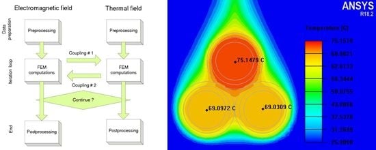
• the working strand—79.0 °C
• insulation—69.8 °C
• outer coating (measurement point below the strand)—62.0 °C
• outer coating (measurement point above the strand)—67.1 °C

The value of natural convection coefficient was determined using the Neher-McGrath method [39,56]. The measurements were carried out in a closed room, therefore the effects of heating from solar rays as well as from forced air flow were neglected. Considering the measured cable length and strand diameter the surface area was calculated. It was equal to 0.112 m². Because the strand temperature varied from 62.0 to 67.1 °C along the perimeter, the average value 64.55 °C was assumed for further calculations. The computed value of natural convection coefficient was equal to h = 10.5 W/(m² K).

The following values were assumed for the model developed in the ICEPACK module:

−

unit loss per 1 cm length was calculated in Maxwell using the 3D model, it was equal to 0.557 W;

−

the values of thermal conductivity coefficients were taken from relevant materials science publications. They were as follows: PVC = 0.17 W/(m K), XPLE = 0.52 W/(m K) and ALU = 237 W/(m K). The radiation coefficient was 0.94. The ambient temperature was assumed as 26.1 °C.

The dependencies temperature vs. iteration number for the working strand (red) and for the outer coating (upper part—blue, lower part—green) are depicted in Figure 11.

Temperature distribution across the cable cross-section, considering the individual layers is depicted in Figure 12. The steady-state temperature values are as follows: for the working strand 79.2 °C, for outer coating (measurement point below the strand)—61.6 °C, for outer coating (measurement point above the strand)—67.9 °C, for insulation—76.2 °C. On the basis of carried out measurements the value of free convection coefficient was determined. It was equal to 10.2 W/(m² K).

The computed value of free convection coefficient and the confirmed experimentally values of thermal conductivity and radiation were subsequently assumed for computations carried out in the MAXWELL-MECHANICAL module for coupled computations. The results of coupled computations for current value 608 A (RMS) and initial ambient temperature 24 °C are depicted in Figure 13.

Comparing the results obtained from developed models to those from real-life measurements it can be stated that a reasonable accuracy of the models has been achieved. For subsequent analysis of more complicated spatial configurations the coefficient values describing material properties for the single strand are assumed. In Figure 14 and Figure 15 the FEM computation results are shown for the trefoil configuration, which is quite commonly found in practice. In Figure 14 the results for congested configuration are depicted, whereas in Figure 15 the cables are set apart, the distance between individual strands is equal to the outer cable diameter. Temperature values computed with both approaches for the strand centers are quite similar (the discrepancies are below 1%), yet it should be remarked that FEM computations made with the ANSYS-MECHANICAL coupled module last significantly longer. On the other hand, the graphics obtained with ICEPACK provide more information, since one can read out local ambient temperature values.

It can be noticed that for the trefoil geometry when the cables are set apart, all strands attain practically the same maximal temperature (around 54 deg), which means that favorable heat exchange conditions were achieved. However in practice due to space limitations it is sometimes necessary to use the congested geometry (Figure 14), which may lead to excessive heating of the upmost strand resulting from convection.

As a representative example for the practical application of the presented method the results of coupled computations are provided for three spatial configurations (two cables per phase) considered previously in reference [7]. Some configurations (e.g., the two-row setup ABC/ABC) are not favorable, since they violate the barycenter criterion for uniform current distribution provided in the aforementioned paper. In fact, the computation results indicate that in this case the maximum temperature in the system (obtained for phase B) may indeed exceed the admissible value and thus a system malfunction may occur. It is interesting to remark that Al-Ohaly et al. arrived at similar conclusions in reference [57]. These authors who compared voltages and dissipated power losses for double flat configurations ABC/ABC and ABC/CBA using impedance matrix formulation and indicated the latter configuration as favorable one.

Figure 16 depicts the computed distributions of (a) power density and (b) temperature in the considered setup, whereas

Table 2. Computation results for chosen configurations.

	A1B1C1A2B2C2		A1B1C1/C2B2A2		A1B1C1/A2B2C2
	P (W)	Tmax (°C)	P (W)	Tmax (°C)	P (W)	Tmax (°C)
A1	22.91		24.73		24.48
B1	24.61		25.19	90.85	26.87	93.3
C1	24.27	74.1	24.40		24.52
A2	22.91	-	24.37		24.53
B2	24.61	-	25.21	90.85	26.89	93.3
C2	24.26	74.1	24.40		24.49
ΣP [W]	-	143.57	-	148.3	-	151.78

summarizes the computation results for three chosen configurations.

In order to illustrate the necessity to carry out iterative computations of coupled electromagnetic-thermal phenomena for practical scenarios we focus on temperature distribution for a six strand flat configuration supplied from a single phase, cf. Figure 17.

For computations the value of ambient temperature T_amb = 25 °C was used as the starting value for computation of aluminum conductivity in the MAXWELL module. In accordance with the assumed algorithm the computed current values after the first iteration were imported to the thermal module and subsequently the temperature attained by individual strands was computed. The highest temperature values (90.3 °C) were obtained for the strands at the edges (I_RMS = 722 A), the lowest ones (52.1 °C)—for the strands in the middle (I_RMS = 329 A). The temperature distribution after the first and the last iteration is shown in Figure 18.

For the computed temperature values, new instant values of conductivity for each strand was determined and the computations were repeated iteratively (three iterations) until the temperature values attained steady state. It can be noticed that the maximal temperature for the strands at the edges raised up to the value 103 °C. This is an important remark since for the YAKXS cables with cross-linked polyethylene (XLPE) insulation the maximal long-lasting admissible temperature is 90 °C. Therefore it can be remarked that these strands might be destroyed during operation due to excessive heating.

Table 3. Computed RMS current values.

Strand No.	RMS Current after the First Iteration (A)	Final RMS Current (A)
1	722	687
2	411	437
3	329	348
4	329	348
5	411	437
6	722	687

lists the RMS current values in individual strands after the first iteration and in the steady state.

Our previous paper [58] pointed out that the three-phase setup of multi-bundle cable lines (six strands per phase), consisting of four rings set apart by a 30 cm distance, cf. Figure 19, offered favorable heat exchange conditions contrary to the same setup, but when the rings touch each other. We have carried out FEM simulations for this setup, assuming the same geometry for individual strands as in the previous case.

Figure 20 presents temperature distribution (a) after the first and (b) after the final iteration for the monoharmonic excitation. After the first iteration the maximal temperature of working strands in each phase was around 68 °C, the discrepancies did not exceed 1 °C in individual strands. After the final iteration the maximal temperature raised up to 74.7 °C. The system may operate without any problems, since this value is well below the admissible one. Temperature of the neutral wire practically the same. Slightly higher maximal temperature (76.0 °C) was obtained for the same system supplied with a distorted current waveform (containing 3rd, 5th and 7th harmonics with amplitudes equal to 0.05, 0.06 and 0.05 of the fundamental signal), cf. Figure 20c.

4. Conclusions

The paper describes a FEM-based multiphysics approach to model temperature distribution in power engineering cable systems. The conditions of heat exchange are significantly affected by the uneven current distribution in the cable strands caused by proximity and skin effects, among others. Measurements of relevant physical quantities were carried out and used in subsequent modeling with the commercial ANSYS software suite. The contribution describes in detail the steps undertaken to develop realistic, reliable numerical models of power engineering cables, considering their geometries and heat exchange conditions.

Modeling results for steady state are compared for the simplest case (a single strand) with the real-life measurement results. It can be stated that considerable agreement was met. The last part of the paper is devoted to modeling of more complex scenarios. Two numerical models are compared. One of them is based on the ICEPACK module of the ANSYS suite, the other relies on coupled electromagnetic-thermal FEM computations carried out with the MAXWELL and the MECHANICAL modules, respectively. It is shown that both approaches yield comparable results.

In order to convince the readers that despite much heavier computational burden it is reasonable to carry out coupled computations, and temperature distribution for the single phase flat configuration was computed. Significant discrepancies between the values obtained after the first iteration and in the steady state were shown both for temperature and RMS currents, in particular for the strands at the edges.

As a general remark it can be stated that the quality of the obtained modeling results depends on the skills of the person who prepares the input data, on their accuracy as well as on the simplifying assumptions when the model is formulated. The readers are warned against non-critical trust in the modeling results also in the case of FEM computations.

Future work shall be focused on the following issues:

• further validation of the barycenter criterion for optimal ampacity of multi-strand cable lines, outlined in Reference [7], considering the effect of harmonics and the presence of conducting shelves for placement of cables; a comparison of results obtained with the aforementioned criterion and with the VIS algorithm shall be carried out; and
• FEM-based studies of more complicated cases (distorted current waveforms, chosen three phase configurations, consideration of conducting power cable tray, forced air flow etc.).

References

1. Piątek, Z. Modelowanie Linii, Kabli i Torów Wielkoprądowych (Modeling of Lines, Cables and High-Current Busducts); Politechniki Częstochowskiej: Częstochowa, Poland, 2007. (In Polish) [Google Scholar]
2. Szczegielniak, T. Analiza Elektromagnetycznych i Termicznych Pól Sprzężonych w Jednobiegunowych Torach Wielkoprądowych (An Analysis of Coupled Electromagnetic and Thermal Fields in Single-Duct High-Current Busducts); Politechniki Częstochowskiej: Częstochowa, Poland, 2019. (In Polish) [Google Scholar]
3. Xiong, L.; Chen, Y.; Jiao, Y.; Wang, J.; Hu, X. Study on the Effect of Cable Group Laying Mode on Temperature Field Distribution and Cable Ampacity. Energies 2019, 12, 3397. [Google Scholar] [CrossRef] [Green Version]
4. Lammeraner, J.; Štafl, M. Eddy Currents; Iliffe Books: London, UK, 1966. [Google Scholar]
5. Jabłoński, P.; Szczegielniak, T.; Kusiak, D.; Piątek, Z. Analytical–Numerical Solution for the Skin and Proximity Effects in Two Parallel Round Conductors. Energies 2019, 12, 3584. [Google Scholar] [CrossRef] [Green Version]
6. Jabłoński, P.; Szczegielniak, T.; Kusiak, D. Analytical-Numerical Approach to the Skin and Proximity Effect in Lines with Round Parallel Wires. Energies 2020, 13, 6716. [Google Scholar] [CrossRef]
7. Cywiński, A.; Chwastek, K.; Kusiak, D.; Jabłoński, P. Optimization of Spatial Configuration of Multi-Strand Cable Lines. Energies 2020, 13, 5923. [Google Scholar] [CrossRef]
8. Canova, A.; Freschi, F.; Tartaglia, M. Multiobjective Optimization of Parallel Cable Layout. IEEE Trans. Magn. 2007, 43, 3914–3920. [Google Scholar] [CrossRef]
9. Moutassem, W.; Anders, G.J. Configuration Optimization of Underground Cables for Best Ampacity. IEEE Trans. Power Deliv. 2010, 25, 2037–2045. [Google Scholar] [CrossRef]
10. Freschi, F.; Tartaglia, M. Power Lines Made of Many Parallel Single-Core Cables: A Case Study. IEEE Trans. Ind. Appl. 2013, 49, 1744–1750. [Google Scholar] [CrossRef]
11. Zarchi, D.A.; Vahidi, B. Optimal placement of underground cables to maximise total ampacity considering cable lifetime. IET Gener. Transm. Distrib. 2016, 10, 263–269. [Google Scholar] [CrossRef]
12. Giaccone, L. Optimal layout of parallel power cables to minimize the stray magnetic field. Electr. Power Syst. Res. 2016, 134, 152–157. [Google Scholar] [CrossRef]
13. Huang, F.; Li, J. Optimization Research on Ampacity of Underground High Voltage Cable Based on Interior Point Method. IOP Conf. Ser. Mater. Sci. Eng. 2017, 274, 012123. [Google Scholar] [CrossRef]
14. Perović, B.D.; Tasić, D.S.; Klimenta, D.O.; Radosavljević, J.N.; Jevtić, M.D.; Milovanović, M.J. Optimising the thermal environment and the ampacity of underground power cables using the gravitational search algorithm. IET Gener. Transm. Distrib. 2018, 12, 423–430. [Google Scholar] [CrossRef]
15. Sun, B.; Makram, E. Configuration Optimization of Cables in Ductbank Based on Their Ampacity. J. Power Energy Eng. 2018, 6, 1–15. [Google Scholar] [CrossRef] [Green Version]
16. Rasoulpoor, M.; Mirzaie, M.; Mirimani, S.M. Arrangement Optimization of Power Cables in Harmonic Currents to Achieve the Maximum Ampacity Using ICA. Electr. Power Comp. Syst. 2019, 46, 1820–1833. [Google Scholar] [CrossRef]
17. Shabani, H.; Vahidi, B. Co-optimization of ampacity and lifetime with considering harmonic and stochastic parameters by Imperialist Competition Algorithm. Appl. Soft Comput. J. 2020, 96, 106599. [Google Scholar] [CrossRef]
18. Ocłoń, P.; Rerak, M.; Rao, R.V.; Cisek, P.; Vallati, A.; Jakubek, D.; Rozegnał, B. Multiobjective optimization of underground power cable systems. Energy 2021, 215, 119089. [Google Scholar] [CrossRef]
19. Cywiński, A. Optymalizacja Rozkładu Przestrzennego Wielowiązkowych Linii Kablowych w Celu Minimalizacji Strat Energii (Optimization of Spatial Distribution of Multi-Bundle Cable Lines in Order to Minimize Energy Losses). Ph.D. Thesis, Faculty of Electrical Engineering, Częstochowa University of Technology, Częstochowa, Poland, September 2020. (In Polish). [Google Scholar]
20. Driesen, J. Coupled Electromagnetic-Thermal Problems in Electrical Energy Transducers. Ph.D. Thesis, ESAT, KU Leuven, Leuven, Belgium, May 2000. [Google Scholar]
21. Schneider, C.S.; Winchell, S.D. Hysteresis in conducting ferromagnets. Physical B 2006, 372, 269–272. [Google Scholar] [CrossRef]
22. Jakubas, A.; Chwastek, K. A Simplified Sablik’s Approach to Model the Effect of Compaction Pressure on the Shape of Hysteresis Loops in Soft Magnetic Composite Cores. Materials 2020, 13, 170. [Google Scholar] [CrossRef] [Green Version]
23. Schneider, C.S.; Gedney, S.D.; Ojeda-Ayala, N.; Travers, M. Dynamic exponential model of ferromagnetic hysteresis. Phys. B 2021, 607, 412802. [Google Scholar] [CrossRef]
24. Zimmerman, W.B.J. Multiphysics Modeling with Finite Element Methods; World Scientific: London, UK, 2006. [Google Scholar]
25. Suárez Arriaga, M.C.; Bundschuh, J.; Domínguez-Mota, F.J. (Eds.) Numerical Modeling of Coupled Phenomena in Science and Engineering: Practical Uses and Examples; CRC Press, Taylor Francis Group: Boca Raton, FL, USA, 2009. [Google Scholar]
26. Pryor, R.W. Multiphysics Modeling Using COMSOL: A First Principles Approach; Jones and Bartlett Publishers: Sudbury, MA, USA, 2011. [Google Scholar]
27. Keyes, D.E.; McInnes, L.C.; Woodward, C.; Gropp, W.; Myra, E.; Pernice, M.; Bell, J.; Brown, J.; Clo, A.; Connors, J.; et al. Multiphysics simulations. Int. J. High Perform. Comput. Appl. 2013, 27, 4–83. [Google Scholar] [CrossRef] [Green Version]
28. Wang, S.; Guo, Y.; Cheng, G.; Li, D. Performance Study of Hybrid Magnetic Coupler Based on Magneto Thermal Coupled Analysis. Energies 2017, 10, 1148. [Google Scholar] [CrossRef] [Green Version]
29. Barański, M. FE analysis of coupled electromagnetic-thermal phenomena in the squirrel cage motor working at high ambient temperature. COMPEL 2019, 38, 1120–1132. [Google Scholar] [CrossRef]
30. Cheng, X.; Liu, W.; Tan, Z.; Zhou, Z.; Yu, B.; Wang, W.; Zhang, Y.; Liu, S. Thermal Analysis Strategy for Axial Permanent Magnet Coupling Combining FEM with Lumped-Parameter Thermal Network. Energies 2020, 13, 5019. [Google Scholar] [CrossRef]
31. Demenko, A.; Stachowiak, D. Finite Element and Experimental Analysis of an Axisymmetric Electromechanical Converter with a Magnetostrictive Rod. Energies 2020, 13, 1230. [Google Scholar] [CrossRef] [Green Version]
32. Zhai, J.-J.; Kong, X.-X.; Wang, L.-C. Thermo-Viscoelastic Response of 3D Braided Composites Based on a Novel FsMsFE Method. Materials 2021, 14, 271. [Google Scholar] [CrossRef]
33. Chávez, O.; Godínez, F.; Méndez, F.; Aguilar, A. Prediction of temperature profiles and ampacity for a monometallic conductor considering the skin effect and temperature-dependent resistivity. Appl. Therm. Eng. 2016, 109, 401–412. [Google Scholar] [CrossRef]
34. Karahan, M.; Kalenderli, Ö. Coupled electrical and thermal analysis of power cables using Finite Element Method. In Heat Transfer-Engineering Applications; Vikhrenko, V., Ed.; InTech: London, UK, 2009; Available online: http://www.intechopen.com/books/heat-transfer-engineering-applications/coupled-electrical-and-thermal-analysis-of-power-cables-using-finite-element-method (accessed on 7 February 2021).
35. Enescu, D.; Colella, P.; Russo, A. Thermal Assessment of Power Cables and Impacts on Cable Current Rating: An Overview. Energies 2020, 13, 5319. [Google Scholar] [CrossRef]
36. De León, F. Major factors affecting the cable ampacity. In Proceedings of the IEEE Power Engineering Society General Meeting, Montreal, QC, Canada, 18–22 June 2006. [Google Scholar] [CrossRef]
37. Sedaghat, A.; de León, F. Thermal Analysis of Power Cables in Free Air: Evaluation and Improvement of the IEC Standard Ampacity Calculations. IEEE Trans. Power Deliv. 2014, 29, 2306–2314. [Google Scholar] [CrossRef]
38. IEC Standard-Electric Cables–Calculation of the Current Rating–Part 2: Thermal Resistance–Section 1: Calculation of the Thermal Resistance; IEC Standard: Geneva, Switzerland, 1994.
39. Anders, G.J. Rating of Electric Power Cables: Ampacity Computations for Transmission, Distribution, and Industrial Applications; IEEE Press: New York, NY, USA, 1997. [Google Scholar]
40. Thue, W.A. (Ed.) Electrical Power Cable Engineering; CRC Press: Boca Raton, FL, USA, 2012. [Google Scholar]
41. Goga, V.; Paulech, J.; Váry, M. Cooling of Electrical Cu Conductor with PVC Insulation–Analytical, Numerical and Fluid Flow Solution. J. Electr. Eng. 2013, 64, 92–99. [Google Scholar] [CrossRef] [Green Version]
42. Li, Y.; Liang, Y.; Li, W.; Si, W.; Yuan, P.; Li, J. Coupled Electromagnetic-Thermal Modeling the Temperature Distribution of XLPE Cable. In Proceedings of the Asia-Pacific Power and Energy Engineering Conference, Wuhan, China, 27–31 March 2009. [Google Scholar] [CrossRef]
43. Cirino, A.W.; de Paula, H.; Mesquita, R.C.; Saraiva, E. Cable Parameter Variation due to Skin and Proximity Effects: Determination by means of Finite Element Analysis. In Proceedings of the 35th Annual Conference of IEEE Industrial Electronics, Porto, Portugal, 3–5 November 2009. [Google Scholar] [CrossRef]
44. Korovkin, N.; Greshnyakov, G.; Dubitsky, S. Multiphysics Approach to the Boundary Problems of Power Engineering and Their Application to the Analysis of Load-Carrying Capacity of Power Cable Line. In Proceedings of the Electric Power Quality and Supply Reliability Conference (PQ), Rakvere, Estonia, 11–13 June 2014. [Google Scholar] [CrossRef]
45. Hameyer, K.; Driesen, J.; De Gersem, H.; Belmans, R. The classification of coupled field problems. IEEE Trans. Magn. 1999, 35, 1618–1621. [Google Scholar] [CrossRef]
46. Ocłoń, P.; Cisek, P.; Pilarczyk, M.; Taler, D. Numerical simulation of heat dissipation processes in underground power cable system situated in thermal backfill and buried in a multilayered soil. Energy Convers. Manag. 2015, 95, 352–370. [Google Scholar] [CrossRef]
47. Maximov, S.; Venegas, V.; Guardado, J.L.; Moreno, E.L.; López, R. Analysis of underground cable ampacity considering non-uniform soil temperature distributions. Electr. Power Syst. Res. 2016, 132, 22–29. [Google Scholar] [CrossRef]
48. Sedaghat, A.; Lu, H.; Bokhari, A.; de León, F. Enhanced Thermal Model of Power Cables Installed in Ducts for Ampacity Calculations. IEEE Trans. Power Deliv. 2018, 33, 2404–2411. [Google Scholar] [CrossRef]
49. Czapp, S.; Ratkowski, F. Optimization of Thermal Backfill Configurations for Desired High-Voltage Power Cables Ampacity. Energies 2021, 14, 1452. [Google Scholar] [CrossRef]
50. Ghoneim, S.S.M.; Ahmed, M.; Sabiha, N.A. Transient Thermal Performance of Power Cable Ascertained Using Finite Element Analysis. Processes 2021, 9, 438. [Google Scholar] [CrossRef]
51. Meng, X.; Han, P.; Liu, Y.; Lu, Z.; Jin, T. Working temperature calculation of single-core cable by nonlinear finite element method. Arch. Electr. Eng. 2019, 68, 643–656. [Google Scholar]
52. Ansys Engineering Simulation–3D Design Software. Available online: http://www.ansys.com (accessed on 7 January 2021).
53. Di Noia, L.P.; Rizzo, R. Thermal Analysis of Battery Cables for Electric Vehicles. In Proceedings of the 2nd IEEE International Conference on Industrial Electronics for Sustainable Energy Systems (IESES), Cagliari, Italy, 1–3 September 2020. [Google Scholar] [CrossRef]
54. Rasoulpoor, M.; Mirzaie, M.; Mirimani, S.M. Effects of non-sinusoidal current on current division, ampacity and magnetic field of parallel power cables. IET Sci. Meas. Technol. 2017, 11, 553–562. [Google Scholar] [CrossRef]
55. Kasaš-Lažetić, K.; Mijatović, G.; Herceg, D.; Kljajić, D.; Krstajić, M.; Prša, M. Heating of Current Conducting Aluminum Wire. In Proceedings of the 20th International Symposium on Power Electronics, Novi Sad, Serbia, 23–26 October 2019. [Google Scholar]
56. Neher, J.H.; McGrath, M.H. The calculation of the temperature rise and load capability of cable systems. AIEE Trans. 1957, 76, 752–772. [Google Scholar] [CrossRef]
57. Al-Ohaly, A.A.; Ali, K.F.; El-Kady, M.A. An Improved Algorithm for Efficient Computation of Current Distribution in Power Cables. King Saud Univ. Eng. Sci. 2002, 14, 251–259. [Google Scholar] [CrossRef]
58. Cywiński, A.; Chwastek, K. Modeling of skin and proximity effects in multi-bundle cable lines. In Proceedings of the Progress in Applied Electrical Engineering (PAEE), Kościelisko, Poland, 17–21 June 2019. [Google Scholar] [CrossRef]
Figure 1. Multi-strand cable line in a car factory. Source: own work, A. Cywiński.
Energies 14 02008 g001
Figure 2. Field interactions in a general electromagnetic problem. Source: own work, based on Driesen’s Ph.D. Thesis [20].
Energies 14 02008 g002
Figure 3. The flowchart of coupled-field computations. Source: own work, based on Driesen’s Ph.D. Thesis [20].
Energies 14 02008 g003
Figure 4. Construction of the YAKXS 1 × 240 cable.
Energies 14 02008 g004
Figure 5. The electrical connection scheme.
Energies 14 02008 g005
Figure 6. An exemplary model of a six stranded YAKXS 1 × 240 cable (a) a single strand (b) the whole setup.
Energies 14 02008 g006
Figure 7. The results obtained for full computational model for an arbitrary time instant.
Energies 14 02008 g007
Figure 8. The supply system developed in Maxwell Circuit Editor.
Energies 14 02008 g008
Figure 9. The location of temperature measurement points.
Energies 14 02008 g009
Figure 10. Measured heating curves for chosen locations indicated in Figure 9.
Energies 14 02008 g010
Figure 11. The dependencies temperature vs. iteration number for a single strand from Icepack.
Energies 14 02008 g011
Figure 12. Temperature distribution for a single strand: (a) from ANSYS-MECHANICAL computations for the strand itself, (b) ICEPACK, local temperature distribution of surrounding free air is also shown.
Energies 14 02008 g012
Figure 13. Temperature distribution for the single strand from the coupled electromagnetic-thermal computations using ANSYS-MECHANICAL module.
Energies 14 02008 g013
Figure 14. Computed temperature profiles for the congested trefoil configuration (a) with ICEPACK and (b) with ANSYS-MECHANICAL coupled module.
Energies 14 02008 g014
Figure 15. Computed temperature profiles for the distant trefoil configuration (a) with ICEPACK (b) with ANSYS-MECHANICAL coupled module.
Energies 14 02008 g015
Figure 16. Computed distributions of (a) power density (b) temperature for the configuration ABC/ABC.
Energies 14 02008 g016
Figure 17. Cable layout for the flat configuration.
Energies 14 02008 g017
Figure 18. Computed temperature distribution (a) after the first, (b) after the last iteration.
Energies 14 02008 g018
Figure 19. An exemplary three-phase system. Values in the middle of circles indicate the computed RMS current values, obtained after the final iteration.
Energies 14 02008 g019
Figure 20. Computed temperature distribution (a) after the first, (b) after the last iteration, (c) for the excitation that includes odd harmonics.
Energies 14 02008 g020