Improving the Solar Reliability Factor of a Dual-Axis Solar Tracking System Using Energy-Efficient Testing Solutions

Abstract

This paper presents an improved mathematical model for calculating the solar test factor (STF) and solar reliability factor (SRF) of a photovoltaic (PV) automated equipment. By employing a unified metrics system and a combined testing suite encompassing various energy-efficient testing techniques, the aim of this paper is to determine a general fault coverage and improve the global SRF of a closed-loop dual-axis solar tracking system. Accelerated testing coupled with reliability analysis are essential tools for assessing the performance of modern solar tracking devices since PV system malfunctioning is directly connected to economic loss, which is an important aspect for the solar energy domain. The experimental results show that the unified metrics system is potentially suitable for assessing the reliability evaluation of many types of solar tracking systems. Additionally, the proposed combined testing platform proves efficient regarding fault coverage (overall coverage of 66.35% for all test scenarios), test time (an average of 275 min for 2864 test cycles), and power consumption (zero costs regarding electricity consumption for all considered test cases) points of view.

1. Introduction

Solar energy is the cleanest and most accessible renewable energy source available, and it has been used in a variety of ways by people all over the world for thousands of years. The first uses of solar energy were for heating, cooking, and drying. Since solar power can be successfully converted to electric power using the photovoltaic (PV) effect, a number of solar panel technologies have been developed to collect the maximum amount of solar energy during daylight cycles. [1]. However, because static solar panels are mounted at a fixed tilted angle, more advanced technologies were employed to overcome these barriers found in mobile PV panels, also known as solar tracking devices. Solar tracking systems are generally constructed as single-axis, dual-axis, or multidirectional variants, while dual-axis models are the preferred choice thanks to their balanced cost and performance [2].

Nevertheless, because solar tracking systems make use of additional automated equipment that is usually deployed around domestic homes, electrical components such as microcontroller units (MCUs), integrated circuits (ICs), and motor drivers are directly exposed to environmental factors such as humidity, rain, and snow, to name only a few. These factors contribute to the occurrence of system errors and faults. One of the significant barriers that modern testing techniques pose in today’s reliability assessment standards is that each testing method can generate only one individual fault coverage for software, hardware, and in-circuit testing (ICT) errors.

Reliability assessment of PV systems is a modern trend that refers to quantitative estimation of different reliability indexes, varying from system reliability and availability to the system mean time to failures (MTTF), based on a probabilistic model by utilizing the reliability data [3]. Quality and reliability are also core aspects of the system’s economic performance since they result in a low-cost production expansion and are critical to PV market growth and improved competition. Reliability evaluation plays an essential role in the lifespan of PV systems as follows: (a) during the design process, the reliability evaluation will determine if the reliability of the device meets the design specifications so that it can accurately provide recommendations for improvement of the product; (b) during the development process, the reliability evaluation will determine whether the product is eligible to contribute to the quality management of the product; (c) during the usage process, the reliability evaluation will indicate the degree of device reliability so that it can direct the optimization of maintenance and task decision-making.

To assess solar tracking devices’ reliability, it is necessary to develop an efficient metrics system that computes the reliability/availability factor with a reduced number of steps and shortest time possible. Supplementary, it is required to extract system error data from an experimental platform that monitors the solar tracking device during daylight cycles. Consequently, in this paper, an improved and novel unified metrics system is developed by making use of solar test factor (STF) and solar reliability factor (SRF) parameters in order to compute the reliability of automated PV systems. By integrating an online built-in self-test (OBIST), white-box software testing (WBST), joint test action group (JTAG) facilities, and a sensorless flying probe in-circuit tester (FPICT) into an energy-efficient and low-cost scheduling design, this paper aims to improve the general fault coverage of multiple error types and thus generate a unified report of all system faults.

After fusing all hardware, software, and ICT methodologies in one compact scheduling design, the aim is to obtain experimental data over two weeks and further use it to increase the SRF, which defines the robustness, availability, and durability of modern and high-performance solar tracking systems.

The paper is organized as follows: Section 2 presents the related work regarding PV systems’ reliability analysis. Section 3 describes, as a comprehensive overview, the proposed unified fault coverage-aware metrics that are used to determine the reliability factor of solar tracking systems. Section 4 details the implementation of the combined testing suite for software, hardware, and in-circuit errors detection. Section 5 describes the experimental setup and results. Finally, Section 6 presents the conclusions of this paper.

2. Framework of PV Systems Assessment

Current advancements in the performance evaluation of PV systems show an increased focus on assessing the reliability of PV cells [4], solar panels [5], solar probes [6], solar roadways [7], solar inverter equipment [8,9], and entire PV systems with and without accumulator [10]. Additionally, by assessing the reliability of modern PV systems, the authors in [11,12,13,14] aim to evaluate the performance output of their proposed PV equipment. Despite this, to the best of our knowledge, there is little or no evidence in the literature of reliability investigations concerning mobile PV panel reliability where circuitry and system complexity improves considerably.

The authors in [4] establish that a harsh space environment is the primary degradation cause of solar modules used in satellite PV panels. Furthermore, solar arrays are an essential key element in outer space satellite missions, which requires extensive reliability analysis based on degradation modeling. Thus, the authors undergo accelerated tests for the attenuation ratio character under different irradiation levels, concluding that the resulting data has heteroscedasticity. With the help of a heteroscedastic linear model, the authors calculate the solar module’s expected lifespan, achieving through simulations a life distribution value of more than 223 h.

Regarding PV panel reliability assessment, the work in [5] presents a series of pivot elements essential for optimizing solar panels’ expected lifetime. In this direction, distributed balance of system (BOS) products such as power optimizers, power conditioners, and microinverters were required to be introduced on the PV market. The author’s study was oriented towards the validation of a twenty-year lifetime for a new class of distributed BOS products, concluding that proper component selection and determining accelerated test times are essential for validating the product lifetime, as well as for avoiding wear-out failures. Other studies regarding solar probe performance evaluation [6] show that reliability determination becomes complex due to solar cell size and panel sections. The author’s research is concentrated on failure models, which include solder deterioration, VDA Kapton evaporation, solar cell material deterioration, cover glass to cell-adhesive deterioration, and also regular interconnect and wire failures. Their experimental results prove that solar probes’ reliability is estimated to be 94.98% during perihelion mode and 94.91% during aphelion mode. Reliability analysis is also crucial in determining solar roadways’ durability, where temperature and humidity are critical impact factors. Therefore, the authors in [7] perform a damp-heat (DH) under temperature conditions of 85 degrees Celsius and 85% humidity for 200 h, reporting an overall power decrease from 20,424 W to 19,967 W for just one solar cell and from 20,204 W to 19,945 W for the entire solar panel road.

On the other hand, when referring strictly to solar inverter equipment, the authors in [8,9] consider accelerated testing and failure detection a vital key element for determining and improving inverters’ reliability. Thus, new methods, such as selecting capacitors, inverter topology, and incorporating wide-bandgap semiconductor devices, prove efficient for improving the reliability of PV inverters and reducing the long-term return on investment (ROI) of residential PV systems by up to 10%. Finally, a more comprehensive reliability investigation is presented in [10], where the authors analyze the performance of a solar PV system with and without battery storage. The changes that occur during operation are measured through a loss of load probability index by using a Monte Carlo technique. Their experimental results demonstrate that PV panels’ power generation is significantly higher when considering resource variation and hardware status than using resource variation.

Regarding the performance estimation of PV energy production, the authors in [11] propose a simplified model for assessing the performance of solar systems by using a mathematical model based on performance ratio (PR), temperature coefficient, solar irradiation, and soiling parameters that impact the energy production formula of PV panels. Their experimental results, which were carried out for 50 locations, for a total of 200 simulations, show that the proposed simplified model together with a regression model achieve increased accuracy comparable to high-quality simulation tools. The authors in [12] evaluate the power output of a solar plant design that was deployed on the rooftop of a building in order to examine the drawbacks of connecting multiple solar panels in a grid. Their investigations demonstrate that mounting several modules at an increased distance causes PV system energy loss. Therefore, careful planning along with adjusting the parameter values is recommended for satisfying customer needs in respect to minimum power output and cost limits.

Similarly, the authors in [13] present a stochastic model for estimating the performance of PV panels by considering the amount of solar radiation and other climatic variables such as temperature and wind speed. Their experimental investigations prove the efficiency of the proposed stochastic model by integrating all climatic variables in a Monte Carlo simulation. Finally, the work in [14] describes the importance of PV system performance in supplying the energy to distribution grids in scenarios of overload conditions. The PV panel power output estimation was realized with the help of various linear and non-linear techniques such as Hammerstein–Wiener model, transfer function model, and Non-Linear ARX model that were compared with the Karman filter.

This paper distinguishes itself from the abovementioned works by developing an improved and unified metrics system together with a combined testing suite composed of energy-efficient hardware, software, and ICT solutions, which are performed on a dual-axis solar tracker. By employing several fault coverage-aware metrics, this work aims to increase the SRF, which describes the robustness, durability, and availability of the entire solar tracking system.

3. Defining the Solar Reliability Factor Using a Novel Unified Metrics System

Recent efforts in the product quality assessment domain have proved that reliability can be determined not only by the number of failures and maintenance routines [15], which are essential for describing the long-term performance and lifespan of industrial components, but also by the number of errors that occur in automated electrical equipment [16]. Depending on the nature of the errors (hardware, software, or in-circuit), a fault coverage can be computed which shows how many faults were captured by the test program in a given time interval. The fault coverage, which is a percentage value, can be successfully converted to a fractional number with the help of a parameter called STF. Furthermore, by using the newly computed STF parameter, the reliability factor of solar tracking devices can be determined, which in our test scenarios is called SRF.

3.1. Fault Coverage-Aware Metrics for Hardware, Software, and In-Circuit Testing Methods

In [16], the most fundamental three fault coverage-aware metrics are already established, which use experimental data from hardware, software, and ICT techniques. Each of the three metrics was formulated individually and adapted according to the test scenarios. Hence, for hardware test scenarios, the following test factor is distinguished as presented in Equation (1) [16]:

$$ST{F}_H=\frac{N_E\cdot T_V}{T_P\cdot 2^D}$$

(1)

where N_E is the number of errors per test case, T_V represents the number of executed test vectors, T_P is the total number of test patterns, and D is the number of similar devices used for detecting errors (which are given by the flip-flop units). In order to obtain the reliability factor, Euler’s constant value is applied according to Equation (2) [16]:

$$SR{F}_H=\exp [\frac{N_E\cdot T_V}{T_P\cdot 2^D}]$$

(2)

Concerning software test scenarios, the test factor can be calculated by adapting Equation (1), and thus obtaining Expression (3) [16]:

$$ST{F}_S=\frac{N_E\cdot T_V}{T_P\cdot 2^B}$$

(3)

where N_E represents the number of errors per test vector, T_V denotes the number of considered test vectors, T_P provides the total number of test patterns, and B designates the number of breakpoints/software functions implemented across the algorithm debugging stage. The reliability factor will be derived similarly to the hardware test scenarios, as presented in Equation (4) [16]:

$$SR{F}_S=\exp [\frac{N_E\cdot T_V}{T_P\cdot 2^B}]$$

(4)

Regarding in-circuit test scenarios, the test factor can be mathematically expressed as in Equation (5) [16]:

$$ST{F}_I=\frac{N_E\cdot T_R}{N_R\cdot 2^P}$$

(5)

where N_E represents the number of errors per test round, T_R denotes the number of considered test rounds, N_R provides the total number of test routines, and P designates the number of probes (nails) equipped to the FPICT device. Similar to the previous reliability factors presented above, the SRF for in-circuit test scenarios will be written as in Relation (6) [16]:

$$SR{F}_I=\exp [\frac{N_E\cdot T_R}{N_R\cdot 2^P}]$$

(6)

3.2. Proposed Unified Metrics System for Mixed Test Scenarios

By combining all mathematical expressions from Equations (1), (3) and (5), a novel unified metrics system is obtained as presented in the equation set:

$$\left\{\begin{array}{l}ST{F}_M=\frac{ST{F}_H+ST{F}_S+ST{F}_I}{n}\\ ST{F}_M=\frac{\frac{N_E\cdot T_V}{T_P\cdot 2^D}+\frac{N_E\cdot T_V}{T_P\cdot 2^B}+\frac{N_E\cdot T_R}{N_R\cdot 2^P}}{n}\end{array}\right.$$

(7)

where STF_M represents the solar test factor for mixed test scenarios, which is calculated as the average value of all previously computed STF parameters, and n designates the total number of STF parameters.

Furthermore, by fusing Equations (2), (4) and (6), a novel unified metrics system is obtained as presented in the equation set:

$$\left\{\begin{array}{l}SR{F}_M=\frac{SR{F}_H+SR{F}_S+SR{F}_I}{n}\\ SR{F}_M=\frac{\exp [\frac{N_E\cdot T_V}{T_P\cdot 2^D}]+\exp [\frac{N_E\cdot T_V}{T_P\cdot 2^B}]+\exp [\frac{N_E\cdot T_V}{T_P\cdot 2^P}]}{n}\end{array}\right.$$

(8)

where SRF_M represents the solar reliability factor for mixed test scenarios, which is calculated as the average value of all previously computed SRF parameters, and n designates the total number of SRF parameters.

Finally, due to the mathematical properties of our proposed unified metrics system, the number of variables reduces itself, simplifying the following equation set, where the STF parameter is obtained:

$$\left\{\begin{array}{l}ST{F}_M=\frac{ST{F}_H+ST{F}_S+ST{F}_I}{n}\\ ST{F}_M=\frac{\frac{E_H}{2^D\cdot (2^D-1)}+\frac{E_S}{T_P\cdot 2^B}+\frac{E_I}{N_R\cdot 2^P}}{n}\end{array}\right.$$

(9)

Similarly, by applying the same rule as in Equation (9) for the SRF parameter, the proposed novel unified metrics system is simplified, as presented in the equation set:

$$\left\{\begin{array}{l}SR{F}_M=\frac{SR{F}_H+SR{F}_S+SR{F}_I}{n}\\ SR{F}_M=\frac{\exp [\frac{E_H}{2^D\cdot (2^D-1)}]+\exp [\frac{E_S}{T_P\cdot 2^B}]+\exp [\frac{E_I}{N_R\cdot 2^P}]}{n}\end{array}\right.$$

(10)

where $E=N_E\cdot T_V$ designates the error factor for mixed test scenarios.

All previously described computation steps can be observed in more detail by analyzing the conceptual diagram in Figure 1.

4. Improving the Solar Reliability Factor of a Dual-Axis Solar Tracking Device Using Energy-Efficient Testing Methods

The previously proposed and described unified metrics system is an improved mathematical model of three fault coverage-aware metrics applied to individual test scenarios (hardware, software, and ICT). Since the initial Equations (7)–(10) are improved, the unified metrics system becomes more effective when mixed test scenarios are performed on a solar tracking system. In the following, the energy-efficient testing solutions from the fault coverage and reliability calculus points of view are detailed.

4.1. White-Box Software Testing Procedure

WBST routines are software checking methods that enable the test engineer to visualize the deployed algorithm’s inner workings and insert breakpoints or software functions to verify the code’s critical paths.

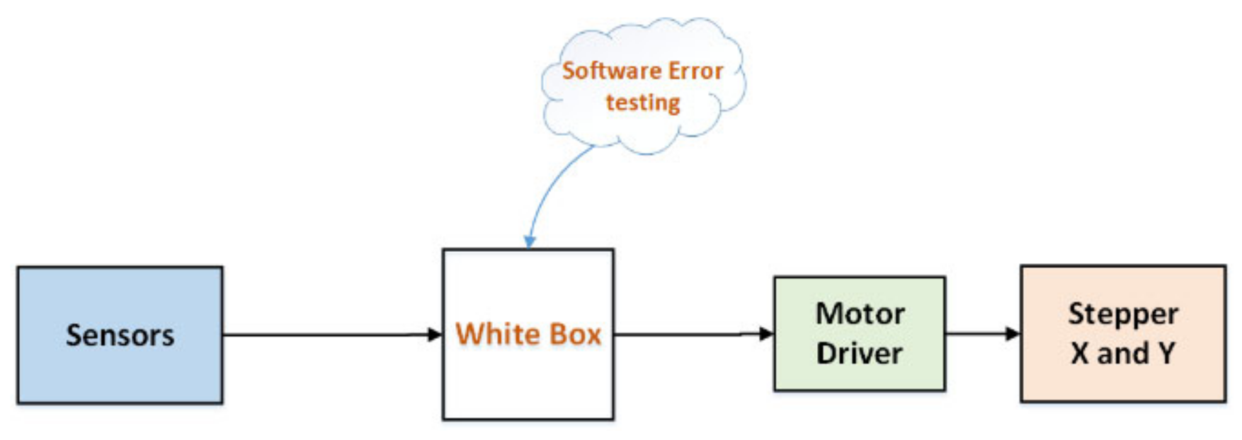
The work in [17] presents a WBST method that sends virtual sensor data from a dedicated cloud platform to a solar tracking device to verify its functionality. The communication channel is an essential component of the WBST as it connects the local hardware to the server via Wi-Fi industrial scientific and medical (ISM) band. By using an ESP 8266 Wi-Fi module as a middle man between the cloud layer and the Arduino UNO microcontroller, the test engineer is capable of transferring massive amounts of data at a given baud rate in order to detect control flow, communication, calculation, and error handling errors. In this paper, the cloud communication and Wi-Fi module from the WBST setup are eliminated and thus a more simplified testing model is obtained, as can be seen in Figure 2.

Accordingly, by modifying several parts of the firmware, zero probability of communication errors was obtained, as well as an improved fault coverage of control flow, calculation, and error handling errors. The improved fault coverage for the offline WBST routines can be seen in

Table 1. Improved fault coverage results for offline WBST.

Test Cases		Error Types				Coverage (%)	Execution Time (minutes)
Test	Total	Control Flow	Communication	Calculation	Error Handling
TP1	840	251	0	85	350	81.66	80
TP2	580	98	0	55	241	71.63	55
TP3	708	185	0	98	211	69.77	64
TP4	736	422	0	43	198	90.08	76

, where error types columns represent the number of detected software errors.

At this point, the unified metrics system that was developed in Section 3 can be applied by discarding the hardware and in-circuit parameters from each of the equations. By doing this, Expression (11) is obtained:

$$\left\{\begin{array}{l}ST{F}_H=0\\ ST{F}_I=0\\ ST{F}_M=\frac{0+ST{F}_S+0}{1}=ST{F}_S\\ ST{F}_M=\frac{0+\frac{E}{T_P\cdot 2^B}+0}{1}=\frac{E_S}{T_P\cdot 2^B}\end{array}\right.$$

(11)

Following, the metrics set will be computed only for the software STF parameter, as presented in the equation set:

$$\left\{\begin{array}{l}ST{F}_{M1}=ST{F}_{S1}\\ ST{F}_{M2}=ST{F}_{S2}\\ ST{F}_{M3}=ST{F}_{S3}\\ ST{F}_{M4}=ST{F}_{S4}\\ ST{F}_{M1}=\frac{E_1}{T_P\cdot 2^B}=\frac{686}{840\cdot 2^5}=\frac{686}{840\cdot 32}=0.0255\\ ST{F}_{M2}=\frac{E_2}{T_P\cdot 2^B}=\frac{394}{580\cdot 2^5}=\frac{394}{580\cdot 32}=0.0212\\ ST{F}_{M3}=\frac{E_3}{T_P\cdot 2^B}=\frac{494}{708\cdot 2^5}=\frac{494}{708\cdot 32}=0.0218\\ ST{F}_{M4}=\frac{E_4}{T_P\cdot 2^B}=\frac{663}{736\cdot 2^5}=\frac{494}{736\cdot 32}=0.0281\end{array}\right.$$

(12)

The previously determined values are calculated for an error factor E extracted from the lines TP1, TP2, TP3, and TP4 found in Table 1 and a constant number B = 5 breakpoints given by the software algorithm of the WBST method. In addition, the total number of test patterns T_P is derived from column 2 of Table 1.

Finally, since the SRF will have the hardware and in-circuit parameters discarded from the unified metrics system, similarly to Expression (11), a simplified equation set will be obtained, as presented:

$$\left\{\begin{array}{l}SR{F}_{M1}=SR{F}_{S1}\\ SR{F}_{M2}=SR{F}_{S2}\\ SR{F}_{M3}=SR{F}_{S3}\\ SR{F}_{M4}=SR{F}_{S4}\\ SR{F}_{M1}=e^{-ST{F}_{S1}}=e^{-0.0255}=0.9748\\ SR{F}_{M2}=e^{-ST{F}_{S2}}=e^{-0.0212}=0.9790\\ SR{F}_{M3}=e^{-ST{F}_{S3}}=e^{-0.0218}=0.9784\\ SR{F}_{M4}=e^{-ST{F}_{S4}}=e^{-0.0281}=0.9722\end{array}\right.$$

(13)

Here, it can be seen that the average value of the SRF parameter is 0.9761, representing the solar tracking system’s reliability when considering software-oriented errors.

4.2. Online Built-In Self-Test Architecture

The built-in self-test (BIST) routines are hardware checking methods that allow the test engineer to deploy a test pattern generator (TPG) and output response analyzer (ORA) in order to verify the functionality of a circuit under test (CUT), which can be a digital device or a chain of electrical circuits.

The work in [18] presents an OBIST architecture that injects random test patterns from a 16-bit linear feedback shift register (LFSR) into a circuit chain composed of an Optocoupler LTV847, Arduino UNO MCU, and two L298N motor drivers in order to obtain a signature database of fully functional and faulty components. The polynomial function, which in our case is given by the expression $P\left(x\right)=1+x+x^3+x^{12}+x^{16}$, is an essential element of the BIST architecture since it allows us to control the amount of patterns that are generated, thus maximizing the number of test vectors that can be injected in the CUTs. For the implementation of the OBIST, in order to be able to construct the hardware-based LFSR, four 74HC194 ICs are required, which are 4-bit bidirectional shift registers. Similarly, for the multiple input signature register (MISR), the same amount of ICs can be used in order to construct two signature databases that are analyzed for error detection, as can be seen in Figure 3.

Since the fault coverage obtained in [18] was efficient, no OBIST hardware implementation parts were necessary to be modified. Thus, the unified metrics system can be adapted to the relations from [16], as expressed in the equation set:

$$\left\{\begin{array}{l}ST{F}_H=\frac{E}{2^D\cdot (2^D-1)}\\ T_P=2^D-1\\ ST{F}_{H1}=\frac{E_1}{2^D\cdot (2^D-1)}\\ ST{F}_{H2}=\frac{E_2}{2^D\cdot (2^D-1)}\\ ST{F}_{H3}=\frac{E_3}{2^D\cdot (2^D-1)}\\ ST{F}_{H4}=\frac{E_4}{2^D\cdot (2^D-1)}\\ ST{F}_{H5}=\frac{E_5}{2^D\cdot (2^D-1)}\end{array}\right.$$

(14)

By replacing the values from Equation (14), the results are obtained, presented in the equation system:

$$\left\{\begin{array}{l}ST{F}_H=\frac{E}{2^{16}\cdot (2^{16}-1)}\\ T_P=2^{16}-1\\ ST{F}_{H1}=\frac{61,570\cdot 65,535}{2^{16}\cdot (2^{16}-1)}=\frac{61,570}{65,534}=0.9395\\ ST{F}_{H2}=\frac{61,557\cdot 65,535}{2^{16}\cdot (2^{16}-1)}=\frac{61,557}{65,534}=0.9393\\ ST{F}_{H3}=\frac{61,550\cdot 65,535}{2^{16}\cdot (2^{16}-1)}=\frac{61,550}{65,534}=0.9392\\ ST{F}_{H4}=\frac{61,554\cdot 65,535}{2^{16}\cdot (2^{16}-1)}=\frac{61,544}{65,534}=0.9391\\ ST{F}_{H5}=\frac{61,563\cdot 65,535}{2^{16}\cdot (2^{16}-1)}=\frac{61,563}{65,534}=0.9394\end{array}\right.$$

(15)

After computing Equation (15), the SRF relations were determined according to the equation system:

$$\left\{\begin{array}{l}SR{F}_H=e^{-ST{F}_H}=\frac{1}{e^{ST{F}_H}}\\ SR{F}_{H1}=e^{-ST{F}_{H1}}=\frac{1}{e^{ST{F}_{H1}}}=0.3919\\ SR{F}_{H2}=e^{-ST{F}_{H2}}=\frac{1}{e^{ST{F}_{H2}}}=0.3920\\ SR{F}_{H3}=e^{-ST{F}_{H3}}=\frac{1}{e^{ST{F}_{H3}}}=0.3920\\ SR{F}_{H4}=e^{-ST{F}_{H4}}=\frac{1}{e^{ST{F}_{H4}}}=0.3921\\ SR{F}_{H5}=e^{-ST{F}_{H5}}=\frac{1}{e^{ST{F}_{H5}}}=0.3919\end{array}\right.$$

(16)

A more general observation is that the level of detail for each graphical representation can be controlled via a granularity factor which is later described in this paper.

4.3. Hybrid Testing Method Based on Boundary Scan and In-Circuit Testing

Hybrid testing methods are a type of mixed testing routines that allow the test engineer to combine two or more testing techniques in order to cover multiple categories of errors and faults. The work in [19] presents a hybrid testing approach composed of an FPICT device and JTAG boundary scan test technologies. The FPICT is used for testing the physical parameter values of our dual-axis solar tracking equipment comprising 1× Optocoupler, 1× Arduino UNO board, and 2× L298N motor drivers. Due to the lack of existing JTAG testing facilities on the Arduino UNO board, it was replaced with an STM32 development board. To gain access to the internal logic of the STM32 microcontroller, the dedicated and low-cost ST-Link V2 JTAG adapter was tethered to the FPICT unit. To make all five CUTs test points (TPs) more available to the FPICT system, a custom modular printed circuit board (PCB) was built.

For computing the fault coverage of the syntax errors, as well as of the structural and stuck-at-faults presented in

Table 2. Experimental results regarding our JTAG boundary scan and flying probe in-circuit tester (FPICT) procedure [19].

Test Schedule				Fault Coverage (%)
No. of Days		No. of Test Cases Per Day		Error Types
		8:00 a.m.	4:00 p.m.	Syntax Errors	Structural Faults	Stuck-at-Faults
Mostly Sunny Week	1	1	1	70.20	78.20	60.10
	2			69.10	77.10	65.10
	3			65.14	65.20	69.15
	4			67.20	66.20	56.10
	5			66.66	60.20	55.45
	6			71.13	79.90	59.10
	7			65.20	75.13	52.01
Partly Cloudy Week	1	1	1	69.65	77.65	62.55
	2			67.67	71.70	64.62
	3			68.70	72.70	58.10
	4			68.43	72.20	57.27
	5			70.66	69.20	64.12
	6			67.70	71.65	54.10
	7			71.16	66.20	57.30
Total		28		Average Fault Coverage
				67.80	71.70	59.57

, an automated Python script was used that triggers the JTAG boundary scan testing method at scheduled times (in our case, at 8:00 a.m. and 4:00 p.m.) and which can be manually configured by the user.

Due to the effective combination of JTAG and FPICT testing technologies, a balanced fault coverage of software, hardware, and in-circuit errors was accomplished. With the experimental data provided in Table 2, the unified metrics system for mixed test scenarios can be computed.

First, regarding the mostly sunny week, according to Equation (9), the equation set for the STF parameter is calculated as expressed in Equation (17):

$$\left\{\begin{array}{l}ST{F}_M=\frac{ST{F}_H+ST{F}_S+ST{F}_I}{3}\\ ST{F}_M=\frac{\frac{E_H}{2^D\cdot (2^D-1)}+\frac{E_S}{T_P\cdot 2^B}+\frac{E_I}{N_R\cdot 2^P}}{3}\\ ST{F}_{M1}=\frac{\frac{E_{H1}}{2^D\cdot (2^D-1)}+\frac{E_{S1}}{T_P\cdot 2^B}+\frac{E_{I1}}{N_R\cdot 2^P}}{3}\\ ST{F}_{M2}=\frac{\frac{E_{H2}}{2^D\cdot (2^D-1)}+\frac{E_{S2}}{T_P\cdot 2^B}+\frac{E_{I2}}{N_R\cdot 2^P}}{3}\\ ST{F}_{M3}=\frac{\frac{E_{H3}}{2^D\cdot (2^D-1)}+\frac{E_{S3}}{T_P\cdot 2^B}+\frac{E_{I3}}{N_R\cdot 2^P}}{3}\\ ST{F}_{M4}=\frac{\frac{E_{H4}}{2^D\cdot (2^D-1)}+\frac{E_{S4}}{T_P\cdot 2^B}+\frac{E_{I4}}{N_R\cdot 2^P}}{3}\\ ST{F}_{M5}=\frac{\frac{E_{H5}}{2^D\cdot (2^D-1)}+\frac{E_{S5}}{T_P\cdot 2^B}+\frac{E_{I5}}{N_R\cdot 2^P}}{3}\\ ST{F}_{M6}=\frac{\frac{E_{H6}}{2^D\cdot (2^D-1)}+\frac{E_{S6}}{T_P\cdot 2^B}+\frac{E_{I6}}{N_R\cdot 2^P}}{3}\\ ST{F}_{M7}=\frac{\frac{E_{H7}}{2^D\cdot (2^D-1)}+\frac{E_{S7}}{T_P\cdot 2^B}+\frac{E_{I7}}{N_R\cdot 2^P}}{3}\end{array}\right.$$

(17)

The above metrics system is calculated for a number of D = 16 flip-flops (for stuck-at-faults), T_{P =} 840 (for syntax errors), and N_R = 1000 (for structural faults). Accordantly, the following results are obtained, presented in Equation (18):

$$\left\{\begin{array}{l}ST{F}_{M1}=\frac{0.6010+0.0219+0.391}{3}=\frac{1.0139}{3}=0.33796\\ ST{F}_{M2}=\frac{0.6510+0.0215+0.3855}{3}=\frac{1.058}{3}=0.3526\\ ST{F}_{M3}=\frac{0.6915+0.0203+0.326}{3}=\frac{1.0378}{3}=0.34593\\ ST{F}_{M4}=\frac{0.5610+0.021+0.331}{3}=\frac{0.913}{3}=0.3043\\ ST{F}_{M5}=\frac{0.5545+0.020+0.301}{3}=\frac{0.8755}{3}=0.2918\\ ST{F}_{M6}=\frac{0.5910+0.022+0.3756}{3}=\frac{0.9886}{3}=0.2918\\ ST{F}_{M7}=\frac{0.5201+0.020+0.3755}{3}=\frac{0.9156}{3}=0.3052\end{array}\right.$$

(18)

Secondly, based on the results obtained in the equation set (18), the global SRF parameter is computed, as presented in Equation (19):

$$\left\{\begin{array}{l}SR{F}_M=\frac{SR{F}_H+SR{F}_S+SR{F}_I}{3}\\ SR{F}_M=\frac{\exp [\frac{E}{2^D\cdot (2^D-1)}]+\exp [\frac{E}{T_P\cdot 2^B}]+\exp [\frac{E}{N_R\cdot 2^P}]}{3}\\ SR{F}_{M1}=\frac{e^{-ST{F}_{H1}}+e^{-ST{F}_{S1}}+e^{-ST{F}_{I1}}}{3}\\ SR{F}_{M2}=\frac{e^{-ST{F}_{H2}}+e^{-ST{F}_{S2}}+e^{-ST{F}_{I2}}}{3}\\ SR{F}_{M3}=\frac{e^{-ST{F}_{H3}}+e^{-ST{F}_{S3}}+e^{-ST{F}_{I3}}}{3}\\ SR{F}_{M4}=\frac{e^{-ST{F}_{H4}}+e^{-ST{F}_{S4}}+e^{-ST{F}_{I4}}}{3}\\ SR{F}_{M5}=\frac{e^{-ST{F}_{H5}}+e^{-ST{F}_{S5}}+e^{-ST{F}_{I5}}}{3}\\ SR{F}_{M6}=\frac{e^{-ST{F}_{H6}}+e^{-ST{F}_{S6}}+e^{-ST{F}_{I6}}}{3}\\ SR{F}_{M7}=\frac{e^{-ST{F}_{H7}}+e^{-ST{F}_{S7}}+e^{-ST{F}_{I7}}}{3}\end{array}\right.$$

(19)

After solving the metrics system, Equation (19), the SRF parameters are obtained, as presented in the equation set:

$$\left\{\begin{array}{l}SR{F}_{M1}=\frac{0.5482+0.9783+0.6763}{3}=0.7342\\ SR{F}_{M2}=\frac{0.5215+0.9787+0.6801}{3}=0.7267\\ SR{F}_{M3}=\frac{0.5008+0.9799+0.7218}{3}=0.7341\\ SR{F}_{M4}=\frac{0.5706+0.9792+0.7182}{3}=0.756\\ SR{F}_{M5}=\frac{0.5743+0.9801+0.7400}{3}=0.7648\\ SR{F}_{M6}=\frac{0.5537+0.9782+0.6868}{3}=0.7395\\ SR{F}_{M7}=\frac{0.5944+0.9801+0.6869}{3}=0.7538\end{array}\right.$$

(20)

Similarly, the mixed test scenarios for the partially cloudy week are evaluated with the equation system presented in Equation (21):

$$\left\{\begin{array}{l}ST{F}_M=\frac{ST{F}_H+ST{F}_S+ST{F}_I}{3}\\ ST{F}_M=\frac{\frac{E_H}{2^D\cdot (2^D-1)}+\frac{E_S}{T_P\cdot 2^B}+\frac{E_I}{N_R\cdot 2^P}}{3}\\ ST{F}_{M8}=\frac{\frac{E_{H8}}{2^D\cdot (2^D-1)}+\frac{E_{S8}}{T_P\cdot 2^B}+\frac{E_{I8}}{N_R\cdot 2^P}}{3}\\ ST{F}_{M9}=\frac{\frac{E_{H9}}{2^D\cdot (2^D-1)}+\frac{E_{S9}}{T_P\cdot 2^B}+\frac{E_{I9}}{N_R\cdot 2^P}}{3}\\ ST{F}_{M10}=\frac{\frac{E_{H10}}{2^D\cdot (2^D-1)}+\frac{E_{S10}}{T_P\cdot 2^B}+\frac{E_{I10}}{N_R\cdot 2^P}}{3}\\ ST{F}_{M11}=\frac{\frac{E_{H11}}{2^D\cdot (2^D-1)}+\frac{E_{S11}}{T_P\cdot 2^B}+\frac{E_{I11}}{N_R\cdot 2^P}}{3}\\ ST{F}_{M12}=\frac{\frac{E_{H12}}{2^D\cdot (2^D-1)}+\frac{E_{S12}}{T_P\cdot 2^B}+\frac{E_{I12}}{N_R\cdot 2^P}}{3}\\ ST{F}_{M13}=\frac{\frac{E_{H13}}{2^D\cdot (2^D-1)}+\frac{E_{S13}}{T_P\cdot 2^B}+\frac{E_{I13}}{N_R\cdot 2^P}}{3}\\ ST{F}_{M14}=\frac{\frac{E_{H14}}{2^D\cdot (2^D-1)}+\frac{E_{S14}}{T_P\cdot 2^B}+\frac{E_{I14}}{N_R\cdot 2^P}}{3}\end{array}\right.$$

(21)

The STF parameters for the partially cloudy week are determined for a number D = 16 flip-flops, T_P = 840 software test vectors, N_R = 1000 in-circuit routines, according to the equation set:

$$\left\{\begin{array}{l}ST{F}_{M8}=\frac{0.6255+0.0217+0.3882}{3}=0.3451\\ ST{F}_{M9}=\frac{0.6462+0.0211+0.3585}{3}=0.3419\\ ST{F}_{M10}=\frac{0.5810+0.0214+0.3635}{3}=0.3219\\ ST{F}_{M11}=\frac{0.5727+0.0213+0.361}{3}=0.3183\\ ST{F}_{M12}=\frac{0.5727+0.0228+0.346}{3}=0.3364\\ ST{F}_{M13}=\frac{0.5410+0.0211+0.358}{3}=0.3068\\ ST{F}_{M14}=\frac{0.5730+0.022+0.331}{3}=0.3087\end{array}\right.$$

(22)

Similarly, the unified metrics set for the SRF parameter are calculated according to the general equation system:

$$\left\{\begin{array}{l}SR{F}_M=\frac{SR{F}_H+SR{F}_S+SR{F}_I}{3}\\ SR{F}_M=\frac{\exp [\frac{E}{2^D\cdot (2^D-1)}]+\exp [\frac{E}{T_P\cdot 2^B}]+\exp [\frac{E}{N_R\cdot 2^P}]}{3}\\ SR{F}_{M8}=\frac{e^{-ST{F}_{H8}}+e^{-ST{F}_{S8}}+e^{-ST{F}_{I8}}}{3}\\ SR{F}_{M9}=\frac{e^{-ST{F}_{H9}}+e^{-ST{F}_{S9}}+e^{-ST{F}_{I9}}}{3}\\ SR{F}_{M10}=\frac{e^{-ST{F}_{H10}}+e^{-ST{F}_{S10}}+e^{-ST{F}_{I10}}}{3}\\ SR{F}_{M11}=\frac{e^{-ST{F}_{H11}}+e^{-ST{F}_{S11}}+e^{-ST{F}_{I11}}}{3}\\ SR{F}_{M12}=\frac{e^{-ST{F}_{H12}}+e^{-ST{F}_{S12}}+e^{-ST{F}_{I12}}}{3}\\ SR{F}_{M13}=\frac{e^{-ST{F}_{H13}}+e^{-ST{F}_{S13}}+e^{-ST{F}_{I13}}}{3}\\ SR{F}_{M14}=\frac{e^{-ST{F}_{H14}}+e^{-ST{F}_{S14}}+e^{-ST{F}_{I14}}}{3}\end{array}\right.$$

(23)

Thus, after substituting all STF values from the previously computed equation system, the remaining SRF parameters are obtained in the equation set:

$$\left\{\begin{array}{l}SR{F}_{M8}=\frac{0.5349+0.9784+0.6782}{3}=0.7305\\ SR{F}_{M9}=\frac{0.5240+0.9790+0.6987}{3}=0.7339\\ SR{F}_{M10}=\frac{0.5593+0.9787+0.6952}{3}=0.7444\\ SR{F}_{M11}=\frac{0.5639+0.9781+0.7075}{3}=0.7374\\ SR{F}_{M12}=\frac{0.5266+0.9801+0.7400}{3}=0.7648\\ SR{F}_{M13}=\frac{0.5821+0.9790+0.6988}{3}=0.7533\\ SR{F}_{M14}=\frac{0.5638+0.9780+0.7182}{3}=0.7533\end{array}\right.$$

(24)

Finally, by analyzing the average values from Table 2, the global STF and SRF parameters can be accurately computed according to the metrics system:

$$\left\{\begin{array}{l}ST{F}_M=\frac{ST{F}_H+ST{F}_S+ST{F}_I}{3}\\ ST{F}_M=\frac{\frac{N_E\cdot T_V}{T_P\cdot 2^D}+\frac{N_E\cdot T_V}{T_P\cdot 2^B}+\frac{N_E\cdot T_R}{N_R\cdot 2^P}}{3}\\ SR{F}_M=\frac{SR{F}_H+SR{F}_S+SR{F}_I}{3}\\ SR{F}_M=\frac{\exp [\frac{N_E\cdot T_V}{T_P\cdot 2^D}]+\exp [\frac{N_E\cdot T_V}{T_P\cdot 2^B}]+\exp [\frac{N_E\cdot T_V}{T_P\cdot 2^P}]}{3}\end{array}\right.$$

(25)

Therefore, by replacing each of the variables in Equation (25), the reliability factor of our solar tracking system is obtained over two weeks, as computed in the equation set:

$$\left\{\begin{array}{l}ST{F}_M=\frac{0.5957+0.0211+0.358}{3}=0.3251\\ SR{F}_M=\frac{0.5511+0.9790+0.6987}{3}=0.7429\end{array}\right.$$

(26)

According to the last equation set (Equation (26)), it is observable that the global SRF of the entire solar tracking device is rated at 74.29%.

5. Experimental Setup and Results

This section presents a detailed overview of the experimental setup encompassing the combined testing suite and a smart scheduling diagram, as well as the graphical generated results obtained from the previously calculated unified metrics systems.

5.1. Proposed Combined Testing Suite for Improving the Solar Reliability Factor

One of the primary goals of this paper is to fuse various testing methodologies into one compact design composed of software, hardware, and ICT techniques to extend the SRF parameter of solar tracking devices.

The interface of our virtual environment, as can be observed in Figure 4, is divided into two parts: software and hardware interface.

The software interface contains the algorithm implementations of the WBST, OBIST, FPICT, and JTAG methods and is directly connected to the analysis block. The hardware interface, on the other hand, is placed outside the software layer and uses a TPG unit (hardware-based LFSR) for injecting test patterns into the OBIST block and an ORA unit (hardware-based MISR) for collecting the results from the signature-based testing technique and further directing them to the analysis block. The detailed reports created inside the analysis block are displayed on the central console (in our case, a Raspberry Pi 3B+ platform) after each combined test ends its daily cycle.

It is worth mentioning that the proposed combined testing suite achieves self-sufficiency regarding energy needs for the proposed hybrid testing method and the entire solar tracking equipment by making use entirely of solar energy. The entire testing suite consumes between 5 Wh and 6.13 Wh during its operational status [19], while the energy generation provided by the mobile solar panel compensates for the power usage in both, mostly sunny (10.76 Wh) and partly cloudy (5.51 Wh) day scenarios. The low power consumption of our experimental setup was made possible by employing an intelligent triggering mechanism for each testing routine which is based on a smart scheduling diagram described in the next subchapter of this paper.

5.2. Smart Scheduling Diagram for the Proposed Combined Testing Suite

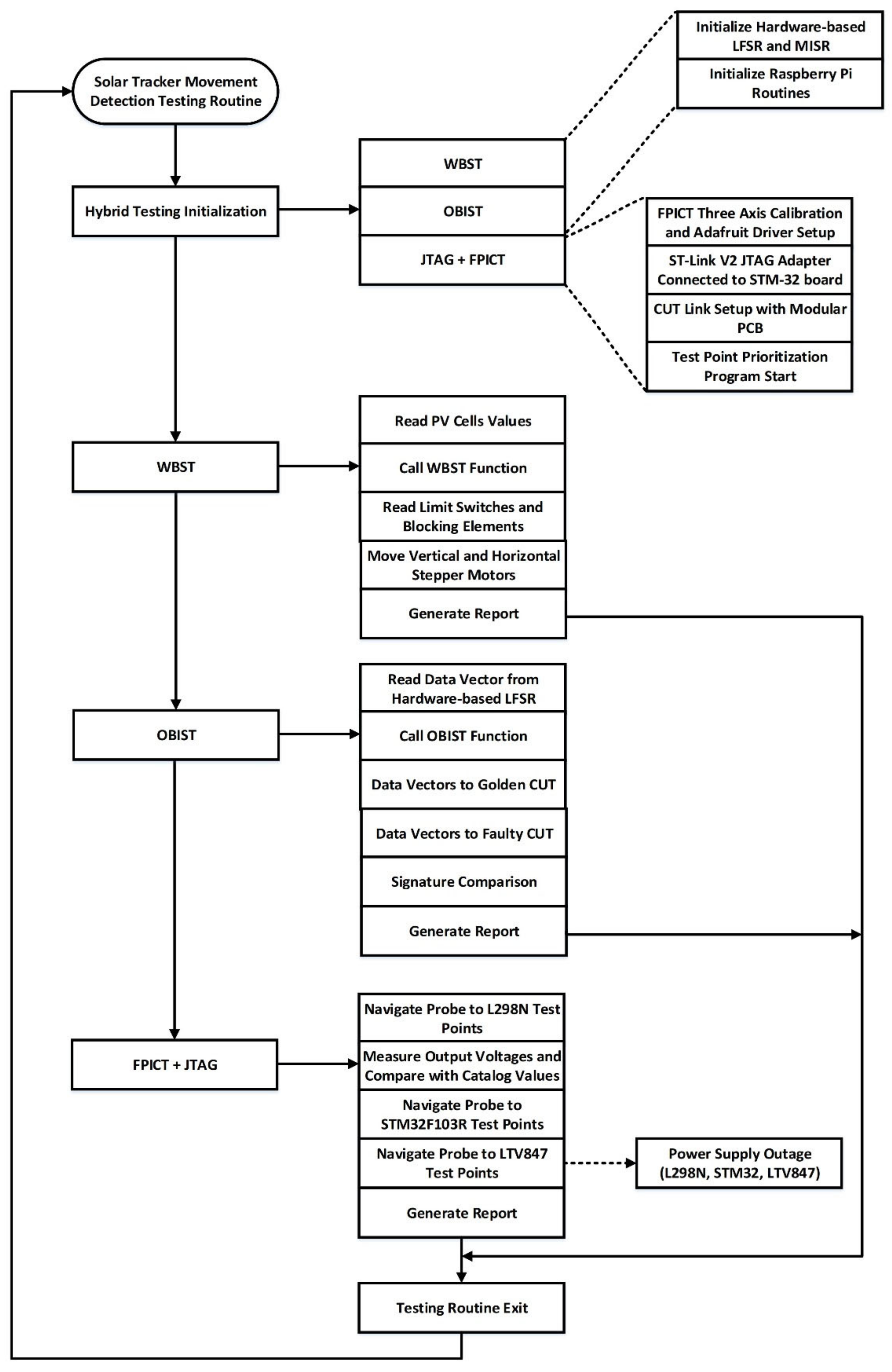
The proposed combined testing suite executes each testing routine according to an automated scheduling diagram that considers solar panel movement a vital element of the triggering mechanism. As shown in Figure 5, the combined testing suite is scheduled to launch when the solar tracker movement is detected by an automated script that runs in the Python programming environment.

In the first stage of the scheduling program, the hybrid testing initialization will prioritize the WBST and OBIST routines, which also involves the configuration of the hardware-based LSFR and MSIR with their initial seed values, as well as the generic Raspberry Pi 3B+ routines configuration. The FPICT and JTAG program schedule, being a mixed testing routine, consists of the three-axis calibration and modular PCB connection with the STM32 board (for the ICT), as well as the ST-Link tethering to the STM32 board (for the boundary scan procedure).

The second stage of the scheduling program refers strictly to the WBST routines and the actions that the test program will take to check the Arduino UNO MCU for software errors. Since the cloud layer from the WBST setup was eliminated, the test program will read the PV cells’ voltage values directly from the solar panel. At this point, the test program will call the WBST function and will verify the algorithm mechanism in a continuous loop while monitoring and reading the Boolean values received from the limit switches and blocking elements. If no software errors were detected at this stage, the solar tracker would move the vertical and horizontal motors until it reaches its optimum position. In the opposite scenario, a detailed report with the software error types will be generated by the test program.

The third stage of the scheduling program will trigger the OBIST routine that will initially read the data vector provided by the hardware-based LFSR unit. Once the first test pattern is loaded, the test program will immediately call the OBIST primary function that will inject test vectors into the golden and faulty CUTs to gather their responses in the MISR unit. Through signature comparison, the test program will decide which signatures in the database are faulty and will accordantly generate a report with the hardware faults.

The fourth stage of the smart scheduling diagram refers to the FPICT and JTAG methods, focusing on the ICT component. During the last testing phase, the custom-built FPICT will navigate the probe to the L298N TPs to measure the output voltages and compare them with the catalog values. Similarly, the FPICT device will measure the voltage values from the STM32 development board and LTV847 Optocoupler to check for power supply outages. If any structural faults are detected successfully at the IC-level design, a detailed report will be generated and sent together with the previous reports to the central console for future analyses.

5.3. Graphical Representations of the Global STF and SRF Parameters

Accelerated testing [4] is an essential and indispensable quality assessment tool for checking automated PV systems for long-term usage, which allows us to inject a large amount of software, hardware, and in-circuit errors into the system through simulation. When compared to real-time testing, accelerated testing has several advantages, enumerated as follows: (a) is a non-intrusive method, meaning that it does not impact the performance of the system and also circumvents unnecessary damage to the components; (b) simulates software, hardware, and in-circuit errors in a short time (a couple of hours or days) in opposition with real-time test scenarios (which can take months or even years); (c) uses a minimum amount of resources and is considered a low-cost solution on the PV market.

In this paper, by using the experimental data obtained from our accelerated hybrid testing solution, the global STF and SRF parameters were determined over a two-week period.

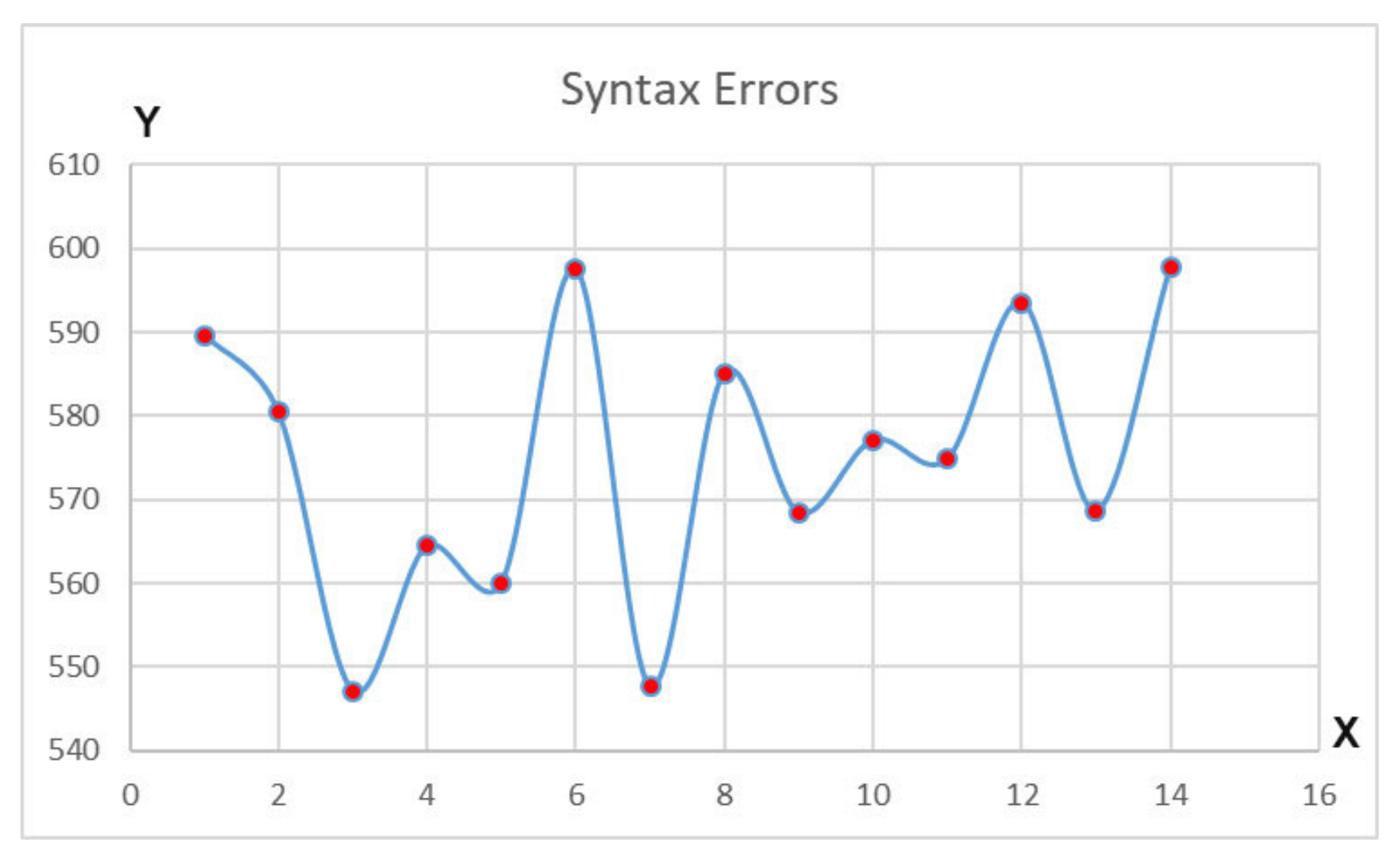
First, the graphical representations of the syntax errors will be generated, as depicted in Figure 6.

To represent the test factor for syntax errors, it is crucial to define the STF parameter’s dependability concerning the error factor E. As shown in Figure 6, an average value of E = 569 software errors was detected during the two weeks test time. The corresponding graphical representations of the STF (a) and SRF (b) parameters can be seen in Figure 7.

Concerning Figure 6 and Figure 7a, since the test factor is computed with the help of the fault coverage, it can be immediately noticed that the graphical representations of the software error factor E and STF parameter are identical. Based on these findings, the remaining graphical charts of the hardware and in-circuit STF and SRF parameters will be generated.

Secondly, the hardware STF (a) and SRF (b) were calculated for an average value of E = 39,039 stuck-at-faults, and their graphical distributions over two weeks are depicted in Figure 8.

Thirdly, the in-circuit STF (a) and SRF (b) were computed for an average value of E = 717 structural faults, and their graphical distribution models can be seen in Figure 9.

At this point, it is essential to mention that all graphical representations were created individually for each testing method, based on the generated reports (see Figure 5). However, since a unified metrics system was applied, the results obtained in each equation set can be used for mixed test scenarios computation. According to Equations (18), (20), (22), and (24), the graphical representation of the global STF (a) and SRF (b) is illustrated in Figure 10.

Finally, as can be seen in

Table 3. Comparison between the fault coverage-aware metrics, proposed unified metrics system and Weibull distribution model regarding calculation steps and execution time [20]; adapted from [16].

Crt. Nr.	Fault Coverage Aware Metrics	Proposed Unified Metrics System	Weibull Distribution Model	Runtime Execution
				Fault Coverage-Aware Metrics [16]		Unified Metrics System		Weibull Distribution [20]
				Speed (ms)	Steps (n)	Speed (ms)	Steps (n)	Speed (ms)	Steps (n)
1	Metrics Execution Cycles	Unified Metrics Execution Cycles	Weibull Execution Cycles	0.03	69	0.03	76	0.1	274
2				0.02	69	0.02	76	0.1	274
3				0.02	69	0.02	76	0.09	274
4				0.02	69	0.02	76	0.09	274
5				0.02	69	0.02	76	0.08	274
6				0.02	69	0.02	76	0.08	274
7				0.02	69	0.02	76	0.09	274
8				0.02	69	0.02	76	0.08	274
Average Values				0.02125	69	0.02125	76	0.08875	274

, this paper presents a comparison between the proposed unified metrics system, our earlier fault coverage-aware metrics [16], and the Weibull distribution model [20] regarding calculation steps and execution time (measured in milliseconds).

This comparison was realized using the Python programming environment. It can be observed that the unified metrics system only adds seven additional steps over the original fault coverage-aware metrics, translating into a 9.21% loss while maintaining the same speed of cycle execution. Consequently, it can be seen that the proposed unified metrics system significantly reduces the computation time by 85.91% and the number of calculation steps by 72.26%, showing that our metrics are considerably more efficient when compared to the standard Weibull distribution model.

6. Conclusions

This paper presents a novel unified metrics system based on a fault coverage-aware metrics set that calculates an STF and SRF parameter for assessing the reliability of a dual-axis solar tracking device. By using a combined testing suite composed of software, hardware, and ICT methods, this paper aims to improve the SRF parameter and thus adapt the fault coverage-aware metrics for mixed test scenarios. By employing a unified metrics system, the main goal was to increase the fault domain to multiple error types which can affect the performance of solar tracking devices, and thus impact the global SRF parameter. Additionally, it was demonstrated that accelerated testing is a superior tool for assessing the reliability of solar tracking systems when compared to real-time testing, where different error types occur rarely and the test time is considerably increased. Finally, four energy-efficient testing techniques encompassing WBST, OBIST, FPICT, and JTAG methods were fused into one compact and low-cost testing design which makes use entirely of solar energy during operation. The experimental results show that our proposed unified metrics system is efficient in terms of runtime execution, reducing the computation time by 85.91% and the number of calculation steps by 72.26%, compared to the standard Weibull distribution model. Although our unified metrics system improves the reliability analysis of solar tracking systems, it fails to increase the value of the SRF parameter. In future work, we plan to reduce the fault coverage of multiple types of errors that were studied in this paper in order to increase the SRF parameter which characterizes the functionality of the tested solar tracking system.