Entropy Rates and Efficiency of Convecting-Radiating Fins ^†

Abstract

We present a novel indicator for the effectiveness of longitudinal, convecting-radiating fins to dissipate heat. Starting from an analysis of the properties of the entropy rate of the steady state, we show how it is possible to assess the efficiency of such devices by looking at the amount of entropy produced in the heat transfer process. Our study concerns both purely convective fins and convection-radiant fins and takes advantage of explicit expressions for the distribution of heat along the fin. It is shown that, in a suitable limit, the standard definition of efficiency and the entropic definition coincide. The role of the fluid temperature is explicit in the new definition and in the purely convective case. An application to an aluminium fin is given. Analytical and numerical results are discussed.

1. Introduction

Longitudinal fins are widely adopted devices used to enhance heat dissipation from a given surface (see e.g., [1,2] and the references therein). The mechanisms of exchange of the thermal energy in heat sink devices can be conduction, convection, or radiation [1]. The description of these three mechanisms depends on the physical hypothesis assumed, and the mathematical models reflect the corresponding assumptions. For conduction and convection, by assuming that Fourier’s and Newton’s laws hold, the corresponding models of temperature distribution along the fin are linear. For particular applications or materials, these basic models can be dressed with further assumptions, usually giving some drawbacks: for example, if the dependence of thermal conductivity on temperature cannot be neglected, Fourier’s law changes from linear to nonlinear and it becomes challenging to obtain analytical results [3]. Furthermore, if the effects of radiation are considered, an additional term appears in the equations and the corresponding thermodynamic model becomes intrinsically nonlinear [1,2]. By intrinsically, we mean that, even assuming that all the thermal coefficients are independent of temperature, the underlying equations are nonlinear. The geometry of the fins is another key factor to take into account at the design level: rectangular, triangular, or cylindrical fins are only some of the most common shapes considered in the literature, and different shapes may be suitable for specific applications.

The problem of evaluation of the efficiency of a convecting-radiating longitudinal fin with an arbitrary profile has been considered in [4], where it has been shown how it is possible to obtain explicitly the temperature of the steady state in convecting-radiating fins. The value of the efficiency, i.e., the ratio of actual heat transfer to ideal heat transfer for a fin of infinite thermal conductivity, was determined by many variables that include boundary conditions, specific values of thermal coefficients, the specific function profile of the fin, and the temperatures of the environment and of the base of the fin. The simplest configuration is that of a rectangular fin without radiation losses, with fixed temperature at the base, and with an insulated tip. The corresponding efficiency $\eta$ in this case is given by the well-known Gardner’s formula $\eta =\frac{tanh\left(m\right)}{m}$, where m is a dimensionless parameter depending on the square root of the ratio between the fin heat transfer coefficient and the thermal conductivity. We observe that Gardner’s result is independent of the temperature gradient between the base and the fluid adjacent to the fin: this fact is a consequence of the linearity of the equations for the temperature when the only mechanism of dissipation is the convection. In our opinion, the independence of the efficiency from the temperature of the base of the fin and from the temperature of the fluid is a weak point of the classical formulation of the efficiency, and this idealization is expected to give accurate results only for small values of the difference between the base temperature and the fluid temperature: as the gradient increases, both the values of actual and ideal heat transferred to the environment increase, but their ratio may not result in a constant [5].

In this work, we introduce a novel indicator for the efficiency of the fin by looking at the entropy produced by the fin in its steady state. We consider the entropy produced by the fin in the process of dissipation of heat both by convection and radiation mechanisms. The profile of the fin is not given and, indeed, is another unknown variable in our equations, making our result adaptable to different applications. The nonlinear analysis of the temperature distribution along the fin is based on the results obtained in [4], where a methodology to obtain explicit solutions has been given. The model is one-dimensional, and the fin considered has a plane of symmetry perpendicular to the plane base support. This model is widely adopted in literature (see, e.g., [1,2]) and simple enough to be manipulated analytically. This gives the possibility to obtain, at least in simple cases, explicit fromulae for the efficiency and to make comparisons with the classical results. The pure convective case is analyzed first by showing how the entropy-based efficiency represents a concrete extension of the classical efficiency: indeed, if on the one hand it is possible within the limit of a small temperature gradient to obtain the classic results from our formulas, on the other hand, the temperature difference plays an explicit role and its effect can be evaluated directly. We emphasize that practical issues, such as cost, adequate design considerations, or materials may be specific to a given application and, as such, cannot enter into this study. For these aspects, the interested reader can look for examples in [1,2] and the references therein.

The work is organized as follows: in Section 2, the main equations describing the evolution of the temperature along the fin and the relative boundary conditions are presented. The expression of the entropy rate produced by the convection and radiation by the fin is also introduced. In Section 3, an entropy-based indicator is defined and discussed to measure the effectiveness of the fin in dissipating heat. For definiteness, the application of the method to some relevant cases is illustrated. In Section 4, the formulas previously introduced are applied to the case of a purely convective fin. In particular, the efficiency of a rectangular fin is calculated and a comparison is made with the classical results from the literature. Furthermore, it is shown that, if the difference between the base temperature and the fluid temperature is small, the classical definition and the new definition coincide for an arbitrary profile of the fin. In Section 5, the case of a fin dissipating by convection and radiation is presented. In Section 6, we present a specific application of the formulae obtained to an aluminum fin, with a base at $T=800$ K and a fluid at $T=400$ K. A comparison between the entropic efficiency and the classical efficiency is given. Finally, in the conclusions, we discuss our results and some potential generalizations.

2. The Entropy Rate Due to Heat Exchange

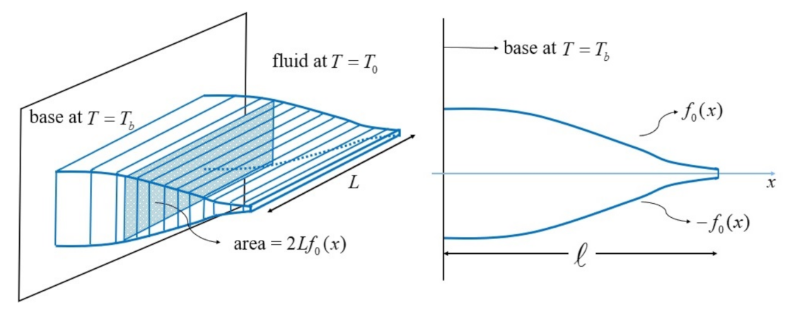
Let us consider a longitudinal fin with an arbitrary profile attached to a base, which is at a temperature $T_b$. The fin length (alongside the base) is L, whereas the fin thickness at a distance x from the base is $2f_0\left(x\right)\ge 0$. We consider a symmetric fin for which the profile is confined by the curves $f_0\left(x\right)$ and $-f_0\left(x\right)$, where x is the coordinate in the direction perpendicular to the fin base (see Figure 1). The half thickness at the base is $f_b=f_0(x=0)$, whereas at the fin tip, located at $x=\ell$, the half thickness is $f_t=f_0\left(\ell \right)$. We assume that Fourier’s law holds within the fin and that the temperature varies only along the x direction. Furthermore, the variation in internal energy is assumed to be equal to energy gains (or losses) by conduction, radiation, and convection.

Let $\kappa$ be the thermal conductivity of the homogeneous material, $\rho$ be its density, $\kappa$ be its thermal conductivity, c be its specific heat, h be the convective heat transfer coefficient, and $\sigma$ be the Stefan–Boltzmann constant. Then, the evolution of the temperature $T(x,t)$ is governed by the following equation [4]:

$$\rho c{f}_0\left(x\right)\frac{\partial T}{\partial t}=\kappa \frac{\partial }{\partial x}\left(f_0\left(x\right)\frac{\partial T}{\partial x}\right)-2h\left(1+2\frac{f_0}{L}\right)(T-T_0)-2\sigma ϵ\left(1+2\frac{f_0}{L}\right)(T^4-T_1^4),$$

(1)

where $T_1$ is the temperature of the effective irradiation environment. Accordingly, $ϵ\sigma T_1^4$ represents the radiant energy absorbed by the fin per unit of time and surface. Additionally, $T_0$ is the temperature of the fluid and $ϵ$ is the emissivity of the fin.

When the thickness of the fin is small compared with respect to its length, the term $f_0/L$ can be ignored, giving

$$\rho c{f}_0\left(x\right)\frac{\partial T}{\partial t}=\kappa \frac{\partial }{\partial x}\left(f_0\left(x\right)\frac{\partial T}{\partial x}\right)-2h(T-T_0)-2\sigma ϵ(T^4-T_1^4).$$

(2)

The above equation describes the transient evolution of the temperature in time along the fin: in the rest of the paper, we look at the steady state, described by the same Equation (2), with the left-hand side equal to zero. Additionally, we assume the fin to be in general non-gray, with $T_1^4=\varphi T_0^4$, where $\varphi$ is the ratio between the absorptivity and the emissivity of the fin [2]. In the case of a gray fin, one has to set $\varphi =1$ [2].

Equation (2) must be supplied with the initial and boundary conditions: according to [4], we assume that the boundary conditions are given by

$$f_0\left(x\right){\left.\frac{dT}{dx}\right|}_{x=0}-{\left.{\eta }_0(T-T_b)\right|}_{x=0}-{\xi }_0{\left.(T^4-\varphi T_b^4)\right|}_{x=0}=0.$$

(3)

and

$$f_0\left(x\right){\left.\frac{dT}{dx}\right|}_{x=\ell }+{\left.{\eta }_1(T-T_0)\right|}_{x=\ell }+{\xi }_1{\left.(T^4-\varphi T_0^4)\right|}_{x=\ell }=0.$$

(4)

where ${\eta }_i$ and ${\xi }_i$, $i=0,1$ denote positive constants proportional to the Biot and radiation-conduction numbers of the ends of the fin, respectively. The initial condition is given by ${\left.T\right|}_{t=0}=T(x,0)=T_{in}\left(x\right)$.

The dimensionless variables $z=x/\ell$ and $\tau =\kappa t/\rho c{\ell }^2$ are introduced for further convenience. Moreover, we define $\theta =T/T_b$, ${\theta }_{in}=T_{in}/T_b$, $\alpha =2h{\ell }^2/\left(f_b\kappa \right)$, $\beta =2\sigma ϵ{\ell }^2{T}_b^3/\left(f_b\kappa \right)$, and $f\left(z\right)=f_0\left(z\ell \right)/f_b$. Equation (2) becomes

$$f\left(z\right)\frac{\partial \theta }{\partial \tau }=\frac{\partial }{\partial z}\left(f\left(z\right)\frac{\partial \theta }{\partial z}\right)-\alpha (\theta -{\theta }_0)-\beta ({\theta }^4-\varphi {\theta }_0^4)$$

(5)

with initial conditions ${\theta (z,\tau )|}_{\tau =0}=\theta (z,0)={\theta }_{in}\left(z\right)$ and boundary conditions

$$\begin{array}{cc}\hfill & {\left.f\left(z\right)\frac{d\theta }{dz}\right|}_{z=0}-{\left.B{i}_0(\theta -1)\right|}_{z=0}-{\left.N_0({\theta }^4-\varphi )\right|}_{z=0}=0,\hfill \\ \hfill & {\left.f\left(z\right)\frac{d\theta }{dz}\right|}_{z=1}+{\left.B{i}_1(\theta -{\theta }_0)\right|}_{z=1}+{\left.N_1({\theta }^4-\varphi {\theta }_0^4)\right|}_{z=1}=0,\hfill \end{array}$$

(6)

where the Biot numbers $B{i}_j={\eta }_j\ell /f_b$, $j=0,1$ and the radiation-conduction numbers $N_j={\xi }_j\ell /f_b$, $j=0,1$ were introduced.

Our system is given by the fin and its base, with the base being a thermal reservoir at temperature $T_b$. The external environment is represented by the fluid at a constant temperature $T_0$. Our aim is to define an entropy-based efficiency by taking into account the irreversibilities of the system alone. For this reason, we consider the entropy rate due to heat exchange, in particular, to the contributions coming from convection and radiation. The entropy produced by the viscosity of the fluid is not in our definition (From another point of view, by considering both the entropy generation rate accounting for the heat transfer irreversibilities and those corresponding to the entropy generation rate for the fluid friction irreversibilities, our results are consistent in the limit of the small Bejan number (see, e.g., [6] for the fluid irreversibilities and definition of the Bejan number)).

For the convection, we consider a process starting from $T_{in}\left(x\right)$, the temperature distribution at $t=0$, up to the temperature $T(x,t)$ at some time $t>0$. Under the hypothesis of local equilibrium, at a point x, the contribution to the entropy rate due to the convection is then given by $2h(L+2f_0)ln\left(T/T_{in}\right).$ For the entire fin, we obtain [7]

$${\left.{\dot{s}}_h\right|}_{T_{in}\to T}={\int }_0^{\ell }2h(L+2f_0)ln\left(\frac{T}{T_{in}}\right)dx.$$

(7)

For consistency, we adopt here the same approximation as in Equation (2), giving

$${\left.{\dot{s}}_h\right|}_{T_{in}\to T}={\int }_0^{\ell }2hLln\left(\frac{T}{T_{in}}\right)dx.$$

(8)

The contributions due to radiative irreversibilities can be explicitly calculated under suitable assumptions. In the case where the surface of the fin is diffuse gray [2] (namely, a fixed fraction of the incident radiation is absorbed for any direction and the frequency emits a fixed fraction of the black body radiation), then this contribution is a fraction of the entropy of the blackbody radiation. For completeness and clearness, we report here the classical derivation of the entropy of blackbody radiation and, then, we generalize the result to diffuse gray surfaces. For more details, we refer the reader to [2,8,9,10,11,12,13,14]. The reader not interested in the mathematical details can skip to the end of this section and go directly to Section 3.

We recall that the mean occupation number $\overline{n}$ for blackbody radiation of a photon gas is given by [10,13]

$$\overline{n}=\frac{1}{e^{\frac{h\nu }{K_{B}T}}-1}$$

(9)

where h is the Planck constant and $K_B$ the Boltzmann constant. Moreover, the density $\widehat{\rho }$ of states per unit volume and per unit solid angle is given by [10]

$$\widehat{\rho }\left(\nu \right)=\frac{g{\nu }^2}{c^3},$$

(10)

where g, called the degeneracy factor, accounts for the two possible polarizations of photons: it is equal to 2 for non-polarized photons (as in our case) or equal to 1 for polarized photons; c is the speed of light. For any given frequency $\nu$, the contribution to the entropy can be written as

$$s\left(v\right)=K_B\left((1+\overline{n})ln(1+\overline{n})-\overline{n}ln\left(\overline{n}\right)\right).$$

(11)

From Equations (9)–(11), we obtain the total entropy of blackbody radiation as

$$S=\frac{8\pi V{K}_B^4{T}^3}{h^3{c}^3}{\int }_0^{\infty }{x}^2\left[\left(1+\frac{1}{e^x-1}\right)ln\left(1+\frac{1}{e^x-1}\right)-\left(\frac{1}{e^x-1}\right)ln\left(\frac{1}{e^x-1}\right)\right]dx$$

(12)

The previous integral can be evaluated explicitly. Integrating by parts, we obtain

$${\int }_0^{\infty }{x}^2\left[\left(1+\frac{1}{e^x-1}\right)ln\left(1+\frac{1}{e^x-1}\right)-\left(\frac{1}{e^x-1}\right)ln\left(\frac{1}{e^x-1}\right)\right]dx=\frac{1}{3}{\int }_0^{\infty }{x}^4\frac{e^x}{{(e^x-1)}^2}dx.$$

(13)

To evaluate the integral on the right, we consider the following identity (see, e.g., [10]):

$$I_{\alpha }\left(y\right)\doteq {\int }_0^{\infty }\frac{x^{\alpha }}{e^{x-y}-1}dx=\alpha !\sum _{k=1}\frac{e^{ky}}{k^{\alpha +1}}.$$

(14)

Let us assume $\alpha \in {\mathbb{R}}^{+}$ and $y\in {\mathbb{R}}^{-}$. If we take the derivative of $I_4\left(y\right)$ with respect to y and then evaluate it to 0, we get

$${\int }_0^{\infty }{x}^4\frac{e^x}{{(e^x-1)}^2}dx=4!\sum _{k=1}^{\infty }\frac{1}{k^4}=\frac{4}{15}{\pi }^4$$

(15)

and therefore

$$S=\frac{32\pi V{K}_B^4{T}^3{\pi }^5}{45h^3{c}^3}=\frac{16\sigma }{3c}V{T}^3.$$

(16)

This is a well-known result (see, e.g., [13]), and it accounts for the entropy of the blackbody radiation when the number of photons is in equilibrium. In the case where there is an interaction between the radiation and matter, then it is expected that the number of photons is no longer conserved. The processes of absorption, emission, and reflection reduce the mean occupation number (see, e.g., [9]). It follows that the spectral energy irradiance is reduced too. The emissivity $ϵ$ of the material is the term accounting for this reduction, so we can write

$${\overline{n}}_{ϵ}=\frac{ϵ}{e^{\frac{h\nu }{K_{B}T}}-1}.$$

(17)

It is possible to repeat the steps linking Equation (9) for $\overline{n}$ to Equation (16) for S for blackbody radiation. For a diffuse gray material with emissivity $ϵ$, we get

$$S_{ϵ}=\frac{16\sigma }{3c}I\left(ϵ\right)V{T}^3.$$

(18)

In this formula, the dimensionless term $I\left(ϵ\right)$ gives the dependence of the radiation entropy by emissivity. It is explicitly given by

$$I\left(ϵ\right)={\int }_0^{\infty }{x}^2\left[\left(1+\frac{ϵ}{e^x-1}\right)ln\left(1+\frac{ϵ}{e^x-1}\right)-\left(\frac{ϵ}{e^x-1}\right)ln\left(\frac{ϵ}{e^x-1}\right)\right]dx.$$

(19)

Differently from the case $ϵ=1$, for arbitrary $ϵ\in (0,1)$, the previous integral cannot be calculated explicitly, giving the result in a closed formula. Some compact approximations can be found in [9,14]. If the value of $ϵ$ is given, is homogeneous across all materials, and is independent of the wavelength, the value of $I\left(ϵ\right)$ is simply a constant that can be easily evaluated numerically. In [12], an infinite series in $(1-ϵ)$, with coefficients defined in terms of transcendental functions, the so-called Lerch transcendental, has been given. In passing, we would like to observe that it is possible to obtain an infinite series in $(1-ϵ)$ with explicit coefficients instead. Indeed, if we take the Taylor series of the integrand in the expression (19) in $(1-ϵ)$, we get

$$I\left(ϵ\right)={\int }_0^{\infty }\left(V_0+V_1(1-ϵ)+\sum _{n=2}{V}_n{(1-ϵ)}^n\right)dx$$

(20)

Clearly, the first term gives the result (13)–(15). The function $V_1$ is equal to $V_1=x^3/(e^x-1)$. The integral of this term can be easily obtained from Equation (14), giving

$${\int }_0^{\infty }{V}_{1}dx={\int }_0^{\infty }\frac{x^3}{e^x-1}dx=\frac{{\pi }^4}{15}.$$

(21)

The other terms can be calculated as follows:

$$V_n=\frac{x^2}{n(n-1)}\frac{e^{-(n-1)x}-1}{e^x-1},x\ge 2.$$

(22)

By integrating each term and putting it all together, we get

$$I\left(ϵ\right)=\frac{4{\pi }^4}{45}-\frac{{\pi }^4}{15}(1-ϵ)-2\sum _{n=2}^{\infty }{c}_n{(1-ϵ)}^n,$$

(23)

where

$$c_n=\frac{1}{n(n-1)}\sum _{k=1}^{n-1}\frac{1}{k^3}.$$

(24)

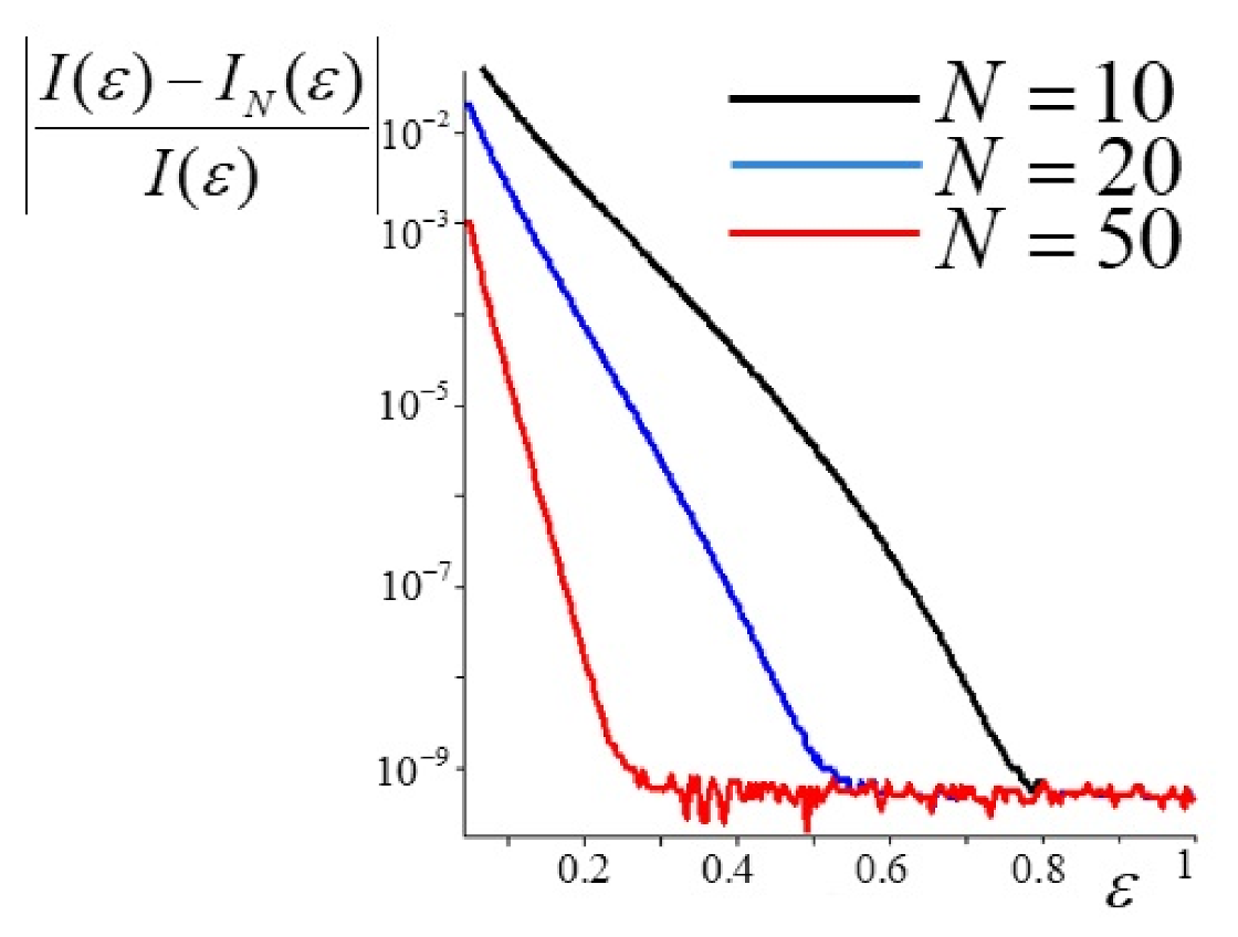
From the above expression, we see that $I\left(ϵ\right)$ is an increasing function of $ϵ$, from $I(ϵ=0)=0$ to $I(ϵ=1)=\frac{4{\pi }^4}{45}\sim 8.6586$. At order N, the approximation $I_N\left(ϵ\right)$ of $I\left(ϵ\right)$ is expressed by

$$I\left(ϵ\right)\sim I_N\left(ϵ\right)=\frac{4{\pi }^4}{45}-\frac{{\pi }^4}{15}(1-ϵ)-2\sum _{n=2}^N{c}_n{(1-ϵ)}^n,$$

(25)

For $ϵ$ in the range $(0.05,1)$, the relative errors $|\frac{I\left(ϵ\right)-I_N\left(ϵ\right)}{I\left(ϵ\right)}|$ for $N=10$, $N=20$, and $N=50$ are reported in Figure 2: the maximum relative error for $N=20$ is about 2.1%, whereas for $N=50$, this maximum corresponds to about 0.11%.

Once the value of $I\left(ϵ\right)$ has been fixed, numerically or by the approximation Equation (25), we can obtain from Equation (18) the entropy rate for unit surface $d\dot{s}$ by dividing it by the volume and by multiplying by the speed of light c [11,15], giving

$$d\dot{s}=\frac{16\sigma }{3}I\left(ϵ\right)T^3.$$

(26)

Hence, the entropy rate due to radiative processes is obtained by integration over the entire fin. With the same approximation as in Equation (2), one obtains

$${\left.{\dot{s}}_{\sigma }\right|}_{T_{in}\to T}=2L\frac{16\sigma }{3}I\left(ϵ\right){\int }_0^{\ell }(T^3-T_{in}^3)dx.$$

(27)

The total entropy rate (in W/°K) of the fin by convection and radiation is found by summing up the two contributions (8) and (27):

$${\left.\dot{s}\right|}_{T_{in}\to T}={\left.{\dot{s}}_h\right|}_{T_{in}\to T}+{\left.{\dot{s}}_{\sigma }\right|}_{T_{in}\to T}=2L{\int }_0^{\ell }\left(hln\left(\frac{T}{T_{in}}\right)+\frac{16\sigma }{3}I\left(ϵ\right)(T^3-T_{in}^3)\right)dx.$$

(28)

3. An Entropy-Based Indicator for the Efficiency of the Fin in Its Steady State

Efficiency is a widely adopted indicator for the capability of a fin to dissipate heat [1,2,16]. Before the introduction of physical indicators, there is usually a definition of some reference state of the system under consideration. This is the case also for efficiency. The reference state, implicitly given in the definition of efficiency, is given by the fin at the constant temperature equal to the temperature of the base $T_b$ ($\theta =1$). Accordingly, the efficiency $\eta$ of the fin is defined as the ratio of two terms: in the numerator, one has the actual heat transfer; in the denominator, one has the ideal heat transfer for a fin with an infinite thermal conductivity in the reference state. This efficiency for the steady state solution of Equation (5) can be also written as [4]

$$\eta =\frac{B{i}_1({\theta }_0-\theta \left(1\right))+B{i}_0(1-\theta \left(0\right))+N_1(\varphi {\theta }_0^4-\theta {\left(1\right)}^4)+N_0(\varphi -\theta {\left(0\right)}^4)}{\alpha (1-{\theta }_0)+\beta (1-\varphi {\theta }_0^4)}.$$

(29)

In the following, we define an efficiency on the base of the amount of entropy produced by the fin in the process of dissipation of heat by convection and radiation. Furthermore, to make a comparison with the classical efficiency (29), the definition of the entropy rate $\dot{s}$ must include the same reference state. More comments will be given in the following about the reference state of our definition. Now, let us calculate the difference between the entropy produced by the fin by evolving the system from $T_{in}$ to $T_b$ and the entropy produced by evolving the system from $T_{in}$ to a suitable T:

$$\dot{s}:={\left.\dot{s}\right|}_{T\to T_b}={\left.\dot{s}\right|}_{T_{in}\to T_b}-{\left.\dot{s}\right|}_{T_{in}\to T},$$

(30)

i.e., by applying (28):

$$\dot{s}=2L{\int }_0^{\ell }\left(\frac{16\sigma }{3}I\left(ϵ\right)(T_b^3-T^3)-hln\left(\frac{T}{T_b}\right)\right)dx.$$

(31)

We introduce, for greater clarity, a reference convective entropy rate ${\dot{s}}_{0,h}$ and a reference radiative entropy rate ${\dot{s}}_{0,\sigma }$:

$${\dot{s}}_{0,h}=2L\ell h,{\dot{s}}_{0,\sigma }=2L\ell \frac{16\sigma }{3}I\left(ϵ\right)T_b^3.$$

(32)

These two entropies correspond respectively to the entropies produced by the fin by evolving the system from $T_{in}$ to $exp\left(1\right)T_{in}$ and from $T=0$ to $T_b$. The expression (31) then becomes

$$\dot{s}={\int }_0^1\left({\dot{s}}_{0,\sigma }(1-{\theta }^3)-{\dot{s}}_{0,h}ln\left(\theta \right)\right)dz.$$

(33)

As said, the classical efficiency is equal to the ratio between the actual heat transfer to the ideal heat transfer for a fin at temperature $T_b$. Our definition of the entropic efficiency is the ratio between the entropy produced by the fin during the evolution of the system from the initial temperature $T_0$ to the steady state T with respect to the entropy produced by the fin by evolving the system from the same initial distribution $T_0$ to the reference temperature $T_b$. We notice that the steady state T is independent of the initial distribution temperature $T_{in}$: as the initial state, we then take $T_0$. It follows that the indicator giving the entropy-based effectiveness of the fin to dissipate heat by convection and radiation can be defined as fp;;pws:

$${\eta }_s\doteq \frac{{\int }_0^1\left({\dot{s}}_{0,\sigma }({\theta }^3-{\theta }_0^3)-{\dot{s}}_{0,h}ln\left(\frac{{\theta }_0}{\theta }\right)\right)dz}{\left({\dot{s}}_{0,\sigma }(1-{\theta }_0^3)-{\dot{s}}_{0,h}ln\left({\theta }_0\right)\right)}=1-\frac{{\int }_0^1\left({\dot{s}}_{0,\sigma }(1-{\theta }^3)-{\dot{s}}_{0,h}ln\left(\theta \right)\right)dz}{\left({\dot{s}}_{0,\sigma }(1-{\theta }_0^3)-{\dot{s}}_{0,h}ln\left({\theta }_0\right)\right)}.$$

(34)

As it should be, if $\theta \left(z\right)={\theta }_0$, then ${\eta }_s=0$, whereas ${\eta }_s=1$ when $\theta \left(z\right)={\theta }_b=1$. By looking at the definitions before Equation (5), we see that the ratio between the reference entropies ${\dot{s}}_{0,\sigma }$ and ${\dot{s}}_{0,h}$ is proportional to the ratio of $\alpha$ and $\beta$, i.e., the dimensionless convective and radiative coefficients:

$$\frac{{\dot{s}}_{0,\sigma }}{{\dot{s}}_{0,h}}=\frac{16}{3}\frac{I\left(ϵ\right)}{ϵ}\frac{\beta }{\alpha }$$

(35)

Therefore, Equation (34) can also be written in the following form:

$${\eta }_s=\frac{{\int }_0^1\left(\frac{16}{3}\frac{I\left(ϵ\right)}{ϵ}\beta ({\theta }^3-{\theta }_0^3)-\alpha ln\left(\frac{{\theta }_0}{\theta }\right)\right)dz}{\left(\frac{16}{3}\frac{I\left(ϵ\right)}{ϵ}\beta (1-{\theta }_0^3)-\alpha ln\left({\theta }_0\right)\right)}=1-\frac{{\int }_0^1\left(\frac{16}{3}\frac{I\left(ϵ\right)}{ϵ}\beta (1-{\theta }^3)-\alpha ln\left(\theta \right)\right)dz}{\left(\frac{16}{3}\frac{I\left(ϵ\right)}{ϵ}\beta (1-{\theta }_0^3)-\alpha ln\left({\theta }_0\right)\right)}$$

(36)

As a final note, let us calculate the difference between the entropy rate produced by the fin during the evolution of the system from the temperature $T_0$ to the steady state T and the entropy rate produced by the fin by evolving the system from the same initial distribution $T_0$ to the reference temperature $T_b$. This is the difference between the numerator and the denominator of Equation (36). We get

$$\begin{array}{cc}\hfill & {\left.\dot{s}\right|}_{T_0\to T}-{\left.\dot{s}\right|}_{T_0\to T_b}=\left({\dot{s}}_{0,\sigma }({\theta }^3-{\theta }_0^3)-{\dot{s}}_{0,h}ln\left(\frac{{\theta }_0}{\theta }\right)\right)dz-\left({\dot{s}}_{0,\sigma }(1-{\theta }_0^3)-{\dot{s}}_{0,h}ln\left({\theta }_0\right)\right)dz\hfill \\ \hfill & ={\int }_0^1\left({\dot{s}}_{0,\sigma }({\theta }^3-1)+{\dot{s}}_{0,h}ln\left(\theta \right)\right)dz\hfill \end{array}$$

(37)

Notice that, since $T_b>T_0$ (i.e., ${\theta }_0<1$), the temperature $\theta \left(z\right)$ is expected to be a decreasing function of z and hence $\theta <1$ for every point of the fin. The difference in (37) is then always negative, implying ${\eta }_s<1$. Physically, this means that the reference state $T_b$ is the state expected to possess the maximum entropy rate.

In the next section, we start to analyze the purely convective case and to investigate the reliability of the definition (36). Additionally, we make a comparison with the classical definition of the efficiency (29).

4. The Pure Convective Case

For a fin dissipating heat solely through the convective mechanism, Equation (34) for the efficiency becomes

$${\eta }_s=1-\frac{1}{ln\left({\theta }_0\right)}{\int }_0^{1}ln\left(\theta \right)dz.$$

(38)

The simplest case is that of a rectangular longitudinal profile. In this case, the dimensionless profile is given by $f\left(z\right)=1$. The solution of Equation (5) with the boundary conditions (6) gives the steady state temperature $\theta \left(z\right)$. This function, given in [4], is

$$\theta \left(z\right)={\theta }_0+(1-{\theta }_0)B{i}_0\frac{mcosh\left(m(1-z)\right)+B{i}_{1}sinh\left(m(1-z)\right)}{m(B{i}_0+B{i}_1)cosh\left(m\right)+(m^2+B{i}_{0}B{i}_1)sinh\left(m\right)}.$$

(39)

The previous formula allows us to obtain the temperature distribution along a fin with a base at $T=T_b$ and an insulated tip. It is sufficient to take $B{i}_1=0$ and to make the limit $B{i}_0\to \infty$. In this case, Equation (39) reduces to

$$\theta \left(z\right)={\theta }_0+(1-{\theta }_0)\frac{cosh\left(m\right(1-z\left)\right)}{cosh\left(m\right)}.$$

(40)

From Equation (38), the corresponding value of the entropic efficiency is

$${\eta }_s=-\frac{1}{ln\left({\theta }_0\right)}{\int }_0^{1}ln\left(1+acosh\left(my\right)\right)dy,$$

(41)

where $a=\frac{1-{\theta }_0}{cosh\left(m\right){\theta }_0}$. As explained in the Introduction, we expect that the efficiency is also a function of the temperature of the fluid, and it is thought that the Gardner result (valid for a rectangular fin with an insulated tip, exactly as in this case) gives accurate results for small values of the temperature gradient between the base and the fluid. Then, to test the consistency of our definition of the efficiency (34), we calculate the limit ${\theta }_0\to 1$ (small gradients) and determine if the limit is in agreement with the Gardner’s result. In the limit ${\theta }_0\to 1$, we get for the integrand on the right-hand side of (41)

$$-\frac{ln\left(1+acosh\left(my\right)\right)}{ln\left({\theta }_0\right)}=\frac{cosh\left(my\right)}{cosh\left(m\right)}+\frac{1}{2}\left(\frac{cosh\left(my\right)}{cosh\left(m\right)}-\frac{cosh{\left(my\right)}^2}{cosh{\left(m\right)}^2}\right)(1-{\theta }_0)+O\left({(1-{\theta }_0)}^2\right)$$

(42)

The corresponding value of the efficiency is then given by

$${\eta }_s=\frac{tanh\left(m\right)}{m}+\frac{1}{8}\frac{sinh\left(2m\right)-2m}{2m(1+cosh(2m\left)\right)}(1-{\theta }_0)+O\left({(1-{\theta }_0)}^2\right)$$

(43)

Gardner’s classical results about the efficiency corresponding to a temperature profile given by (40) is given by [4,16]

$$\eta =\frac{tanh\left(m\right)}{m}$$

(44)

Therefore formula (43) can be rewritten as

$${\eta }_s=\eta +\frac{1}{8}\frac{sinh\left(2m\right)-2m}{2m(1+cosh(2m\left)\right)}(1-{\theta }_0)+O\left({(1-{\theta }_0)}^2\right)$$

(45)

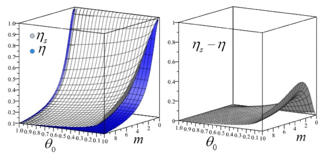
As it can be seen from this example, (38) can be considered an extension, based on the quantity of heat dissipated by the fin, of the classical definition of efficiency. In Figure 3, we plot efficiency (41) and efficiency (44) as a function of ${\theta }_0$ and m (left) and the difference between formula (41) and the classical formula (44). The observation that the entropic efficiency ${\eta }_s$ (38) reduces to the classical efficiency $\eta$ (29) when ${\theta }_0\to 1$ is not peculiar to this particular example and fin profile but, as we will see in the next subsection, holds for any arbitrary profile. This gives further support to the effectiveness of our definition (36).

In the case of a purely convective fin with an arbitrary profile, the steady state is described in dimensionless variables by the following equation:

$$\frac{d}{dz}\left(f\left(z\right)\frac{d\theta }{dz}\right)=\alpha (\theta -{\theta }_0)$$

(46)

For the sake of simplicity let us consider the case of a fin with an insulated tip and the base at the constant temperature $T_b$ (i.e., $\theta =1$). The boundary conditions (6) are given in this case by

$$\begin{array}{cc}\hfill & {\left.(\theta -1)\right|}_{z=0}=0,\hfill \\ \hfill & {\left.\frac{d\theta }{dz}\right|}_{z=1}=0.\hfill \end{array}$$

(47)

In [4], it has been shown that the following change in variable is particularly useful:

$$\theta \left(z\right)=F\left(y\left(z\right)\right),\mathrm{with}f\left(z\right)\frac{dy}{dz}=1.$$

(48)

Indeed, thanks to the previous definition of $y\left(z\right)$, Equation (46) becomes

$$\frac{d^{2}F}{d{y}^2}=\alpha f\left(z\right)(F\left(y\right)-{\theta }_0).$$

(49)

By taking into account the boundary conditions, it is possible to make explicit the dependence on ${\theta }_0$ of the function $F\left(y\right)$. The solution of Equation (49) can be written as

$$F\left(y\right)={\theta }_0+(1-{\theta }_0)g\left(y\right)$$

(50)

where $g\left(y\right)$ solves $\frac{d^{2}g}{d{y}^2}=\alpha f\left(z\right)g\left(y\right)$ with boundary conditions given by ${\left.g\left(y\right)\right|}_{z=0}=1$ and ${\left.\frac{dg}{dy}\right|}_{z=1}=0$. This implies that $g\left(y\right)$ is independent of ${\theta }_0$. The entropic efficiency (38) of the fin is written as

$${\eta }_s=1-\frac{1}{ln\left({\theta }_0\right)}{\int }_0^{1}ln\left(\theta \right)dz=-\frac{1}{ln\left({\theta }_0\right)}{\int }_0^{1}ln\left(1+\frac{1-{\theta }_0}{{\theta }_0}g\left(y\right)\right)dz$$

(51)

In the limit ${\theta }_0\to 1$, we get

$${\eta }_s={\int }_0^{1}g\left(y\right)dz+\frac{(1-{\theta }_0)}{2}{\int }_0^1\left(g\left(y\right)-g{\left(y\right)}^2\right)dz+O\left({(1-{\theta }_0)}^2\right).$$

(52)

Let us look at the classical definition of the entropy. From [4] (see Equation (15)), we have in terms of the function $F\left(y\right)$ defined in Equation (48)

$$\eta \doteq \frac{1}{\alpha (1-{\theta }_0)}\left({\left.\frac{dF}{dy}\right|}_{z=1}-{\left.\frac{dF}{dy}\right|}_{z=0}\right)=\frac{1}{\alpha (1-{\theta }_0)}{\int }_0^1\frac{d}{dz}\left(\frac{dF}{dy}\right)dz=\frac{1}{\alpha (1-{\theta }_0)}{\int }_0^1\frac{d^{2}F}{d{y}^2}\frac{dy}{dz}dz.$$

(53)

However, by multiplying Equation (49) for $\frac{dy}{dz}$ and by using the constraint $f\left(z\right)\frac{dy}{dz}=1$, it follows that $\frac{d^{2}F}{d{y}^2}\frac{dy}{dz}=\alpha (F\left(y\right)-{\theta }_0)$, giving

$$\eta =\frac{1}{1-{\theta }_0}{\int }_0^1(F\left(y\right)-{\theta }_0)dz$$

(54)

or, from Equation (50),

$$\eta ={\int }_0^{1}g\left(y\right)dz.$$

(55)

The previous result confirms that the classical efficiency of a convective fin is independent from the temperature of the fluid and furthermore shows that, for small values, the difference in temperature between the base of the fin and the fluid the two definitions of efficiency, ${\eta }_s$ (38) and $\eta$ (29), give the same value. This result is general does not depend on the fin profile or the temperature distribution across the fin, since the function g in (50) is arbitrary. In the next section, the more general convective-radiative case will be considered.

5. The Convecting-Radiating Fin and Its Efficiency

If the fin dissipates heat both by convection and radiation, the differential equation describing the steady state becomes nonlinear and it is very challenging, in general, to find out solutions general solutions. However, a family of explicit solutions have been described in [4]: the solutions have been written in terms of an auxiliary function $y\left(z\right)$ introduced by a change of variables. The boundary conditions are similar to the ones given by Equation (6). For completeness, we report the corresponding principal formulae and we restrict the discussion to gray fins. From a mathematical point of view, this means setting $\varphi =1$ in Equations (5) and (6).

Let us make the following change in variables:

$$\theta \left(z\right)={\theta }_0+wy{\left(z\right)}^2,w\in \mathbb{R}.$$

(56)

and assume that it holds the constraint $f\left(z\right)\frac{dy}{dz}=1$. Then, by integrating the steady version of Equation (5), one gets the following implicit formula for $y\left(z\right)$ [4]:

$$\begin{array}{cc}& -\frac{A}{y}+E_{1}arctan\left(\frac{y}{b_1}\right)+E_2\left(arctan\left(\frac{y+a_2}{b_2}\right)+arctan\left(\frac{y-a_2}{b_2}\right)\right)+F_{2}ln\left(\frac{{(y+a_2)}^2+b_2^2}{{(y-a_2)}^2+b_2^2}\right)\hfill \\ \hfill & =\frac{\beta w^3}{2}(z+C),\hfill \end{array}$$

(57)

where the values of A, $E_1$, $E_2$, and $F_2$ are given by

$$\begin{array}{cc}\hfill & E_1=-\frac{1}{b_1^3\left(a_2^2+{(b_1-b_2)}^2\right)\left(a_2^2+{(b_1+b_2)}^2\right)},\hfill \\ \hfill & E_2=\frac{1}{4}\frac{\left((a_2^2-3b_2^2)(a_2^2+b_1^2-b_2^2)-2b_2^2(3a_2^2-b_2^2)\right)}{\left(a_2^2+{(b_1-b_2)}^2\right)\left(a_2^2+{(b_1+b_2)}^2\right){\left(a_2^2+b_2^2\right)}^3{b}_2},\hfill \\ \hfill & A=\frac{1}{b_1^2{(a_2^2+b_2^2)}^2},F_2=\frac{1}{8}\frac{\left((b_2^2-3a_2^2)(a_2^2+b_1^2-b_2^2)+2a_2^2(3b_2^2-a_2^2)\right)}{\left(a_2^2+{(b_1-b_2)}^2\right)\left(a_2^2+{(b_1+b_2)}^2\right){\left(a_2^2+b_2^2\right)}^3{a}_2}.\hfill \end{array}$$

In these expressions, the coefficients $b_1$, $a_2$, and $b_2$ can be given in terms of the ratio $\alpha /\beta$, the dimensionless fluid temperature ${\theta }_0$, and the parameter w appearing in (56). One has

$$b_1=\sqrt{\frac{2{\theta }_0+b}{w}},a_2^2=\frac{b-2{\theta }_0+2\sqrt{2{\theta }_0^2+b^2}}{4w},b_2^2=\frac{2{\theta }_0-b+2\sqrt{2{\theta }_0^2+b^2}}{4w}.$$

(58)

In the previous expressions, the value of b is given by the unique real solution of a cubic equation:

$$\frac{\alpha }{\beta }=b(b^2+2b{\theta }_0+2{\theta }_0^2).$$

(59)

It remains to fix the values of w, appearing in (56), and the constant C, appearing in (57). One must set the boundary condition at $z=0$. The first of the two boundary conditions (6) can be written as a polynomial equation for ${y\left(0\right)=y|}_{z=0}$ (see [4]):

$$B{i}_0(wy{\left(0\right)}^2-(1-{\theta }_0))+N_0\left({(wy{\left(0\right)}^2+{\theta }_0)}^4-1\right)-2wy\left(0\right)=0.$$

(60)

It is also possible to show that, for fixed values of $B{i}_0$, $N_0$, ${\theta }_0$ and w, the previous equation always has one real negative solution (see [4]). Let us call this solution $y_{-}$. The initial condition for y is then fixed by $y\left(0\right)=y_{-}$.

The value of w must be fixed, for consistency, by considering the assumed constraints $f\left(z\right)\frac{dy}{dz}=1$ and $f\left(0\right)=1$. One obtains

$$f\left(0\right)=1=\frac{2}{\beta y_{-}^2\left(w{y}_{-}^2+2{\theta }_0+b\right)\left({\left(w{y}_{-}^2+{\theta }_0-\frac{b}{2}\right)}^2+{\theta }_0({\theta }_0+b)+\frac{3}{4}{b}^2\right)}.$$

(61)

The value of C can be found by evaluating Equation (57) at $y=y_{-}$ and $z=0$. At this point, the function $y\left(z\right)$ is completely determined by Equation (57) for any arbitrary choice of the parameters $\beta$ and b. The corresponding values of the dimensionless temperature $\theta \left(z\right)$, corresponding to the steady state, are finally found from (56).

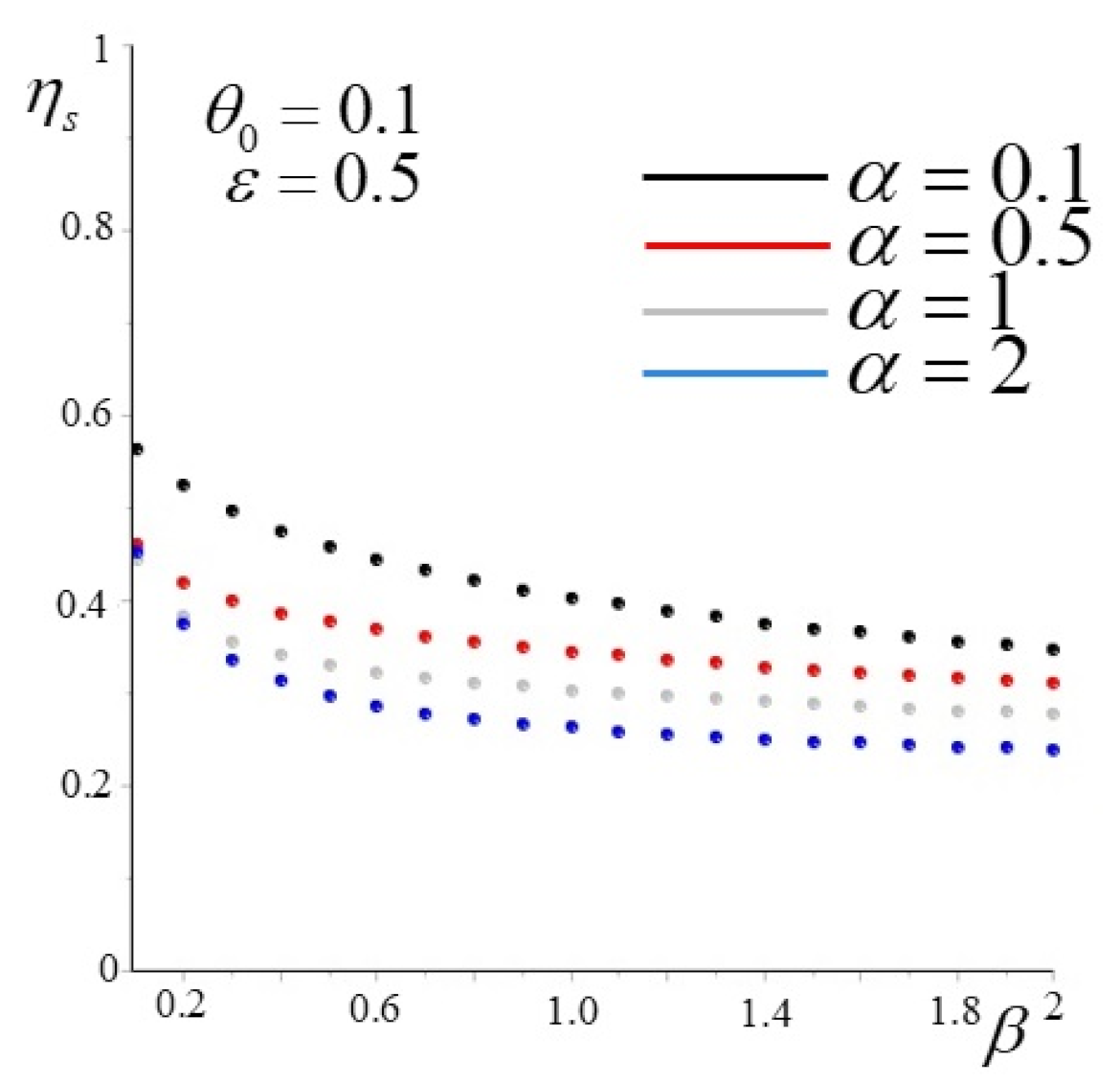
Now, we apply the methodology reported above to describe the dependence of the entropic efficiency (36) on the dimensionless convection and radiation coefficients $\alpha$ and $\beta$ and on the emissivity $ϵ$.

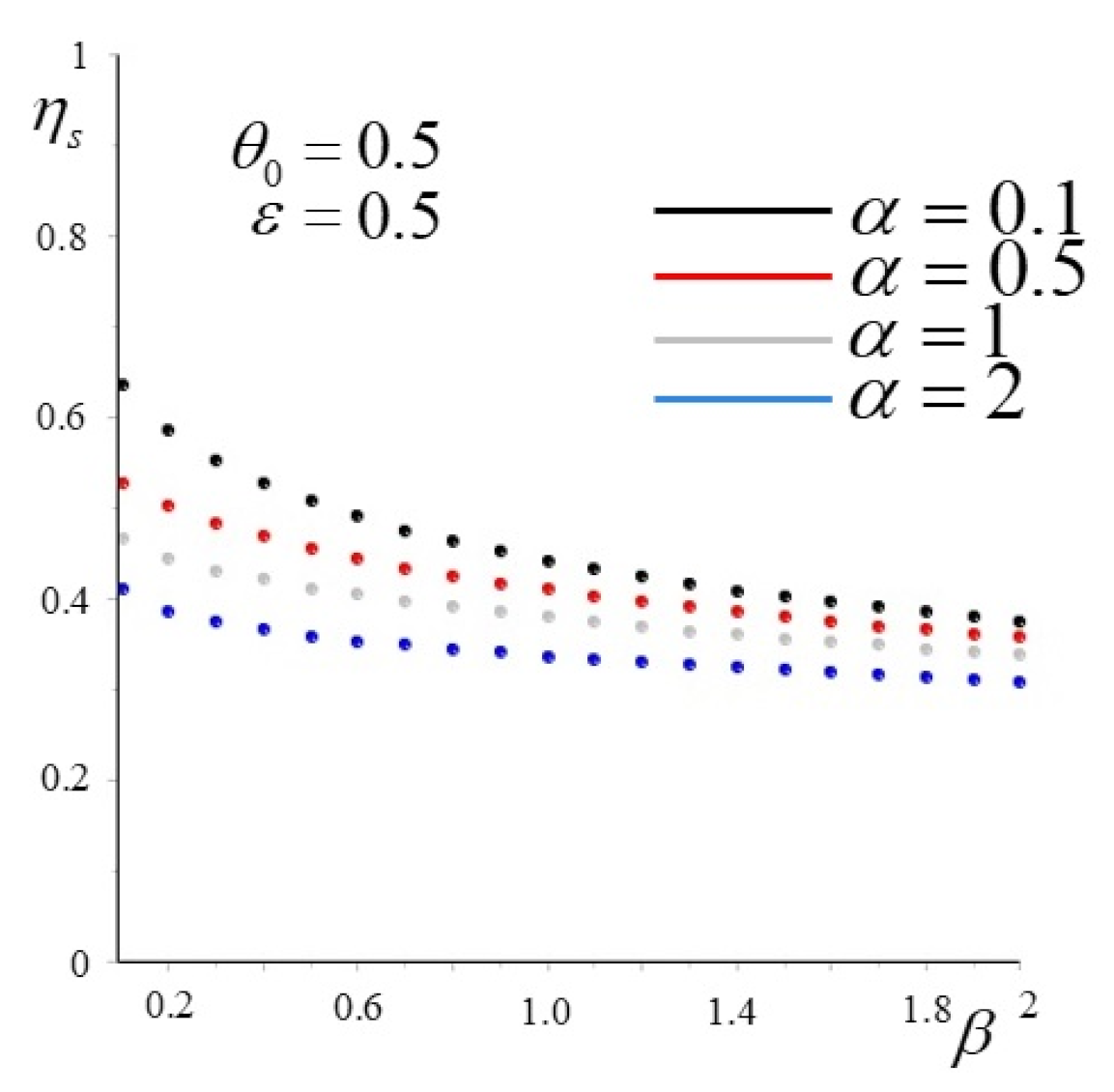
For simplicity, let us consider the case of a fin with a base at $T=T_b$, i.e., $\theta \left(0\right)=1$. This corresponds to $B{i}_0\to \infty$ and/or $N_0\to \infty$. It can be shown that, in this case, w can also be written as

$$w=\frac{1}{2}\left(\alpha (1-{\theta }_0)+\beta (1-{\theta }_0^4)\right).$$

(62)

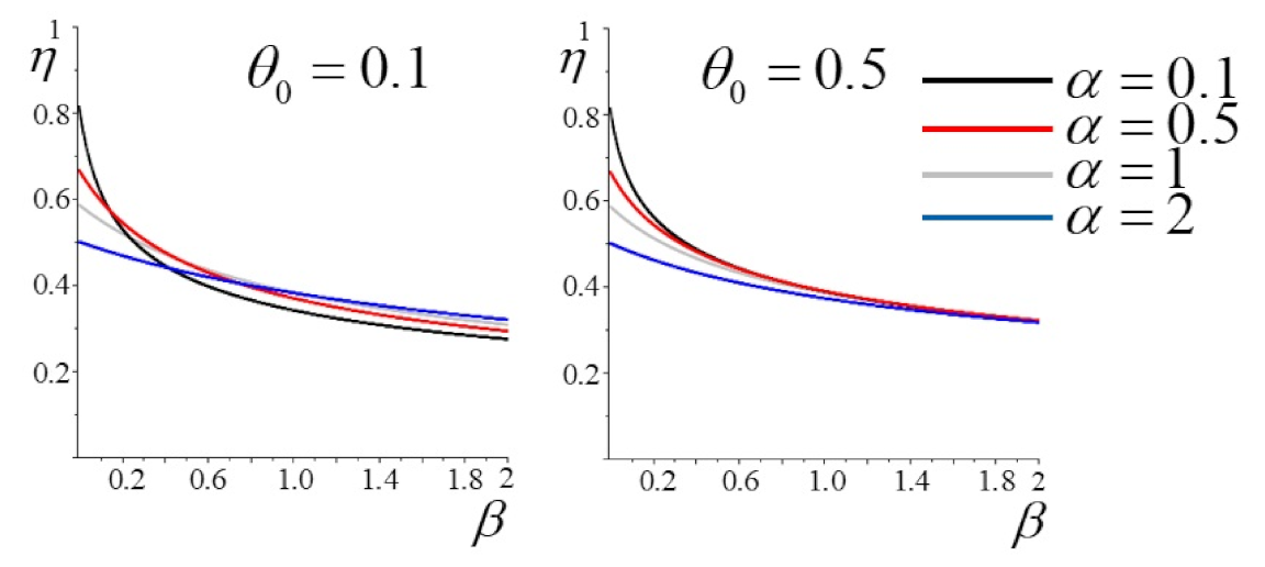
Let us further assume that, to fix the ideas, the emissivity is equal to $ϵ=0.5$. The corresponding value of $I\left(ϵ\right)$ (19) is $I\left(ϵ\right)\sim 5.097$. We choose two different values of ${\theta }_0$: ${\theta }_0=0.1$ and ${\theta }_0=0.5$. For each of these choices, it is possible to consider different values of $\alpha$. We take four different values of this parameter, namely $\alpha =\{0.1,0.5,1,2\}$. Additionally, it remains to choose $\beta$. We take twenty different values, from $\beta =0.1$ to $\beta =2$, equally spaced. For each one of these choices, we calculate the distribution of temperatures along the fin according to Equations (56) and (57). Finally, we calculate the entropic efficiency of each state by means of Equation (36). The results are given in Figure 4 and Figure 5: as it is possible to see, in all cases, the efficiency decreases by increasing the values of $\beta$ and decreases by increasing the values of $\alpha$. If one looks at a simialr variation of the parameters for the classical efficiency, it follows that the behavior of ${\eta }_s$ is in agreement with that of the classical efficiency (29). For comparison, we report in Figure 6 also the corresponding values of the classical efficiencies, calculated with Equation (29) (see [4]).

6. An Example with Convecting-Radiating Aluminum Fins.

In the previous example, we made use of dimensionless quantities. As it has been pointed out in [4], thanks to the dimensionless form of the equations, the high number of physical constants have been replaced by only a few parameters, i.e., $\alpha$, $\beta$, and ${\theta }_0$. In this way, the relative importance of the convective and radiative terms can be easily assessed [4]. On the other hand, our analytical treatment assumes that the thermal coefficients (i.e., the thermal conductivity, the convective heat transfer coefficient, and the emissivity) are constants. For real materials, this is true only for finite ranges of variation in temperature, and this must be taken into account in the applications of the above results.

In [4], the relative importance of the convective and radiative effects has been shown by making a practical example without dimensionless quantities. The fin was assumed to be made of aluminum, with $ϵ=0.9$ for anodized aluminum. The base was at 800 K, and the fluid was at 400 K. The thermal conductivity for aluminum is almost constant between 400 K and 800 K, since it varies from 220 Wm${}^{-1}$ K${}^{-1}$ to 240 Wm${}^{-1}$ K${}^{-1}$ [17]. Two cases were analyzed, with the only difference being the values of the heat transfer coefficients, given by 50 ${\mathrm{Wm}}^{-2}{\mathrm{K}}^{-1}$ and 250 ${\mathrm{Wm}}^{-2}{\mathrm{K}}^{-1}$. These two values correspond respectively to the values $(\alpha ,\beta )=(0.4348,0.2272)$ and $(\alpha ,\beta )=(2.1739,0.2272)$. We do not report the distribution of temperature across the fin for the two cases. The interested readers can refer to [4]. Instead, we analyze the distribution of the entropic efficiency as a function of the heat transfer coefficient and compare these values with those of the classical efficiency.

We divide the $\mathtt{h}=[50,250]{\mathrm{Wm}}^{-2}{\mathrm{K}}^{-1}$ (or the interval $\alpha =[0.4348,2.1739]$) in twenty sub-intervals and calculate the entropic efficiency for each of these intervals. We calculate the distribution of the temperature according to Equations (56) and (57) and then the values of the entropic efficiency through Equation (36). We analyze the case of a fin with a base at $T=T_b$, i.e., $\theta \left(0\right)=1$. The other values of the constants appearing in the steady version of Equation (2) determining the values of $\alpha$ and $\beta$ are the following: the ratio ${\ell }^2/f_b$ is fixed to be equal to 1 m (if both ℓ and $f_b$ are in cm, $\ell =10\sqrt{f_b}$), whereas we fix the thermal conductivity of the aluminum to be equal to $\kappa =230\mathrm{W}{\mathrm{m}}^{-1}{\mathrm{K}}^{-1}$ between 400 K and 800 K. For $ϵ=0.9$, the ratio $I\left(ϵ\right)/ϵ$, where $I\left(ϵ\right)$ is given by Equation (19), is equal to 8.8875.

After, we plot the corresponding values of the classical efficiency. Formula (29), in the case of a fin with a base at a temperature equal to $T_b$ and for a gray fin (i.e., $\varphi =1$ in Equations (5) and(6), it is possible to show that the classical efficiency is simply given by [4]:

$$\eta =y\left(1\right)-y\left(0\right),$$

(63)

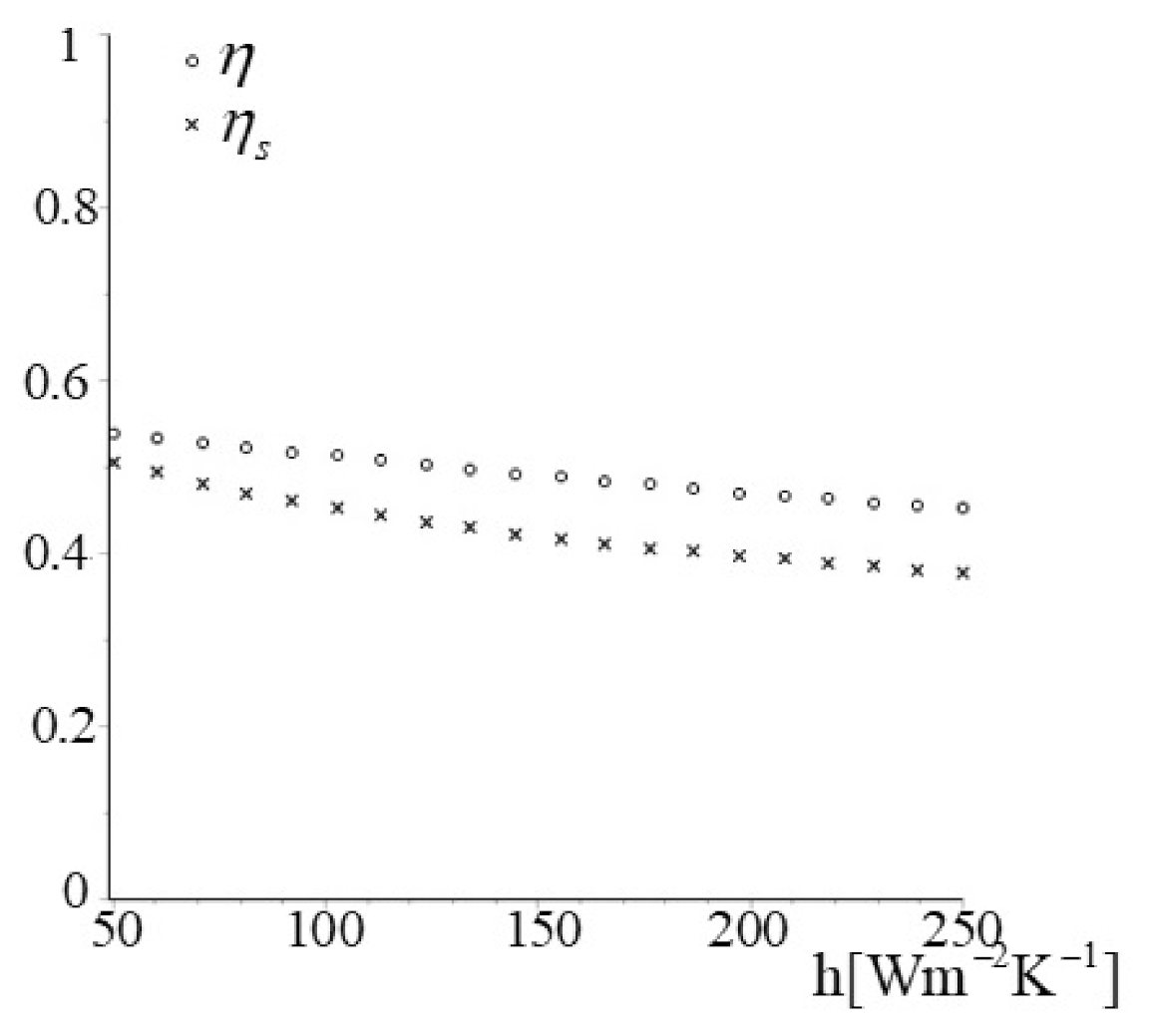
where $y\left(z\right)$ is the auxiliary function appearing in Equation (56) for the dimensionless temperature. The results are reported in Figure 7.

As can be seen from the figure, both the efficiencies decrease as functions of $\mathtt{h}$, but the entropic efficiency is always lower, in this particular case, with respect to the classical efficiency. This is in contrast to what happens for the purely convective case. Indeed, if we take Equations (51) and (55), the difference $\eta -{\eta }_s$ can be written as

$$\eta -{\eta }_s={\int }_0^1\left(g\left(y\right)+\frac{1}{ln\left({\theta }_0\right)}ln\left(1+\frac{1-{\theta }_0}{{\theta }_0}g\left(y\right)\right)\right)dz$$

(64)

For $T_b>T_0$, the temperature is expected to be a decreasing function of z (actually, it has been noticed in [4] that, for a suitable choice of parameters describing the boundary conditions, the temperature may possess a minimum in the interval $z\in (0,1)$. For simplicity we avoid such values of the parameters). In this case, the function $g\left(y\right)$ is always bounded in the interval $[0,1]$, similar to ${\theta }_0$. Then, it can be shown that the integrand in Equation (64) is always negative, giving a value of the classical efficiency smaller than the value of the entropic efficiency. A deeper analysis of the properties of formula (34) by varying the parameters $\alpha ,\beta ,ϵ$, and ${\theta }_0$ and the comparison with the corresponding values of the classical efficiency is necessary to provide a further characterization of the function ${\eta }_s$ and will be one of the subjects of a forthcoming paper.

7. Conclusions

We introduced a novel indicator of the performances of longitudinal fins of arbitrary profile. The indicator takes into account the amount of entropy rate produced by the fin by approaching its steady state. The contributions to the entropy considered are those coming from convection and radiation. We have shown that the values of efficiencies given by the definition and those obtained by the classical formula are compatible in a suitable approximation. In our opinion, the new definition is however more flexible: indeed, the role of the fluid temperature is explicit in opposition to the classical formulation. This has been shown for the convective case with an arbitrary profile, and for example, it is particularly evident from Equations (45) and (55). If, on the one hand, this new indicator rests on the concept of entropy and, as such, we expect to reflect the content of the second principle of thermodynamics (see also [18] for a discussion on this aspect), on the other hand, we are aware of the fact that a proper evaluation of its efficacy and adherence to the physical reality needs a deeper assessment. The definition of the indicator (36) relies on the introduction of a reference state. The reference state of the classical efficiency (29) is given by the temperature $T_b$ of the base of the fin. We take the reference state of the new indicator to be the same. This choice is fundamental for two main reasons:

(i)

The idea underlying Equation (36) is the following: to measure the dissipation, through entropy rates, of the steady state of the fin with respect to that of an ideal fin with the highest dissipation possible. If the real fin is close to this ideal fin, the corresponding efficiency will be higher. The reference state $T_b$, as it has been shown at the end of Section (Section 3), is also the state expected to possess the maximum entropy rate.

(ii)

The classical definition of the efficiency $\eta$ is given by the ratio of the actual heat transfer over the ideal heat transfer for a fin at temperature equal $T_b$. Since we take the reference state for the entropic efficiency to be the same, we have the possibility to make a direct comparison between the two definitions.

Furthermore, we emphasize that, in our approach, there is no use of any variational principle. We compare the entropy rates of two possible states: the reference state, at temperature $T_b$, and the steady state solution of the classical Fourier equation. To analyze both the convective and the full convective-radiative cases, we used some of the results that appeared in [4]. In that work, explicit formulae for the steady solutions of the temperature along the fin have been obtained. A new approximated formula for the integral giving the entropy of the radiation as a function of the emissivity has been given. Additionally, we have shown that, for the purely convective case, the entropic efficiency reduces to the classical definition for small temperature gradients and that the classical definition gives smaller values of the efficiency. This last observation is not true for the convecting-radiating fin, as can be seen from the discussion at the end of Section 6; see also Figure 7. We are aware of the fact that the geometric properties of the fin are only a particular aspect of the fin optimization, since the material, its manufacturability and cost, and its weight (for aerospace applications) are other aspects that may become relevant (or not) in specific applications. Clearly, it is not possible to examine all these aspects in this paper. The interested reader can look for examples in [1,2] and the references therein. On the other hand, we expect that this work is a starting point for a more in-depth analysis of the efficiency of fins. Different mechanisms of heat dissipation and profiles can be considered. The possibility to extend the results to 2D or 3D models will be analyzed in future works: we underline that the methodology developed here is fairly general and we believe that it is worth taking into further consideration to be applied to more complex cases. Another very interesting and physically more complete direction of research will be to enlarge the model to include a stress-deformation analysis. The starting point may be decoupling of the thermal effect from the Newton–Hooke equations for elastic response: we expect that a corresponding entropy term is added to Equation (28) and that the definition of the efficiency should change accordingly. The possibility to include these effects to the example given in Section 6 will be also investigated in a next work.

References

- Kraus, A.D.; Aziz, A.; Welty, J.R. Extended Surface Heat Transfer; Wiley: New York, NY, USA, 2002. [Google Scholar]
- Howell, J.R.; Mengüç, M.P.; Siegel, R. Thermal Radiation Heat Transfer, 6th ed.; CRC Press: Boca Raton, FL, USA, 2016. [Google Scholar]
- Krane, R.J. Discussion on Perturbation Solution for Convecting Fin with Variable Thermal Conductivity. J. Heat Transf. 1976, 98, 585. [Google Scholar]
- Bochicchio, I.; Naso, M.G.; Vuk, E.; Zullo, F. Convecting-radiating fins: Explicit solutions, efficiency and optimization. Appl. Math. Model. 2021, 89, 171–187. [Google Scholar] [CrossRef]
- Giorgi, C.; Zullo, F. Entropy Production and Efficiency in Longitudinal Convecting–Radiating Fins. Proceedings 2020, 58, 13. [Google Scholar] [CrossRef]
- Nicolini, G.; Sciubba, E. Minimization of the Local Rates of Entropy Production in the Design of Air Cooled Gas Turbine Blades. J. Eng. Gas Turbines Power 1999, 121, 466–475. [Google Scholar]
- Sciubba, E.; Zullo, F. A Novel Derivation of the Time Evolution of the Entropy for Macroscopic Systems in Thermal Non-Equilibrium. Entropy 2017, 19, 594. [Google Scholar] [CrossRef] [Green Version]
- Agudelo, A.; Cortes, C. Thermal radiation and the second law. Energy 2010, 35, 679–691. [Google Scholar] [CrossRef]
- Del Rio, F.; De la Selva, S.M.T. Reversible and irreversible heat transfer by radiation. Eur. J. Phys. 2015, 36. [Google Scholar] [CrossRef]
- Di Castro, C.; Raimondi, R. Statistical Mechanics and Applications in Condensed Matter; Cambridge University Press: Cambridge, UK, 2015; ISBN 978-1-107-03940-7. [Google Scholar]
- Kabelac, S.; Conrad, R. Entropy Generation During the Interaction of Thermal Radiation with a Surface. Entropy 2012, 14, 717–735. [Google Scholar] [CrossRef] [Green Version]
- Landsberg, P.T.; Tonge, G. Thermodynamics of the conversion of diluted radiation. J. Phys. A Math. Gen. 1979, 12, 551. [Google Scholar] [CrossRef]
- Schwabl, F. Statistical Mechanics; Springer: Berlin/Heidelberg, Germany, 2006; ISBN 13 978-3-540-32343-3. [Google Scholar]
- Wright, S.E.; Scott, D.S.; Haddow, J.B.; Rosen, M.A. On the entropy of radiative heat transfer in engineering thermodynamics. Int. J. Eng. Sci. 2001, 39, 1691–1706. [Google Scholar] [CrossRef]
- Fuchs, H.U. The Dynamics of Heat: A Unified Approach to Thermodynamics and Heat Transfer; Springer: Berlin/Heidelberg, Germany, 2010; ISBN 978-1-4419-7603-1. [Google Scholar]
- Gardner, K.A. Efficiency of Extended Surface. Trans. ASME 1945, 67, 621. [Google Scholar]
- Powell, R.W.; Ho, C.Y.; Liley, P.E. Thermal Conductivity of Selected Materials; Standards-8; US Government Printing Office: Washington, DC, USA, 1966.
- Laskowski, R.; Jaworski, M. Maximum entropy generation rate in a heat exchanger at constant inlet parameters. J. Mech. Energy Eng. 2017, 1, 79–86. [Google Scholar]
Figure 1.
The longitudinal fin: a given profile is shown, described by a suitable together with the coordinate system, the cross-sectional area, and the geometrical properties.
Figure 2.
Plots of the relative error for , , and . The scale is logarithmic. The peaks at the level of 10 are due to the numerical round-off error, since the calculation has been performed with 10 significant digits.
Figure 3.
The plot of efficiency (41) and (44) as a function of and m (left) and a plot of the difference between this efficiency and the classical formula (44) (right).
Figure 4.
The plot of efficiency as a function of for four different values of and for .
Figure 5.
Figure 6.
The plot of classical efficiency (from [4]) as a function of for and and four different values of .
Figure 7.
The classical (circles) and entropic (diagonal crosses) efficiency values vs. the convective heat transfer coefficient for the example of an aluminum fin.
Publisher’s Note: MDPI stays neutral with regard to jurisdictional claims in published maps and institutional affiliations. |
© 2021 by the authors. Licensee MDPI, Basel, Switzerland. This article is an open access article distributed under the terms and conditions of the Creative Commons Attribution (CC BY) license (http://creativecommons.org/licenses/by/4.0/).
Share and Cite
MDPI and ACS Style
Giorgi, C.; Zullo, F. Entropy Rates and Efficiency of Convecting-Radiating Fins. Energies 2021, 14, 1643. https://doi.org/10.3390/en14061643
AMA Style
Giorgi C, Zullo F. Entropy Rates and Efficiency of Convecting-Radiating Fins. Energies. 2021; 14(6):1643. https://doi.org/10.3390/en14061643
Chicago/Turabian StyleGiorgi, Claudio, and Federico Zullo. 2021. "Entropy Rates and Efficiency of Convecting-Radiating Fins" Energies 14, no. 6: 1643. https://doi.org/10.3390/en14061643
Note that from the first issue of 2016, this journal uses article numbers instead of page numbers. See further details here.