Enhanced Contingency Analysis—A Power System Operator Tool

Abstract

Contingency analysis (CA) is a well-known function in power system planning and operation. In accordance with CA results, the system operator dispenses information regarding static security of the power system (overloads and/or voltage outside tolerable limits). However, classic CA with remedial action schemes cannot distinguish safe operating regimes from potentially dangerous ones in terms of voltage (in)stability. In fact, voltage instability is considered as one of the major threats leading to power system insecurity. Therefore, in this study an enhanced contingency analysis (ECA) is presented where the classical CA is extended with static voltage analysis based on the modal analysis. The article presents a dedicated methodology for the proposed ECA tool, with special emphasis on the analysis of corrective measures provided by the system operator, intended for enhancing power system security (regulation transformer action, distributed generation and energy storage). Also the influence of the load model was analyzed by simulation and the main conclusions are presented. The study demonstrated the advantages that distributed generation resources and energy storage can provide in the context of voltage stability. Also, the simulations acknowledged the importance of correct load modeling, since over or under estimation of a certain load-type component can result in too optimistic or too pessimistic power system operation limits.

1. Introduction

The power system is operated at every instant of time and extends geographically over wide areas, even over continents. The number of generators supplying the loads, transmission lines and transformer stations is extremely high. The power system operation must be conducted in order to optimize the production cost and to ensure the security of supply. Therefore, the power system operating condition should be stable, meeting various operational criteria at every instant in time. It should also be secure in the event of any likely contingency. However, modern power systems are being operated close to their stability limits due to economic and environmental constraints.

Energy management systems (EMSs) used for controlling power system operation include numerous functions, one of them being N-1 contingency analysis. In fact, N-1 contingency analysis is a function that analyzes the effects of a single power system component outage on power system operating conditions once the single component (e.g., transmission line, power transformer, generating unit) has been removed from the system. In general, when performing N-1 contingency analysis calculated branch flows are compared with current carrying capacity of transmission lines and maximum loading of transformer branches, and voltage deviations of network nodes are compared against allowable deviations from nominal values. Contingency analysis is also used in the planning/development stage since most grid codes demand the application of the abovementioned N-1 criterion.

Traditional contingency analysis is based on performance indices [1], sensitivity factors [2], statistical analysis [3,4] and extensive simulations [5,6]. For the analysis of N-k contingencies, researchers also adopted optimization-based methods [7,8,9,10,11,12]. While computer power was substantially weaker than today, contingency analysis methods relied on performance indice (PI)-based methods [13,14,15]. In these methods the severity of the contingency is evaluated by estimating the PI value after the occurrence of a contingency. Similarly, approximate solutions are used in various screening methods, e.g., [16,17,18]. The method presented in [16] uses decoupling of real and reactive power equations, sparse matrix methods, an experimentally determined iteration scheme to simulate the effect of branch outages. Iterative process and the diagonally dominant or dispersive nature of the power system were used in [17] to obtain explicit solutions for the intermediate steps. The screening method given in [18] stems from a bounding criterion that reduces the number of branch-flow computations and limits checking, and from a bounding criterion that reduces the number of buses for which the Q-mismatch has to be calculated. However, it was noted in [19] that some of the contingency ranking methods have unpredictable behavior due to the fact that the proposed PI is a non-monotonic function of line susceptance. Nowadays, with powerful computing capabilities, performing complete AC power-flow analysis for even the largest power systems becomes feasible and, thus far, more reliable. Therefore, in our research we performed the N-1 contingency analysis on the full AC model of the analyzed system.

Recent research in the area includes an extension of traditional N-1 contingency analysis that considers multiple component failures (N-k contingencies) described in [20] or cascading failures presented in [21], where the authors analyzed the usage of a multi-agent system for real-time cascading failure prevention in smart grids. In [22] the authors considered the N-1-1 AC Contingency Analysis as a Part of NERC (North American Electric Reliability Corporation) Compliance Studies at Midwest ISO. In [23] also a systematic approach to N-1-1 Analysis for Power System Security Assessment was presented where the authors proposed and tested a methodology to analyze N-1-1 contingencies in a computationally tractable manner for power system security assessment. The proposed approach addresses both static and dynamic security assessment. In [24] the researchers performed the N-1 contingency analysis with distributed series reactors designed to control power flow in unbalanced transmission networks.

Likewise, in recent years voltage stability phenomena have been given much attention by power system researchers and planners. In fact voltage instability has been considered as one of the major threats leading to power system insecurity. Voltage instability problems are experienced when receiving end voltage decreases considerably below its nominal value and does not rise after setting restoring mechanisms or continues to oscillate. Minor or larger parts of the power system may suffer from voltage collapse if the post-disturbance voltage near the loads is below tolerable limits. When voltage collapse occurs, partial or total blackout is possible. Contrary to power-angle stability, which is related to generators’ capability of delivering power to the system, voltage stability is mainly related to loads and their voltage characteristics. Induction machines and distribution transformers equipped with under load tap changers are known to be most responsible for voltage instability [25]. In fact, induction machines, irrespective of their terminal voltage changes, draw constant power from the system. Similarly, transformers with under load tap changers (ULTCs), when attempting to maintain constant secondary voltage, behave as though the loads have constant power characteristics.

When the voltage stability of transmission systems is considered, traditionally the analysis has been performed with the aid of power-flow programs that generated P-V and Q-V curves only for a selected set of nodes, which necessitated numerous power-flow runs on conventional power system models. However, even though such procedures can be automated they still require considerable running times and do not provide insight in the case of instability and possibly the mitigation actions. To overcome the aforementioned drawbacks a number of special techniques have been proposed in the literature for static voltage stability assessment of which the modal analysis is the strongest. In fact, the modal analysis not only gives voltage stability-related information from a system-wide perspective, clearly identifying potentially endangered areas, but also provides information regarding the mechanism of instability [26].

On the other hand, the effects of static voltage stability in radial distribution systems can be analyzed using the so-called steady state voltage stability index VSI, which can be evaluated at each node of the distribution system, even when distributed resources are connected, e.g., [27]. A relatively novel approach to static voltage stability analysis of distribution systems based on network-load admittance ratio suitable for generic distribution systems with distributed generators was presented in [28].

It is important to rank contingencies after performing N-1 analysis. Classification of contingencies can be done based on static [29,30] and dynamic analysis [31]. Static methods include the dV/dQ method, eigenvalues and singular values and continuation power flow, and usually provide some sort of index for determination of degree of stability, such as dominant eigenvalues, real and reactive power margin, etc.

System-wide voltage stability criteria based on V-Q and P-V methodologies are discussed in [30], both for N-0 and N-1 cases, and some mitigation strategies are also analyzed.

Dynamic analysis evaluates the time response of a system to a sequence of events. In [29], contingencies are ranked by assessing their effects on reactive power margin.

In our research we use a similar approach to the one presented in [29], where the authors ranked contingencies upon a voltage stability criteria, and extended it to encompass the ranking of a selected set of corrective measures provided by the system operator (central power production with synchronous generators, distributed generation, energy storage and regulation transformer action) for the analyzed scenarios, although other methods for static voltage stability enhancement exist (e.g., [32,33,34]).

The proposed methodology, examined by extensive simulation, can give the system operator additional, valuable information regarding power system static security and possibly an early warning of power system instability.

The proposed strategy can find its application in the contingency analysis of the power system operations as it can be integrated, as an extension, into the operator’s EMS to add an additional line of protection.

In addition, the influence of the load-type model was analyzed by modeling and simulation, and the main conclusions are presented, similar to [35], where the authors performed voltage stability analysis for a bulk power system by P-V and Q-V curves considering dynamic load.

The paper is organized as follows: following the introduction, Section 2 gives an overview of the traditional power system contingency analysis; Section 3 presents the theory behind voltage stability modal analysis; Section 4 presents the methodology of the proposed extended contingency analysis tool, with special emphasis on the analysis of corrective measures provided by the system operator, intended for enhancing power system security. Section 5 presents the simulation model and simulation results, followed by discussion of the obtained results. The final section gives the conclusions.

2. Traditional Power System N-1 Contingency Analysis

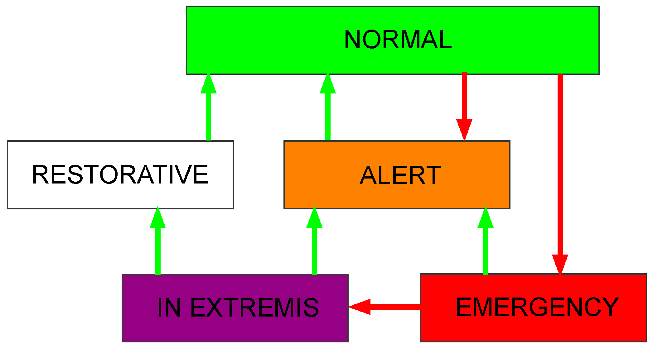
N-1 contingency analysis can be regarded as a part of power system security analysis that is a more general, i.e., wider, concept. In fact, power system security assessment includes other important aspects of security like rotor angle stability, frequency stability and voltage stability, besides N-1 contingency analysis. Thus, security analysis determines the integrity of the power system as well as verification of the power system post-contingency equilibrium state in terms of branch overloads and node voltage deviations.

Most of the time, the power system is in its normal operating state, while contingencies and other system disturbances can lead the system into one of the transient states (Figure 1).

Traditional power system contingency analysis includes numerous power-flow runs with a predetermined list of contingencies. The analysis is also called N-1 security analysis because in every power-flow run the system operates with one component removed from operation (e.g., line, transformer or generator outage). Therefore, obtained node voltages and branch currents are compared with allowable operating limitations. If only one or several limits are hit, the system is characterized as non-secure. Transmission system operators, upon receiving an alert message from the energy management system (EMS), perform remedial actions depending on the type of security threat (line/transformer overload or node voltage outside of admissible limits). The main objective of the remedial action is the improvement of power system security level (e.g., switching of transmission lines, network reconfiguration, phase-shifting transformer action, generation redispatch, etc.). A modern EMS includes power security analysis modules that periodically evaluate the level of power system security and alarm the operator if secure operation of the power system is jeopardized.

The above described methodology is generally performed by application of the Newton–Raphson iterative method for solving the set of nonlinear power-flow equations.

Upon solving the power-flow equations for each contingency, the operating limits are verified for network branches and nodes:

$$I_{i-j}\le I_{i-j\_MAX} \left(\mathrm{for}\mathrm{all}\mathrm{network}\mathrm{branches}\right),$$

$$U_{i\_MIN}\le U_i\le U_{i\_MAX} \left(\mathrm{for}\mathrm{all}\mathrm{network}\mathrm{nodes}\right)$$

where:

• I_i−j is the branch current (line or transformer) and
• U_i is the i-th node voltage.

If the above constraints, for all contingencies, are satisfied, the operating state is said to be N-1 secure.

3. Voltage Stability Analysis

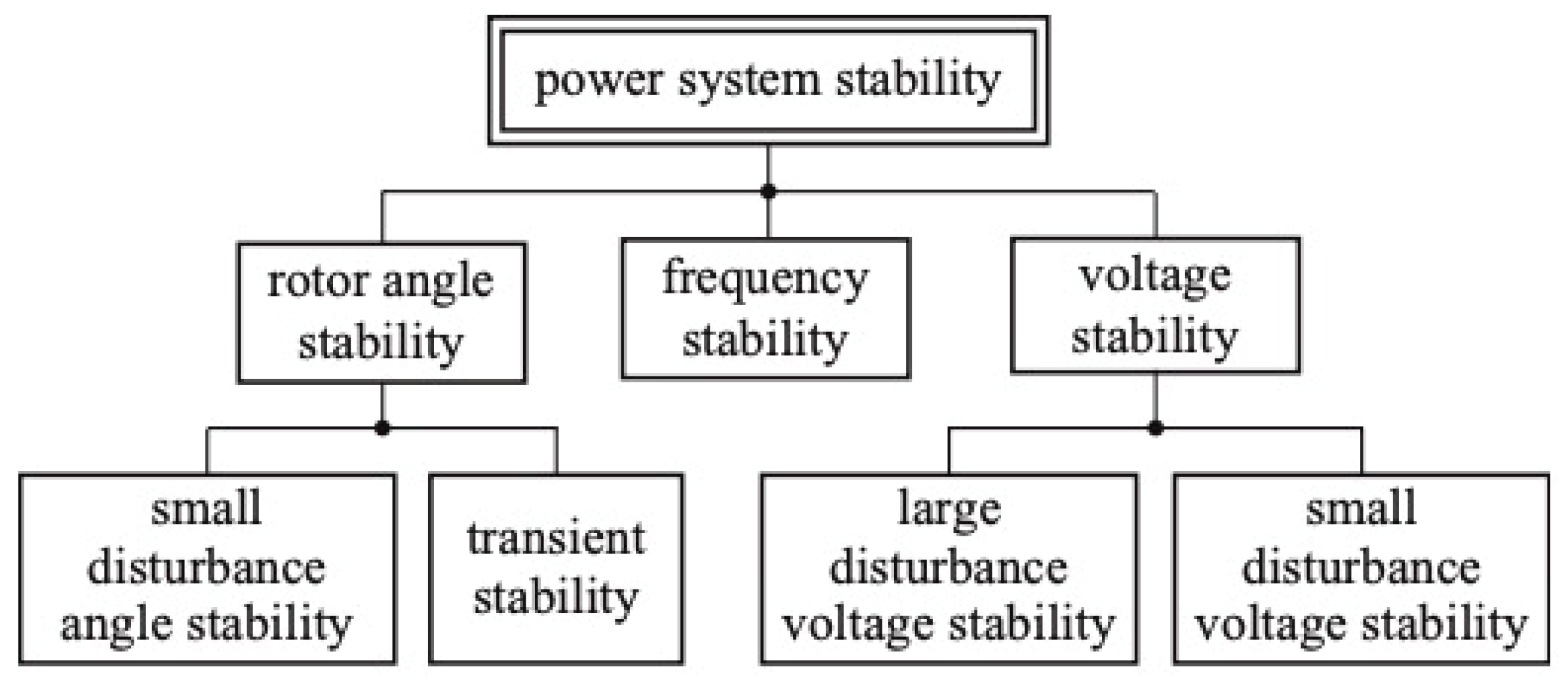
The most general definition of power system stability can be expressed as the ability of the power system to regain a stable operating point after being exposed to a physical disturbance. Voltage angle, magnitude and frequency are the basic quantities necessary to define and classify power system stability. Consequently, power system stability is divided into rotor angle stability, frequency stability and voltage stability.

Due to the nonlinear nature of power systems, a strong dependence on both initial conditions and magnitude of a physical disturbance can be observed. Therefore, a subdivision of power system stability is generally introduced, i.e., small disturbance angle/voltage stability and large disturbance angle/voltage stability.

The generally accepted classification of power system stability is presented in Figure 2.

Small disturbance (signal) voltage stability is concerned with the power system being voltage stable (voltage within acceptable limits) when subjected to small disturbances, e.g., a small increase of system load. Electric load characteristic and continuous and discontinuous control operation (e.g., ULTC operation) can affect small signal voltage stability.

Large disturbance (signal) voltage stability is mainly concerned with power system operation when exposed to large disturbances such as short circuits, generation loss, line tripping and the ability of the system to keep node voltages within prescribed deviations. The response of the system, that is, the ability of the system to remain voltage stable, depends on system characteristics, load characteristics, and the cumulative effect of protection and control devices and systems.

As power systems are being operated closer to equipment rated values, the analysis of voltage stability gains more and more attention. In fact, in the planning and operating stage of the power system, the analysis of voltage stability includes the assessment of two significant aspects, given a system state: (I) proximity to the point of voltage instability and (II) the mechanism by which the instability develops. While the first aspect gives a measure of system security with respect to voltage stability, the second aspect indicates the possible countermeasures to enhance voltage stability.

In fact, one of the most useful method for voltage stability assessment is the well-known concept of modal analysis. However, one must bear in mind that the results obtained by modal analysis are valid for incremental changes only and give information on system state trends rather than actual numerical values, e.g., distance to the point of voltage collapse.

The linearized steady state system power-voltage equations are given by Expression (1), where the Jacobian matrix is the same as the one used for solving the power-flow problem with the Newton–Raphson solution algorithm:

$$\left[\begin{array}{c}∆P\\ ∆Q\end{array}\right]=\left[\begin{array}{cc}{J}_{P\theta }& J_{PV}\\ J_{Q\theta }& J_{QV}\end{array}\right]\left[\begin{array}{c}∆\theta \\ ∆V\end{array}\right],$$

(1)

where:

• ΔP—bus incremental active power change,
• ΔQ—bus incremental reactive power change,
• ΔV—bus incremental voltage magnitude change,
• Δθ—bus incremental voltage phase change.

J_Pθ, J_PV, J_Qθ and J_QV are the active power sensitivity to bus voltage phase change, active power sensitivity to bus voltage magnitude change, reactive power sensitivity to bus voltage phase change, and reactive power sensitivity to bus voltage magnitude change, respectively.

Although voltage stability is affected by both active and reactive power, voltage stability analysis for a fixed operating point can be conducted by considering only changes in reactive power while keeping active power constant. Thus, the effects of active power variations on voltage stability can be considered for different operating conditions (loading levels, power transfers, etc.) again by fixing active power changes and analyzing the incremental relationship between reactive power and voltage.

If active power is kept constant (similar to traditional Q-V curve analyses), the previous equation can be reduced to, [37]:

$$∆Q=\left[J_{QV}-J_{Q\theta }·J_{P\theta }{}^{-1}·J_{PV}\right]∆V=J_R·∆V,$$

(2)

with:

$$J_R=\left[J_{QV}-J_{Q\theta }·J_{P\theta }{}^{-1}·J_{PV}\right].$$

J_R is called the reduced Jacobian matrix of the system and directly relates bus voltage magnitude with reactive power injection.

Performing eigenvalue analysis on the matrix J_R, eigenvalues ${\lambda }_i$ and the corresponding right and left eigenvectors are obtained. In fact, the eigenvalues and the right and left eigenvectors, similar to the concepts used in dynamic system analysis, define the modes of voltage instability. However, contrary to the concepts common in angle stability analysis, the smaller the size of an eigenvalue, the weaker the corresponding modal voltage. If a voltage mode eigenvalue equals zero it is a clear indication of imminent voltage collapse because any variation in modal reactive power will cause infinite modal voltage variation. If, however, an eigenvalue has a negative value it indicates that the system has passed the critical point of voltage stability. Therefore, the values of the eigenvalues indicate the modes (areas) that are most prone to voltage instability (modes with the smallest eigenvalues). However, the value of an eigenvalue itself is not a quantitative indicator, it is only a “warning signal” that has to be further “investigated” by proper analysis, as per the proposed methodology given in Section 5.

Branch and generator participation factors are calculated from the modal eigenvectors and give particularly valuable information on possible remedial actions in cases of voltage stability issues. In fact, branch participation factors indicate, for each mode, branches that consume large amounts of reactive power for incremental changes in reactive loading and cause a particular mode to be weak, i.e., susceptible to voltage instability.

Branch l-k participation factor to mode i is calculated from Equation (3):

$$P_{l-k\_i}=\frac{∆Q_{l-k\_i}}{∆Q_{l\_max\_i}},$$

(3)

while generator’s k participation factor to mode i is calculated from Equation (4):

$$P_{g\_i}=\frac{∆Q_{g\_i}}{∆Q_{g\_max\_i}}.$$

(4)

On the other hand, generator participation factors indicate, for each mode, which generators supply the most reactive power in response to an incremental rise in system reactive loading. Generators with high participation for particular modes are critical for maintaining the stability of such modes.

In the above Equations (3) and (4) ΔQ_{l_max_i} is the maximum incremental change of reactive loading on line l-k for all the modes, and ΔQ_{g_max_i} is the maximum incremental change of reactive power variation on generator g for all the modes, ΔQ_{l−k_i} is the incremental change of reactive power loss on line l-k for mode i, and ΔQ_{g_i} is the incremental change of reactive power variation on generator g for mode i.

4. Reactive Power Resources and the Effect of Load Modeling on Voltage Stability

Since the problem of voltage stability is strongly linked to the local deficiency in reactive power support, the next subsections give a brief overview of some traditional and modern reactive power resources.

4.1. Synchronous Generators

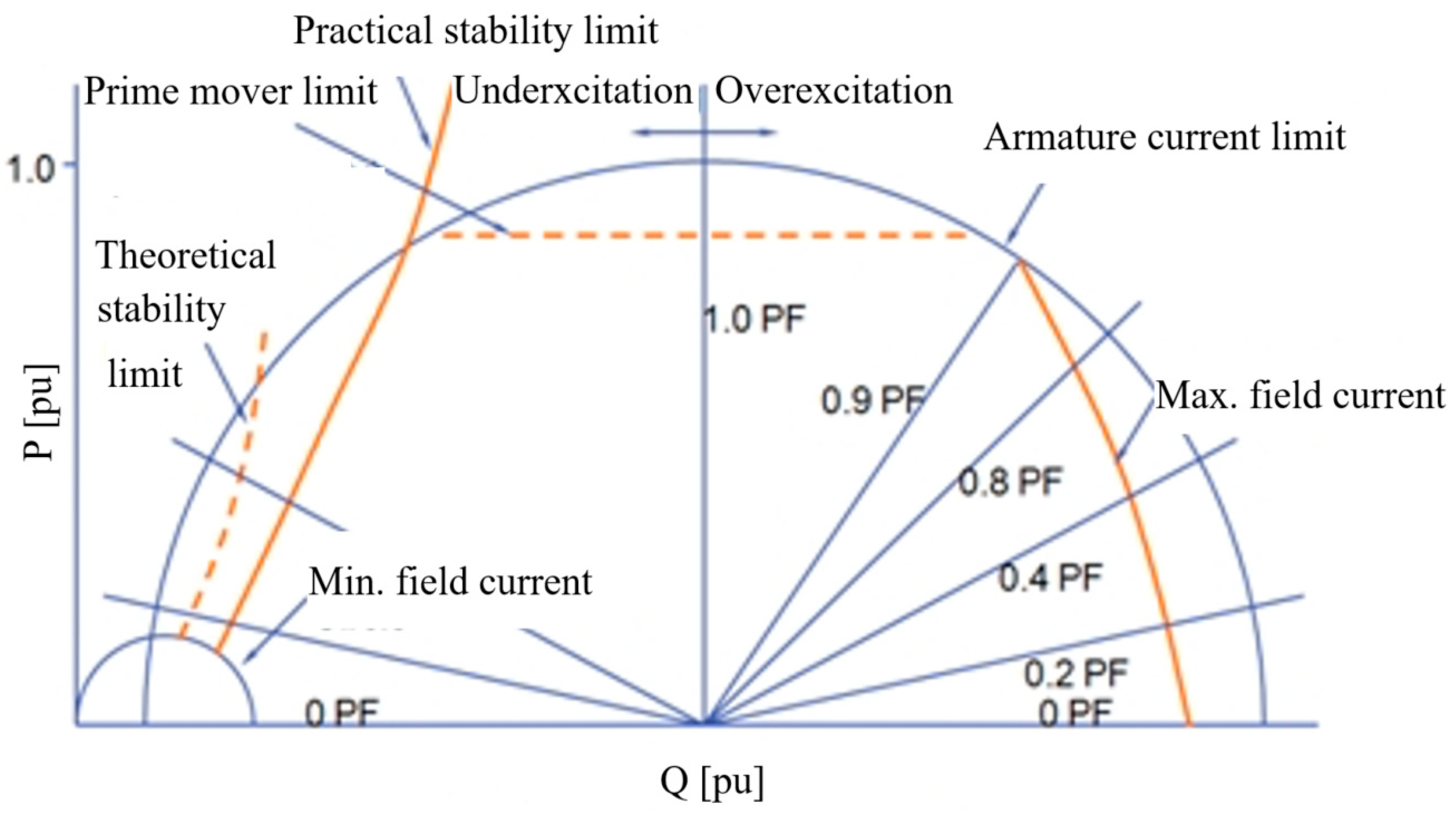
The operating region within which the synchronous generator (SG) can operate safely is called the capability curve (Figure 3). Capability curves, provided by manufacturers, are used to optimally exploit synchronous machines during their lifetime. In fact, protection systems based on capability curves safeguard the machine from being thermally overloaded or operated near static/dynamic stability limits. As shown in Figure 3, capability curves are usually given in the P-Q plane where the most important limitations are plotted—stator and rotor current limits, static and dynamic stability limits and thermal restrictions [38]. As SGs are the most valuable sources of reactive power in the power systems they are often operated in the overexcited region, thus having only a limited amount of reactive reserve capability.

4.2. Distributed Energy Resources (DERs)

Distributed energy resources, due to their vicinity to consumption centers, are more and more taken into consideration when searching for sources of reactive power and tools for voltage problem mitigation [39]. In fact, inverters already present in PV installations, are one of the key elements of future power grids. DERs can provide both active and reactive power, therefore they can be used to provide ancillary services to the system operator, e.g., voltage and/or frequency regulation. Although the number of PV plants is increasing rapidly, exploitation of PV inverter full capabilities is still low [40].

In the case of reactive power, the grid codes require that large-scale PV power plants inject or absorb reactive power according to a predefined relationship between the active and reactive power or a specific value of reactive power. In [41] the authors presented active and reactive power control of a PV generator for grid code compliance.

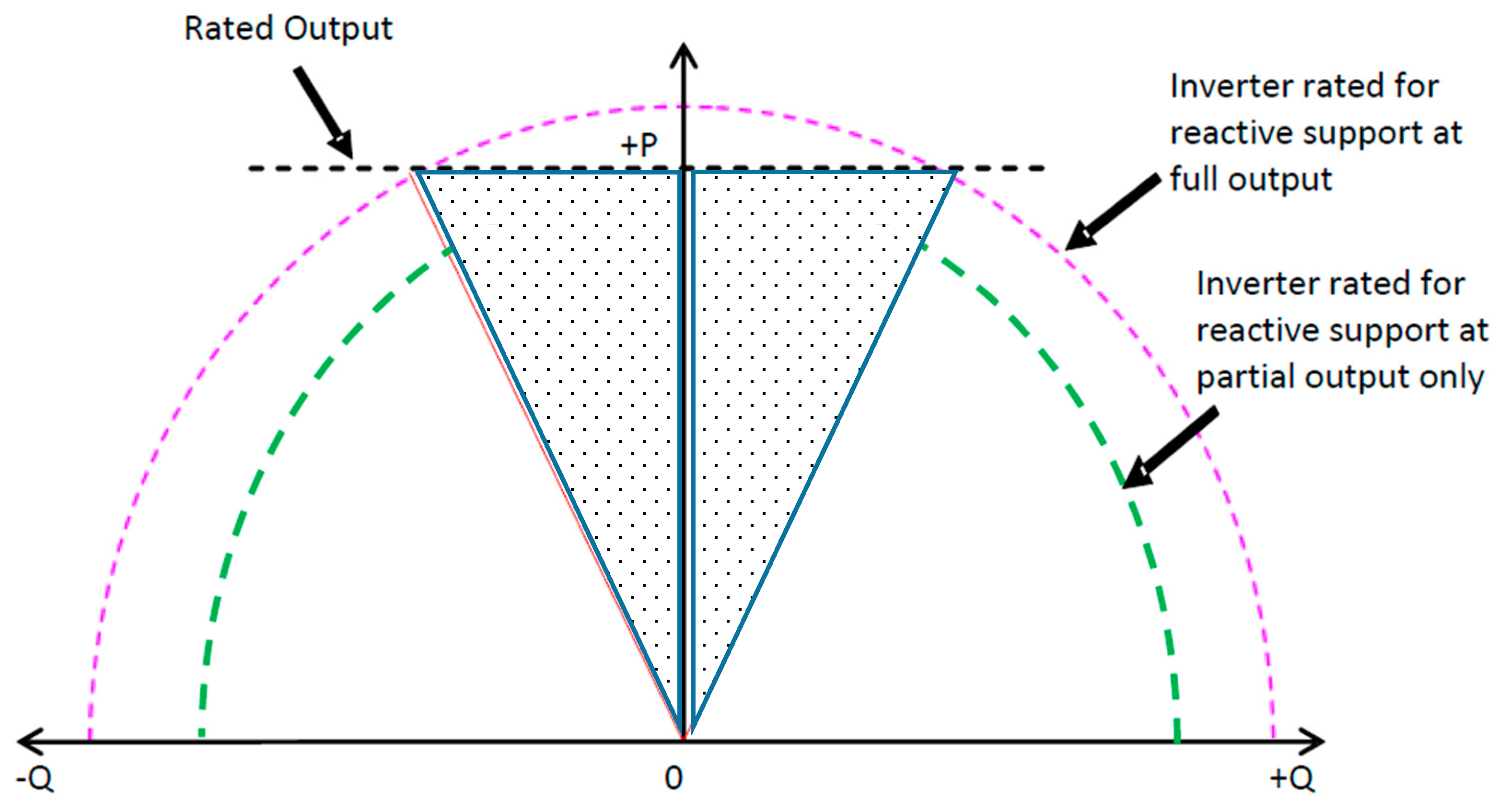
Grid-connected PV installations usually operate at unity power factor over their entire active power output range, thus providing no reactive power support to the grid [42]. Most small-scale PV inverters for residential and commercial applications are not designed to provide any reactive power at nominal power output. Conversely, large-scale PV installations can usually provide similar reactive power support at full and partial output. Of course, reactive power output at lower active power levels can be considerably higher than at higher active power levels, depending on the inverter’s thermal limitations and voltage at the connection point. The inverter’s capability curves differ considerably from those presented in Section 4.1. Since inverters are designed to operate only within voltage deviations of ±10% of rated terminal voltage, obviously their reactive power capability is greatly affected by distribution grid voltage fluctuation. For instance, when the terminal voltage reaches the upper limit no additional reactive power can be provided [42].

Some interconnection standards reviewed in [43,44], applicable to large-scale transmission-connected PV plants, describe reactive capability requirements as “triangular,” “rectangular” or with a similar reactive capability characteristic, as presented in Figure 4.

4.3. Battery Energy Storage Systems

Battery energy storage systems (BESSs) achieve energy storing by electro-chemical conversion. When charged, BESSs convert electrical energy into chemical, which is eventually converted back into electricity when the BESS discharges. Since BESSs incorporate both an energy storage unit and a voltage source converter, separate control of active and reactive power injection into the grid can be realized [45].

BESSs can respond quickly to control signals, thus providing fast power ramping functions with accurate control. In fact, BESSs installed in active distribution systems can provide smoothing of power fluctuations and deliver valuable ancillary services to the distribution system operator (DSO), e.g., frequency regulation and peak load shaving and/or shifting. When installed in medium and low voltage distribution networks, BESSs can provide reactive power support [46].

A further application of BESSs is expected, as more and more BESSs are installed at transmission system level (high and extra high voltage). In fact, transmission system operators (TSO) can benefit from emergency power from BESSs, black-start service (reenergizing and island operation), and supply and demand leveling in systems with a high share of renewable power (solar and wind) [47].

Since BESSs are interfaced with the rest of the power system through similar power electronic devices/inverters as, e.g., PV systems, the simulation results presented in the following sections are identical to the results obtained for distributed energy resources. However, it must be emphasized that BESSs as providers of flexibility to the power system are in a different position, compared to distributed generators, which are mainly concerned with maximization of active power production.

4.4. Regulation Transformers (Under Load Tap Changers—ULTCs)

Power transformers that connect transmission networks with distribution networks are predominantly equipped with ULTCs, which allow voltage regulation under load. Automatic voltage regulators associated with ULTCs are responsible for maintaining nearly constant voltage on the secondaries of distribution power transformers, irrespective of load variation. In some cases, the line drop compensation (LDC) function is used that allows voltage drop along distribution lines to be effectively compensated. However, when DERs are installed at the secondaries of distribution transformers, line drop compensation cannot be applied.

The self-regulation of the ULTC transformation ratio is an important factor causing voltage instability. In fact, for different system operating conditions, different load types and different transformation ratios, the voltage-regulating effect may be different [48].

Besides ULTC operation, voltage dependence of the loads and synchronous generators reaching over-excitation limits are considered as the three most influential factors leading to voltage instability [49].

4.5. Electric Load Composition

In recent years electric load modeling has once again gained much attention owing to the renewable energy source integration, demand-side management smart metering devices, etc.

However, the importance of load modeling and its influence on system voltage stability is well known. In fact, T. J. Overbye, back in 1994, explored the effects of load modeling on power system voltage stability analysis and determined that the type of model used to represent loads has a tremendous effect upon the assessment of system voltage stability [50].

More recently, in [51] the authors presented a comprehensive review of load modeling and identification techniques (measurement-based and component-based).

In [52] the authors demonstrated the procedure of dynamic load modeling by using real-world measurements. To capture, i.e., record load dynamics, voltage perturbations were introduced by altering tap settings on the transformer ULTC, thus changing the voltage on the secondary (load) side.

Vignesh et al. in [53] demonstrated the potential to significantly improve existing load modeling practice by phasor measurement units (PMUs).

Load models, depending on the type of analysis, are of the static or dynamic type. Static models express the active and reactive power as functions of bus voltage magnitudes and frequency and are constant in time. On the other hand, dynamic models express the active and reactive powers as a function of voltage and time [51].

In our research the commonly used ZIP model in both steady state and dynamic studies was adopted. The ZIP model represents the relationship between the voltage magnitude and power in a polynomial equation that combines constant impedance (Z), current (I), and power (P) components:

$$P_L=P_0\left[{\alpha }_Z{\left(\frac{V_L}{V_0}\right)}^2+{\alpha }_I\left(\frac{V_L}{V_0}\right)+{\alpha }_P\right],$$

(5)

$$Q_L=Q_0\left[{\beta }_Z{\left(\frac{V_L}{V_0}\right)}^2+{\beta }_I\left(\frac{V_L}{V_0}\right)+{\beta }_P\right]$$

(6)

where:

• P_L is the actual active load power,
• Q_L is the actual reactive load power,
• P₀ is the base value of active load power at nominal voltage,
• Q₀ is the base value of reactive load power at nominal voltage,
• V₀ is the nominal voltage,
• V_L is the actual voltage,
• α_Z, α_I, α_P are the proportion of constant impedance load, constant current load and constant power load for real power, respectively. β_Z, β_I and β_P are similar quantities for reactive power.

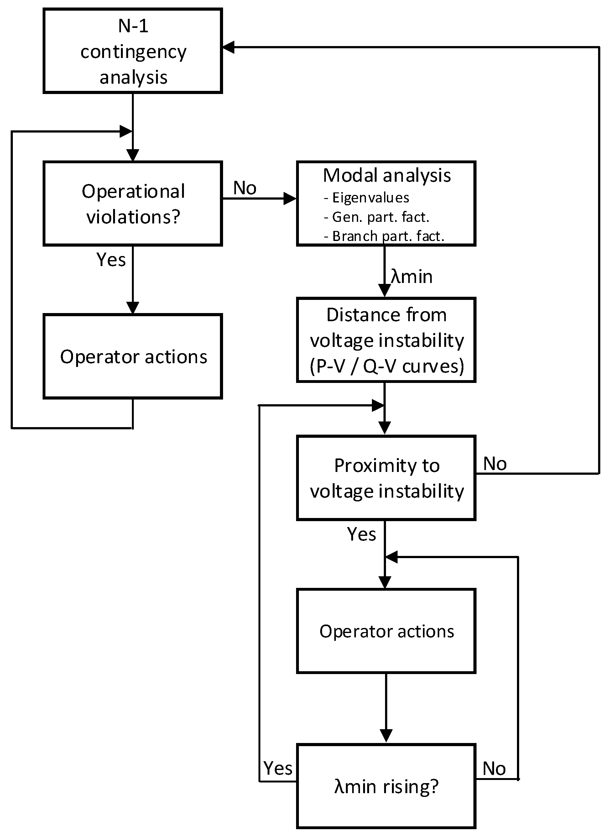
5. Extended Contingency Analysis

In this section, the concept and practical realization of the extended power system N-1 contingency analysis is explained. In fact, combining the previous concepts of N-1 contingency analysis and modal analysis for voltage stability, enhanced with predetermined priority lists based on eigenvalue sensitivity analysis, an enhanced contingency analysis tool can be realized.

In the first step a classic N-1 contingency analysis is performed to determine possible element overloading and/or unallowable voltage deviations. After every run of the power flow, modal analysis of voltage stability is performed to record the corresponding eigenvalues.

If, during contingency analysis, operating limit violations are detected, remedial actions must be performed to keep the desired level of power system security. Thus, for every remedial action at hand, voltage stability modal analysis is performed, and the corresponding eigenvalues are recorded. By comparison of the eigenvalues, the system operator dispenses valuable information regarding voltage stability. On the other hand, if no violations of operating limits are recorded, obtained results could in some cases indicate voltage-endangered areas of the power system.

If any of the calculated eigenvalues becomes very small, i.e., close to zero, the corresponding generator and branch participation factors are determined, thus indicating which generators are the most influential to voltage stability enhancement and which branches consume the most reactive power for the simulated case.

Finally, for the most critical voltage stability modes, active and reactive power loading limits are calculated as possibly the most valuable information for the system operator to keep the power system stable in terms of voltage stability.

The proposed algorithm is given in Figure 5 as a flow diagram.

Operator actions (remedial action schemes) provided for overloads and/or voltage violations mitigation are determined in advance for a selected number of contingencies and operating scenarios (e.g., for various loading levels, network topologies, unit commitment, renewable energy sources generation, etc.). Also, operator actions provided for voltage stability enhancement are also performed in advance and organized as priority lists. Fast ranking of operator actions is done through calculation of the voltage-based performance index PI_V [24]:

$$P{I}_V={\displaystyle \sum }_i^n\frac{w_i}{2\alpha }{\left(\frac{\left|V_i\right|-\left|V_i^r\right|}{∆V_i^{lim}}\right)}^{2\alpha }$$

(7)

where:

• $\left|V_i\right|$—voltage magnitude at bus i,
• $\left|V_i^r\right|$—rated voltage magnitude at bus i,
• $∆V_i^{lim}$—voltage deviation limit, above which voltage deviations are unacceptable,
• n—number of buses in the system,
• w_i—real non-negative weighting factor to give higher weights to critical buses,
• α—exponent of penalty function (α = 1 preferred).

Therefore, in the next section analysis of the countermeasures against voltage instability is performed to prioritize the countermeasures and to evaluate and compare the benefit of “classic” (synchronous generators and regulation transformers) and “new” (distributed energy sources, energy storage) resources. In addition, special attention was given to the load modeling aspect as a key factor influencing the perception of the voltage stability/instability margin.

The following section presents the model of the western part of Croatia’s 110 kV transmission system and the most important results of the performed simulations. Special emphasis was given to

• reactive power capability of distributed generation,
• energy storage reactive capability,
• synchronous generators reactive capability, and
• regulation transformer action.

After exploring the influence of the aforementioned resources on voltage stability enhancement the critical impact of load modeling was investigated.

6. Simulations

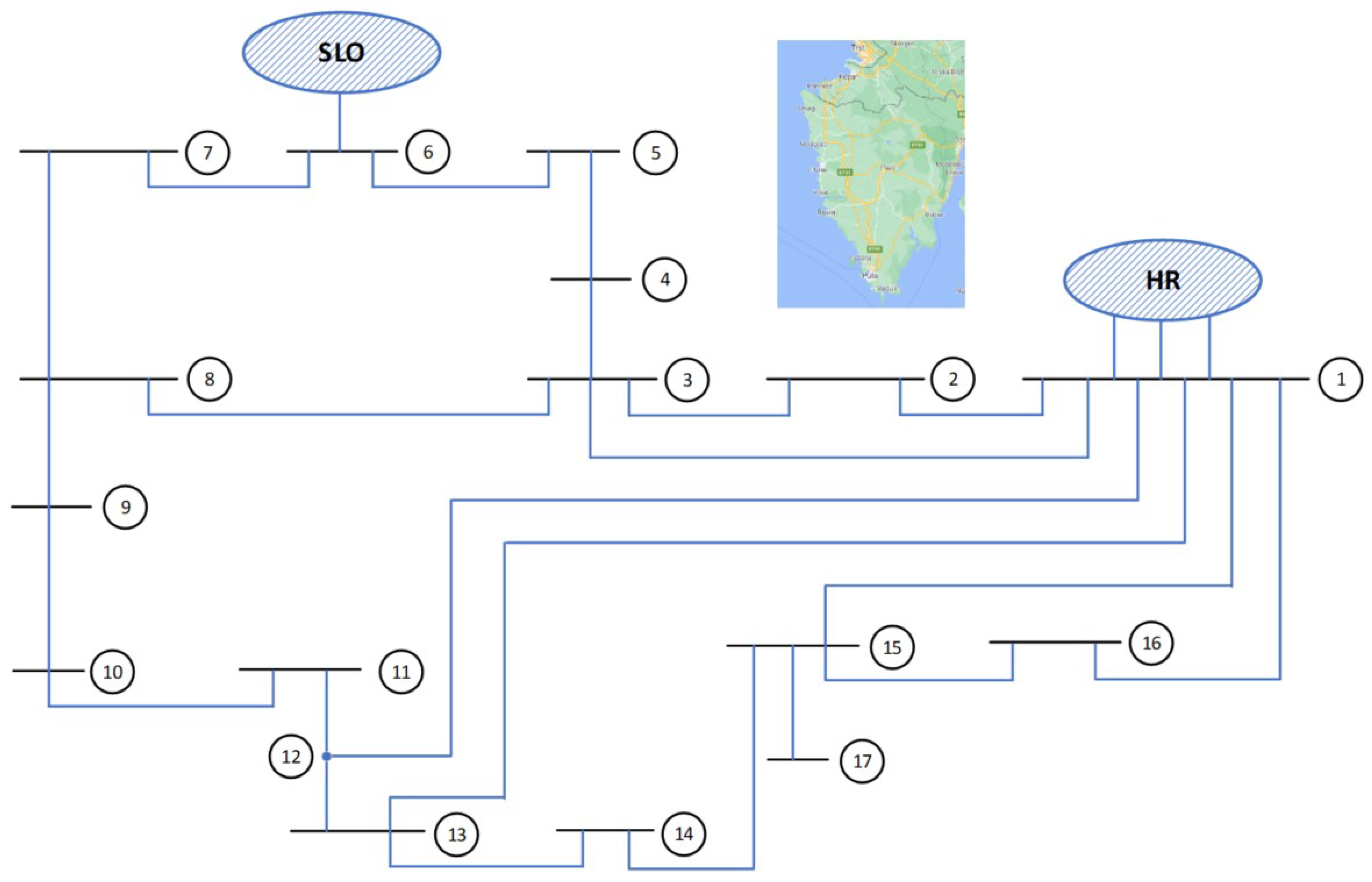
Research was performed on a simulation model representing the western part of Croatia’s 110 kV transmission power system, including interconnecting transmission lines to the Slovenian power system and the rest of the Croatian power system (Figure 6). The modeled power system parameters (branch impedances and bus loading) are given in the Appendix A. All simulations were carried out using Neplan Electricity software on a personal computer.

The loading in the simulated scenario was high and corresponded to the summer peak loading achieved on 10 August 2019 in the 20th hour. The total load of 270 MW and 23 Mvar was distributed among 16 load-type nodes with one generator node producing 200 MW and 13 Mvar connected at bus 1. Loads were fed through transformers with under load tap changers (ULTCs). For the purpose of simulation and determination of voltage collapse countermeasures, at buses 5, 8 and 11 battery storage systems/PV plants were connected. N-1 contingencies included all 110 kV transmission lines, generator outage at node 1 and interconnection line outage.

Simulations were performed in the following order: first, in the normal operating condition when all network elements were available, the modal analysis was performed and the P-V and Q-V curves were determined for the weakest mode, i.e., for buses with high participation factor in the weakest mode (smallest eigenvalue). Accordingly, the distance from the current operating point to the critical point on the P-V and/or Q-V curve was calculated and compared with the adopted safety margin. The same procedure was then performed for the assumed contingencies.

Afterwards, simulations necessary for ranking of the considered countermeasures against voltage instability (eigenvalue sensitivity with respect to reactive power capability of synchronous generators, distributed generation/energy, regulation transformer action) were performed and the voltage-based performance index (Equation (7)) calculated.

Finally, the effect of load modeling, i.e., load composition on voltage stability, was further investigated in later simulations.

7. Results and Discussion

As previously described, many simulations were carried out to investigate the appropriateness of the proposed methodology for ECA, including remedial action ranking.

Table 1. Eigenvalues corresponding to weakest mode in each simulated contingency.

Contingency Number	Contingency (Line or Generator)	λ1 [-]	Mode 1 Area (Bus)
0	Base case (N-0)	0.416	6–7
1	3–4, L	0.325	5
2	1–11–13, L	0.335	11
3	4–5, L	0.348	5
4	8–3, L	0.353	8–9
5	1–3, L	0.355	6–7
6	1–2, L	0.356	6–7
7	2–3, L	0.366	6–7
8	1, G	0.368	6–7
9	10–11, L	0.376	10
10	5–6, L	0.390	6
11	7–8, L	0.397	7
12	1–13, L	0.403	6–7
13	8–9, L	0.405	9
14	14–15, L	0.405	6–7
15	6–7, L	0.411	6–7
16	9–10, L	0.411	6–7
17	1–15, L	0.412	6–7
18	13–14, L	0.415	6–7

presents the results of the modal analysis (eigenvalue of the first weakest mode and indication of the area belonging to it) for the base case (N-0) and for all simulated contingencies (N-1).

By inspection of the previous table it is clear that most contingencies caused voltage stability problems in the same area (buses 6 and 7). Also, from contingency number 15 and onward the eigenvalues were very similar to the eigenvalue of the base case, thus indicating that these contingencies did not change the operating conditions in relation to voltage stability. For contingencies that included outage of elements interconnecting the analyzed area with the rest of the system (network transformers 220/110 kV, interconnection lines 110 kV and 220 kV), the results were comparable with contingency numbers 2 and 7, respectively.

Taking into consideration the results presented in Table 1, P-V curves and Q-V curves were determined for the nodes belonging to the weakest modes for each contingency, (e.g., for contingency No. 3, P-V and Q-V curves were determined only for node 5). Having at hand P-V and Q-V curves and predetermined safety margins, the distance from the critical operating point was calculated.

Table 2. Voltage stability indicators for the base case and the most severe contingency.

Scenario	λmin [-]	Mode Area (Bus)	Bus No./ΔPcrit [-]/[%] *	Bus No./ΔQcrit [-]/[Mvar]	Bus No./U-Qmax [-]/[%/Mvar]
Base case	0.416	6 and 7	6/>87	6/87.6	6/0.17
			7/>83	7/85.5	7/0.17
No. 1 (most severe)	0.325	5	5/>72	5/41.3	5/0.36
No. 18 (least severe)	0.415	6 and 7	6/>88	6/87.9	6/0.17
			7/>84	7/85.6	7/0.17

* Percentage increase in relation to base load given in Table A2 of the Appendix A.

presents the results obtained following the previously described methodology for the base case scenario, when all lines and transformers were available, and for the N-1 scenario that resulted with the smallest eigenvalue (λ_min), indicating a possible voltage instability area. Although the second column of Table 2 indicates the mode with the smallest eigenvalue (λ_min), this value alone does not tell the system operator how close the system is to voltage instability. The most valuable information is given to the system operator in columns three and four, resulting from inspection of calculated P-V and Q-V curves for buses belonging to the weakest mode. Actually, the third and fourth column explicitly give the absolute distance of a specific node (bus) from the point of voltage instability in terms of possible active and reactive loading increase, respectively. The last column confirms qualitatively what columns three and four express quantitatively, i.e., column five gives the voltage sensitivity factor of bus nodes to bus reactive power injection and thus indicates the “weakest” nodes in terms of voltage stability but gives no information on how close the system to voltage instability is.

Hence, performing modal analysis for the considered subsystem and subsequent analysis of the corresponding P-V and Q-V curves for only the weakest mode gives the operator a fast and reliable indication of problematic areas of the power system. However, even with this information at hand, the system operator has little insight on what are the best countermeasures, i.e., remedial actions for increasing voltage stability indicators.

In fact, for the system operator to be able to make immediate decisions, the ranking of the countermeasures against voltage instability must be known in advance. Since the operating conditions—loading, network topology, unit commitment, distributed resources availability—constantly change, a large number of offline simulations have to be performed, along with the ranking of countermeasures carried out for each scenario, as demonstrated in the next section for the maximum loading scenario.

7.1. Distributed Energy Resources/Battery Energy Storage (DER/BES)

To determine the beneficial impact on voltage stability, at nodes 5, 8 and 11 distributed generators were connected, all with the same characteristics (nominal power 10 MVA, power factor 0–1.0). Although simulations were conducted for all considered contingencies, in the following text results are presented for one selected contingency, i.e., contingency No. 7 (outage of lines 2–3). Throughout every contingency case consideration, the voltage-based performance index was calculated alongside the corresponding P-V and Q-V curves. Remedial actions that were herein considered were the changes of the operating point of DER/BES systems, i.e., switching from maximum active power production (assuming the availability of the renewable resource and the adequate state of charge of the BES) to maximum reactive power production (assuming there is a compensation for DER/BES reactive power support to the system operator). Thus, the DER/BES enters in the so-called VAR mode of operation (reactive mode), injecting the largest possible value of Mvars, i.e., operating with the lowest possible power factor.

Table 3. Voltage stability indicators and ranking of remedial actions (distributed energy resources/battery energy storage, DER/BSS) for contingency No. 7.

Remedial Action Number	Remedial Action	λnew/λold [-]	ΔP System * [%]	ΔQ at Bus 6 [Mvar]	PIV [-]
0	5Pmax, 8Pmax, 11Pmax	1.000	72	71.4	0.399
1	5Qmax, 8Pmax, 11Pmax	1.027	75	76.6	0.227
2	5Pmax, 8Qmax, 11Pmax	1.025	75	75.2	0.202
3	5Pmax, 8Pmax, 11Qmax	1.016	73	73.7	0.228
4	5Qmax, 8Qmax, 11Pmax	1.049	78	80.5	0.189
5	5Qmax, 8Pmax, 11Qmax	1.041	77	79.2	0.175
6	5Pmax, 8Qmax, 11Qmax	1.038	76	77.7	0.148
7	5Qmax, 8Qmax, 11Qmax	1.062	79	83.1	0.251

* Percentage increase in relation to base load given in Table A2 of the Appendix A.

summarizes simulation results needed to perform remedial action ranking. In fact, the second column of Table 3 defines the remedial action (e.g., 5_Qmax, 8_Pmax, 11_Pmax means the operating point of the DER/BES connected at node 5 was changed from maximum active production to maximum reactive production, while the DER/BES connected at nodes 8 and 11 remains in maximum active power production regime). The third column demonstrates the increase of the corresponding eigenvalue, indicating the moving of the system away from voltage instability. Columns four and five give the allowable increase in active and reactive loading before reaching the critical point on the bus most prone to voltage instability (column four gives the percentage value of the overall active power increase from the base scenario, while column five presents the maximum possible reactive power increase for the selected node). Finally, column six gives the PIV index calculated by (7), which is used for ranking of the considered remedial actions. Of course, the ranking of remedial actions can consider other indices based on, e.g., ΔP or ΔQ, or some other combination as in [24].

By inspection of Table 3 we can conclude that remedial action No. 6 gives the best result, considering overall voltage deviations in the analyzed subsystem with a possible increase of overall network active loading by 76% and 77.7 Mvar reactive loading at the critical bus No. 6 before voltage collapse occurs. Remedial action No. 0 means that no remedial action is undertaken.

7.2. Synchronous Generators (SGs)

To compare the effect of reactive power injection on voltage stability from synchronous generators and rank the remedial actions with previously considered reactive energy sources, three simulation scenarios for the same contingency (No. 7) were analyzed—the reactive power output from the SG connected at node 1 was discretely increased as to mimic reactive power production of DER units connected at nodes 5, 8 and 11. The results are presented in

Table 4. Voltage stability indicators and ranking of remedial actions (synchronous generator, SG) for contingency No. 7.

Remedial Action Number	Remedial Action	λnew/λold [-]	ΔP System * [%]	ΔQ at Bus 6 [Mvar]	PIV [-]
0	QSG = 41 Mvar	1.000	72	71.4	0.399
1	QSG = 51 Mvar	1.005	72	72.3	0.327
2	QSG = 61 Mvar	1.008	72	72.7	0.283
3	QSG = 71 Mvar	1.011	72	72.7	0.242

* Percentage increase in relation to base load given in Table A2 of the Appendix A.

.

In the first analyzed case (remedial action No. 1) the base reactive power output of the SG connected at node 1 was increased by 10 Mvar, which corresponded to the case when a DER/BES unit connected at one of the nodes 5, 8 or 11 generated the same amount of reactive powers. By inspection of Table 4 it follows that increasing reactive power output at node 1 improved slightly the voltage stability indicator (λ_new/λ_new) and the possibility to increase reactive loading at the critical bus No. 6. The voltage-based performance index decreased as the voltage deviations in the analyzed subsystem also decreased with higher injection of reactive power in node 1. The overall active power loading of the analyzed subsystem remained unchanged. In the remaining two cases the reactive power output at node 1 was further increased by 10 and 20 Mvar, respectively. The results were similar to the ones in the first case, thus suggesting the inappropriateness of the considered countermeasure against voltage instability, compared to the previously considered remedial actions.

7.3. Regulation Transformers

Different regulation transformer action strategies were analyzed to evaluate their possible contribution to voltage stability enhancement. The first case explored the influence of blocking automatic voltage regulators (AVR) in neutral position, while the second case examined blocking of AVRs in the position just before the N-1 contingency occurs. Therefore, the corresponding indicators were calculated, and the results presented in

Table 5. Voltage stability indicators and ranking of remedial actions (under load tap changer, ULTC) for contingency No. 7.

Remedial Action Number	Remedial Action	λnew/λold [-]	ΔP System * [%]	ΔQ at Bus 6 [Mvar]	PIV [-]
0	AVR in normal operation	1.000	72	71.4	0.399
1	AVR blocked in neutral position	1.003	86	77.0	0.302
2	AVR blocked in optimum position before contingency	1.003	81	75.5	0.378

* Percentage increase in relation to base load given in Table A2 of the Appendix A.

. The two cases can be compared to the case when the AVRs were left in operation, thus trying to maintain secondary voltage as close to the nominal value (second row of Table 5).

By examination of the previous table it is clear that setting and then blocking the tap changers in neutral position slightly enhances voltage stability, thus moving the operation point away from voltage stability limits in terms of both active and reactive loading. However, looking at the voltage-based performance index, it is again deducible that remedial action schemes that included sources of reactive power electrically close to critical areas of the power system in terms of voltage stability, are the preferred choice for the system operator.

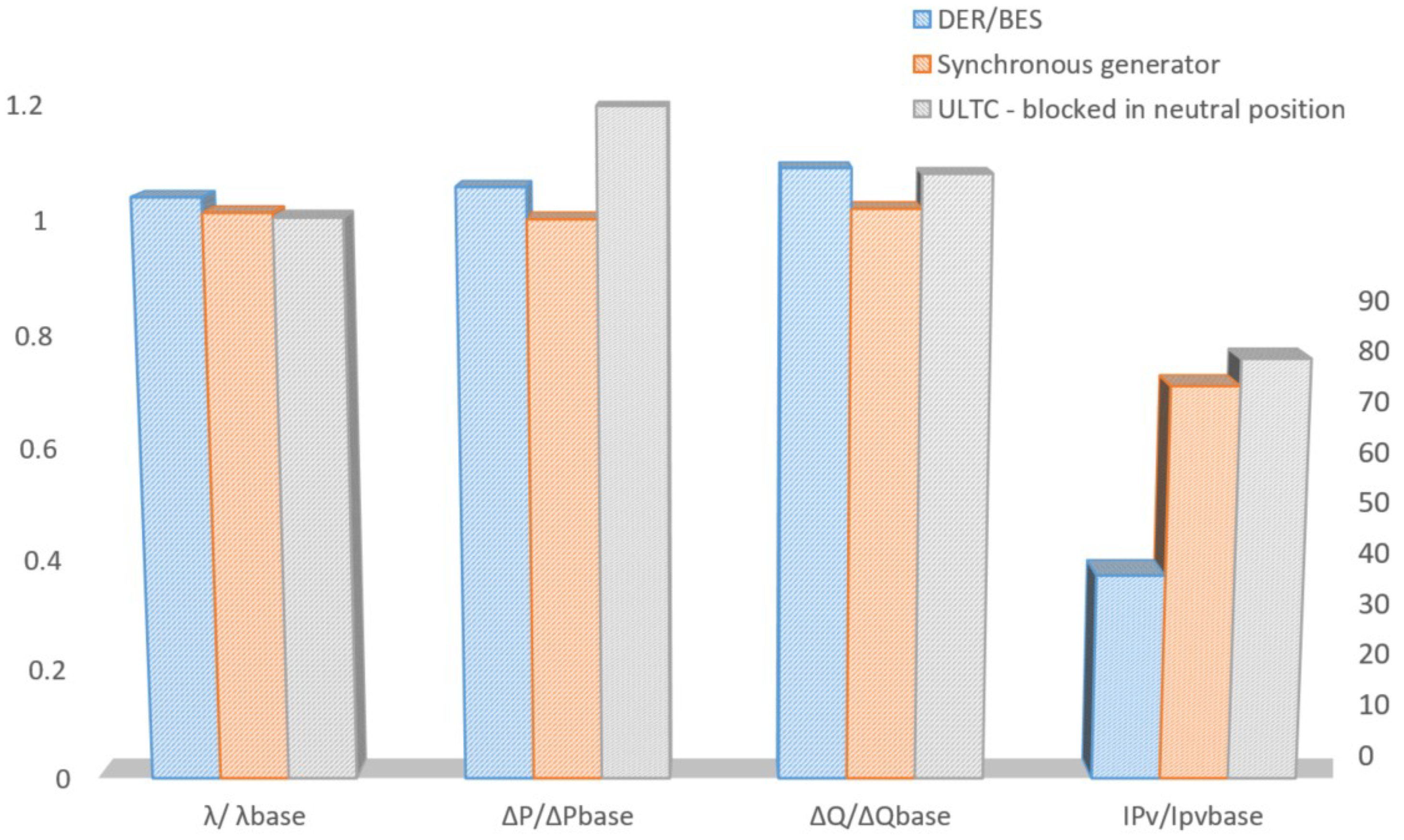
Figure 7 presents a direct comparison of different type remedial actions based on DER/BES, synchronous generators and ULTC and its effects on voltage stability indicators for the analyzed power system (the values are normalized with results for the base case). The chart was constructed based on data given in Table 3, Table 4 and Table 5. The picture shows the priority and the effects of the countermeasures at hand for the system operator.

Although blocking of the AVRs in neutral position might seem an attractive measure for voltage stability increase, its effect on the overall voltage deviation was disadvantageous, as can be seen from the value of the voltage-based performance indicator, not to mention the long time to perform such a measure and the wear and tear of the tap changers. Increasing reactive power production on large synchronous generators, electrically distant from the critical buses, proved also to be inferior to the DER/BES located strategically in the system.

7.4. Load Modeling Effects on Voltage Stability Analysis

The influence of the load-type model (variation of tip ZIP parameters) was analyzed by simulation and the results are presented in

Table 6. Voltage stability indices for different load composition types connected at node 7.

BASE CASE ZIP Model Parameters	λmin [-]	ΔPcrit [%]	ΔQcrit [Mvar]	U-Qmax [%/Mvar]
PZIP: 33%/33%/33%	0.414	>87	>87.5	0.17
QZIP: 33%/33%/33%
PZIP: 50%/0%/50%	0.414	>87	>87.5	0.17
QZIP: 50%/0%/50%
PZIP: 0%/0%/100%	0.407	>85	>86.9	0.17
QZIP: 0%/0%/100%
PZIP: 100%/0%/0%	0.421	>88	>88.0	0.16
QZIP: 100%/0%/0%
N-1 CASE No. 7 ZIP Model Parameters
PZIP: 33%/33%/33%	0.365	>72	>71.3	0.20
QZIP: 33%/33%/33%
PZIP: 50%/0%/50%	0.364	>72	>71.3	0.19
QZIP: 50%/0%/50%
PZIP: 0%/0%/100%	0.357	>71	>70.6	0.20
QZIP: 0%/0%/100%
PZIP: 100%/0%/0%	0.372	>74	>71.8	0.19
QZIP: 100%/0%/0%

. ZIP model parameters were varied only for a single load-type bus of the analyzed subsystem, namely, bus No. 6. The simulations were performed for the base case scenario and for the contingency case No. 7.

As expected, the load composition considerably affected voltage stability. Simulations conducted with loads modeled as pure “constant impedance” showed the largest resilience to voltage stability problems, as the loads exhibited an inherent “natural” unloading characteristic. On the other hand, simulations performed with loads modeled as pure “constant power” resulted in considerably unfavorable conditions, both in terms of active and reactive power. It is therefore of great importance to dispose with reliable load models, since over or under estimation of a certain load-type component can result in too optimistic or too pessimistic power system operation limits.

8. Conclusions

Modern power systems are experiencing rapid changes and are continuously exposed to different sources of stress (e.g., high power production of newly connected energy sources such as wind power and/or solar power without corresponding load; areas with large loads and no power production connected to the system through weak links, etc.). Control of power systems in such circumstances becomes considerably challenging. Therefore, in situations when contingencies endanger power system operation, every tool at hand to transmission system operators constitutes a valuable asset. With this in mind, the authors presented a dedicated methodology for enhancement of the classic CA with voltage stability modal analysis, thus achieving the so-called enhanced contingency analysis as a useful transmission system operator tool. The first step of the proposed methodology is the traditional N-1 contingency analysis, which is performed to determine possible element overloading and/or unallowable voltage deviations. If, during contingency analysis, operating limit violations are detected, remedial actions must be performed to keep the desired level of power system security. Thus, for every remedial action at hand, voltage stability modal analysis is performed, and the corresponding eigenvalues are recorded. By comparison of the eigenvalues, the system operator dispenses valuable information regarding voltage stability. On the other hand, if no violations of operating limits are recorded, obtained results could in some cases indicate voltage-endangered areas of the power system.

For the most critical voltage stability modes (i.e., modes with smallest eigenvalues), active and reactive power loading limits are determined (from P-V and Q-V curves), which are of the most interest to the system operator in charge for keeping the power system in a secure state of operation.

For the analyzed N-1 contingencies, the eigenvalues of the critical modes vary in the range of 0.325–0.415, compared to the value of 0.416 for the normal N-0 operating state (Table 1).

If, during contingency analysis, operating limit violations are detected, remedial actions must be performed to keep the desired level of power system security. Thus, for every remedial action at hand, voltage stability modal analysis is performed, and the corresponding eigenvalues are recorded. By comparison of the eigenvalues, the system operator dispenses valuable information regarding voltage stability. On the other hand, if no violations of operating limits are recorded, obtained results could in some cases indicate voltage-endangered areas of the power system.

Upon outlining the proposed methodology, research was performed on a simulation model representing a limited part of Croatia’s 110 kV transmission power system. The main goal of the proposed research was to determine and compare the effectiveness of some of the feasible countermeasures against voltage instability (synchronous generator reactive capabilities, regulation transformer action, distributed generation and energy storage). The adopted ranking strategy is based on the voltage-based performance index. The study demonstrated, for the simulated cases and scenarios, the superiority of distributed energy resources/battery energy storage action with respect to regulation transformer action and synchronous generator action electrically distant to the voltage unstable area. In fact, switching distributed generator units or energy storage to VAR mode of operation considerably improves voltage stability indicators (eigenvalues, active and reactive power loading and overall voltage deviation) in the endangered area.

Usage of the voltage-based performance index as the voltage instability countermeasures ranking criterion proved to be fast and straightforward. In fact, such an approach allows a simple and direct comparison of the effects on system voltage resulting from different technologies. Figure 7 clearly demonstrates the strengths and drawbacks of individual technologies—DER/BESs are best suited for voltage stability improvement if they are strategically located, while ULTC action allows more active loading in the critical area.

Finally, simulations acknowledged the paramount importance of correct load modeling, since over or under estimation of a certain load-type component can result in too optimistic or too pessimistic power system operation limits. Future research will encompass a systematic approach to load response measurement following voltage fluctuations. Estimation of reliable load model parameters will be performed with a dedicated measurement system including several PMU units.